UCLA/95/TEP/3

hep-ph/9502230

January 29, 1995

Second Order Fermions in Gauge Theories
A.G. Morgan
Department of Physics, University of California at Los Angeles,
Los Angeles, CA 90095-1547

The second order formalism for fermions provides a description of fermions that is very similar to that of scalars. We demonstrate that this second order formalism is equivalent to the standard Dirac formalism. We do so in terms of the conventional fermionic Feynman rules. The second order formalism has previously proven useful for the computation of fermion loops, here we describe how the corresponding rules can be applied to the calculation of amplitudes involving external fermions, including tree-level processes and processes with more than one fermion line. We comment on the supersymmetric identities relating fermions and scalars and the associated simplifications to perturbative calculations that are then more transparent.

The second order formalism for fermions provides a description of fermions that is very similar to that of scalars. The prefix second being due to the order of the derivative in the associated effective action—the $\sim 1/k^{2}$ form of the propagator. Its has been obtained from an analysis of the infinite string tension limit of string theories [1, 2, 3] and is related to the first quantized form [4, 5]. It has also been used in perturbative calculation [6], where it simplified the calculation of one loop amplitudes in QCD, gravity and the electroweak sector of the Standard model.

It is the purpose of this letter to make clear the relationship between the first and second order fermion rules, in a manner that will be immediately obvious to Feynman diagram calculators. Further we generalize the fermion-loop inspired rules to include a description of external fermions.

By way of an example, we shed some light on the supersymmetric similarity of scalars and fermions interacting with gauge fields. With respect to the mechanics of calculating Feynman diagrams this has previously been quite mysterious.

For completeness, we begin by reviewing the formal approach to the derivation of the second order formalism. The basic idea being to exploit the relationship between fermionic actions and straightforward determinants. This is completely analogous to the derivation of the Faddeev-Popov ghost effective Lagrangian term [7], which is required for the calculation of general non-abelian amplitudes.

We choose the following convention for our gauge coupling,

$$D_{\mu}=\partial_{\mu}+igQA_{\mu}.$$ (1)

For QED the coupling is $g=e$, and the associated charge is $Q=-1$ for the electron. In QCD, and related non-abelian theories, the coupling is required to be universal, $Q=1$, and the gauge field is expanded in terms of hermitian generators for the gauge symmetry, $A_{\mu}=T^{a}A_{\mu}^{a}$. With these conventions we define the field strength tensor to have the form,

$$F_{\mu\nu}=\frac{1}{igQ}\left[D_{\mu},D_{\nu}\right]=\left(\partial_{\mu}A_{\nu}\right)-\left(\partial_{\nu}A_{\mu}\right)+igQ\left[A_{\mu},A_{\nu}\right].$$ (2)

The starting point is the generating functional for the effective action [8] of a closed fermion loop interacting with a gauge field,

$$\Gamma\left[A\right] \equiv \log\int{\cal D}\psi{\cal D}\bar{\psi}\;\exp\left[i\int dx\;\bar{\psi}\left(i{\raise 0.91666pt\hbox to8.55695pt{\hss/\hss}\hbox to0.0pt{\hss$D$}}-m\right)\psi\right]$$ (3)

$$= \log\left[\det\left(i{\raise 0.91666pt\hbox to8.55695pt{\hss/\hss}\hbox to0.0pt{\hss$D$}}-m\right)\right],$$ (4)

where we have used the familiar Faddeev-Popov trick in reverse. Now, following the associative property of determinants and the anti-commuting properties of $\gamma_{5}$ ($\det(\gamma_{5})=1$), we can manipulate the above expression into the second order form [2],

$$\Gamma\left[A\right] = \frac{1}{2}\left(\log\left(\det\left[i{\raise 0.91666pt\hbox to8.55695pt{\hss/\hss}\hbox to0.0pt{\hss$D$}}-m\right]\right)+\log\left(\det\left[\gamma_{5}\left(i{\raise 0.91666pt\hbox to8.55695pt{\hss/\hss}\hbox to0.0pt{\hss$D$}}-m\right)\gamma_{5}\right]\right)\right)$$ (5)

$$= \frac{1}{2}\log\det\left[\left(i{\raise 0.91666pt\hbox to8.55695pt{\hss/\hss}\hbox to0.0pt{\hss$D$}}-m\right)\left(-i{\raise 0.91666pt\hbox to8.55695pt{\hss/\hss}\hbox to0.0pt{\hss$D$}}-m\right)\gamma_{5}^{2}\right]$$ (6)

$$= \frac{1}{2}\log\det\left({\raise 0.91666pt\hbox to8.55695pt{\hss/\hss}\hbox to0.0pt{\hss$D$}}^{2}+m^{2}\right)$$ (7)

$$= \frac{1}{2}\log\det\left(D^{2}+m^{2}+\frac{gQ}{2}\sigma^{\mu\nu}F_{\mu\nu}\right).$$ (8)

Here we use $\sigma^{\mu\nu}=\frac{i}{2}[\gamma^{\mu},\gamma^{\nu}]$. For convenience, we have simply reproduced the derivation of Strassler [5].

Despite the factor of $1/2$, this generating function can be thought of as describing a field theory for fermions. Not the original fermions, $\psi$ of Eq. (3). Instead, a new set of fermions, $\Psi$, whose effective action is,

$$\Gamma\left[A\right]=\frac{1}{2}\log\int{\cal D}\Psi{\cal D}\Psi^{\dagger}\;\exp\left[i\int dx\;\Psi^{\dagger}\left(D^{2}+m^{2}+\frac{gQ}{2}\sigma^{\mu\nu}F_{\mu\nu}\right)\Psi\right].$$ (9)

The Feynman rules for such a theory can be derived from this exponent. Following an alternative derivation, we give them diagrammatically below, see Fig. 3.

In order that we need not consider the external properties of the new fermions, $\Psi$, we shall concentrate here on calculations of amplitudes involving an internal fermion loop. This closed loop may in general be embedded in a multi-loop diagram. We shall deal with external fermions afterwards. By reorganizing the conventional calculation for such an amplitude, we shall show how it can be equivalently described in terms of rules of the second order form. This approach will enable us to apply the second order rules to cases where the determinant formula does not apply.

Figure 1: The basic fermion unit.

It is the case that all fermion-gauge interactions lead to the need for evaluating the trace over some spin line. Where the spin line is built from products of elements of the form given in Fig. 1. This is simply the product of a fermion propagator and a fermion-gauge vertex. In an abelian theory such as QED, the factor $T^{a}$ is the charge of the fermion with respect to the gauge field, $Q$. For non-abelian theories, such as QCD, it corresponds to the appropriate generator for the coupled gauge field. The mass of the fermion is $m$ and the gauge boson carries the momentum, $-p$, away from the vertex.

It is our intention to manipulate this unit in such a way that we arrive at a set of equivalent Feynman rules whose principal property is that all of the Lorentz structure is contained in the vertices. For brevity we write this term as $A^{\alpha,a}_{k,p}/D_{k+p}$, where,

$$A^{\alpha,a}_{k,p}=igT^{a}({\raise 0.97221pt\hbox to5.52084pt{\hss/\hss}\hbox to0.0pt{\hss$k$}}+{\raise-1.31944pt\hbox to5.03125pt{\hss/\hss}\hbox to0.0pt{\hss$p$}}+m)\gamma^{\alpha}\mbox{~{}~{}~{}~{}and~{}~{}~{}~{}}D_{k+p}=i((k+p)^{2}-m^{2}).$$ (10)

By applying a Gordon-type manipulation [3] we can write $A^{\alpha,a}_{k,p}$ in the following form,

$$A^{\alpha,a}_{k,p} = \frac{ig}{2}T^{a}\left((2{\raise 0.97221pt\hbox to5.52084pt{\hss/\hss}\hbox to0.0pt{\hss$k$}}+2m+{\raise-1.31944pt\hbox to5.03125pt{\hss/\hss}\hbox to0.0pt{\hss$p$}})\gamma^{\alpha}+{\raise-1.31944pt\hbox to5.03125pt{\hss/\hss}\hbox to0.0pt{\hss$p$}}\gamma^{\alpha}\right)$$ (11)

$$= igT^{a}\left((k^{\alpha}+p^{\alpha})-(-k^{\alpha})-\frac{1}{2}[\gamma^{\alpha},{\raise-1.31944pt\hbox to5.03125pt{\hss/\hss}\hbox to0.0pt{\hss$p$}}]-\gamma^{\alpha}\left({\raise 0.97221pt\hbox to5.52084pt{\hss/\hss}\hbox to0.0pt{\hss$k$}}-m\right)\right),$$ (12)

and accordingly we define,

$$B^{\alpha,a}_{k,p}=igT^{a}\left((k^{\alpha}+p^{\alpha})-(-k^{\alpha})+i\sigma^{\alpha\beta}p_{\beta}\right)\mbox{~{}~{}~{}~{}and~{}~{}~{}~{}}C^{\alpha,a}_{k}=igT^{a}\gamma^{\alpha}\left({\raise 0.97221pt\hbox to5.52084pt{\hss/\hss}\hbox to0.0pt{\hss$k$}}-m\right),$$ (13)

such that,

$$A^{\alpha,a}_{k,p}=B^{\alpha,a}_{k,p}-C^{\alpha,a}_{k}.$$ (14)

We observe that the form of $C$ is exactly sufficient to ensure that it generates a propagator when followed by an appropriate $A$:

$$C^{\alpha,a}_{k}A_{k+q,-q}^{\beta,b}=-1\times i(k^{2}-m^{2})\times-ig^{2}T^{a}T^{b}\gamma^{\alpha}\gamma^{\beta}=-D_{k}\times E^{\alpha\beta,ab},$$ (15)

where,

$$E^{\alpha\beta,ab}=-ig^{2}\left(\eta^{\alpha\beta}-i\sigma^{\alpha\beta}\right)T^{a}T^{b}.$$ (16)

These expressions serve to define $E^{\alpha\beta,ab}$, which (after having removed the two color matrices, $T^{a}T^{b}$) will correspond to a color ordered four-point fermion-gauge vertex. This color ordering arises from the fact that individual Dirac fermion loop diagrams contribute ordered color traces to the amplitude. It has been established elsewhere [9], that color ordering is a remarkably efficient tool for use in the calculation of non-abelian gauge theory amplitudes. To include abelian theories (QED), however, we shall direct our attention to the sum over permuted diagrams.

We consider some general fermionic loops involving strings of these $A/D$ objects. By re-writing selective $A$s as $(B-C)$ we will generate an equivalent description of the fermion calculation in terms of a new set of Feynman rules. These rules are identical to those anticipated from the second order form of Eq. (9).

The generic $(n+1)$-external boson fermion loop, as derived with conventional Feynman rules, can be written as a sum over the $n!$ orderings of boson couplings to the loop. The first of these orderings has the following form,

$$T_{n}=-{\rm Tr}\left\{\frac{A_{k+\ldots p_{1},p_{n}}^{\alpha_{n},a_{n}}}{D_{k+p_{n}\ldots+p_{1}}}\frac{A_{k+\ldots p_{1},p_{n-1}}^{\alpha_{n-1},a_{n-1}}}{D_{k+p_{n-1}\ldots+p_{1}}}\frac{A_{k+\ldots p_{1},p_{n-2}}^{\alpha_{n-2},a_{n-2}}}{D_{k+p_{n-2}\ldots+p_{1}}}\ldots\frac{A_{k+p_{n}\ldots+p_{1},-p_{n}\ldots-p_{1}}^{\alpha_{0},a_{0}}}{D_{k}}\right\}$$ (17)

where we have neglected the integration over the loop momentum. The minus sign is the familiar fermion loop factor.

Figure 2: A generic fermion loop, as described in Eq. (17). We label the legs from $0$, such that the loop momentum flowing into the $0$-vertex along the fermion line is $k$, and $p_{0}=-\sum_{i=1}^{n}p_{i}$.

Replacing the first of the $A$s in this trace with Eq. (14) leads to,

$$T_{n}=$$

$$-{\rm Tr}\left\{\left(\frac{B_{k+\ldots p_{1},p_{n}}^{\alpha_{n},a_{n}}}{D_{k+p_{n}\ldots+p_{1}}}\frac{A_{k+\ldots p_{1},p_{n-1}}^{\alpha_{n-1},a_{n-1}}}{D_{k+p_{n-1}\ldots+p_{1}}}+\frac{E^{\alpha_{n}\alpha_{n-1},a_{n}a_{n-1}}}{D_{k+p_{n}\ldots+p_{1}}}\right)\frac{A_{k+\ldots p_{1},p_{n-2}}^{\alpha_{n-2},a_{n-2}}}{D_{k+p_{n-2}\ldots+p_{1}}}\ldots\frac{A_{k+p_{n}\ldots+p_{1},-p_{n}\ldots-p_{1}}^{\alpha_{0},a_{0}}}{D_{k}}\right\}.$$

This pattern of replacement can be repeated: working our way from left to right we substitute for the left-most $A$ with $(B-C)$ and then apply Eq. (15). What remains once we reach the final $A$ is a series of products of $B$s and $E$s plus a different series of $B$s and $E$s that are truncated with a $C_{k+p_{n}\ldots+p_{1}}^{\alpha_{0},a_{0}}$. We note that all of the latter terms carry a leading minus sign. For example, in the $n=1$ (self-energy) case we obtain,

$$T_{1}=-{\rm Tr}\left\{\frac{B_{k,p_{1}}^{\alpha_{1},a_{1}}}{D_{k+p_{1}}}\frac{B_{k+p_{1},-p_{1}}^{\alpha_{0},a_{0}}}{D_{k}}+\frac{E^{\alpha_{1}\alpha_{0},a_{1}a_{0}}}{D_{k+p_{1}}}-\frac{B_{k,p_{1}}^{\alpha_{1},a_{1}}}{D_{k+p_{1}}}\frac{C_{k+p_{1}}^{\alpha_{0},a_{0}}}{D_{k}}\right\}.$$ (19)

It is desirable to get rid of terms that contain the object $C$. And to do this we appeal to the cyclic property of the trace. We shift the trailing $C$ of the offending term to the left and then apply the rule that any $B$ immediately to the right of a $C$ can be replaced by $(A+C)$. Here this corresponds to,

$$-{\rm Tr}\left\{-\frac{C_{k+p_{1}}^{\alpha_{0},a_{0}}}{D_{k}}\frac{B_{k,p_{1}}^{\alpha_{1},a_{1}}}{D_{k+p_{1}}}\right\}=-{\rm Tr}\left\{\frac{E^{\alpha_{1}\alpha_{0},a_{1}a_{0}}}{D_{k}}-\frac{C_{k+p_{1}}^{\alpha_{0},a_{0}}}{D_{k}}\frac{C_{k}^{\alpha_{1},a_{1}}}{D_{k+p_{1}}}\right\},$$ (20)

where again we have applied Eq. (15). By comparing Eqs. (11) and (13), it is simple to see that the cyclic property of the trace guarantees that,

$${\rm Tr}\left\{C^{0}C^{n}C^{n-1}C^{n-2}\ldots\right\}={\rm Tr}\left\{A^{n}A^{n-1}A^{n-2}\ldots A^{0}\right\},$$ (21)

which means that the $-CC$ term, of Eq. (20), is exactly $-T_{1}$ and thus we have that,

$$T_{1}=-\frac{1}{2}{\rm Tr}\left\{\frac{B_{k,p_{1}}^{\alpha_{1},a_{1}}}{D_{k+p_{1}}}\frac{B_{k+p_{1},-p_{1}}^{\alpha_{0},a_{0}}}{D_{k}}+\frac{E^{\alpha_{1}\alpha_{0},a_{1}a_{0}}}{D_{k+p_{1}}}+\frac{E^{\alpha_{1}\alpha_{0},a_{1}a_{0}}}{D_{k}}\right\}.$$ (22)

The factor of $1/2$ is quite general—for arbitrary $n$. For this simple example the last two terms are actually identical (this follows from the invariance of the appropriate loop integral under the change of loop momenta, $k\rightarrow-k-p_{1}$, and the cyclic property of the trace). Quite generally, however, we can write the sum of two $E$s with their indices reversed as,

$$G^{\alpha\beta,ab}=E^{\alpha_{1}\alpha_{0},a_{1}a_{0}}+E^{\alpha_{1}\alpha_{0},a_{1}a_{0}}=-ig^{2}\left(\eta^{\alpha\beta}\left\{T^{a},T^{b}\right\}-i\sigma^{\alpha\beta}\left[T^{a},T^{b}\right]\right).$$ (23)

Now, since we are attempting to create a new set of Feynman rules we are at liberty to mix contributions from different first order Feynman diagrams. To this end we consider the joint contribution of Figs. 2a and 2b. Amongst the many $B$ and $E$ terms that arise from the replacement of $A$s, there are a series of terms that are identical except for the ordering of the indices on a single $E$ object. These terms correspond to the relative reversal of two coupled bosons, as is depicted in the figures.

Figure 3: The second order rules for calculations of fermion-gauge interactions. Care should be taken when using these rules to ensure that the trace is taken over all terms and not just those containing a $\sigma^{\alpha\beta}$. All momenta are directed outwards, which accounts for the sign difference between the three point $\sigma^{\alpha\beta}$ contribution and that of the $B$ in Eq. (13). When one traces over a closed fermion loop one should also multiply by $1/2$. For internal closed fermion loops there is the familiar additional factor of $-1$. See the text for the application of these rules to processes involving external fermions. We note that by setting $\sigma^{\alpha\beta}\rightarrow 0$ and $i\rightarrow-i$, these rules become those for a gauged-complex scalar field.

It follows that any physical process described by a trace over terms of the form $A/D$, can equally well be described by a trace over terms built from the objects, $B$, $D$ and $G$. These new rules for Feynman diagram calculation are given in Fig. 3. We note that in the simplifying case of QED, $T^{a}\rightarrow Q$, the four-point vertex reduces to,

$$G_{\rm QED}^{\alpha\beta}=-2i(gQ)^{2}\eta^{\alpha\beta}.$$ (24)

We may immediately identify these rules with those derivable from the second order determinant, Eq. (9). We note that the direction of the $\Psi$ fermion arrow is identical to that of the first order fermion, $\psi$. That is to say, we label the head of the fermion line by $\Psi^{\dagger}$. It is also worth noting that the mass of the fermion is now only present in the denominator of the propagator and it no longer complicates the Lorentz structure of the Feynman rules.

The reorganization of Feynman rules described above is crucially dependent on the fact that we can write the first order rules for individual diagrams as a product of the unit-terms in Fig. 1 ($A$s and $D$s). It is not immediately apparent that this is the case for processes with external fermions, where the associated amplitudes are constructed from one fewer propagators than vertices, sandwiched between a pair of spinors. That is to say, the leading spinor is immediately followed by a first order vertex and not a propagator, so the string of objects sandwiched between the spinors may not immediately be rewritten as a string of $A$s and $D$s.

At the level of the amplitude squared we should have confidence that the process may be described with respect to the second order rules: the loop contribution and the squared amplitude are directly related by the optical theorem. Indeed at this level, we create a trace by moving the trailing $u$ (or $v$) spinor of the amplitude to precede the leading $\bar{u}$ (or $\bar{v}$) spinor of the conjugate amplitude. Summing over the spins of the fermions we replace the associated spinor products as follows,

$$\sum_{i}u_{i}(p,m)\bar{u}_{i}(p,m)={\raise-1.31944pt\hbox to5.03125pt{\hss/\hss}\hbox to0.0pt{\hss$p$}}+m\mbox{~{}~{}~{}~{}and~{}~{}~{}~{}}\sum_{i}v_{i}(-p,m)\bar{v}_{i}(-p,m)=-\left({\raise-1.31944pt\hbox to5.03125pt{\hss/\hss}\hbox to0.0pt{\hss$p$}}+m\right)$$ (25)

(where we give the argument momenta of the spinors relative to the direction of the arrow on the fermion line). These energy projection matrices are formed in exactly the correct positions to construct $A$ objects from the problematic first order vertices; at the head of the amplitude and conjugate amplitude.

The absence of a propagator in the denominator, $1/D$, at the point in the trace where the external fermions are represented ensures that no $E$s are constructed across the cut. Hence, this reallocation of spinors is conveniently factorizable into two parts that we may choose to label as a second order amplitude and conjugate amplitude. Unfortunately, this procedure leads to a representation for the amplitude that is a $4\times 4$ matrix, as compared to the more efficient complex number of the conventional approach. Further we have lost all of the spinor information for the fermions. A more useful approach, which we shall now describe, is to effectively insert the appropriate energy projection matrix after the leading spinor and so retain a simple scalar representation for the amplitude.

By inserting an energy projection matrix, we can write any amplitude involving massive first order fermions in the following way,

$$\bar{u}_{j}(k,m)\Gamma\ldots=\frac{\bar{u}_{j}(k,m)}{2m}\;\left({\raise 0.97221pt\hbox to5.52084pt{\hss/\hss}\hbox to0.0pt{\hss$k$}}+m\right)\Gamma\ldots$$ (26)

(Note, antifermion spinors, $v_{j}(p,m)$, have momentum arguments that flow against the direction of the fermion arrow so in terms of the $A$s they behave identically to the fermions but with an overall factor of $-1$ attached.) It follows, in terms of the objects introduced above, that each amplitude takes the form, $-\bar{u}A(A/D)\ldots u/2m$. Equivalently, this may be written as a spinor sandwich where the filling is constructed from the second order rules of Fig. 3. The factor of $1/2$ encountered when we dealt with closed loops is not required here because the trailing $u_{j}(k,m)$ annihilates any $C_{k}$ that precedes it—cf. the discussion around Eq. (15). Operationally, we generate the factor of $1/2$ by only using the fermion or antifermion contribution to the field at the ends of the fermion line (depending on whether it is in the initial or final state).

Much simplification in the calculation of field theory amplitudes has been achieved with the use of spinor-helicity methods [10, 11, 12, 13]. It is desirable to see if and how such techniques may be applied with respect to the second order formalism for massless fermions.

The trivial rewriting above for the massive fermion case collapses in the massless limit, $m\rightarrow 0$. Instead we may adopt a helicity basis for the spinors (in the notation of [12, 13]) and introduce a new null reference momentum, $x^{\mu}$, which is not coincident with that of the initial spinor in the fermion amplitude. That is to say, $x\cdot p_{\bar{\psi}}\neq 0$. The relationship [11], $\left\langle p_{\bar{\psi}}^{\pm}|\ x^{\mp}\right\rangle\left|p_{\bar{\psi}}^{\pm}\right\rangle={\raise-1.31944pt\hbox to5.03125pt{\hss/\hss}\hbox to0.0pt{\hss$p$}}_{\bar{\psi}}\left|x^{\mp}\right\rangle$, enables us to write a general amplitude as a sum over terms of the following form,

$$\left\langle p_{\bar{\psi}}^{\lambda}\right|\Gamma\left|p_{\psi}^{\zeta}\right\rangle=\frac{1}{\left\langle x^{-\lambda}|\ p_{\bar{\psi}}^{\zeta}\right\rangle}\left\langle x^{-\lambda}\right|{\raise-1.31944pt\hbox to5.03125pt{\hss/\hss}\hbox to0.0pt{\hss$p$}}_{\bar{\psi}}\Gamma\left|p_{\psi}^{\zeta}\right\rangle=-\frac{1}{\left\langle x^{-\lambda}|\ p_{\bar{\psi}}^{\zeta}\right\rangle}\left\langle x^{-\lambda}\right|A_{p_{\bar{\psi}}}\frac{A}{D}\ldots\left|p_{\psi}^{\zeta}\right\rangle,$$ (27)

and once again we may re-express such an amplitude in terms of the rules in Fig. 3 sandwiched between the arbitrarily chosen $x$-spinor and the original trailing $p_{\psi}$-spinor. The choice of $x^{\mu}$ is as arbitrary as that made for each of the reference momenta used to construct polarization vectors. In other words, it is only required to be non-coincident to the original spinor’s momentum, $p_{\bar{\psi}}^{\mu}$. Note, as with the polarization vectors, we cannot choose different $x$s for each of the separate Feynman diagrams since we have mixed diagrammatic contributions to obtain the second order rules.

An obvious choice for $x^{\mu}$ is that of the trailing spinor, here given as $p_{\psi}^{\mu}$. As written out in Fig. 3, the vertex rules are in general the sum of two distinct pieces: a piece which is essentially identical to the rule for a simple scalar interaction and a uniquely fermionic Lorentz-structure carrying term, $\sim\sigma^{\mu\nu}$, see Fig. 3. The choice $x=p_{\psi}$, in a single stroke, has the effect of cancelling the purely scalar contribution to the fermionic amplitude, because $\left\langle q^{\zeta}|\ q^{\lambda}\right\rangle=0$. Below we shall make a different choice to account for a supersymmetric identity at a diagrammatic level.

Since the second order rules bear such a close resemblance to the Feynman rules for a scalar interacting with a gauge field, it is worth investigating whether they shed light on the the supersymmetric Ward identities [14, 13]. We shall, for the sake of example, consider the simple relationship between the ${\cal A}(-+;+\ldots-\ldots+)$ amplitudes of the $\phi^{\dagger}\phi\,+\,(n-2)\gamma$ and $\bar{\psi}\psi\,+\,(n-2)\gamma$ processes at tree level. Here the $\gamma$s represent abelian photons, $\phi$ a complex scalar and $\psi$ a fermion. We use the convention that the positive (negative) helicity label for the scalar refers to its particle (anti-particle) state. The non-abelian amplitudes obey the same identity [13], but for the sake of simplicity we shall only present the abelian case.

We shall need the following identity,

$$\left[{\raise-0.34723pt\hbox to4.05904pt{\hss/\hss}\hbox to0.0pt{\hss$\epsilon$}}^{\lambda}(p;r),{\raise-1.31944pt\hbox to5.03125pt{\hss/\hss}\hbox to0.0pt{\hss$p$}}\right]=\frac{4\lambda}{\sqrt{2}}\left|p^{-\lambda}\right\rangle\left\langle p^{\lambda}\right|{}.$$ (28)

Here we use the polarization vector [12, 13],

$$\epsilon^{\lambda}_{\mu}(p;r)=\lambda\frac{\left\langle p^{\lambda}\right|\gamma_{\mu}\left|r^{\lambda}\right\rangle}{\sqrt{2}\left\langle r^{-\lambda}|\ p^{\lambda}\right\rangle},$$ (29)

where $p$ is the physical momentum of the photon carrying helicity $\lambda$, and $r$ is the reference momentum.

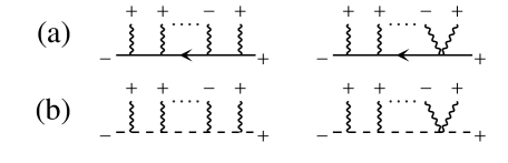
Figure 4: This figure represents contributions to the MHV amplitudes which enjoy a close supersymmetric similarity. The text describes the simple relationship between the (a) second order fermionic and (b) scalar amplitudes.

Now, with reference to Fig. 4, we shall compare the product of terms used in each of the diagrams that contribute to the fermion (Fig. 4a) and the scalar (Fig. 4b) amplitudes. Such amplitudes are termed maximally helicity violating (MHV), because they are those amplitudes with the most external legs of the same helicity that are not identically zero at tree level.

In terms of the second order rules, we can see quite quickly that the ${\cal A}^{\psi}(++;\ldots+)$ and ${\cal A}^{\psi}(-+;\ldots+)$ amplitudes vanish. The former because each of the rules is helicity conserving and $\left\langle n^{+}|\ p_{\psi}^{+}\right\rangle=0$ (this result is also obvious when using the first order rules). The latter follows from the following fact,

$$\left\langle n^{-}\right|[{\raise-0.34723pt\hbox to4.05904pt{\hss/\hss}\hbox to0.0pt{\hss$\epsilon$}}^{+}(p;r),{\raise-1.31944pt\hbox to5.03125pt{\hss/\hss}\hbox to0.0pt{\hss$p$}}]=0$$ (30)

(see Eq. (28))—that is to say, where all the photon helicities are opposite to that of the leading spinor the fermion and scalar vertices are effectively identical. Choosing the arbitrary spinor momentum at the head of the fermion line to be equal to the momentum of the trailing spinor, $x=p_{\psi}$, gives an amplitude proportional to $\left\langle p_{\psi}^{-}|\ p_{\psi}^{+}\right\rangle/\left\langle p_{\psi}^{+}|\ p_{\bar{\psi}}^{-}\right\rangle=0$. In this latter case the proportionality factor is the scalar amplitude, ${\cal A}^{\phi}(-+;\ldots+)$. This can be seen to be zero by choosing the reference momenta of every polarization vector to be equal to momentum of the trailing spinor, $p_{\psi}$. So in fact both of these fermion amplitudes are zero independent of our choice for $x$. This can also be seen as a consequence of supersymmetric Ward identities [14].

For the MHV amplitudes the relationship between the scalar and fermionic amplitudes is almost as simple as that of the ${\cal A}(-+;\ldots+)$ case. This is because each of the three-point vertices that couple the positive helicity photons to the fermion are effectively just scalar vertices (see Eq. (30)). The difference between the fermion and scalar amplitudes is due solely to the uniquely fermionic component of the negative helicity three-point vertex. This contribution is of the form (see the first of the graphs Fig. 4a and Eq. (28)),

$$\frac{\sqrt{2}igQ}{\left\langle x^{-}|\ p_{\bar{\psi}}^{+}\right\rangle}\left\langle x^{-}\right|\;S_{\rm before}\;\left|p_{(-)}^{+}\right\rangle\left\langle p_{(-)}^{-}\right|\;S_{\rm after}\;\left|p_{\psi}^{+}\right\rangle$$ (31)

where $p_{(-)}$ is the momentum of the negative helicity photon. $S_{\rm before(after)}$ is the product of the preceding(trailing) scalar-like vertices and propagators, which freely commute with $\left\langle x^{-}\right|$. Clearly the choice, $x=p_{(-)}$, removes this contribution from the amplitude.

Using Eq. (27) with the choice $n=p_{(-)}$ for the spinor reference momentum, it becomes trivial with the second order rules to demonstrate in a perturbative sense that each of the diagrams contributing to these tree level MHV amplitudes (and accordingly the amplitudes themselves) are related by,

$${\cal A}^{\psi}(-+;\ldots-\ldots+)=\frac{\left\langle p_{(-)}^{-}|\ p_{\psi}^{+}\right\rangle}{\left\langle p_{(-)}^{-}|\ p_{\bar{\psi}}^{+}\right\rangle}{\cal A}^{\phi}(-+;\ldots-\ldots+).$$ (32)

It is amusing to note that this diagram-by-diagram equivalence is even independent of the choice of reference momenta for the photon polarization vectors. At the level of the amplitude this is of course in complete agreement with the appropriate supersymmetric Ward identity [14].

In this letter, we have discussed the second order formalism for fermions and have succeeded in rewriting the Feynman rules for gauged-fermions in a form that exposes their close similarity to gauged-scalars. We have shown how these rules may be applied to the calculation of both closed fermion loops and for processes involving external fermions. Because of the close relationship between the second order rules and the first quantized form [4, 5], this work may provide some reference for those wishing to construct string-like rules for external fermions.

The supersymmetric relationship between fermion and scalar loops has been investigated previously [1, 2, 6] where the second order formalism, as it applied to closed fermion loops, was employed. Here, we have demonstrated that this similarity exists for external fermions too. We have used it in a simple example, to make transparent the supersymmetric Ward identity relating two MHV amplitudes, which is something not normally obvious at the level of individual Feynman diagrams.

Although the simple relationship presented in the above example is more complicated for other helicity configurations, it will always be the case that a fermion amplitude has a component which is directly proportional to a scalar one—a feature which is explicit with the second order Feynman rules. This component is physical, insofar as it is gauge invariant. So by choosing a different set of reference momenta for the external gauge bosons, we may optimize the calculation of the fermionic remainder. That is to say, such a remainder may be calculated more efficiently on its own than when mixed up with the rest of the amplitude. This method of breaking-up amplitudes has already been used successfully for closed fermion loops [6], and can be thought of as a generalization of the established supersymmetric techniques [15, 13].

References

- [1] Z. Bern and D.A. Kosower, Nucl. Phys. B379 (1992) 451.
- [2] Z. Bern and D.C. Dunbar, Nucl. Phys. B379 (1992) 562.
- [3] C.S. Lam, Phys. Rev. D48 (1993) 873; (hep-ph/9308289) Can. J. Phys. Vol. 72 (1994) 415.
- [4] L. Brink, P. Di Vecchia and P. Howe, Phys. Lett. 65B (1976) 471; Nucl. Phys. B118 (1977) 76; E.S. Fradkin, A.A. Tseytlin; Phys. Lett. 158B (1985) 316; Phys. Lett. 163B (1985) 123; Nucl. Phys. B261 (1985) 1; A.M. Polyakov, “Gauge Fields and Strings”, Harwood (1987); M.G. Schmidt and C. Schubert, (hep-ph/9408394) HD-THEP-94-32; (hep-th/9410100) HD-THEP-94-25; (hep-ph/9412358) HD-THEP-94-33; D. Cangemi, E. D’Hoker and G. Dunne, (hep-th/9409113) UCLA-94-TEP-35 (1994).
- [5] M.J. Strassler, (hep-ph/9205205) Nucl. Phys. B385 (1992) 145.
- [6] Z. Bern, L. Dixon and D.A. Kosower, (hep-ph/9302280) Phys. Rev. Lett. 70 (1993) 2677; (hep-ph/9306240) Nucl. Phys. B412 (1994) 751; D.C. Dunbar and P.S. Norridge, (hep-th/9408014) UCLA-TEP-94-30; Z. Bern and A.G. Morgan, (hep-ph/9312218) Phys. Rev. D49 (1994) 6155.
- [7] L.D. Faddeev and V.N. Popov, Phys. Lett. B25 (1967) 29.
-
[8]
See for example,
C. Itzykson and I. Zuber, “Quantum Field Theory”, McGraw-Hill Inc., (1980); L.H. Ryder, “QUANTUM FIELD THEORY”, Wiley (1984). - [9] J.E. Paton and H.M. Chan, Nucl. Phys. B10 (1969) 516; F.A. Berends and W.T. Giele, Nucl. Phys. B294 (1987) 700; M. Mangano and S.J. Parke, Nucl. Phys. B299 (1988) 673; M. Mangano, Nucl. Phys. B309 (1988) 461; Z. Bern and D.A. Kosower, Nucl. Phys. B362 (1991) 389.
- [10] F. A. Berends, R. Kleiss, P. De Causmaecker, R. Gastmans and T. T. Wu, Phys. Lett. B103 (1981) 124; P. De Causmaeker, R. Gastmans, W. Troost and T. T. Wu, Nucl. Phys. B206 (1982) 53; J. F. Gunion and Z. Kunszt, Phys. Lett. B161 (1985) 333; R. Gastmans and T.T. Wu, “The Ubiquitous Photon: Helicity Method for QED and QCD”, Clarendon Press (1990) .
- [11] R. Kleiss and W. J. Stirling, Nucl. Phys. B262 (1985) 235.
- [12] Z. Xu, D.-H. Zhang and L. Chang, Nucl. Phys. B291 (1987) 392.
- [13] M.L. Mangano and S.J. Parke, Phys. Reports 200:6 (1991) 301.
- [14] M.T. Grisaru and H.N. Pendleton, Nucl. Phys. B124 (1977) 81; M.T. Grisaru, H.N. Pendleton and P. van Nieuwenhuizen, Phys. Rev. D15 (1977) 996; S.J. Parke and T.R. Taylor, Phys. Lett. B157 (1985) 81.
- [15] Z. Kunszt, Nucl. Phys. B271 (1986) 333.