A Precision Calculation of the Next-to-Leading Order Energy-Energy Correlation Function

Abstract

The $O(\mbox{$\alpha_{s}$}^{2})$ contribution to the Energy-Energy Correlation function (EEC) [1, 2, 3, 4] of $\mbox{e${}^{+}$ e${}^{-}$}\rightarrow$ hadrons is calculated to high precision and the results are shown to be larger than previously reported [9, 10, 11, 12, 13]. The consistency with the leading logarithm approximation and the accurate cancellation of infrared singularities exhibited by the new calculation suggest that it is reliable. We offer evidence that the source of the disagreement with previous results lies in the regulation of double singularities.

UW/PT 94-17 hep-ph/9502223

A Precision Calculation of the Next-to-Leading Order Energy-Energy Correlation Function

Keith A. Clay and Stephen D. Ellis Department of Physics, University of Washington

January 30, 1995

The energy-energy correlation function (EEC) [1, 2, 3, 4] for e⁺ e^-annihilation into hadrons is widely used as a measure of the strong coupling constant $\alpha_{s}$ [5, 6, 7] and is potentially one of the most precise and detailed experimental tests of QCD available [7, 8]. However, that potential has not been realized due to disagreement over the predicted value of the next-to-leading order correction in the strong coupling constant [9, 10, 11, 12, 13]. We report on a new calculation of the $O(\mbox{$\alpha_{s}$}^{2})$ term using subtraction for control of infrared singularities. Accuracy was checked at every stage by symbolic computation, high precision arithmetic, and human calculation. The detailed cancellation of singularities in the complicated four-parton states was carefully tested. A more complete description will be presented elsewhere [14].

The EEC was invented to take advantage of the asymptotic freedom of QCD by viewing the products of e⁺ e^-annihilation with a weighting that favored the most energetic hadrons [1, 3, 4]. Conservation of energy requires all energy carried by quarks and gluons to be transferred to detectable hadrons, hence the EEC is experimentally and theoretically defined as

$$\frac{d\Sigma}{d\cos(\chi)} \equiv \lim_{\stackrel{{\scriptstyle N\rightarrow\infty}}{{\scriptstyle{\Delta\rightarrow 0}}}}\;\sum_{N\;events}\left(\left(\frac{\sigma}{N\,\Delta}\right)\sum_{\stackrel{{\scriptstyle\scriptstyle{hadrons\;a,b}}}{{\scriptstyle{\left|{\bf\hat{p}}_{a}\cdot{\bf\hat{p}}_{b}-\cos(\chi)\right|<\Delta}}}}\left(\frac{E_{a}\,E_{b}}{E_{total}^{2}}\right)\right)$$ (1)

$$= \sum_{partons\;i,j}\,\int d^{3}{\bf\vec{p}}_{i}\;d^{3}{\bf\vec{p}}_{j}\left(\frac{d\sigma}{d^{3}{\bf\vec{p}}_{i}\,d^{3}{\bf\vec{p}}_{j}}\right)\left(\frac{E_{i}\,E_{j}}{E_{total}^{2}}\right)\delta\!\left({\bf\hat{p}}_{i}\!\cdot\!{\bf\hat{p}}_{j}-\cos(\chi)\right)$$

where $\sigma$ is the total cross section for $\mbox{e${}^{+}$ e${}^{-}$}\rightarrow$ hadrons, $E_{n}$ and ${\bf\vec{p}}_{n}$ are the energy and momentum of particle $n$, and $E_{total}$ is the center of mass energy of the system. The EEC is free of collinear singularities since all parallel momenta are linearly summed [15].

After factoring out the trivial dependence on the total cross section and $\sin^{2}\chi$ [12], the EEC has the following perturbative expansion in the region $0<\chi<\pi$,

$$\frac{d\Sigma}{d\cos(\chi)}\equiv \left(\frac{\mbox{$\sigma_{0}$}}{\mbox{$\sin^{2}\chi$}}\right)\left\{\left(\frac{\mbox{$\alpha_{s}$}}{2\pi}\right)\mbox{${\cal A}(\chi)$}\,\left[1+\left(\frac{\mbox{$\alpha_{s}$}}{2\pi}\right)\,\beta_{0}\,\log\left(\frac{\mu}{E_{total}}\right)\right]+\left(\frac{\mbox{$\alpha_{s}$}}{2\pi}\right)^{2}\mbox{${\cal B}(\chi)$}+O\!\left(\mbox{$\alpha_{s}$}^{3}\right)\right\}\,.$$ (2)

Here $\sigma_{0}$ is the leading order total cross section, $\mu$ is the renormalization scale, and $\beta_{0}$ is the leading coefficient of the $\beta$ function: $\beta_{0}=\frac{11}{3}C_{A}-\frac{4}{3}T_{R}$. For QCD in this notation, $C_{F}=\frac{4}{3}$, $C_{A}=3$, and $T_{R}=\frac{1}{2}N_{F}$, where $N_{F}$ is the number of active quark flavors at energy $E_{total}$. Analytic calculation of ${\cal A}$ yields [1]

$${\cal A}(\chi) = \;C_{F}\;(1+\omega)\,(1+3\omega)\left[(2-6\omega^{2})\log\left(1+\omega^{-1}\right)+6\omega-3\right]$$ (3)

where $\omega=\cot^{2}\left(\chi/2\right)$. No such analytic expression is possible for ${\cal B}(\chi)$. At $O(\mbox{$\alpha_{s}$}^{2})$, the EEC receives contributions from four-parton final states at tree level and from three-parton final states with a virtual parton forming one internal loop. The three-parton final states pose little challenge, but the integrals corresponding to four-parton states with an external angle fixed at $\chi$ demand numerical as well as analytic calculation.

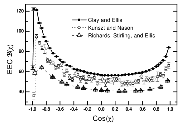
Figure 1: The $O(\mbox{$\alpha_{s}$}^{2})$ contribution to the Energy-Energy Correlation function. For comparison we display our results (solid circles), the results of Kunszt and Nason [12] (open squares), and the results of Richards, Stirling, and Ellis [10] (open triangles). ${\cal B}$ values shown are for five active quark flavors or $T_{R}=\frac{5}{2}$ (see equation 5).

To calculate contributions near soft or collinear poles, the four-parton expressions were simplified to allow analytic integration in the presence of an infrared regulator $\epsilon$ (dimension $D=4-2\epsilon$). Using the subtraction method of infrared regulation, the simplified expressions were subtracted from exact expressions and the finite difference was numerically integrated without infrared regulation ($\epsilon=0$). Analytic integrals of the three-parton and simplified four-parton expressions (at finite $\epsilon$) were then added and the sum was shown to remain finite in the limit $\epsilon\rightarrow 0$. As in all previous calculations of ${\cal B}$, we used the expressions derived by Ellis, Ross, and Terrano (ERT) [16] for the exact three-parton and four-parton final states, but we did not use the ERT simplifications or analytic integrals for reasons of maximizing numerical convergence.

Our results (Clay and Ellis or CE) are plotted in Figure 1 along with the results previously reported by Richards, Stirling, and Ellis (RSE) [10] and Kunszt and Nason (KN) [12]. The mean relative numerical uncertainty in our calculation is 0.3%, while for KN it is roughly 4%, both arising from the precision of numerical integrations. This uncertainty is insufficient to explain the roughly 15% overall difference between KN and CE. While it is possible for systematic differences such as these to arise from purely numerical errors, we believe there is an analytic error at the heart of the disagreement.

Coefficient	Exact	Clay and Ellis	Richards, Stirling
	Value		and Ellis
${\cal B}^{+}_{3}$	$-2\;C_{F}$	$(-2.017\pm 0.049)\;C_{F}$	$(-2.46\pm 0.29)\;C_{F}$
${\cal B}^{+}_{2}$	$9\;C_{F}\;+$	$(9.84\pm 0.90)\;C_{F}\;+$	$(21.0\pm 9.0)\;C_{F}\;+$
	$3.67\;C_{A}\;+$	$(3.63\pm 0.12)\;C_{A}\;+$	$(2.86\pm 7.24)\;C_{A}\;+$
	$-1.333\;T_{R}$	$(-1.333\pm 0.001)\;T_{R}$	$(-1.35\pm 0.05)\;T_{R}$
${\cal B}^{+}_{1}$	$-23.6\;C_{F}\;+$	$(-20.6\pm 4.79)\;C_{F}\;+$	$(-140\pm 111)\;C_{F}\;+$
	$-1.34\;C_{A}\;+$	$(-1.53\pm 2.11)\;C_{A}\;+$	$(14.0\pm 71.7)\;C_{A}\;+$
	$-0.222\;T_{R}$	$(-0.220\pm 0.03)\;T_{R}$	$(-0.066\pm 0.480)\;T_{R}$
${\cal B}^{+}_{0}$	$26.2\;C_{F}\;+$	$(23.1\pm 5.89)\;C_{F}\;+$	$(370\pm 196)\;C_{F}\;+$
	$16.6\;C_{A}\;+$	$(13.43\pm 9.00)\;C_{A}\;+$	$(-56.8\pm 228)\;C_{A}\;+$
	$-3.58\;T_{R}$	$(-3.58\pm 0.17)\;T_{R}$	$(-4.16\pm 1.64)\;T_{R}$
${\cal B}^{-}_{1}$	$-3.125\;C_{F}\;+$	$(-3.15\pm 0.04)\;C_{F}\;+$	$(6.51\pm 0.35)$
	$3.567\;C_{A}\;+$	$(3.57\pm 0.01)\;C_{A}\;+$	(exact $=6.533$) $\;+$
	$-0.8833\;T_{R}$	$(-0.8832\pm 0.0005)\;T_{R}$	$(-0.88\pm 0.02)\;T_{R}$
${\cal B}^{-}_{0}$	?	$(8.69\pm 0.40)\;C_{F}\;+$	$29.9\pm 2.9$
	?	$(15.7\pm 0.2)\;C_{A}\;+$	$(N_{F}\equiv 4)$
	?	$(-5.46\pm 0.005)\;T_{R}$

Table 1: The coefficients of the leading log expansion of the EEC at large (${\cal B}^{+}_{j}$) and small (${\cal B}^{-}_{j}$) angles. The expansion is as shown in equation 4. Listed are the exact leading log coefficients and the coefficients producing the best fit to Clay and Ellis as well as Richards, Stirling, and Ellis [17].

The only known test of the analytic behavior of ${\cal B}$ is a comparison with the predictions of the leading logarithm approximation for large and small angles [2]. To determine asymptotic behavior, ${\cal B}(\chi)$ was calculated over the range $\left|\cos(\chi)\right|\leq(1-10^{-6})$, and the results were compared to an expansion of the form

$$\lim_{\eta^{\pm}\rightarrow 0}\mbox{${\cal B}(\chi)$}=C_{F}\sum_{j=0}^{3}\mbox{${\cal B}^{\pm}_{j}$}\;\left[\ln\!\left(1/\eta^{\pm}\right)\right]^{j}$$ (4)

where $\eta^{\pm}=\frac{1}{2}(1\pm\cos(\chi))$. The coefficients ${\cal B}^{\pm}_{j}$ that best fit our calculation were found using an unconstrained least squares fit and are displayed in Table 1 (we find that ${\cal B}^{-}_{3}={\cal B}^{-}_{2}=0$, as expected). For comparison, we also show the coefficients derived by RSE [17] who reported some inconsistency with the leading logarithm approximation. No inconsistency is evident in our data. The previously unpublished exact values for ${\cal B}^{+}_{0}$ are based on our conjecture that the form factor for the EEC is the same as that for the second energy moment of the Drell-Yan cross section [18, 19]. The form factor is convoluted with a known parton evolution function [20] to produce ${\cal B}^{+}_{0}$.

The discrepancy over the value of ${\cal B}^{-}_{0}$ is significant. With $N_{F}\equiv 4$, RSE extracted a value of ${\cal B}^{-}_{0}$ equal to $29.9\pm 2.9$, while our calculation predicts a value of $47.8\pm 0.8$ (see Table 1). Based on our preliminary analysis of data from KN as well as Glover and Sutton (GS) [13], we conclude that neither is consistent with the values of ${\cal B}^{-}_{0}$ from either CE or RSE. It is unfortunate that the coefficient that best discriminates between the various calculations is unknown. An independent calculation of ${\cal B}^{-}_{0}$ would be very useful for resolving the disagreement.

To explore the source of the disagreement, we parameterize ${\cal B}$ as a sum of three functions

$${\cal B}(\chi) = C_{F}\;\left(\;C_{F}\;\mbox{${\cal B}_{C_{F}}\!(\chi)$}+C_{A}\;\mbox{${\cal B}_{C_{A}}\!(\chi)$}+T_{R}\;\mbox{${\cal B}_{T_{R}}\!(\chi)$}\;\right)$$ (5)

and compare our results for each function with those of GS as well as RSE. While CE and GS [21] differ significantly over ${\cal B}_{C_{A}}$  and even more so over ${\cal B}_{C_{F}}$, they agree with each other and with RSE [10] on the value of ${\cal B}_{T_{R}}$. It was also only for ${\cal B}_{C_{A}}$ and ${\cal B}_{C_{F}}$ that RSE reported difficulty in the fit to leading logarithms [17]. This strongly suggests that the source of the disagreement lies outside of the calculation of ${\cal B}_{T_{R}}$and is most severely manifest in that of ${\cal B}_{C_{F}}$.

We believe that the source of disagreement is the regulation of double (i.e., soft and collinear) infrared singularities. Calculation of ${\cal B}_{T_{R}}$ involves no such regulation since the four-fermion states have no soft singularities, while unique to ${\cal B}_{C_{F}}$ are “ladder diagram” contributions that produce the double singularities least controlled by energy weighting.

To deal with infrared singularities, the exact perturbative integrands are simplified in such a way as to be analytically integrable in the presence of an infrared regulator (e.g., $4-2\epsilon$ dimensions) while producing integrated expressions that display the same singular dependence on the regulator (e.g., poles in $\epsilon$) as do integrals of the exact integrands. The simplified integrands are also used in numerical integrations where the regulator is necessarily removed ($\epsilon\rightarrow 0$) before integration. Any such algorithm guarantees that the singular parts of the dependence on the regulator will be correctly calculated.

We have found that simplifications of integrands involving double poles can produce non-singular ($O(\epsilon^{0})$) errors from inexact treatment of $O(1/\epsilon)$ shoulders of the $O(1/\epsilon^{2})$ double poles multiplying terms of $O(\epsilon)$. Since energy weighting can reposition these shoulders in a complicated way, simplified EEC integrands may be especially prone to such errors. These errors cannot be corrected in any numerical integrals where $\epsilon\rightarrow 0$ prior to integration. The subtraction method prescribes addition and subtraction of the same quantity but the added quantities are integrated analytically while subtracted quantities must be integrated numerically to cancel poles in the exact four-parton integrands. Thus the added and subtracted quantities may differ due to necessarily different regulation methods for the numerical and analytic integrals. In such cases, integration of the difference between simplified and exact integrands is not uniformly convergent near double poles and the integrals are finite only in the sense of a numerically computed average. This average will generally not be the correct result obtained by analytically setting $\epsilon\rightarrow 0$ after completing integration rather than before.

As a test for these errors in our calculation, the cancellation of double singularities was examined. Since analytic work is difficult for the four-parton states, we have focused on tests of numerical convergence. The scale of the independent variable controlling the singularities was magnified by a factor of $10^{4}$ in a search for instabilities and neighborhoods of double poles were divided into separately integrated patches to isolate divergences. While further study is required, neither test produced signs of non-uniform convergence or error.

Ultimately theory must be compared with experiment, and fits of our calculation to data from SLD [7] have been performed [22]. Using the procedure adopted in [7], values for $\alpha_{s}(M_{Z})$ were derived using the EEC as well as the asymmetry of the EEC or AEEC:

$$\mbox{$AEEC(\chi)\equiv EEC(\pi-\chi)-EEC(\chi)$}.$$

Renormalization scales used were in the range

$$\left.\begin{array}[]{c}{\ 0.0035\;{\textstyle(EEC)}}\\ {\ 0.09\;{\textstyle(AEEC)}}\end{array}\right\}\leq\left(\frac{\mu^{2}}{E_{total}^{2}}\right)\leq 4,$$

and while fits using KN and CE were found to have similar $\mu$ dependence, EEC fits using the larger CE values for ${\cal B}$ yield $\alpha_{s}(M_{Z})$ values smaller by about 0.005 [22, 23]. Although all ${\cal B}$ calculations yield larger $\alpha_{s}(M_{Z})$ values from EEC fits than from AEEC fits [7], it is interesting to note that the two differ by 0.012 for KN, as opposed to only 0.006 for CE [7, 22, 23]:

$$\mbox{$\alpha_{s}$}^{(EEC)}_{(CE)}(M_{Z}) = 0.118\pm 0.013{\em(scale)}\pm 0.002{\em(hadronization)}\pm 0.003{\em(experiment)},$$

$$\nopagebreak\mbox{$\alpha_{s}$}^{(AEEC)}_{(CE)}(M_{Z}) = 0.112\pm 0.003{\em(scale)}\pm 0.002{\em(hadronization)}\pm 0.003{\em(experiment)}.$$ (6)

While the improved agreement does not constitute evidence that our calculation is correct, it is an attractive and suggestive feature of the results.

We conclude that the disagreement over the next-to-leading order contribution to the EEC has not been resolved. Comparison of our calculation with all that is known about the EEC shows it to be reasonable and numerically reliable despite disagreement with previous calculations. A more intensive investigation of the cancellation of double singularities combined with a possible extension of our knowledge of the leading logarithm expansion is needed to resolve the differences.

Acknowledgments:

The authors gratefully acknowledge many helpful discussions with P. Burrows and H. Masuda concerning experimental results from SLD, and many useful communications with E.W.N. Glover concerning his results. This research was supported by the U.S. Department of Energy, grant number DE-FG06-91ER40614.

References

- [1] C. L. Basham, L. S. Brown, S. D. Ellis, and S. T. Love, Phys. Rev. D17 (1978) 2298; ibid. D19 (1979) 2018; ibid. D24 (1981) 2382; Phys. Rev. Lett. 41 (1978) 1585.
- [2] C. L. Basham, L. S. Brown, S. D. Ellis, and S. T. Love, Phys. Lett. 85B (1979) 297.
- [3] L. S. Brown and S. D. Ellis, Phys. Rev. D24 (1981) 2383.
- [4] L. S. Brown, in High Energy Physics in the Einstein Centennial Year, ed. B. Kursunoglu, Plenum Publishing, (1979) p. 373
- [5] DELPHI Collaboration, P. Abreu et al., Phys. Lett. 252B (1990) 149.
- [6] OPAL Collaboration, M. Akrawy et al., Phys. Lett. 252B (1990) 159; ibid. 296B (1992) 547.
- [7] SLD Collaboration, K. Abe et al., SLAC-PUB-6641 (1994) to appear in Phys. Rev. D51 (1995); Phys. Rev. D50 (1994) 5580.
- [8] S. Bethke, in the Proceedings of the XXVI International Conference on High Energy Physics, ed. J. Sanford, (1992) p. 81
- [9] A. Ali and F. Barreiro, Phys. Lett. 118B (1982) 155; Nucl. Phys. B236 (1984) 269.
- [10] D. G. Richards, W. J. Stirling, and S. D. Ellis, Phys. Lett. 119B (1982) 193; Nucl. Phys. B229 (1983) 317.
- [11] N. K. Falck and G. Kramer, Z. Phys, C42 (1989) 459.
- [12] Z. Kunszt and P. Nason, Z physics at LEP 1, CERN 89-08, vol 1, (1989) p. 373
- [13] E. W. N. Glover and M. R. Sutton, University of Durham preprint DTP/94/80, (1994).
- [14] K. A. Clay and S. D. Ellis, in preparation.
- [15] G. Sterman and S. Weinberg, Phys. Rev. Lett. 39 (1977) 1436.
- [16] R. K. Ellis, D. A. Ross, and A. E. Terrano, Nucl. Phys. B178 (1981) 421.
- [17] D. G. Richards, W. J. Stirling, and S. D. Ellis, Phys. Lett. 136B (1984) 99.
- [18] C. T. H. Davies and W. J. Stirling, Nucl. Phys. B244 (1984) 337.
- [19] C. T. H. Davies, B. R. Webber, and W. J. Stirling, Nucl. Phys. B256 (1985) 413.
- [20] J. C. Collins, D. E. Soper, Nucl. Phys. B193 (1981) 381; ibid. B197 (1982) 446; ibid. B284 (1987) 253.
- [21] E. W. N. Glover and M. R. Sutton, personal communication.
- [22] P. Burrows and H. Masuda, personal communication.
- [23] SLD Collaboration, K. Abe et al., SLAC-PUB-95-6739 (1995), submitted to Phys. Rev. D. (rapid communications).