SHEP 94-05

Fermion Masses in a Supersymmetric SU(4)$\otimes$SU(2)${}_{L}\otimes$SU(2)_R Model

B. C. Allanach and S. F. King

Physics Department, University of Southampton
Southampton, SO17 5NH, U.K.

Abstract

We calculate quark and lepton masses and quark mixing angles in the framework of a supersymmetric SU(4)$\otimes$SU(2)${}_{L}\otimes$SU(2)_R model where the gauge group is broken at 10¹⁶ GeV. The model predicts third family top-bottom-tau Yukawa unification, as in minimal SO(10). The other smaller Yukawa couplings are assumed to arise from non-renormalisable operators suppressed by powers of some heavy scale. We perform a systematic operator analysis of the model in order to find the minimum set of operators which describe the low energy quark and lepton masses, and quark mixing angles consistent with low-energy phenomenology. A novel feature of the model is the possibility of asymmetric texture zeroes in the Yukawa matrices at the scale of the new physics. Successful predictions are obtained for $m_{t}$, $\tan\beta$, $m_{s}/m_{\mu}$, $m_{d}/m_{e}$ and $V_{ub}$ in terms of a CP violating phase $\phi$. For example, we predict $\tan\beta=35-65$, $m_{t}=130-190$ GeV, and $|V_{ub}|>0.0040$.

1 Introduction

The problem of quark and lepton masses is one of the most fascinating and perplexing problems of particle physics. The standard model, despite its successes, can offer no glimpse of insight into the apparently bizarre pattern of masses and mixing angles which experiment has presented us with. We do not even know why there are three families rather than one. It is clear, then, that in order to gain some insight into the fermion mass problem, one must go beyond the standard model. The big question of course is what lies beyond it?

We have not yet experimentally studied the mechanism of electroweak symmetry breaking, so one might argue that it is premature to study the fermion mass problem. Unless we can answer this, we have no hope of understanding anything about fermion masses since we do not have a starting point from which to analyse the problem. However LEP has taught us that whatever breaks electroweak symmetry must do so in a way which very closely resembles the standard model. This observation by itself is enough to disfavour many dynamical models involving large numbers of new fermions. By contrast the minimal supersymmetric standard model (MSSM) mimics the standard model very closely. Furthermore, by accurately measuring the strong coupling constant, LEP has shown that the gauge couplings of the MSSM merge very accurately at a scale just above $10^{16}$ GeV, thus providing a hint for possible unification at this scale. On the theoretical side, supersymmetry (SUSY) and grand unified theories (GUTs) fit together very nicely in several ways, providing a solution to the technical hierarchy problem for example. When SUSY GUTs are extended to supergravity (SUGRA) the beautiful picture of universal soft SUSY breaking parameters and radiative electroweak symmetry breaking via a large top quark yukawa coupling emerges. Finally, there is an on-going effort to embed all of this structure in superstring models, thereby allowing a complete unification, including gravity.

Given the promising scenario mentioned above, it is hardly surprising that many authors have turned to the SUSY GUT framework as a springboard from which to attack the problem of fermion masses [1]. Indeed in recent years there has been a flood of papers on fermion masses in SUSY GUTs. Although the approaches differ in detail, there are some common successful themes which have been known for some time. For example the idea of bottom-tau Yukawa unification in SUSY GUTs [2] works well with current data [3]. A more ambitious extension of this idea is the Georgi-Jarlskog (GJ) ansatz which provides a successful description of all down-type quark and charged lepton masses [4, 16], and which also works well with current data [5]. The GJ approach involves the idea of texture zeroes and predicts simple relations at the unification scale which are then evolved to low-energies using the renormalisation group (RG) equations. These approaches are concerned with general properties of the mass matrices, rather than those of specific models.

In order to understand the origin of the texture zeroes, one must consider the details of the model above the scale $M_{X}\sim 10^{16}$ GeV (SO(10) for example in the case of GJ). While one might not wish to restrict oneself to some particular gauge symmetry at $M_{X}$, it is almost essential to specify the model at this scale in order to make any progress at all. The alternative is to simply make a list of assumptions about the nature of the Yukawa matrices at $M_{X}$ [6]. For example Ramond, Roberts and Ross (RRR) [7] assumed symmetric Yukawa matrices at $M_{X}$, together with the GJ ansatz for the lepton sector. It is difficult to proceed beyond this without specifying a particular model. Indeed, this model dependence may be a good thing since it may mean that the fermion mass spectrum at low energies is sensitive to the theory at $M_{X}$, so it can be used as a window into the high-energy theory. Therefore in what follows we shall restrict ourselves to the very specific gauge group at $M_{X}$ referred to in the title. Our motivation for considering this particular theory is discussed below.

Twenty-one years ago Pati and Salam proposed a model in which the standard model was embedded in the gauge group SU(4)$\otimes$SU(2)${}_{L}\otimes$SU(2)_R [8]. More recently a superpersymmetric (SUSY) version of this model was proposed in which the gauge group is broken at $M_{X}\sim 10^{16}$ GeV [9]. The model [9] does not involve adjoint representations and later some attempt was made to derive it from four-dimensional strings, although there are some difficulties with the current formulation [10]. In this paper we shall not be concerned with the superstring formulation of the model, but instead we shall focus on the “low-energy” effective field theory. The absence of adjoint representations is not an essential prerequisite for the model to descend from the superstring, but it leads to some technical simplifications. Also in the present model, the colour triplets which are in separate representations from the Higgs doublets, become heavy in a very simple way so the Higgs doublet-triplet splitting problem does not arise. These two features (absence of adjoint representations and absence of the doublet-triplet splitting problem,) are shared by flipped SU(5)$\otimes$U(1) [11], which also has a superstring formulation. Although the present model and flipped SU(5)$\otimes$U(1) are similar in many ways, there are some important differences. Whereas the Yukawa matrices of flipped SU(5)$\otimes$U(1) are completely unrelated at the level of the effective field theory at $M_{X}$ (although they may have relations coming from the string model) in the present model there is a constraint that the top, bottom and tau Yukawa couplings must all unify at that scale. In addition there will be Clebsch relations between the other elements of the Yukawa matrices, assuming they are described by non-renormalisable operators, which would not be present in flipped SU(5)$\otimes$U(1). In these respects the model resembles the SO(10) model recently analysed by Anderson et al [12]. However it differs from the SO(10) model in that the present model does not have an SU(5) subgroup which is central to the analysis of the SO(10) model. In addition the operator structure of the present model is totally different. Thus the model under consideration is in some sense similar to flipped SU(5)$\otimes$U(1), but has third family Yukawa unification and precise Clebsch relationships as in SO(10). We find this combination of features quite remarkable, and it seems to us that this provides a rather strong motivation to study the problem of fermion masses in this model.

The problem of fermion masses in the SU(4)$\otimes$SU(2)${}_{L}\otimes$SU(2)_R model was recently considered by one of us [13]. It was implicitly assumed that the Yukawa matrices were symmetric, and it was shown that by introducing suitable operators the model could make contact with the successful RRR ansatz, which incorporate the GJ ansatz, at the expense of fine-tuning the coefficients of the operators [13]. Essentially the small entries in the RRR matrices were obtained by assuming that the coefficients of two operators were tuned to partially cancel. The purpose of the present paper is threefold. First we shall generalise the analysis to the case of non-symmetric Yukawa matrices, since there is no symmetry which enforces symmetric Yukawa matrices in this model. This allows the possibility of asymmetric texture zeroes, which as far as we are aware have never been considered before. Of course this means that we cannot rely on the RRR analysis, and therefore we perform our own phenomenological analysis of the quark and lepton masses and quark mixing angles. Second we extend the operator analysis to consider many other operators not considered in the previous analysis. In fact we search for all possible low dimensional operators, and systematically search for the minimum set with which to describe the spectrum. Third we impose a naturalness criterion and reject all possibilities which involve fine-tuning the coefficients of operators. The result of all this is a small set of possible solutions to the problem of quark and lepton masses and CKM angles in this model.

The remainder of the paper is organised as follows. In section 2 we briefly summarise the model. In section 3 we describe the operator strategy we employ. In section 4 the details of the calculation are outlined, including the RG and CKM analysis. The ansatze, results and predictions are presented. Section 5 contains our conclusions about the previous analysis, and a brief discussion of theoretical uncertainties involved with the calculation. In the appendices we list the operators in explicit component form.

2 The Model

Here we briefly summarise the parts of the model which are relevant for our analysis. For a more complete discussion see [9]. The gauge group is,

$$\mbox{SU(4)}\otimes\mbox{SU(2)}_{L}\otimes\mbox{SU(2)}_{R}.$$ (1)

The left-handed quarks and leptons are accommodated in the following representations,

$${F^{i}}^{\alpha a}=(4,2,1)=\left(\begin{array}[]{cccc}u^{R}&u^{B}&u^{G}&\nu\\ d^{R}&d^{B}&d^{G}&e^{-}\end{array}\right)^{i}$$ (2)

$${\bar{F}}_{x\alpha}^{i}=(\bar{4},1,\bar{2})=\left(\begin{array}[]{cccc}\bar{d}^{R}&\bar{d}^{B}&\bar{d}^{G}&e^{+}\\ \bar{u}^{R}&\bar{u}^{B}&\bar{u}^{G}&\bar{\nu}\end{array}\right)^{i}$$ (3)

where $\alpha=1\ldots 4$ is an SU(4) index, $a,x=1,2$ are SU(2)_L,R indices, and $i=1\ldots 3$ is a family index. The Higgs fields are contained in the following representations,

$$h_{a}^{x}=(1,\bar{2},2)=\left(\begin{array}[]{cc}{h_{2}}^{+}&{h_{1}}^{0}\\ {h_{2}}^{0}&{h_{1}}^{-}\\ \end{array}\right)$$ (4)

(where $h_{1}$ and $h_{2}$ are the low energy Higgs superfields associated with the MSSM.) The two heavy Higgs representations are

$${H}^{\alpha b}=(4,1,2)=\left(\begin{array}[]{cccc}u_{H}^{R}&u_{H}^{B}&u_{H}^{G}&\nu_{H}\\ d_{H}^{R}&d_{H}^{B}&d_{H}^{G}&e_{H}^{-}\end{array}\right)$$ (5)

and

$${\bar{H}}_{\alpha x}=(\bar{4},1,\bar{2})=\left(\begin{array}[]{cccc}\bar{d}_{H}^{R}&\bar{d}_{H}^{B}&\bar{d}_{H}^{G}&e_{H}^{+}\\ \bar{u}_{H}^{R}&\bar{u}_{H}^{B}&\bar{u}_{H}^{G}&\bar{\nu}_{H}\end{array}\right).$$ (6)

The Higgs fields are assumed to develop VEVs,

$$<H>=<\nu_{H}>\sim M_{X},\ \ <\bar{H}>=<\bar{\nu}_{H}>\sim M_{X}$$ (7)

leading to the symmetry breaking at $M_{X}$

$$\mbox{SU(4)}\otimes\mbox{SU(2)}_{L}\otimes\mbox{SU(2)}_{R}\longrightarrow\mbox{SU(3)}_{C}\otimes\mbox{SU(2)}_{L}\otimes\mbox{U(1)}_{Y}$$ (8)

in the usual notation. Under the symmetry breaking in Eq.8, the Higgs field $h$ in Eq.4 splits into two Higgs doublets $h_{1}$, $h_{2}$ whose neutral components subsequently develop weak scale VEVs,

$$<h_{1}^{0}>=v_{1},\ \ <h_{2}^{0}>=v_{2}$$ (9)

with $\tan\beta\equiv v_{2}/v_{1}$.

In addition to the Higgs fields in Eqs. 5,6 the model also involves an SU(4) sextet field $D=(6,1,1)$ and three singlet fields $\phi_{m}=(1,1,1)$ which do not acquire VEVs plus one singlet field $N=(1,1,1)$ which acquires a weak scale VEV $<N>=x$. The superpotential, suppressing gauge indices, is then [9]

$$W=\lambda^{ij}_{1}F_{i}\bar{F}_{j}h+\lambda^{im}_{2}\bar{F}_{i}H\phi_{m}+\lambda_{3}HHD+\lambda_{4}\bar{H}\bar{H}D+\lambda_{5}hhN+\lambda_{6}^{mnq}\phi_{m}\phi_{n}\phi_{q}+\lambda_{7}N^{3}$$ (10)

Note that this is not the most general superpotential invariant under the gauge symmetry. Additional terms not included in Eq.10 may be forbidden by imposing suitable discrete symmetries, the details of which need not concern us here. The $D$ field does not develop a VEV but the terms in Eq.10 $HHD$ and $\bar{H}\bar{H}D$ combine the colour triplet parts of $H$, $\bar{H}$ and $D$ into acceptable GUT-scale mass terms [9]. The $\phi_{m}$ fields play an important part in ensuring that the right-handed neutrinos gain large masses, leading to acceptably small observable neutrino masses. The effect depends on terms in the superpotential like $\bar{F}H\phi$ and $\phi^{3}$ [14]. Below $M_{X}$ the part of the superpotential involving quark and charged lepton fields is just

$$W=\lambda^{ij}_{U}Q_{i}\bar{U}_{j}h_{2}+\lambda^{ij}_{D}Q_{i}\bar{D}_{j}h_{1}+\lambda^{ij}_{E}L_{i}\bar{E}_{j}h_{1}+\ldots$$ (11)

with the boundary conditions at $M_{X}$,

$$\lambda^{ij}_{1}=\lambda^{ij}_{U}=\lambda^{ij}_{D}=\lambda^{ij}_{E},\ \ \lambda_{5}=\lambda,\ \ \lambda_{7}=k$$ (12)

The model just described must explain why the gauge couplings which are roughly equal at $M_{X}\sim 10^{16}$ GeV remain roughly equal up to the compactification scale $M_{c}\sim 10^{17}$ GeV. Conventional SUSY GUTs achieve this in the most direct way possible, by embedding the standard gauge group into a simple gauge group with a single gauge coupling constant. However, conventional SUSY GUTs are not fully unified because they do not include gravity. The only consistent known theories of gravity are string theories, and string theories which allow adjoint superfields are quite cumbersome [15]. On the other hand string theories that do not involve adjoint superfields, and consequently cannot involve a simple gauge group, must explain why the gauge couplings which appear to be unified at $M_{X}$ are in fact unified at $M_{c}$.

Recently it was suggested by one of us [13] that an attractive solution to this problem is to introduce some additional GUT-scale superfields in order to make the model left-right symmetric,

$$H^{\prime}=(4,2,1),\ \ \bar{H}^{\prime}=(\bar{4},\bar{2},1)$$ (13)

Having guaranteed the equality of the SU(2)_L,R couplings $g_{L}=g_{R}$, it is possible to require that the SU(4) beta function, $\beta_{4}$, is equal to the common SU(2) beta functions, $\beta_{2}$, so that if the gauge couplings are equal at $M_{X}$ then they will remain equal above this scale. The one-loop SUSY $\beta$ functions are,

$$\beta_{i}=\mu\frac{\partial\alpha_{i}}{\partial\mu}=-\frac{b_{i}}{2\pi}\alpha_{i}^{2}+\ldots$$ (14)

where in the model defined in the previous section, and augmented by the Higgs representations in Eq.13 we find

$$b_{4}=[6-n_{D}-4n_{H}],\ \ b_{2}=[-1-4n_{H}]$$ (15)

where we have allowed for $n_{D}$ copies of the sextet superfield $D$, and $n_{H}$ copies of the set of fields $(H,\bar{H},H^{\prime},\bar{H}^{\prime})$. From Eqs. 13, 15 it is clear that the combination of left-right symmetry and the choice $n_{D}=7$ (for any choice of $n_{H}$) is sufficient to guarantee that if the couplings are equal at $M_{X}$ then they will remain equal above this scale to one-loop order, ignoring threshold effects. However, as we shall see in section 3.3, such a left-right symmetry does not lead to any simplifications of the Yukawa matrices at $M_{X}$, and so we shall not impose such a symmetry in this paper.

3 Operators

3.1 The Basic Strategy

In this model the two Higgs doublets are unified into a single representation $h$ in Eq.4 and this leads to the GUT-scale equality of the three Yukawa matrices in Eqs.11, 12. This boundary condition also applies to the version of the conventional SUSY GUT based on SO(10) in which both Higgs doublets are unified into a single 10 representation. As it turns out, the idea of Yukawa unification works rather well for the third family [16], leading to the prediction of a large top quark mass $m_{t}>165$ GeV, and $\tan\beta\sim m_{t}/m_{b}$ where $m_{b}$ is the bottom quark mass. However Yukawa unification for the first two families is not successful, since it would lead to unacceptable mass relations amongst the lighter fermions, and zero mixing angles at $M_{X}$. In the SO(10) SUSY GUT there are various ways out of these difficulties, and if the present model is to be regarded as a surrogate SUSY GUT it must also resolve them.

One interesting proposal has recently been put forward to account for the fermion masses in an SO(10) SUSY GUT with a single Higgs in the 10 representation [12]. According this approach, only the third family is allowed to receive mass from the renormalisable operators in the superpotential. The remaining masses and mixings are generated from a minimal set of just three specially chosen non-renormalisable operators whose coefficients are suppressed by some large scale. Furthermore these operators are only allowed to contain adjoint 45 Higgs representations, chosen from a set of fields denoted $45_{Y}$, $45_{B-L}$, $45_{T_{3R}}$, $45_{X}$ whose VEVs point in the direction of the generators specified by the subscripts, in the notation of [12].

This is precisely the strategy we wish to follow here. We shall assume that only the third family receives its mass from a renormalisable Yukawa coupling. All the other renormalisable Yukawa couplings are set to zero. Then non-renormalisable operators are written down which will play the role of small effective Yukawa couplings. The effective Yukawa couplings are small because they originate from non-renormalisable operators which are suppressed by powers of the heavy scale $M$. In this paper we shall restrict ourselves to all possible non-renormalisable operators which can be constructed from different group theoretical contractions of the fields:

$$O_{ij}\sim(F_{i}\bar{F}_{j})h\left(\frac{H\bar{H}}{M^{2}}\right)^{n}+{\mbox{h}.c.}$$ (16)

where we have used the fields $H,\bar{H}$ in Eqs.5,6 and $M$ is the large scale $M>M_{X}$. The idea is that when $H,\bar{H}$ develop their VEVs such operators will become effective Yukawa couplings of the form $hF\bar{F}$ with a small coefficient of order $M_{X}^{2}/M^{2}$. We shall only consider up to $n=2$ operators here, since as we shall see even at this level there are a wealth of possible operators that are encountered. Although we assume no intermediate symmetry breaking scale (i.e. SU(4)$\otimes$SU(2)${}_{L}\otimes$SU(2)_R is broken directly to the standard model at the scale $M_{X}$) we shall allow the possibility that there are different higher scales $M$ which are relevant in determining the operators. For example one particular contraction of the indices of the fields may be associated with one scale $M$, and a different contraction may be associated with a different scale $M^{\prime}$. We shall either appeal to this kind of idea in order to account for the various hierarchies present in the Yukawa matrices, or to higher dimensional operators which are suppressed by a further factor of $M$.

3.2 A Simple $n=1$ Example

In the present model, although there are no adjoint representations, there will in general be non-renormalisable operators which closely resemble those in SO(10) involving adjoint fields. The simplest such operators have already been considered in ref.[13] and correspond to $n=1$ in Eq.16, with the $(H\bar{H})$ group indices contracted together.

These operators are similar to those of [12] but with $H\bar{H}$ playing the rôle of the adjoint Higgs representations. It is useful to define the following combinations of fields, corresponding to the different $H\bar{H}$ transformation properties under the gauge group in Eq.1,

$$(H\bar{H})_{A} = (1,1,1)$$

$$(H\bar{H})_{B} = (1,1,3)$$

$$(H\bar{H})_{C} = (15,1,1)$$ (17)

$$(H\bar{H})_{D} = (15,1,3)$$

The explicit form of the operators is given in Appendix 1. For the adjoint combinations we may write $B\equiv B^{x}T^{x}_{R}$, $C\equiv C^{p}T^{p}$, $D\equiv D^{xp}T^{x}_{R}T^{p}$, where $T^{x}_{R}$ $(x=1,\ldots,3)$ are the generators of SU(2)_R, and $T^{p}$ $(p=1,\ldots,15)$ are the generators of SU(4). It is clear that when the fields $H,\bar{H}$ develop the VEVs in Eq.7 the composite fields in Eq.17 acquire VEVs

$$<H\bar{H}>_{A} = <\nu_{H}><\bar{\nu}_{H}>$$

$$<H\bar{H}>_{B} = <\nu_{H}><\bar{\nu}_{H}>T^{3R}$$

$$<H\bar{H}>_{C} = <\nu_{H}><\bar{\nu}_{H}>T^{B-L}$$

$$<H\bar{H}>_{D} = <\nu_{H}><\bar{\nu}_{H}>T^{B-L}T^{3R}$$ (18)

where

$$T^{B-L} = \frac{1}{2\sqrt{6}}\mbox{diag}(1,1,1,-3)$$

$$T^{3R} = \frac{1}{2}\mbox{diag}(1,-1).$$ (19)

Armed with the above results it is straightforward to construct the operators of the form of Eq.16 explicitly, and hence deduce the effect of each operator. For example for $n=1$ the four operators are, respectively,

$$O^{A,B,C,D}_{ij}\sim F_{i}\bar{F}_{j}h\frac{(H\bar{H})_{A,B,C,D}}{M^{2}}+H.c.$$ (20)

where we have suppressed gauge group indices. When the combinations $A,B,C,D$ in Eq.17 acquire the VEVs in Eq.18 the generators $T^{B-L}$ and $T^{3R}$ in Eq.19 then just count the quantum numbers of the components of the fields $F,\bar{F}$, leading to quark-lepton and isospin splittings, as shown explicitly below:

$$O^{A}_{ij} = a_{ij}(Q_{i}\bar{U}_{j}h_{2}+Q_{i}\bar{D}_{j}h_{1}+L_{i}\bar{E}_{j}h_{1}+H.c.)$$

$$O^{B}_{ij} = b_{ij}(Q_{i}\bar{U}_{j}h_{2}-Q_{i}\bar{D}_{j}h_{1}-L_{i}\bar{E}_{j}h_{1}+H.c.)$$

$$O^{C}_{ij} = c_{ij}(Q_{i}\bar{U}_{j}h_{2}+Q_{i}\bar{D}_{j}h_{1}-3L_{i}\bar{E}_{j}h_{1}+H.c.)$$

$$O^{D}_{ij} = d_{ij}(Q_{i}\bar{U}_{j}h_{2}-Q_{i}\bar{D}_{j}h_{1}+3L_{i}\bar{E}_{j}h_{1}+H.c.)$$ (21)

where the coefficients of the operators $a_{ij},b_{ij},c_{ij},d_{ij}$ are all of order $\frac{<\nu_{H}><\bar{\nu}_{H}>}{M^{2}}$.

3.3 Parity

In ref.[13] combinations of the operators in Eq.21 were used to reproduce the successful RRR and GJ textures. However it is clear that there is no real justification for assuming that the Yukawa matrices are symmetric in this model. To illustrate the point, let us impose a left-right (parity) symmetry on the model of the kind introduced earlier in order to ensure that $g_{L}=g_{R}$ above $M_{X}$. Under the $Z_{2}$ parity we have,

$$A^{\mu}_{L} \leftrightarrow A^{\mu}_{R}$$

$$F^{i} \leftrightarrow \bar{F}^{i}$$

$$H \leftrightarrow H^{\prime}$$

$$\bar{H} \leftrightarrow \bar{H}^{\prime}$$

$$h \leftrightarrow h$$ (22)

where the fields $A^{\mu}_{L,R}$ are the gauge fields of SU(2)_L,R and $H^{\prime},\bar{H}^{\prime}$ are $(4,2,1)$ and $(\bar{4},\bar{2},1)$ irrep.s respectively. It is clear that operators such as those in Eq.16 will not then lead to symmetric Yukawa matrices since under parity as in Eq.22, the $(H\bar{H})$ combination which develops the VEV and leads to the effective Yukawa coupling is transformed to $(H^{\prime}\bar{H}^{\prime})$ which cannot attain a VEV if electroweak symmetry is to remain intact at $M_{X}$ and so does not lead to an effective Yukawa coupling. Note that this argument only applies to the non-renormalisable operators. The renormalisable operators would lead to symmetric Yukawa matrices if parity was imposed, since $h$ is transformed into itself. It is possible that there may be some non-renormalisable operators which would lead to symmetric Yukawa matrices at $M_{X}$ but these are not the kind of operators we consider here. It is clear that the nature of this model is to lead to non-symmetric Yukawa matrices, so the analysis of ref.[13] must be extended.

3.4 General Analysis of $n=1$ and $n=2$ Operators

The $n=1$ operators are by definition all of those operators which can be constructed from the five fields $F\bar{F}hH\bar{H}$ by contracting the group indices in all possible ways, as discussed in Appendix 1. Here we only summarise the results of this analysis by listing the group theoretical contractions of fields in Table 1, and the precise group structure of the operators in Table 2. After the Higgs fields $H$ and $\bar{H}$ develop VEVs at $M_{X}$ of the form $\langle H^{\alpha b}\rangle=\langle H^{41}\rangle=\nu_{H}$, $\langle\bar{H}_{\alpha x}\rangle=\langle\bar{H}_{41}\rangle=\bar{\nu}_{H}$, the operators listed in the appendix yield effective low energy Yukawa couplings with small coefficients of order $M_{X}^{2}/M^{2}$. However, as in the simple example discussed previously, there will be precise Clebsch relations between the coefficients of the various quark and lepton component fields. These Clebsch relations are summarised in Table 3. Having discussed the origin of the effective Yukawa terms in some detail for the $(H\bar{H})$ contracted operators, we shall now be more schematic in our description of the remaining types of operator.

Operators	Combination
$O^{A}$ to $O^{D}$	$(F\bar{F})$	$(H\bar{H})$	$h$
	$(15\oplus 1,2,2)$	$(15\oplus 1,1,1\oplus 3)$	$(1,2,2)$
$O^{E}$ to $O^{H}$	$(FH)$	$(\bar{F}\bar{H})$	$h$
	$(6\oplus 10,2,2)$	$(\bar{6}\oplus\bar{10},1,1\oplus\bar{3})$	$(1,\bar{2},2)$
$O^{I}$ to $O^{L}$	$(F\bar{H})$	$(\bar{F}H)$	$h$
	$(15\oplus 1,2,\bar{2})$	$(15\oplus 1,1,1\oplus 3)$	$(1,\bar{2},2)$
$O^{K}$ to $O^{P}$	Mixed group structure

Table 1: Operator classification of the $n=1$ operators, including those in Eq.16,17 (see Appendix 1 for more details).

Operator	SU(4)c	SU(2)L	SU(2)R
$O^{A}$	$1\otimes 1$	$2\otimes\bar{2}$	$\bar{2}\otimes 1\otimes 2$
$O^{B}$	$1\otimes 1$	$2\otimes\bar{2}$	$\bar{2}\otimes 3\otimes 2$
$O^{C}$	$15\otimes 15$	$2\otimes\bar{2}$	$\bar{2}\otimes 1\otimes 2$
$O^{D}$	$15\otimes 15$	$2\otimes\bar{2}$	$\bar{2}\otimes 3\otimes 2$
$O^{E}$	$6\otimes\bar{6}$	$2\otimes\bar{2}$	$2\otimes 2\otimes 1$
$O^{F}$	$6\otimes\bar{6}$	$2\otimes\bar{2}$	$2\otimes 2\otimes\bar{3}$
$O^{G}$	$10\otimes\bar{10}$	$2\otimes\bar{2}$	$2\otimes\bar{2}$
$O^{H}$	$10\otimes\bar{10}$	$2\otimes\bar{2}$	$2\otimes 2\otimes\bar{3}$
$O^{I}$	$1\otimes 1$	$2\otimes\bar{2}$	$\bar{2}\otimes 2$
$O^{J}$	$1\otimes 1$	$2\otimes\bar{2}$	$2\otimes\bar{2}\otimes 3$
$O^{K}$	$15\otimes 15$	$2\otimes\bar{2}$	$2\otimes\bar{2}$
$O^{L}$	$15\otimes 15$	$2\otimes\bar{2}$	$2\otimes\bar{2}\otimes 3$.

Table 2: The combinations shown in Table 1 lead to the group structure for the $n=1$ operators shown here, where the group singlet contraction is taken.

	$Q\bar{U}h_{2}$	$Q\bar{D}h_{1}$	$L\bar{E}h_{1}$
$O^{A}$	1	1	1
$O^{B}$	1	-1	-1
$O^{C}$	1	1	-3
$O^{D}$	1	-1	3
$O^{E}$	0	1	0
$O^{F}$	1	-4	0
$O^{G}$	0	1	2
$O^{H}$	2	1	2
$O^{I}$	0	0	0
$O^{J}$	0	0	1
$O^{K,N,O}$	1	0	0
$O^{L}$	5	1	3/4
$O^{M}$	0	1	1
$O^{P}$	4	4	3

Table 3: When the Higgs fields develop their VEVs at $M_{X}$, the $n=1$ operators lead to the effective Yukawa couplings with Clebsch coefficients as shown. These results are a generalisation of Eq.21.

In Table 3 we have neglected terms involving the right handed neutrinos since they receive a large mass through the see-saw mechanism. Note that associated with each operator is only one coupling constant, so that for example $O^{A}$ gives the same Yukawa coupling to the up and down quarks and the charged leptons at $M_{X}$, as in Eq.21.

	$Q\bar{U}H_{2}$	$Q\bar{D}H_{1}$	$L\bar{E}H_{1}$
$O^{Ad}$	1	3	9/4
$O^{Dd}$	1	3	3
$O^{Md}$	1	3	6
$O^{1}$	0	1	1
$O^{2}$	0	1	3/4
$O^{3}$	0	1	2

Table 4: $n=2$ operators utilised, where $O^{1}$ is any one of $O^{Dh,Dp,Dq,Dr,Ds}$; $O^{2}$ is any one of $O^{Ah,Ap,Aq,Ar,As}$ and $O^{3}$ is one of $O^{Mh,Mp,Mq,Ms}$. The operators are explicitly defined in Appendix 2.

No non–renormalisable terms with $HH$ or $\bar{H}\bar{H}$ in the Higgs structure are both gauge invariant and give a non zero mass term, so only $(H\bar{H})$ operators are considered.

The $n=2$ operators are by definition all those operators which can be constructed from $F\bar{F}h\bar{H}H\bar{H}H$ by contracting the group indices in all possible ways, as discussed in Appendix 2. There are 400 $n=2$ operators, formed by different combinations of the SU(4)_c and SU(2)_R structures e.g. we label an operator with structures $A$ and $t$ as $O^{At}$. Brevity prevents us from listing all the possible operators, but the useful operators are listed in Table 4. Two features of the $n=2$ Clebsch coefficients listed are useful: the operators $O^{Ad,Dd,Md}$ give the down quark Clebsch coefficient to be three times that of the up quark, which helps to predict a small $|V_{ub}|$, and the operators labeled $O^{1,2,3}$ give masses to down quarks and leptons but not to up quarks, helping to account for the up-down mass splitting in the first family (see section 4.5).

4 The Calculation

4.1 Masses and Mixing Angles at Low Energies

To constrain the Yukawa matrices at $M_{X}$, we need to use renormalisation group equations to evolve low energy parameters such as CKM matrix elements and fermion masses up to $M_{X}$. We denote running fermion masses at the $\overline{MS}$ scale $\mu$ as $\bar{m}_{f}(\mu)$.

Figure 1: Running of Masses Between $\bar{m}_{f}$ and $\bar{m}_{t}$ (which is displayed in Fig.2.)

The masses of the fermions are first run up to the top mass $\bar{m}_{t}$ using effective 3 loop QCD $\otimes$ 1 loop QED in the $\overline{MS}$ renormalisation scheme [17, 18, 19]. Fig.1 shows the parameter $\eta_{i}$ defined by

$$\eta_{f}=\frac{\bar{m}_{f}(\mbox{max}(\bar{m}_{f},1\mbox{GeV}))}{\bar{m}_{f}(\bar{m}_{t})},$$ (23)

where max($\bar{m}_{f}$, 1 GeV) is the greater of $\bar{m}_{f}$ and 1 GeV.

For given values of $\tan\beta$, $\alpha_{S}(M_{Z})$ and $\overline{MS}$ fermion masses defined by $\bar{m}_{f}\equiv\bar{m}_{f}($max$(\bar{m}_{f},1$GeV$))$, the diagonal Yukawa couplings at $\bar{m}_{t}$ are determined by

$$\lambda_{u,c,t}\left(\bar{m}_{t}\right) = \frac{\sqrt{2}\bar{m}_{u,c,t}}{v\eta_{u,c,t}\sin\beta}$$ (24)

$$\lambda_{d,s,b}\left(\bar{m}_{t}\right) = \frac{\sqrt{2}\bar{m}_{d,s,b}}{v\eta_{d,s,b}\cos\beta}$$ (25)

$$\lambda_{e,\mu,\tau}\left(\bar{m}_{t}\right) = \frac{\sqrt{2}\bar{m}_{e,\mu,\tau}}{v\eta_{e,\mu,\tau}\cos\beta},$$ (26)

where $v=v_{1}^{2}+v_{2}^{2}=246$ GeV. All values used for the masses are running values, as in ref. [7].

	Lower Bound/GeV	Upper Bound/GeV
$\bar{m}_{d}$ (1 GeV)	0.0055	0.0115
$\bar{m}_{s}$ (1 GeV)	0.105	0.230
$\bar{m}_{u}$ (1 GeV)	0.0031	0.0064
$\bar{m}_{c}(\bar{m}_{c})$	1.22	1.32
$\bar{m}_{b}(\bar{m}_{b})$	4.1	4.4

Table 5: Running masses of the lightest five quarks as provided by [20].

The values of CKM mixing elements and running masses (of Table 5) used are obtained from ref. [20]:

$$V_{CKM}=\left(\begin{array}[]{ccc}0.9747-0.9759&0.218-0.224&0.002-0.005\\ 0.218-0.224&0.9735-0.9751&0.032-0.054\\ 0.003-0.018&0.030-0.054&0.9985-0.9995\\ \end{array}\right).$$ (27)

Figure 2: Physical mass on the top quark predicted by the renormalisable 33 Yukawa term in Eq.28 for various values of $\bar{m}_{b}$. The pole mass is given by $m_{t}(\mbox{pole})=\bar{m}_{t}[1+4\alpha_{s}(\bar{m}_{t})/(3\pi)]$ to one loop.

Lepton masses of course have no dependence on $\alpha_{S}$ to one loop, and their $\eta$ values are tabulated in Table 6.

$\bar{m}_{t}$ / GeV	$\eta_{e}$	$\eta_{\mu}$	$\eta_{\tau}$
140	1.018	1.018	1.016
170	1.019	1.019	1.017
200	1.020	1.020	1.018

Table 6: $\eta_{i}$ of the Leptons at various $\bar{m}_{t}$.

4.2 The Third Family: Yukawa Unification

The third family have the largest and only renormalisable Yukawa term in this scheme, which looks like

$$O_{33}=\lambda_{33}F^{\alpha a}\bar{F}_{\alpha x}h^{x}_{a},$$ (28)

where $\lambda_{33}$ is the universal Yukawa coupling at $M_{X}$, unifying

$$\lambda_{t}(M_{X})=\lambda_{b}(M_{X})=\lambda_{\tau}(M_{X})=\lambda_{33}.$$ (29)

$M_{X}$ is taken to be $10^{16}$ GeV. In fact, the results turn out to be insensitive to whether we choose $M_{X}=10^{16}$ or $10^{17}$ GeV, for example.

Figure 3: Renormalisable 3rd family Yukawa coupling $\lambda_{33}(M_{X})$ for various values of $\bar{m}_{b}$

The third family Yukawa couplings are run from $\bar{m}_{t}$ to $M_{X}$. This is achieved with the following SUSY one loop renormalisation group (RG) equations (cf. ref.[3]):

$$16\pi^{2}\frac{\partial\lambda_{t}}{\partial t} = \lambda_{t}\left[6\lambda_{t}^{2}+\lambda_{b}^{2}-\left(\frac{13}{15}g_{1}^{2}+3g_{2}^{2}+\frac{16}{3}g_{3}^{2}\right)\right]$$

$$16\pi^{2}\frac{\partial\lambda_{b}}{\partial t} = \lambda_{b}\left[6\lambda_{b}^{2}+\lambda_{\tau}^{2}+\lambda_{t}^{2}-\left(\frac{7}{15}g_{1}^{2}+3g_{2}^{2}+\frac{16}{3}g_{3}^{2}\right)\right]$$

$$16\pi^{2}\frac{\partial\lambda_{\tau}}{\partial t} = \lambda_{\tau}\left[4\lambda_{\tau}^{2}+3\lambda_{b}^{2}-\left(\frac{9}{5}g_{1}^{2}+3g_{2}^{2}\right)\right],$$ (30)

which are valid in the MSSM, assumed to be the correct theory between $\bar{m}_{t}$ and $M_{X}$. We ignore low energy threshold corrections, which should be smaller than the other theoretical uncertainties involved (these are briefly presented in section 5.)

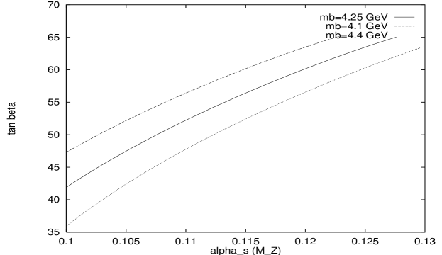
Figure 4: $\tan\beta$ prediction for various values of $\bar{m}_{b}$.

The procedure we follow for the third family is very similar to ref.[3] for bottom-tau Yukawa unification, but are here extended to include full top-bottom-tau Yukawa unification, according to Eq.29. Briefly, the idea is to input $\bar{m}_{b}$, $\bar{m}_{\tau}$ and $\alpha_{S}(M_{Z})$ and then to predict $\bar{m}_{t}$ and $\tan\beta$ as outputs using the constraint of Yukawa unification, as in Eq.29 after running the 3rd family Yukawa couplings up to $M_{X}$. In practice this is complicated by the fact that the Yukawa couplings $\lambda_{t}(\bar{m}_{t})$, $\lambda_{b}(\bar{m}_{t})$, $\lambda_{\tau}(\bar{m}_{t})$ all depend upon the input value of $\bar{m}_{t}$ and $\tan\beta$. Thus we pick reasonable estimates of these quantities to input into the RG routine. The output values obtained from this are fed back as inputs until the iteration converges. In this way we select $\bar{m}_{t}$, $\tan\beta$ consistent for Yukawa unification consistent with given values of $\bar{m}_{b}$, $\bar{m}_{\tau}$, $\alpha_{S}(M_{Z})$. This results in the predictions for $m_{t}$(pole), $\lambda_{33}(M_{X})$ and $\tan\beta$ shown in Figs. 2-4.

As Figs. 2-4 illustrate, the results are highly dependent upon $\alpha_{s}(M_{Z})$, and fairly dependent on $\bar{m}_{b}$. The value of $\tan\beta$ is high (35 to about 65) and $m_{t}($pole$)$ ranges from 130 to 190 GeV. Where the curves on the graphs stop for high $\alpha_{s}(M_{Z})$, one of the couplings has become too high and so the model is not valid in this region of parameter space. Note that for certain superparticle spectrums, these results can be perturbed because the determination of $\bar{m}_{b}(\bar{m}_{b})$ does not include certain one loop Yukawa corrections [12]. This can have the effect of lowering the prediction of $m_{t}$ by about 30 GeV, which is still compatible with the CDF result for higher $\alpha_{s}$.

4.3 First and Second family: Diagonal Yukawa Couplings

In dealing with the first and second families we have to confront the problem that the Yukawa matrices are not diagonal. As discussed widely elsewhere [12, 7], it is most convenient to diagonalise the Yukawa matrices at $M_{X}$ before running them down to $\bar{m}_{t}$. It is then possible to obtain RG equations for both the diagonal Yukawa couplings $\lambda_{u,c,t}$, $\lambda_{d,s,b}$, $\lambda_{e,\mu,\tau}$ and the Cabibbo-Kobayashi-Maskawa (CKM) matrix elements $|V_{ij}|$ (ref.[3]). At one-loop these RG equations can be numerically integrated so that the low energy physical couplings have a simple scaling behaviour [12]:

Figure 5: $I_{f}$ for the third family, as defined in eq.32. The lower (upper) triplet of curves is associated with $\bar{m}_{b}$ = 4.1 (4.4) GeV.

$$\left(\frac{\lambda_{u,c}}{\lambda_{t}}\right)_{\bar{m}_{t}} = \left(\frac{\lambda_{u,c}}{\lambda_{t}}\right)_{M_{X}}e^{3I_{t}+I_{b}}$$

$$\left(\frac{\lambda_{d,s}}{\lambda_{b}}\right)_{\bar{m}_{t}} = \left(\frac{\lambda_{d,s}}{\lambda_{b}}\right)_{M_{X}}e^{3I_{b}+I_{t}}$$

$$\left(\frac{\lambda_{e,\mu}}{\lambda_{\tau}}\right)_{\bar{m}_{t}} = \left(\frac{\lambda_{e,\mu}}{\lambda_{\tau}}\right)_{M_{X}}e^{3I_{\tau}}$$

$$\frac{\mid V_{cb}\mid_{M_{X}}}{\mid V_{cb}\mid_{\bar{m}_{t}}} = e^{I_{b}+I_{t}},$$ (31)

with identical scaling behaviour to $V_{cb}$ of $V_{ub}$, $V_{ts}$, $V_{td}$, where

$$I_{i}=\int_{\ln\bar{m}_{t}}^{\ln{M_{X}}}\left(\frac{\lambda_{i}\left(t\right)}{4\pi}\right)^{2}dt,$$ (32)

and $t=\ln\mu$, $\mu$ being the $\overline{MS}$ scale. To a consistent level of approximation $V_{us}$, $V_{ud}$, $V_{cs}$, $V_{cd}$, $V_{tb}$, $\lambda_{u}$/$\lambda_{c}$, $\lambda_{d}$/$\lambda_{s}$ and $\lambda_{e}$/$\lambda_{\mu}$ are RG invariant. The CP violating quantity J scales as $V_{cb}^{2}$. The $I$ integrals of the third family are displayed in Fig.5 for the allowed range of $\bar{m}_{b}$ and $\alpha_{S}(M_{Z})$.

Figure 6: Empirically derived ratios of first and second to third family lepton Yukawa couplings at $M_{X}$ for $\bar{m}_{b}=4.25$ GeV.

Using Eqs.24-26 we may determine the diagonal Yukawa couplings in this model at $\bar{m}_{t}$. The third family Yukawa couplings at $M_{X}$ (all equal) are given by Fig.3. The first and second family diagonal Yukawa couplings at $M_{X}$ are then easily obtained from the scaling relations in Eq.31, using the $I_{f}$ integrals in Fig.5. These GUT scale Yukawa couplings expressed as ratios are shown in Figs. 6,7,8. The relative magnitude of the diagonal Yukawa couplings between the first two families and the third is displayed in Fig.6, where the ratio should be $O(\epsilon)$ for the first family and $O(\epsilon^{2})$ for the second, if the assumption of suppression of the mass scales is to be correct. As seen in the figure, this identifies $\log(\epsilon)\sim O(-1.5)$.

Figure 7: Empirical bounds on ratios of diagonal Yukawa couplings of the second family at $M_{X}$ and $\bar{m}_{b}=$ 4.25 GeV.

The second family couplings at $M_{X}$ are shown in Fig.7 and show that $\lambda_{s}:\lambda_{\mu}:\lambda_{c}\sim 6:20:1$. The first family couplings are displayed in Fig.8 and give $\lambda_{d}:\lambda_{e}:\lambda_{u}\sim 3:1:1/30$. These are the patterns that must be replicated by our model if it going to be phenomenologically viable. In Fig.9 we also show the absolute value of $|V_{cb}|$ at $M_{X}$, calculated by running the value at $M_{Z}$ in Eq.27 up to $M_{X}$ using Eq.31.

Figure 8: Empirical bounds on ratios of diagonal Yukawa couplings of the first family at $M_{X}$ using $\bar{m}_{b}=4.25$ GeV.

4.4 The Lower 2 by 2 Block of The Yukawa Matrix: The Prediction of the Strange Quark Mass

The heavy 2 by 2 sectors of the Yukawa matrices are considered first, in isolation from the rest of the Yukawa matrix. This is possible because we shall assume that the Yukawa matrices at $M_{X}$ are all of the form

$$Y^{U,D,E}=\left(\begin{array}[]{ccc}O(\epsilon^{2})&O(\epsilon^{2})&0\\ O(\epsilon^{2})&O(\epsilon)&O(\epsilon)\\ 0&O(\epsilon)&O(1)\\ \end{array}\right),$$ (33)

where $\epsilon<<1$ and some of the elements may have approximate or exact texture zeroes in them. Assuming the form Eq.33 allows us to consider the lower 2 by 2 block of the Yukawa matrices first. In diagonalising the lower 2 by 2 block separately, we introduce corrections of order $\epsilon^{2}$ and so the procedure is consistent to first order in $\epsilon$.

In searching for the minimum number of operators that fit phenomenological constraints (so that maximum predictivity is attained) there are some general arguments that yield a lower bound on the number of operators. It is clear that there must be at least 3 operators in the lower 2 by 2 block since it should have no zero rows or columns, or its determinant would be zero, implying that it contains a zero eigenvalue and therefore a zero mass. Also, for a non-zero $|V_{cb}|$, we require there to be an operator in the 32 position in the down and/or up matrices. In fact we shall require 4 operators in the lower 2 by 2 block since the Clebsch coefficients listed in Table 3 are not sufficient to describe successfully all the features of Fig.7, in particular the charm-muon splitting ($\lambda_{\mu}$/$\lambda_{c}\sim 18)$. With 3 operators, excluding the third family discussed previously, we have three Yukawa coupling parameters, not including the 33 coupling which is already calculated. There are four observables connected with these parameters, $|V_{cb}|$, $m_{s}$, $m_{c}$ and $m_{\mu}$. We use $|V_{cb}|,\bar{m}_{c},\bar{m}_{\mu}$ as inputs but the only prediction we can make is for the strange mass $\bar{m}_{s}$.

Figure 9: $|V_{cb}|$ calculated at $M_{X}$ from the low energy value.

Given the constraints listed above, the only ansatze that successfully satisfy them are listed here:

$$A_{1} = \left[\begin{array}[]{cc}O^{D}-O^{C}&0\\ O^{B}&O_{33}\end{array}\right]$$ (36)

$$A_{2} = \left[\begin{array}[]{cc}0&O^{A}-O^{B}\\ O^{D}&O_{33}\end{array}\right]$$ (39)

$$A_{3} = \left[\begin{array}[]{cc}0&O^{C}-O^{D}\\ O^{B}&O_{33}\end{array}\right]$$ (42)

$$A_{4} = \left[\begin{array}[]{cc}0&O^{C}\\ O^{A}-O^{B}&O_{33}\end{array}\right]$$ (45)

$$A_{5} = \left[\begin{array}[]{cc}0&O^{A}\\ O^{C}-O^{D}&O_{33}\end{array}\right]$$ (48)

$$A_{6} = \left[\begin{array}[]{cc}O^{K}&O^{C}\\ O^{M}&O_{33}\end{array}\right]$$ (51)

$$A_{7} = \left[\begin{array}[]{cc}O^{K}&O^{G}\\ O^{G}&O_{33}\end{array}\right]$$ (54)

$$A_{8} = \left[\begin{array}[]{cc}0&O^{H}\\ O^{G}-O^{K}&O_{33}\end{array}\right].$$ (57)

Note that $O^{D}$ can be used in the 32 position of $A_{1}$ instead of $O^{B}$, yielding exactly the same results. Also, ansatze replacing $O^{C}$ with $O^{D}$ in $A_{4}$, $O^{A}$ with $O^{B}$ in $A_{5}$, $O^{K}$ with $O^{N}$ or $O^{O}$ in $A_{6-8}$ and $O^{C}$ with $O^{D}$ in $A_{6,7}$ also yield the same results. $A_{7}$ may be transposed to yield the same results, as may $A_{6}$ if $O^{C}$ is not in the 23 position before transposing, as this would predict zero $|V_{ub}|$.

From the above ansatze in Eqs.36-57, the ratio of muon to strange Yukawa couplings at $M_{X}$ is found to be:

$$\left(\frac{\lambda_{\mu}}{\lambda_{s}}\right)_{M_{X}}\equiv l.$$ (58)

where $l$ is a ratio of Clebsch coefficients, predicted to be $l=3$ (as in the GJ ansatz) or $l=4$ (a new prediction).

Ansatze $A_{1-6}$ predict $l=3$ in Eq.58 and ansatze $A_{7,8}$ predict $l=4$.

Figure 10: $\bar{m}_{s}$(1 GeV) predictions as a result of Eq.58, to be compared with the experimental value quoted in Table 5.

Eq.58 gives a prediction of the quantity $\lambda_{s}(M_{X})$, which can in turn be run down to 1 GeV, yielding a prediction for $\bar{m}_{s}$. Fig.10 shows the predictions for $\bar{m}_{s}$(1 GeV), which were found to have negligible dependence upon $\bar{m}_{b}$. Note that the $l=4$ curve in Fig.10 corresponding to ansatze $A_{7,8}$ works just as well as the $l=3$ GJ prediction.

4.5 The Upper 2 by 2 Block of The Yukawa Matrix: The Prediction of the Down Quark Mass.

Having diagonalised the lower 2 by 2 block, we have an effective Yukawa coupling in the 22 position for each of the Yukawa matrices. We must now add additional operators to account for $m_{e},m_{u},m_{d},|V_{ub}|$ and $|V_{us}|$. We shall assume that these additional operators are $n=2$ ones, as discussed previously together with even smaller $n=3$ operators which we denote generically $O^{n=3}$. Naively the minimum number of additional operators in the upper 2 by 2 block is 2: one in the 21 position to account for $|V_{us}|$ and one on the top row to avoid a massless first family. However, it is impossible to account for $(\lambda_{u}/\lambda_{e})_{M_{X}}\sim 1/30$ and $(\lambda_{u}/\lambda_{d})_{M_{X}}\sim 1/100$ using only two operators, since the magnitude of the Clebsch coefficients in Table 3 are simply not big enough. To circumvent this problem we shall use the operators in Table 3 which give a zero contribution to the up mass and a non zero contribution to the down and electron mass, namely $O^{1,2,3}$. In order to achieve a non-zero $|V_{ub}|$ we require an operator in the 21 position which gives a non-zero contribution to the up-matrix. To provide a phenomenologically viable $|V_{ub}|$ it turns out (see later) that the Clebsch of the down Yukawa coupling in the 21 position has to be 3 times that of the up Yukawa coupling in the 21 position. This implies that the 21 operator must be one of $O^{Ad},O^{Dd}$ or $O^{Md}$. If the 12 operator is simply $O^{1,2,3}$ then this predicts a massless up quark. In order to obtain a small up quark mass we must add a small third operator (denoted $O^{n=3}$) to the 11 or 12 positions. This leads to the successful upper 2 by 2 block ansatze shown below. With three extra operators in the upper block we have three Yukawa coupling parameters, connected with the 5 observables $|V_{us}|,m_{u},m_{d},m_{e}$ and $|V_{ub}|$. $m_{u}$, $m_{e}$ and $|V_{us}|$ are used as inputs and $m_{d},|V_{ub}|$ are predicted.

The possible ansatze in the down sector that account for correct $|V_{us}|,m_{u},m_{d},m_{e}$ and $|V_{ub}|$ and also generate CP violation are:

$$B_{1} = \left[\begin{array}[]{cc}0&O^{n=3}+O^{1}\\ O^{Ad}&X\end{array}\right]$$ (61)

$$B_{2} = \left[\begin{array}[]{cc}0&O^{n=3}+O^{2}\\ O^{Ad}&X\end{array}\right]$$ (64)

$$B_{3} = \left[\begin{array}[]{cc}0&O^{n=3}+O^{3}\\ O^{Ad}&X\end{array}\right]$$ (67)

$$B_{4} = \left[\begin{array}[]{cc}0&O^{n=3}+O^{1}\\ O^{Dd}&X\end{array}\right]$$ (70)

$$B_{5} = \left[\begin{array}[]{cc}0&O^{n=3}+O^{2}\\ O^{Dd}&X\end{array}\right]$$ (73)

$$B_{6} = \left[\begin{array}[]{cc}0&O^{n=3}+O^{3}\\ O^{Dd}&X\end{array}\right]$$ (76)

$$B_{7} = \left[\begin{array}[]{cc}0&O^{n=3}+O^{1}\\ O^{Md}&X\end{array}\right]$$ (79)

$$B_{8} = \left[\begin{array}[]{cc}0&O^{n=3}+O^{2}\\ O^{Md}&X\end{array}\right].$$ (82)

$X$ stands for whatever is left in the 22 position, after the lower 2 by 2 submatrix has been diagonalised. Each of the successful ansatze gives a prediction for the down Yukawa coupling at $M_{X}$ in terms of the electron Yukawa coupling:

$$\left(\frac{\lambda_{d}}{\lambda_{e}}\right)_{M_{X}}\equiv k,$$ (83)

where $k=3$ is the Georgi–Jarlskog prediction of $\bar{m}_{d}$. Other viable possibilities found in our analysis are $k=2,4,\frac{8}{3},\frac{16}{3}$ as shown in Table 7. The $k$ values as defined in Eq.83 depend upon the $l$ value in the heavy submatrix and are displayed in Table 7.

$k$	$B_{1}$	$B_{2}$	$B_{3}$	$B_{4}$	$B_{5}$	$B_{6}$	$B_{7}$	$B_{8}$
$A_{1-6}$	4	16/3	2	3	4	(3/2)	(3/2)	2
$A_{7,8}$	16/3	(64/9)	8/3	4	16/3	2	2	8/3

Table 7: $k$ values predicted by the ansatze $A_{1}$ to $A_{8}$ when combined with $B_{1}$ to $B_{8}$. Note that the bracketed entries predict $\bar{m}_{d}(1$ GeV$)$ to be outside the empirical range, and so are not included in Fig.11.

Figure 11: $\bar{m}_{d}$(1 GeV) prediction as a result of the Eq.83, with the $k$ values outlined in Table 7, labeling each prediction.

Fig.11 shows the five possible predictions for $\bar{m}_{d}$ in the separate ansatze. Again, the results were found to have negligible dependence on $\bar{m}_{b}$ because this will only change the RG running by affecting $\bar{m}_{t}$. The large $\tan\beta$ dependence factors out since we relate the mass of the down quarks to the mass of the leptons only, and these have the same dependence upon $\tan\beta$. It should be made clear that up until now all of the Yukawa couplings are assumed to be real and positive, but in order to do a full analysis of the CKM matrix including the CP violating phase we shall now drop this assumption.

4.6 The Full 3 by 3 Yukawa Matrix: The Prediction of $|V_{ub}|$ in Terms of the CP-Violating Phase

So far we have discussed the lower 2 by 2 block and the upper 2 by 2 block of the Yukawa matrices, assuming them to be of the form shown in Eq.33, and taking all of the couplings to be real and positive. In fact the effective Yukawa couplings must be regarded as complex parameters with relative phases between them. This does not affect our analysis of third family Yukawa unification. Nor does it affect the predictions of the strange and down quark masses which follow from Eqs.83,58, since $l$ and $k$ are simply ratios of Clebsch coefficients. However the precise list of successful lower 2 by 2 block ansatze $A_{i}$ in section 4.4, and the upper 2 by 2 block ansatze $B_{i}$ in section 4.5 was in fact based on a full analysis of the 3 by 3 Yukawa matrices, including complex phases. We shall not repeat the full analysis which led to the successful ansatze $A_{i}$ and $B_{i}$ here. However in order to illustrate our approach and discuss the remaining CKM parameters, it is instructive to consider one example as described below.

The successful ansatze consist of any of the lower 2 by 2 blocks $A_{i}$ combined with any of the upper 2 by 2 blocks $B_{i}$, subject to the restrictions shown in Table 7. For example let us consider $A_{1}$ in the lower 2 by 2 block combined with any of the $B_{i}$ in the upper 2 by 2 block, focusing particularly on $A_{1}$ combined with $B_{1}$. Just above $M_{X}$, before the $H,\bar{H}$ fields develop VEVs, we have the operators

$$\left[\begin{array}[]{ccc}0&O^{1}_{12}+{O}_{12}^{n=3}&0\\ O^{Ad}_{21}&O^{D}_{22}-{O}^{C}_{22}&0\\ 0&O^{B}_{32}&O_{33}\\ \end{array}\right],$$ (84)

which implies that at $M_{X}$ the Yukawa matrices are of the form

$$Y^{U,D,E}=\left[\begin{array}[]{ccc}0&H_{12}x_{12}^{U,D,E}e^{i\phi_{12}}+H_{12}{{}^{\prime}}x{{}^{\prime}}_{12}^{U,D,E}e^{i\phi_{12}^{\prime}}&0\\ H_{21}x_{21}^{U,D,E}e^{i\phi_{21}}&H_{22}x_{22}^{U,D,E}e^{i\phi_{22}}-H_{22}^{\prime}x_{22}^{\prime U,D,E}e^{i\phi_{22}^{\prime}}&0\\ 0&H_{32}x_{32}^{U,D,E}e^{i\phi_{32}}&H_{33}e^{i\phi_{33}}\\ \end{array}\right],$$ (85)

where we have factored out the phases of the operators and $H_{ik}$ are the magnitudes of the coupling constant associated with $O_{ik}$. Note the real Clebsch coefficients $x_{ik}^{U,D,E}$ give the splittings between $Y^{U,D,E}$. In our particular case $A_{1},B_{1}$ they are given by

$$x_{12}^{U}=0 x_{12}^{D}=1 x_{12}^{E}=1$$

$$x_{21}^{U}=1 x_{21}^{D}=3 x_{21}^{E}=9/4$$

$$x_{22}^{U}=1 x_{22}^{D}=-1 x_{22}^{E}=3$$

$${x^{\prime}}_{22}^{U}=1 {x^{\prime}}_{22}^{D}=1 {x^{\prime}}_{22}^{E}=-3$$

$$x_{32}^{U}=1 x_{32}^{D}=-1 x_{32}^{E}=-1$$ (86)

and ${x^{\prime}}_{12}^{U}\neq 0$. We now make the transformation in the 22 element of Eq.85

$$x_{22}^{U}H_{22}e^{i\phi_{22}}-x{{}^{\prime}}_{22}^{U}H_{22}^{\prime}e^{i\phi^{\prime}_{22}} \equiv H_{22}^{U}e^{i\phi_{22}^{U}}$$

$$x_{22}^{D}H_{22}e^{i\phi_{22}}-x{{}^{\prime}}_{22}^{D}H_{22}^{\prime}e^{i\phi^{\prime}_{22}} \equiv H_{22}^{D}e^{i\phi_{22}^{D}}$$

$$x_{22}^{E}H_{22}e^{i\phi_{22}}-x{{}^{\prime}}_{22}^{E}H_{22}^{\prime}e^{i\phi^{\prime}_{22}} \equiv H_{22}^{E}e^{i\phi_{22}^{E}},$$ (87)

where $H_{22}^{U,D,E},\phi_{22}^{U,D,E}$ are real positive parameters. It follows from the Clebsch structure in Eq.86 that $H_{22}^{E}=3H_{22}^{D}$ and $\phi_{22}^{E}=\phi_{22}^{D}$. In general we shall write $H_{22}^{E}=lH_{22}^{D}$, where $l=3$ in this case.

At $M_{X}$, we have the freedom to rotate the phases of $F^{i}$ and $\bar{F}_{j}$, since this leaves the lagrangian of the high energy theory invariant. In doing this we rotate away 5 phases in the matrices since there are only 5 relative phases:

$$\left[\begin{array}[]{c}\bar{F}_{1}\\ \bar{F}_{2}\\ \bar{F}_{3}\end{array}\right] \rightarrow \left[\begin{array}[]{ccc}e^{-i(\phi_{32}-\phi_{12})}&0&0\\ 0&e^{-i(\phi_{32}-\phi_{22}^{D})}&0\\ 0&0&1\\ \end{array}\right]\left[\begin{array}[]{c}\bar{F}_{1}\\ \bar{F}_{2}\\ \bar{F}_{3}\end{array}\right]$$ (97)

$$\left[\begin{array}[]{c}F_{1}\\ F_{2}\\ F_{3}\end{array}\right] \rightarrow \left[\begin{array}[]{ccc}e^{-i(-\phi_{32}+\phi_{22}^{D}-\phi_{21})}&0&0\\ 0&e^{i\phi_{32}}&0\\ 0&0&e^{i\phi_{33}}\\ \end{array}\right]\left[\begin{array}[]{c}F_{1}\\ F_{2}\\ F_{3}\end{array}\right].$$ (107)

Below $M_{X}$, the multiplets $F,\bar{F}$ are no longer connected by the gauge symmetry in the effective field theory, since it is The Standard Model. We now define our notation as regards the effective field theory below $M_{X}$ as follows. The effective quark Yukawa terms are written (suppressing all indices)

$$(U_{R})^{c}Y^{U}Q_{L}h_{2}+(D_{R})^{c}Y^{D}Q_{L}h_{1}+H.c.$$ (108)

We transform to the quark mass basis by introducing four 3 by 3 unitary matrices $V_{U_{L,R}},V_{D_{L,R}}$ then the Yukawa terms become

$$(U_{R})^{c}V_{U_{R}}^{\dagger}V_{U_{R}}Y^{U}V_{U_{L}}^{\dagger}V_{U_{L}}Q_{L}h_{2}+(D_{R})^{c}V_{D_{R}}^{\dagger}V_{D_{R}}Y^{D}V_{D_{L}}^{\dagger}V_{D_{L}}Q_{L}h_{1}+H.c.$$ (109)

where $Y^{U}_{\mbox{diag}}=V_{U_{R}}Y^{U}V_{U_{L}}^{\dagger}$ and $Y^{D}_{\mbox{diag}}=V_{D_{R}}Y^{D}V_{D_{L}}^{\dagger}$ are the diagonalised Yukawa matrices. With the definitions in Eqs.108,109, the CKM matrix is of the form

$$V_{CKM}\equiv V_{U_{L}}V_{D_{L}}^{\dagger}.$$ (110)

In all of the cases considered, $x_{12}^{U}=0$ and $x_{12}^{\prime D,E}=0$ so that the Yukawa matrices which result from Eqs.85,87,107 are

$$Y^{D} = \left[\begin{array}[]{ccc}0&H_{12}x_{12}^{D}&0\\ H_{21}x_{21}^{D}&H_{22}^{D}&0\\ 0&H_{32}x_{32}^{D}&H_{33}\\ \end{array}\right]$$ (114)

$$Y^{E} = \left[\begin{array}[]{ccc}0&H_{12}x_{12}^{E}&0\\ H_{21}x_{21}^{E}&lH_{22}^{D}&0\\ 0&H_{32}x_{32}^{E}&H_{33}\\ \end{array}\right]$$ (118)

$$Y^{U} = \left[\begin{array}[]{ccc}0&H_{12}^{\prime}{x^{\prime}}^{U}_{12}e^{i(\phi_{12}{{}^{\prime}}-\phi_{12})}&0\\ x_{21}^{U}H_{21}&H_{22}^{U}e^{i(\phi_{22}^{U}-\phi_{22}^{D})}&0\\ 0&H_{32}x_{32}^{U}&H_{33}\\ \end{array}\right].$$ (122)

In order to diagonalise the quark Yukawa matrices, we first make $Y^{U}$ real, by multiplying by phase matrices

$$Y^{U}\rightarrow\left[\begin{array}[]{ccc}e^{i\bar{\phi}_{12}}&0&0\\ 0&e^{i\bar{\phi}_{22}}&0\\ 0&0&1\\ \end{array}\right] Y^{U} \left[\begin{array}[]{ccc}e^{i\bar{\phi}_{22}^{U}}&0&0\\ 0&1&0\\ 0&0&1\\ \end{array}\right],$$ (129)

where we have defined $\bar{\phi}_{22}\equiv\phi_{22}^{U}-\phi_{22}^{D}$ and $\bar{\phi}_{12}\equiv\phi_{12}^{\prime}-\phi_{12}$. This amounts to a phase redefinition of the $(U_{R})^{c}$ and $U_{L}$ fields.

To diagonalise the real matrices obtained from the above phase rotations, we first diagonalise the heavy 2 by 2 submatrices, then the light submatrices as shown below,

$$Y^{D}\rightarrow\left[\begin{array}[]{ccc}\tilde{c}_{2}&\tilde{s}_{2}&0\\ -\tilde{s}_{2}&\tilde{c}_{2}&0\\ 0&0&1\end{array}\right]\left[\begin{array}[]{ccc}1&0&0\\ 0&\tilde{c}_{4}&\tilde{s}_{4}\\ 0&-\tilde{s}_{4}&\tilde{c}_{4}\\ \end{array}\right] Y^{D} \left[\begin{array}[]{ccc}1&0&0\\ 0&\bar{c}_{4}&-\bar{s}_{4}\\ 0&\bar{s}_{4}&\bar{c}_{4}\\ \end{array}\right]\left[\begin{array}[]{ccc}c_{2}&-s_{2}&0\\ s_{2}&c_{2}&0\\ 0&0&1\\ \end{array}\right]$$ (142)

$$Y^{U}\rightarrow\left[\begin{array}[]{ccc}\tilde{c}_{1}&\tilde{s}_{1}&0\\ -\tilde{s}_{1}&\tilde{c}_{1}&0\\ 0&0&1\end{array}\right]\left[\begin{array}[]{ccc}1&0&0\\ 0&\tilde{c}_{3}&\tilde{s}_{3}\\ 0&-\tilde{s}_{3}&\tilde{c}_{3}\\ \end{array}\right] Y^{U} \left[\begin{array}[]{ccc}1&0&0\\ 0&\bar{c}_{3}&-\bar{s}_{3}\\ 0&\bar{s}_{3}&\bar{c}_{3}\\ \end{array}\right]\left[\begin{array}[]{ccc}c_{1}&-s_{1}&0\\ s_{1}&c_{1}&0\\ 0&0&1\\ \end{array}\right],$$ (155)

where $c_{i},\bar{s}_{i}$ refer to $\cos\theta_{i}$ and $\sin\bar{\theta}_{i}$ respectively. Note that since $Y^{U,D}$ are not symmetric $\tilde{c}_{i},\tilde{s}_{i}$ are independent of $c_{i},\bar{s}_{i}$.

The diagonal Yukawa couplings of the strange quark and muon obtained from Eq.155 are $(\lambda_{s})_{M_{X}}=H_{22}^{D}$ and $(\lambda_{\mu})_{M_{X}}=lH_{22}^{D}$ since the 22 eigenvalues are just the 22 elements in this case. The first family diagonal Yukawa couplings for the down quark and electron are related by

$$\left(\frac{\lambda_{d}}{\lambda_{e}}\right)_{M_{X}}=l\frac{x_{21}^{D}x_{12}^{D}}{x_{21}^{E}x_{12}^{E}}.$$ (156)

We identify the right hand side of Eq.156 with $k$ in Eq.83. The angles are given by $\bar{s}_{4}=-x_{32}^{D}H_{32}/H_{33}$, $s_{2}=-x_{21}^{D}H_{21}/(\lambda_{s})_{M_{X}}$, $s_{1}=-x_{21}^{U}H_{21}/(\lambda_{c})_{M_{X}}$ and $\bar{s}_{3}=-x^{U}_{32}H_{32}/H_{33}$. Note that $(\lambda_{u})_{M_{X}}=-{x^{\prime}}_{12}^{U}x_{21}^{U}H_{12}^{\prime}H_{21}/(\lambda_{c})_{M_{X}}$ is small and in the limit ${O_{12}}^{\prime}\rightarrow 0$ the up quark is massless in the model.

Figure 12: $|V_{ub}|$ bounds predicted in terms of the complex phase $\phi$ for various $\alpha_{s}(M_{Z})$ and the ansatze $A_{1-6}$, corresponding to $l=3$.

Denoting $\theta_{3}=\bar{\theta}_{3}-\bar{\theta}_{4}$ and $\phi=-\bar{\phi}_{22}$ , we substitute the diagonalising matrices from Eqs. 155 and 129 into the CKM matrix in Eq.110 to obtain

$$V_{CKM}=\left[\begin{array}[]{ccc}c_{2}c_{1}e^{i\phi}+s_{2}s_{1}c_{3}&-s_{2}c_{1}e^{i\phi}+s_{1}c_{2}c_{3}&s_{1}s_{3}\\ -s_{1}c_{2}e^{i\phi}+c_{1}s_{2}c_{3}&s_{1}s_{2}e^{i\phi}+c_{2}c_{3}c_{1}&s_{3}c_{1}\\ -s_{2}s_{3}&-c_{2}s_{3}&c_{3}\end{array}\right].$$ (157)

Note that $\tan\theta_{1}=\frac{V_{ub}}{V_{cb}}$. This is a generic feature of all the ansatze. To obtain a prediction for $|V_{ub}|$ we note that

$$|V_{us}| = |-s_{2}c_{1}e^{i\phi}+s_{1}c_{2}c_{3}|$$

$$\sim |\frac{V_{ub}}{V_{cb}}||\frac{x_{21}^{D}\lambda_{c}}{x_{21}^{U}\lambda_{s}}e^{i\phi}-1|$$

$$\Rightarrow|V_{ub}(m_{t})| \sim \frac{|V_{us}(m_{t})||V_{cb}(m_{t})|}{\sqrt{1+\left(\frac{x_{21}^{D}\lambda_{c}(M_{X})}{x_{21}^{U}\lambda_{s}(M_{X})}\right)^{2}-2\cos\phi(M_{X})\frac{x_{21}^{D}\lambda_{c}(M_{X})}{x_{21}^{U}\lambda_{s}(M_{X})}}}.$$ (158)

Eq.158 predicts a value of $|V_{ub}|$ that is dependent upon the value of $l$. This is because of the appearance of $\lambda_{s}$ in Eq.158, which is predicted to have different values in Eq.58 depending on $l$. The $|V_{ub}|$ predicted is displayed in Figs. 12 and 13 and fits the phenomenological values of 0.002–0.005 successfully only for large values of the complex phase. Clearly Figs.12,13 predict large values of $|V_{ub}|$. We emphasise that this prediction applies to all of the successful ansatze $A_{i},B_{i}$.

Figure 13: $|V_{ub}|$ bounds predicted in terms of the complex phase $\phi$ for various $\alpha_{s}(M_{Z})$ and the ansatze $A_{7,8}$, corresponding to $l=4$.

5 Conclusions

We have discussed the problem of fermion masses in the supersymmetric SU(4)$\otimes$ SU(2)${}_{L}\otimes$SU(2)_R model, where the gauge group is assumed to be broken to the standard gauge group at $M_{X}\sim 10^{16}$ GeV. Although the gauge group is not unified at $M_{X}$, it is hoped that the model may be embedded in some string theory near the Planck scale. Since the model involves no adjoint representations of the gauge group, and has no doublet-triplet splitting problem, the prospects for achieving string unification in this model are very good, and some attempts in this direction have already been made [10]. However here we have restricted ourselves to the low-energy effective field theory near the scale $M_{X}\sim 10^{16}$ GeV, and parameterised the effects of string unification by non-renormalisable operators whose coefficients are suppressed by powers of $(M_{X}/M)$, where $M>M_{X}$ is some higher scale associated with string physics.

We have assumed that the heavy third family receives its mass from a single renormalisable Yukawa coupling in the superpotential. The model predicts third family Yukawa unification (i.e. the top, bottom and tau Yukawa couplings are all equal at $M_{X}$) leading to predictions for the top mass and $\tan\beta$. The other Yukawa couplings result from the effect of non-renormalisable operators of order $(M_{X}/M)^{2n}$, where $n=1$ operators are suitable for the lower 2 by 2 block of the Yukawa matrices, and $n=2,3$ are suitable for the upper 2 by 2 block. In fact we have classified all possible operators in this model for $n=1$ and $n=2$.

The successful ansatz $A_{i},B_{i}$ in Eqs.36-57,61-82 involve 8 real parameters $H_{33}$, $H_{32}$, $H_{22}^{U,D}$, $H_{21}$, $H_{12}$, $H_{12}^{\prime}$, plus an unremovable phase. With these 8 parameters we can describe the 13 physical quantities $\bar{m}_{u}$, $\bar{m}_{d}$, $\bar{m}_{s}$, $\bar{m}_{c}$, $\bar{m}_{b}$, $\bar{m}_{t}$, $\bar{m}_{e}$, $\bar{m}_{\mu}$, $\bar{m}_{\tau}$, $\theta_{1,2,3}$, $\phi$. Third family Yukawa unification led to a prediction for $m_{t}(\mbox{pole})=130-200$ GeV and $\tan\beta=35-65$, depending on $\alpha_{S}(M_{Z})$ and $\bar{m}_{b}$. More accurate predictions could be obtained if the error on $\alpha_{S}(M_{Z})$ and $\bar{m}_{b}$ were reduced. The analysis of the lower 2 by 2 block led to 2 possible predictions for $\bar{m}_{s}$ depending on whether $l=3$ or $4$, as shown in Fig.10 ($l=3$ is the GJ prediction). In the upper 2 by 2 block analysis we were led to 5 possible predictions for $\bar{m}_{d}$, depending on whether $k=2,8/3,3,4,16/3$, as shown in Fig.11 (again $k=3$ is the GJ prediction.) Finally, we have 2 predictions for $|V_{ub}|$ depending on whether $l=3$ or 4, as shown in Figs.12,13. Both predict a large value of $|V_{ub}|$, depending on $\phi$.

The high values of $\tan\beta$ required by our model (also predicted in SO(10)) can be arranged by a suitable choice of soft SUSY breaking parameters as discussed in ref.[25], although this leads to a moderate fine tuning problem [16]. The high value of $\tan\beta$ is not stable under radiative corrections unless some other mechanism such as extra approximate symmetries are invoked. $m_{t}$ may have been overestimated, since for high $\tan\beta$, the equations for the running of the Yukawa couplings in the MSSM can get corrections of a significant size from Higgsino–stop and gluino–sbottom loops. The size of this effect depends upon the mass spectrum and may be as much as 30 GeV. For our results to be quantitatively correct, the sparticle corrections to $m_{b}$ must be small. This could happen in a scenario with non-universal soft parameters, for example. Not included in our analysis are threshold effects, at low or high energies. These could alter our results by several per cent and so it should be borne in mind that all of the mass predictions have a significant uncertainty in them. It is also unclear how reliable 3 loop perturbative QCD at 1 GeV is.

Compared to SO(10) [12], the lack of predictivity of our model is somewhat discouraging. In the SO(10) model, the spectrum is described by just 4 operators, whereas in our model the spectrum is described by 7 operators. One basic reason for this is that, unlike SO(10), our Yukawa matrices are inherently asymmetric. In order to fill out our Yukawa matrices, we need to add operators in the $ij$ and $ji$ positions separately. This of course permits asymmetric texture zeroes such as those in $A_{1-8}$, which have not been studied before. In the upper 2 by 2 block, the SO(10) model can satisfy all of the phenomenological constraints with just 2 operators, the up Yukawa coupling becoming very small through a small Clebsch ratio $(1/27)^{2}$. This permits the SO(10) model to make predictions for the up quark mass and the complex phase as well as $|V_{ub}|$. Whereas we cannot predict $\bar{m}_{u}$ in this model, a natural explanation is given for its relatively small value in terms of a higher dimensional operator. Note that simply not having this operator would not alter any of the predictions, except that the up quark would be massless, thus solving the strong CP problem. Thus a simple and natural way of obtaining a massless up quark is given by our model with $O^{n=3}\rightarrow 0$ in Eqs. 61-82, which would reduce the number of operators in our model by one.

Despite the lack of predictivity of the model compared to SO(10), the SU(4) $\otimes$SU(2)${}_{L}\otimes$SU(2)_R model has the twin advantages of having no doublet-triplet splitting problem, and containing no adjoint representations, making the model technically simpler to embed into a realistic string theory. Although both these problems can be addressed in the SO(10) model [26, 27], we find it encouraging that such problems do not arise in the first place in the SU(4)$\otimes$SU(2)${}_{L}\otimes$SU(2)_R model. Of course there are other models which also share these advantages such as flipped SU(5) or even the standard model. However, at the field theory level, such models do not lead to Yukawa unification, or have precise Clebsch relations between the operators describing the light fermion masses. It is the combination of all of the attractive features mentioned above which singles out the present model for serious consideration.

Acknowledgments

B. C. Allanach would like to thank PPARC for financial support in the duration of this work.

Appendix 1 : $n=1$ Operators

Following is a list of all $n=1$ non–renormalisable operators. These operators are constructed from various group theoretic contractions of the following five fields,

$$O^{\alpha\rho yw}_{\beta\gamma xz}=F^{\alpha a}\bar{F}_{\beta x}h^{y}_{a}\bar{H}_{\gamma z}H^{\rho w}.$$ (159)

It is useful to define some SU(4) invariant tensors $C$, and SU(2)_R invariant tensors $R$ as follows:

$$(C_{1})^{\alpha}_{\beta} = \delta^{\alpha}_{\beta}$$

$$(C_{15})^{\alpha\rho}_{\beta\gamma} = \delta^{\beta}_{\gamma}\delta^{\rho}_{\alpha}-\frac{1}{4}\delta^{\beta}_{\alpha}\delta^{\rho}_{\gamma}$$

$$(C_{6})_{\alpha\beta}^{\rho\gamma} = \epsilon_{\alpha\beta\omega\chi}\epsilon^{\rho\gamma\omega\chi}$$

$$(C_{10})^{\alpha\beta}_{\rho\gamma} = \delta^{\alpha}_{\rho}\delta^{\beta}_{\gamma}+\delta^{\alpha}_{\gamma}\delta^{\beta}_{\rho}$$

$$(R_{1})^{x}_{y} = \delta^{x}_{y}$$

$$(R_{3})^{wx}_{yz} = \delta^{x}_{y}\delta^{w}_{z}-\frac{1}{2}\delta^{x}_{z}\delta^{w}_{y}$$

$$(R_{S})^{wx}_{yz} = \delta_{y}^{w}\delta_{z}^{x}+\delta^{w}_{z}\delta^{x}_{y},$$ (160)

where $\delta^{\alpha}_{\beta}$, $\epsilon_{\alpha\beta\omega\chi}$, $\delta^{x}_{y}$, $\epsilon_{wz}$ are the usual invariant tensors of SU(4), SU(2)_R. The SU(4) indices on $C_{1,6,10,15}$ are contracted with the SU(4) indices on two fields to combine them into $\underline{1}$, $\underline{6}$, $\underline{10}$, $\underline{15}$ representations of SU(4) respectively. Similarly, the SU(2)_R indices on $R_{1,3}$ are contracted with SU(2)_R indices on two of the fields to combine them into $\underline{1}$, $\underline{3}$ representation of SU(2)_R.

The operators in Tables 1,2 are then given explicitly by contracting Eq.159 with the invariant tensors of Eq.160 in the following manner:

$$O^{A} \sim (C_{1})^{\beta}_{\alpha}(C_{1})^{\gamma}_{\rho}(R_{1})^{z}_{w}(R_{1})^{x}_{y}O^{\alpha\rho yw}_{\beta\gamma xz}$$

$$O^{B} \sim (C_{1})^{\beta}_{\alpha}(C_{1})^{\gamma}_{\rho}(R_{3})^{zq}_{wr}(R_{3})^{xr}_{yq}O^{\alpha\rho yw}_{\beta\gamma xz}$$

$$O^{C} \sim (C_{15})^{\beta\chi}_{\alpha\sigma}(C_{15})^{\gamma\sigma}_{\rho\chi}(R_{1})^{z}_{w}(R_{1})^{x}_{y}O^{\alpha\rho yw}_{\beta\gamma xz}$$

$$O^{D} \sim (C_{15})^{\beta\chi}_{\alpha\sigma}(C_{15})^{\gamma\sigma}_{\rho\chi}(R_{3})^{zq}_{wr}(R_{3})^{xr}_{yq}O^{\alpha\rho yw}_{\beta\gamma xz}$$

$$O^{E} \sim (C_{6})^{\omega\chi}_{\alpha\rho}(C_{6})^{\beta\gamma}_{\omega\chi}\epsilon^{zx}\epsilon_{yw}O^{\alpha\rho yw}_{\beta\gamma xz}$$

$$O^{F} \sim (C_{6})^{\omega\chi}_{\alpha\rho}(C_{6})^{\beta\gamma}_{\omega\chi}(R_{3})^{sq}_{wr}(R_{3})^{xr}_{tq}\epsilon_{ys}\epsilon^{zt}O^{\alpha\rho yw}_{\beta\gamma xz}$$

$$O^{G} \sim (C_{10})^{\omega\chi}_{\alpha\rho}(C_{10})^{\beta\gamma}_{\omega\chi}\epsilon^{xz}\epsilon_{yw}O^{\alpha\rho yw}_{\beta\gamma xz}$$

$$O^{H} \sim (C_{10})^{\omega\chi}_{\alpha\rho}(C_{10})^{\beta\gamma}_{\omega\chi}(R_{S})^{xz}_{qr}(R_{S})^{qr}_{yw}O^{\alpha\rho yw}_{\beta\gamma xz}$$

$$O^{I} \sim (C_{1})^{\gamma}_{\alpha}(C_{1})^{\beta}_{\rho}(R_{1})^{z}_{y}(R_{1})^{x}_{w}O^{\alpha\rho yw}_{\beta\gamma xz}$$

$$O^{J} \sim (C_{1})^{\beta}_{\rho}(C_{1})^{\gamma}_{\alpha}(R_{3})^{zq}_{yr}(R_{3})^{xr}_{wq}O^{\alpha\rho yw}_{\beta\gamma xz}$$

$$O^{K} \sim (C_{15})^{\gamma\omega}_{\alpha\chi}(C_{15})^{\beta\chi}_{\rho\omega}(R_{1})^{z}_{y}(R_{1})^{x}_{w}O^{\alpha\rho yw}_{\beta\gamma xz}$$

$$O^{L} \sim (C_{15})^{\gamma\omega}_{\alpha\chi}(C_{15})^{\beta\chi}_{\rho\omega}(R_{3})^{zq}_{yr}(R_{3})^{xr}_{wq}O^{\alpha\rho yw}_{\beta\gamma xz}$$

$$O^{M} \sim (C_{1})^{\beta}_{\alpha}(C_{1})^{\gamma}_{\rho}\epsilon^{zx}\epsilon_{wy}O^{\alpha\rho yw}_{\beta\gamma xz}$$

$$O^{N} \sim (C_{6})^{\omega\chi}_{\alpha\rho}(C_{6})^{\beta\gamma}_{\omega\chi}(R_{1})^{z}_{y}(R_{1})^{x}_{w}O^{\alpha\rho yw}_{\beta\gamma xz}$$

$$O^{O} \sim (C_{10})^{\omega\chi}_{\alpha\rho}(C_{10})^{\beta\gamma}_{\omega\chi}(R_{1})^{z}_{y}(R_{1})^{x}_{w}O^{\alpha\rho yw}_{\beta\gamma xz}$$

$$O^{P} \sim (C_{15})^{\gamma\omega}_{\alpha\chi}(C_{15})^{\beta\chi}_{\rho\omega}(R_{1})^{z}_{w}(R_{1})^{x}_{y}O^{\alpha\rho yw}_{\beta\gamma xz}.$$ (161)

Appendix 2: $n=2$ Operators

The $n=2$ operators are formed from the following seven fields:

$$O^{\rho_{1}\rho_{2}\rho_{3}aoq}_{\gamma_{1}\gamma_{2}\gamma_{3}mpn}=F^{\rho_{1}a}\bar{H}_{\gamma_{1}m}\bar{F}_{\gamma_{2}p}H^{\rho_{2}o}\bar{H}_{\gamma_{3}n}H^{\rho_{3}q}h^{r}_{a}.$$ (162)

Apart from the invariants defined in Eq.160, we also define

$$(C_{20})^{\alpha\beta\gamma}_{\rho\sigma\omega} = \delta^{\alpha}_{\sigma}\delta^{\beta}_{\rho}\delta^{\gamma}_{\omega}+\delta^{\alpha}_{\sigma}\delta^{\beta}_{\omega}\delta^{\gamma}_{\rho}+\delta^{\alpha}_{\rho}\delta^{\beta}_{\omega}\delta^{\gamma}_{\sigma}+\delta^{\alpha}_{\omega}\delta^{\beta}_{\sigma}\delta^{\gamma}_{\rho}+\delta^{\alpha}_{\omega}\delta^{\beta}_{\rho}\delta^{\gamma}_{\sigma}+\delta^{\alpha}_{\rho}\delta^{\beta}_{\sigma}\delta^{\gamma}_{\omega}$$

$$(R_{4})^{mnt}_{bck} = \delta^{m}_{c}\delta^{n}_{b}\delta^{t}_{k}+\delta^{m}_{c}\delta^{n}_{k}\delta^{t}_{b}+\delta^{m}_{b}\delta^{n}_{k}\delta^{t}_{c}+\delta^{m}_{k}\delta^{n}_{c}\delta^{t}_{b}+\delta^{m}_{k}\delta^{n}_{b}\delta^{t}_{c}+\delta^{m}_{b}\delta^{n}_{c}\delta^{t}_{k},$$ (163)

where the possible SU(4) structures which multiply Eq.162 are

$$(A)^{\gamma_{1}\gamma_{2}\gamma_{3}}_{\rho_{1}\rho_{2}\rho_{3}} = (C_{15})^{\gamma_{1}\alpha}_{\rho_{1}\beta}(C_{15})^{\gamma_{2}\beta}_{\rho_{2}\alpha}(C_{1})^{\gamma_{3}}_{\rho_{3}}$$

$$(B)^{\gamma_{1}\gamma_{2}\gamma_{3}}_{\rho_{1}\rho_{2}\rho_{3}} = (C_{15})^{\gamma_{3}\alpha}_{\rho_{3}\beta}(C_{15})^{\gamma_{2}\beta}_{\rho_{2}\alpha}(C_{1})^{\gamma_{1}}_{\rho_{1}}$$

$$(C)^{\gamma_{1}\gamma_{2}\gamma_{3}}_{\rho_{1}\rho_{2}\rho_{3}} = (C_{15})^{\gamma_{1}\alpha}_{\rho_{1}\beta}(C_{15})^{\gamma_{3}\beta}_{\rho_{3}\alpha}(C_{1})^{\gamma_{2}}_{\rho_{2}}$$

$$(D)^{\gamma_{1}\gamma_{2}\gamma_{3}}_{\rho_{1}\rho_{2}\rho_{3}} = (C_{1})^{\gamma_{2}}_{\rho_{1}}(C_{1})^{\gamma_{1}}_{\rho_{2}}(C_{1})^{\gamma_{3}}_{\rho_{3}}$$

$$(E)^{\gamma_{1}\gamma_{2}\gamma_{3}}_{\rho_{1}\rho_{2}\rho_{3}} = (C_{1})^{\gamma_{1}}_{\rho_{1}}(C_{1})^{\gamma_{2}}_{\rho_{2}}(C_{1})^{\gamma_{3}}_{\rho_{3}}$$

$$(F)^{\gamma_{1}\gamma_{2}\gamma_{3}}_{\rho_{1}\rho_{2}\rho_{3}} = (C_{20})^{\alpha\beta\gamma}_{\rho_{1}\rho_{2}\rho_{3}}(C_{20})^{\gamma_{1}\gamma_{2}\gamma_{3}}_{\alpha\beta\gamma}$$

$$(G)^{\gamma_{1}\gamma_{2}\gamma_{3}}_{\rho_{1}\rho_{2}\rho_{3}} = (C_{10})^{\alpha\beta}_{\rho_{1}\rho_{2}}\epsilon_{\alpha\rho_{3}\mu\sigma}(C_{10})^{\gamma_{1}\gamma_{2}}_{\omega\beta}\epsilon^{\omega\gamma_{3}\mu\sigma}$$

$$(H)^{\gamma_{1}\gamma_{2}\gamma_{3}}_{\rho_{1}\rho_{2}\rho_{3}} = (C_{10})^{\alpha\beta}_{\rho_{3}\rho_{2}}\epsilon_{\alpha\rho_{1}\mu\sigma}(C_{10})^{\gamma_{1}\gamma_{2}}_{\omega\beta}\epsilon^{\omega\gamma_{3}\mu\sigma}$$

$$(I)^{\gamma_{1}\gamma_{2}\gamma_{3}}_{\rho_{1}\rho_{2}\rho_{3}} = (C_{10})^{\alpha\beta}_{\rho_{1}\rho_{3}}\epsilon_{\alpha\rho_{2}\mu\sigma}(C_{10})^{\gamma_{1}\gamma_{2}}_{\omega\beta}\epsilon^{\omega\gamma_{3}\mu\sigma}$$

$$(J)^{\gamma_{1}\gamma_{2}\gamma_{3}}_{\rho_{1}\rho_{2}\rho_{3}} = (C_{10})^{\alpha\beta}_{\rho_{1}\rho_{2}}\epsilon_{\alpha\rho_{3}\mu\sigma}(C_{10})^{\gamma_{1}\gamma_{3}}_{\omega\beta}\epsilon^{\omega\gamma_{2}\mu\sigma}$$

$$(K)^{\gamma_{1}\gamma_{2}\gamma_{3}}_{\rho_{1}\rho_{2}\rho_{3}} = (C_{10})^{\alpha\beta}_{\rho_{3}\rho_{2}}\epsilon_{\alpha\rho_{1}\mu\sigma}(C_{10})^{\gamma_{1}\gamma_{3}}_{\omega\beta}\epsilon^{\omega\gamma_{2}\mu\sigma}$$

$$(L)^{\gamma_{1}\gamma_{2}\gamma_{3}}_{\rho_{1}\rho_{2}\rho_{3}} = (C_{10})^{\alpha\beta}_{\rho_{1}\rho_{3}}\epsilon_{\alpha\rho_{2}\mu\sigma}(C_{10})^{\gamma_{1}\gamma_{3}}_{\omega\beta}\epsilon^{\omega\gamma_{2}\mu\sigma}$$

$$(M)^{\gamma_{1}\gamma_{2}\gamma_{3}}_{\rho_{1}\rho_{2}\rho_{3}} = (C_{10})^{\alpha\beta}_{\rho_{1}\rho_{2}}(C_{10})^{\gamma_{1}\gamma_{2}}_{\alpha\beta}(C_{1})^{\gamma_{3}}_{\rho_{3}}$$

$$(N)^{\gamma_{1}\gamma_{2}\gamma_{3}}_{\rho_{1}\rho_{2}\rho_{3}} = (C_{10})^{\alpha\beta}_{\rho_{3}\rho_{2}}(C_{10})^{\gamma_{1}\gamma_{2}}_{\alpha\beta}(C_{1})^{\gamma_{3}}_{\rho_{1}}$$

$$(O)^{\gamma_{1}\gamma_{2}\gamma_{3}}_{\rho_{1}\rho_{2}\rho_{3}} = (C_{10})^{\alpha\beta}_{\rho_{1}\rho_{2}}(C_{10})^{\gamma_{3}\gamma_{2}}_{\alpha\beta}(C_{1})^{\gamma_{1}}_{\rho_{3}}$$

$$(P)^{\gamma_{1}\gamma_{2}\gamma_{3}}_{\rho_{1}\rho_{2}\rho_{3}} = (C_{10})^{\alpha\beta}_{\rho_{3}\rho_{2}}(C_{10})^{\gamma_{3}\gamma_{2}}_{\alpha\beta}(C_{1})^{\gamma_{1}}_{\rho_{1}}$$

$$(Q)^{\gamma_{1}\gamma_{2}\gamma_{3}}_{\rho_{1}\rho_{2}\rho_{3}} = \epsilon_{\rho_{1}\rho_{2}\alpha\beta}\epsilon^{\gamma_{1}\gamma_{2}\alpha\beta}(C_{1})^{\gamma_{3}}_{\rho_{3}}$$

$$(R)^{\gamma_{1}\gamma_{2}\gamma_{3}}_{\rho_{1}\rho_{2}\rho_{3}} = \epsilon_{\rho_{3}\rho_{2}\alpha\beta}\epsilon^{\gamma_{1}\gamma_{2}\alpha\beta}(C_{1})^{\gamma_{3}}_{\rho_{1}}$$

$$(S)^{\gamma_{1}\gamma_{2}\gamma_{3}}_{\rho_{1}\rho_{2}\rho_{3}} = \epsilon_{\rho_{1}\rho_{2}\alpha\beta}\epsilon^{\gamma_{1}\gamma_{3}\alpha\beta}(C_{1})^{\gamma_{2}}_{\rho_{3}}$$

$$(T)^{\gamma_{1}\gamma_{2}\gamma_{3}}_{\rho_{1}\rho_{2}\rho_{3}} = \epsilon_{\rho_{3}\rho_{2}\alpha\beta}\epsilon^{\gamma_{1}\gamma_{3}\alpha\beta}(C_{1})^{\gamma_{2}}_{\rho_{1}}.$$

The SU(2)_R structures which multiply Eq.162 are

$$(a)^{mnp}_{oqr} = (R_{4})^{mnt}_{bck}(R_{4})^{bck}_{sqr}\epsilon^{sp}\epsilon_{to}$$

$$(b)^{mnp}_{oqr} = (R_{4})^{bck}_{toq}(R_{4})^{pns}_{bck}\epsilon^{mt}\epsilon_{sr}$$

$$(c)^{mnp}_{oqr} = (R_{4})^{bck}_{oqr}(R_{4})^{pmn}_{bck}$$

$$(d)^{mnp}_{oqr} = (R_{4})^{mns}_{bck}(R_{4})^{bck}_{toq}\epsilon_{rs}\epsilon^{tp}$$

$$(e)^{mnp}_{oqr} = (R_{4})^{bck}_{tor}(R_{4})^{pns}_{bck}\epsilon^{tm}\epsilon_{sq}$$

$$(f)^{mnp}_{oqr} = (R_{1})^{p}_{r}(R_{1})^{m}_{o}(R_{1})^{n}_{q}$$

$$(g)^{mnp}_{oqr} = (R_{1})^{p}_{o}(R_{1})^{m}_{r}(R_{1})^{n}_{q}$$

$$(h)^{mnp}_{oqr} = (R_{1})^{n}_{q}\epsilon^{mp}\epsilon_{ro}$$

$$(i)^{mnp}_{oqr} = (R_{1})^{n}_{r}\epsilon^{mp}\epsilon_{qo}$$

$$(j)^{mnp}_{oqr} = (R_{3})^{ps}_{rt}(R_{3})^{mt}_{os}(R_{1})^{n}_{q}$$

$$(k)^{mnp}_{oqr} = (R_{3})^{ns}_{qt}(R_{3})^{mt}_{os}(R_{1})^{p}_{r}$$

$$(l)^{mnp}_{oqr} = (R_{3})^{ps}_{ot}(R_{3})^{mt}_{rs}(R_{1})^{n}_{q}$$

$$(m)^{mnp}_{oqr} = (R_{3})^{ps}_{ot}(R_{3})^{nt}_{qs}(R_{1})^{m}_{r}$$

$$(n)^{mnp}_{oqr} = (R_{3})^{ms}_{rt}(R_{3})^{nt}_{qs}(R_{1})^{p}_{o}$$

$$(o)^{mnp}_{oqr} = (R_{1})^{p}_{s}(R_{3})^{tx}_{ry}(R_{3})^{ny}_{qx}\epsilon_{to}\epsilon^{sm}$$

$$(p)^{mnp}_{oqr} = (R_{1})^{n}_{q}(R_{3})^{tx}_{ry}(R_{3})^{ny}_{qx}\epsilon_{to}\epsilon^{sm}$$

$$(q)^{mnp}_{oqr} = (R_{1})^{t}_{r}(R_{3})^{nx}_{qy}(R_{3})^{py}_{sx}\epsilon_{to}\epsilon^{sm}$$

$$(r)^{mnp}_{oqr} = (R_{1})^{p}_{t}(R_{3})^{nx}_{ry}(R_{3})^{sy}_{ox}\epsilon^{tm}\epsilon_{sq}$$

$$(s)^{mnp}_{oqr} = (R_{1})^{n}_{r}(R_{3})^{px}_{ty}(R_{3})^{sy}_{ox}\epsilon^{tm}\epsilon_{sq}$$

$$(t)^{mnp}_{oqr} = (R_{1})^{s}_{o}(R_{3})^{nx}_{ry}(R_{3})^{py}_{tx}\epsilon^{tm}\epsilon_{sq}.$$ (164)

The resulting 400 $n=2$ operators are of the form

$$O^{\Xi\delta}=(\Xi)_{\rho_{1}\rho_{2}\rho_{3}}^{\gamma_{1}\gamma_{2}\gamma_{3}}(\delta)^{mpn}_{aoq}O^{\rho_{1}\rho_{2}\rho_{3}aoq}_{\gamma_{1}\gamma_{2}\gamma_{3}mpn},$$ (165)

where $\Xi=A,B\ldots T$ and $\delta=a,b\ldots t$.

References

• [1] S. Raby, Preprint No. OHSTPY-HEP-T-95-024; S. Raby, Preprint No. OHSTPY-HEP-T-95-001.
• [2] M. B. Einhorn and D. R. T. Jones, Nucl. Phys. B196 (1982) 475; J. Ellis, D. V. Nanopoulos and S. Rudaz, Nucl. Phys. B202 (1982) 43.
• [3] B.Β C. Allanach and S.Β F. King, Phys. Lett. B328, (1994) 360; H. Arason et al, Phys. Rev. Lett. 67 (1991) 2933; ibid Phys. Rev. D47 (1993) 232; P. Langacker and N. Polonsky, UPR-0556T. V.Barger, M.S.Berger and P.Ohmann, Phys. Rev. D47, 1093 (1993).
• [4] H. Georgi and C. Jarlskog, Phys. Lett. B86 (1979) 297.
• [5] S. Dimopoulos, L. Hall and S. Raby, Phys. Rev. D45 (1992) 4192.
• [6] C. D. Froggatt and H. B. Nielson, Nucl. Phys. B147 (1979) 277; Z. G. Berezhiani, Phys. Lett. B129 (1983) 99; ibid., B150 (1985) 177; S. Dimopoulos, Phys. Lett. B129 (1983) 417.
• [7] P. Ramond, R. Roberts and G. Ross, Nucl. Phys. B406 (1993) 19.
• [8] J. Pati and A. Salam, Phys. Rev. D10 (1974) 275.
• [9] I. Antoniadis and G. K. Leontaris, Phys. Lett. B216 (1989) 333.
• [10] I. Antoniadis, G. K. Leontaris and J. Rizos, Phys. Lett. B245 (1990) 161.
• [11] I. Antoniadis, J. Ellis, J. Hagelin and D. Nanopoulos, Phys. Lett. B194 (1987) 231.
• [12] G. Anderson, S. Raby, S. Dimopoulos, L. Hall and G. Starkman, Phys. Rev D49 (1994) 3660
• [13] S. F. King Phys. Lett. B325 (1994) 129
• [14] R. N. Mohapatra and J. W. F. Valle, Phys. Rev. D34 (1986) 1642; G. K. Leontaris and J. D. Vergados, Phys. Lett. B258 (1991) 111.
• [15] A. Font, L. Ibanez and F. Quevedo, Nucl. Phys. B345 (1990) 389.
• [16] B. Ananthanarayan, G. Lazarides and Q. Shafi, Phys. Rev. D44 (1991) 1613; H. Arason et al, Phys. Rev. Lett. 67 (1991) 2933; L. Hall, R. Rattazzi and U. Sarid, LBL preprint 33997.
• [17] S.G.Gorishny, A.L.Kataev, S.A.Larin, and L.R.Surgaladze, Mod. Phys. Lett. A 5, (1990) 2703.
• [18] O.V.Tarasov, A.A.Vladimirov, and A.Yu.Zharkov, Phys. Lett. B93, (1980) 429.
• [19] S.G.Korishny, A.L.Kataev, S.A.Larin, Phys. Lett. B135, (1984) 457.
• [20] Particle Data Group, Phys. Rev. D45, Part 2 (1992).
• [21] C.D.F.Β Collaboration, Phys. Rev. Lett. 73, (1994) 225.
• [22] U. Amaldi, W. de Boer and H. Furstenau, Phys. Lett. B260 (1991) 447.
• [23] L. IbÑñez, FTUAM-35-93, Phys. Lett. B (to appear).
• [24] A. Muryayama and A. Toon, Phys. Lett. B318 (1993) 298.
• [25] M. Carena, M. Olechowski, S. Pokorski and C. E. M. Wagner, Nucl. Phys. B426 (1994) 269.
• [26] K. S. Babu and R. N. Mohapatra, Phys. Rev. Lett. 74 (1995) 2418;
• [27] S. Chaudhuri, S. Chung and J. Lykken, FERMILAB PUB-94/137-T; L. Hall and S. Raby, OHSTPY-HEP-T-94-023, LBL-36357, UCB-PTH-94/27.