December, 1994 DTP-94/100

As part of a longer study of chiral symmetry breaking in strong QED with $N_{f}$ flavours we have turned our attention to the results of [1] where a solution of the simultaneous Schwinger-Dyson equations in strong coupling QED is presented in a self-consistent way. Previous studies have most commonly approximated the photon propagator by its one loop perturbative form in undertaking either analytic [2, 3] or numerical calculations [4]. In contrast, Kondo et al. [1] have studied a fully coupled system of equations for the photon and fermion propagators. Then the photon renormalization function is determined in a way that is claimed to be self-consistent.

The Schwinger-Dyson equations for the fermion propagator and for the photon propagator in QED are given diagrammatically in Fig. 1.

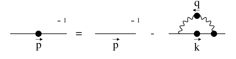
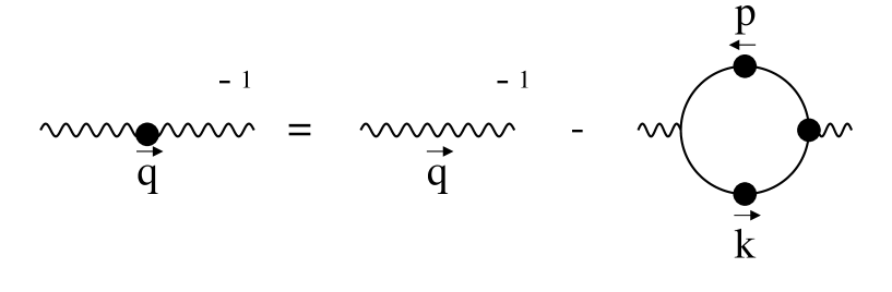
Figure 1: Schwinger-Dyson equations for the fermion and photon propagator.

Substituting $iS_{F}$ for the fermion propagator, $iD_{\mu\nu}$ for the photon propagator and $(-ie\Gamma^{\mu})$ for the vertex yields :

$$\Big{[}iS_{F}(p)\Big{]}^{-1}=\Big{[}iS_{F}^{0}(p)\Big{]}^{-1}-\frac{e^{2}}{(2\pi)^{4}}\int d^{4}k\,(i\Gamma^{\mu}(k,p))iS_{F}(k)(i\gamma^{\nu})iD_{\mu\nu}(q)\,,$$ (1)

where $q=k-p$, and

$$\Big{[}iD_{\mu\nu}(q)\Big{]}^{-1}=\Big{[}iD_{\mu\nu}^{0}(q)\Big{]}^{-1}-\frac{(-1)N_{f}e^{2}}{(2\pi)^{4}}\int d^{4}k\,\mbox{Tr}\left[(i\Gamma_{\mu}(k,p))iS_{F}(k)(i\gamma_{\nu})iS_{F}(p)\right]\,,$$ (2)

where $p=k-q$.

We define the full fermion propagator of momentum $p$ by  :

$$iS_{F}(p)=\frac{i{\cal F}(p^{2})}{/\hbox to0.0pt{\hss p}-\Sigma(p^{2})}\,.$$

The bare fermion propagator is :

$$iS_{F}^{0}(p)=\frac{i}{/\hbox to0.0pt{\hss p}-m_{0}}\,.$$

The full photon propagator of momentum $q$ is given by :

$$iD_{\mu\nu}(q)=-\frac{i}{q^{2}}\left[{\cal G}(q^{2})\left(g_{\mu\nu}-\frac{q_{\mu}q_{\nu}}{q^{2}}\right)+\xi\frac{q_{\mu}q_{\nu}}{q^{2}}\right]\,.$$ (3)

The bare photon propagator is :

$$iD_{\mu\nu}(q)=-\frac{i}{q^{2}}\left[\left(g_{\mu\nu}-\frac{q_{\mu}q_{\nu}}{q^{2}}\right)+\xi\frac{q_{\mu}q_{\nu}}{q^{2}}\right]\,.$$ (4)

From Eq. (1) one can project out the integral equations for $\Sigma(p^{2})$ and ${\cal F}(p^{2})$. In Minkowski space these are given by :

$$\frac{\Sigma(p^{2})}{{\cal F}(p^{2})} = m_{0}-\frac{ie^{2}}{4(2\pi)^{4}}\int d^{4}k\,\frac{{\cal F}(k^{2})}{(k^{2}-\Sigma^{2}(k^{2}))q^{2}}$$

$$\times\left[{\cal G}(q^{2})\left(g_{\mu\nu}-\frac{q_{\mu}q_{\nu}}{q^{2}}\right)+\xi\frac{q_{\mu}q_{\nu}}{q^{2}}\right]\mbox{Tr}[\Gamma^{\mu}(k,p)(/\hbox to0.0pt{\hss k}+\Sigma(k^{2}))\gamma^{\nu}]\,,$$

$$\frac{1}{{\cal F}(p^{2})} = 1+\frac{ie^{2}}{4(2\pi)^{4}}\frac{1}{p^{2}}\int d^{4}k\,\frac{{\cal F}(k^{2})}{(k^{2}-\Sigma^{2}(k^{2}))q^{2}}$$

$$\times\left[{\cal G}(q^{2})\left(g_{\mu\nu}-\frac{q_{\mu}q_{\nu}}{q^{2}}\right)+\xi\frac{q_{\mu}q_{\nu}}{q^{2}}\right]\mbox{Tr}[/\hbox to0.0pt{\hss p}\Gamma^{\mu}(k,p)(/\hbox to0.0pt{\hss k}+\Sigma(k^{2}))\gamma^{\nu}]\,.$$

It is important to note that unless the vertex $\Gamma^{\mu}(k,p)$ satisfies the Ward-Takahashi identity and the regularization of the loop integrals is translation invariant, the photon propagator of Eq. (2) will not have the Lorentz structure of Eq. (3) with the coefficients of $g^{\mu\nu}$ and $q^{\mu}q^{\nu}$ being related to a single function ${\cal G}(q^{2})$. When these conditions are satisfied then the integral equation for ${\cal G}(q^{2})$ can be deduced by applying the projection operator ${\cal P}_{\mu\nu}=g_{\mu\nu}-n{q_{\mu}q_{\nu}}/{q^{2}}$ (with any value of $n$) to Eq. (2) :

$$\frac{1}{{\cal G}(q^{2})} = 1-\frac{iN_{f}e^{2}}{3(2\pi)^{4}}\frac{1}{q^{2}}\int d^{4}k\,\frac{1}{(k^{2}-\Sigma^{2}(k^{2}))(p^{2}-\Sigma^{2}(p^{2}))}$$

$$\hskip 85.35826pt\times\,{\cal P}_{\mu\nu}\mbox{Tr}[\Gamma^{\mu}(k,p)(/\hbox to0.0pt{\hss k}+\Sigma(k^{2}))\gamma^{\nu}(/\hbox to0.0pt{\hss p}+\Sigma(p^{2}))]\,.$$

In general, if we regularize the theory using an ultraviolet cutoff the vacuum polarization integral in Eq. (S0.Ex5) contains a quadratic divergence which has to be removed, since such a photon mass term is not allowed in more than 2 dimensions. One can show that the $q_{\mu}q_{\nu}/q^{2}$ term of the transverse part cannot receive any quadratic divergent contribution. Consequently, if we choose the projection operator ${\cal P}_{\mu\nu}$ of Eq. (S0.Ex5) with $n=4$, the resulting integral will be free of quadratic divergences because the contraction ${\cal P}_{\mu\nu}g^{\mu\nu}$ vanishes.

A much used alternative procedure is to take the projection operator in its simplest form, ${\cal P}_{\mu\nu}=g_{\mu\nu}$. The resulting vacuum polarization integral then contains a quadratic divergence which can be removed explicitly by imposing :

$$\lim_{q^{2}\rightarrow 0}\;\frac{q^{2}}{{\cal G}(q^{2})}=0\,,$$ (8)

to ensure a massless photon. If we write the photon renormalization function as :

$${\cal G}(q^{2})=\frac{1}{1+\Pi(q^{2})}\,,$$

Eq. (8) then corresponds to a renormalization of the vacuum polarization $\Pi(q^{2})$ :

$$q^{2}\tilde{\Pi}(q^{2})=q^{2}\Pi(q^{2})-\lim_{q^{2}\rightarrow 0}q^{2}\Pi(q^{2})\,.$$ (9)

This is the procedure adopted by Kondo et al. [1]. They solve numerically the coupled set of integral equations for the dynamical fermion mass $\Sigma(p^{2})$ and the photon renormalization function ${\cal G}(q^{2})$ in the case of zero bare mass, $m_{0}\equiv 0$. The calculations are performed in the Landau gauge with the bare vertex approximation, i.e. $\Gamma^{\mu}(k,p)\equiv\gamma^{\mu}$. As a further approximation they decouple the ${\cal F}$-equation by putting ${\cal F}(p^{2})\equiv 1$. While the quadratic divergence in the vacuum polarization is removed by imposing Eq. (9), the fact that the Ward-Takahashi identity is not satisfied, when dynamical mass is generated, makes the results procedure dependent.

The integral equations one obtains using these approximations, transformed to Euclidean space, changing to spherical coordinates and introducing an ultraviolet cutoff $\Lambda^{2}$ on the radial integrals, are given by :

$$\Sigma(p^{2})=\frac{3\alpha}{2\pi^{2}}\int_{0}^{\Lambda^{2}}dk^{2}\frac{k^{2}\Sigma(k^{2})}{k^{2}+\Sigma^{2}(k^{2})}\int_{0}^{\pi}d\theta\sin^{2}\theta\frac{{\cal G}(q^{2})}{q^{2}}\,,$$ (10)

where $q^{2}=p^{2}+k^{2}-2pk\cos\theta$, with $p=\sqrt{p^{2}}$, $k=\sqrt{k^{2}}$, and

$$\frac{1}{{\cal G}(q^{2})}=1-\frac{4N_{f}\alpha}{3\pi^{2}}\frac{1}{q^{2}}\int_{0}^{\Lambda^{2}}dk^{2}\frac{k^{2}}{k^{2}+\Sigma^{2}(k^{2})}\int_{0}^{\pi}d\theta\sin^{2}\theta$$

$$\times\left\{\frac{k^{2}-kq\cos\theta+2\Sigma(k^{2})\Sigma(p^{2})}{p^{2}+\Sigma^{2}(p^{2})}-\frac{k^{2}+2\Sigma^{2}(k^{2})}{k^{2}+\Sigma^{2}(k^{2})}\right\}\,,$$

where $p^{2}=q^{2}+k^{2}-2qk\cos\theta$, with $q=\sqrt{q^{2}}$, $k=\sqrt{k^{2}}$.

The second term in $\{\cdots\}$ in Eq. (S0.Ex7) subtracts the quadratic divergence. Recall that in QED the momentum dependence of the coupling comes wholly from the photon renormalization function, so solutions for ${\cal G}(q^{2})$ give the running of the coupling. Kondo et al. solve this coupled set of non-linear integral equations, Eqs. (10, S0.Ex7), for $N_{f}=1$ and find a symmetry breaking phase for $\alpha$ greater than some critical coupling $\alpha_{c}\approx 2.084$.

In Figs. 2, 3 We display the results for a value of $\alpha=2.086$, close to its critical value. The dynamical mass function, $\Sigma(p^{2})$, is illustrated in Fig. 2. Fig. 3 shows the photon renormalization function, ${\cal G}(q^{2})$, found from their self-consistent solution and this is compared with its 1-loop approximation. One observes that at high momenta the self-consistent ${\cal G}(q^{2})$ follows the 1-loop result very nicely. For decreasing momenta the effect of the dynamically generated mass comes into play and the value of ${\cal G}(q^{2})$, and hence that of the running coupling, seems to stabilize for a while, as one could expect. Then, surprisingly, at some lower momentum there is a sudden fall in ${\cal G}(q^{2})$, which drops below the 1-loop value and almost vanishes completely. This is a rather strange behaviour for the running coupling at low momenta. This decrease corresponds to $\tilde{\Pi}(q^{2})$ of Eq. (9) becoming large.

Figure 2: Dynamical mass function $\Sigma(p^{2})$, as a function of momentum $p^{2}$ for $N_{f}=1$ and $\alpha=2.086$ as calculated in a self-consistent way as in [1] ($\Lambda=10^{5}$).

Figure 3: Photon renormalization function ${\cal G}(q^{2})$, as a function of momentum $q^{2}$ for $N_{f}=1$ and $\alpha=2.086$ as calculated in a self-consistent way as in [1] and in 1-loop approximation ($\Lambda=10^{5}$).

To solve the problem numerically Kondo et al. have made supplementary assumptions about the ultraviolet behaviour of $\Sigma(p^{2})$ and ${\cal G}(q^{2})$. These arise from the need to handle loop momenta beyond the ultraviolet (UV) cutoff. For example, if in Eq. (10) $0\leq p^{2},k^{2}\leq\Lambda^{2}$, then the photon momentum $q^{2}=p^{2}+k^{2}-2pk\cos\theta$ will lie in the interval $0\leq q^{2}\leq 4\Lambda^{2}$. The same argument holds for the fermion momentum $p^{2}$ in Eq. (S0.Ex7), i.e. $0\leq p^{2}\leq 4\Lambda^{2}$. As a consequence the angular integrals need values of $\Sigma$ and ${\cal G}$ at momenta above the UV-cutoff, this is outside the physical momentum region. Therefore one will have to extrapolate $\Sigma$ and ${\cal G}$ outside this region. In their work, Kondo et al. define :

$$\Sigma(q^{2}>\Lambda^{2}) \equiv 0$$ (12)

$$\Pi(q^{2}>\Lambda^{2}) \equiv 0\;\Rightarrow\;{\cal G}(q^{2}>\Lambda^{2})\equiv 1\,.$$ (13)

Both dynamical mass and vacuum polarization vanish above the UV-cutoff and the theory then behaves as a free theory. Although this assumption seems reasonable, Eq. (12) introduces a jump discontinuity in the dynamical mass function at $q^{2}=\Lambda^{2}$ because $\Sigma(\Lambda^{2})\neq 0$ for $\alpha>\alpha_{c}$ (see Fig. 2), while Eq. (13) introduces a relatively sharp kink in the photon renormalization function at that point (see Fig. 3).

In the physical world these functions have to be smooth. To investigate in a crude way the influence of the discontinuity in $\Sigma(p^{2})$, we can remove it by hand by defining the following simple extrapolation rule :

$$\Sigma(p^{2}>\Lambda^{2})=\Sigma(\Lambda^{2})\,\frac{\Lambda^{2}}{p^{2}}\,.$$ (14)

This will get rid of the jump discontinuity in the dynamical mass function, leaving instead a very slight kink.

When solving the integral equations using this extrapolation rule, the step in the photon renormalization function at intermediate low momenta surprisingly disappears as can be seen in Fig. 4. This was not anticipated since one would not expect the high momentum behaviour of $\Sigma(p^{2})$, where its value is quite small, to play such a major role in the behaviour of ${\cal G}(q^{2})$ at low $q^{2}$.

Figure 4: Photon renormalization function ${\cal G}(q^{2})$, as a function of momentum $q^{2}$ for $N_{f}=1$ and $\alpha=2.086$ as calculated in a self-consistent way with a continuous extrapolation for $\Sigma(p^{2})$, with the jump discontinuity in $\Sigma(p^{2})$ as in [1] and in 1-loop approximation ($\Lambda=10^{5}$).

A more detailed investigation indeed shows that the step in the photon renormalization function found by Kondo et al. is an artefact of the way they renormalize the quadratic divergence in the vacuum polarization integral, Eq. (S0.Ex7), combined with the presence of the jump discontinuity in the dynamical mass function, Eq. (12), as we now explain.

From the angular integrand of the ${\cal G}$-equation, Eq. (S0.Ex7) , we define $f_{\theta}$ as :

$$f_{\theta}=\frac{k^{2}-kq\cos\theta+2\Sigma(k^{2})\Sigma(p^{2})}{p^{2}+\Sigma^{2}(p^{2})}-\frac{k^{2}+2\Sigma^{2}(k^{2})}{k^{2}+\Sigma^{2}(k^{2})}\,.$$ (15)

Both terms in Eq. (15) cancel exactly at $q^{2}=0$ to remove the quadratic singularity. It is easy to see that provided $\Sigma(k^{2})$ is continuous for all $k^{2}$, $f_{\theta}$ will be continuous, and if $\Sigma(k^{2})$ has a Taylor series, $f_{\theta}$ will be smooth. Of course the description of the real world has to be such that the approximate cancellation of the quadratic divergence at low $q^{2}$ becomes exact at $q^{2}\ =\ 0$ in a smooth way.

Now let us look at the angular integrand $f_{\theta}$ in the approximation of Kondo et al. [1] when $q^{2}$ is small but $k^{2}$ is very large, indeed larger than $k_{0}^{2}=(\Lambda-q)^{2}$. For values of $\theta$ greater than $\theta_{0}(k^{2})=\arccos((k^{2}+q^{2}-\Lambda^{2})/2kq)$ we will have $p^{2}>\Lambda^{2}$. If we now use Kondo et al’s extrapolation, Eq. (12), then $\Sigma(p^{2}>\Lambda^{2})=0$ and the angular integrand Eq. (15), now becomes :

$$f_{\theta}=\frac{k^{2}-kq\cos\theta}{p^{2}}-\frac{k^{2}+2\Sigma^{2}(k^{2})}{k^{2}+\Sigma^{2}(k^{2})}\,.$$ (16)

When $q\rightarrow 0$, i.e. $p\rightarrow k$ :

$$f_{\theta} \approx -\frac{\Sigma^{2}(k^{2})}{k^{2}+\Sigma^{2}(k^{2})}+{\cal O}(q^{2},kq\cos\theta)\,.$$ (17)

As soon as $q^{2}$ deviates from zero, the angular integrand contains a jump discontinuity at $\theta=\theta_{0}(k^{2})$, and part of the angular integrand will not vanish continuously when $q^{2}\rightarrow 0$. In fact the angular integral $I_{\theta}$ will receive an extra contribution $\delta I_{\theta}$ when $k^{2}$ is larger than $k_{0}^{2}=(\Lambda-q)^{2}$ :

$$\delta I_{\theta}(k^{2}) = \int_{\theta_{0}(k^{2})}^{\pi}d\theta\,\sin^{2}\theta\left[-\frac{\Sigma^{2}(k^{2})}{k^{2}+\Sigma^{2}(k^{2})}\right]$$ (18)

$$= -\left(\frac{\pi}{2}-\frac{\theta_{0}(k^{2})}{2}+\frac{\sin 2\theta_{0}(k^{2})}{4}\right)\,\frac{\Sigma^{2}(k^{2})}{k^{2}+\Sigma^{2}(k^{2})}\,.$$

Substituting Eq. (18) in Eq. (S0.Ex7) we see that the vacuum polarization receives an extra contribution $\delta\Pi(q^{2})$ :

$$\delta\Pi(q^{2})=\frac{4N_{f}\alpha}{3\pi^{2}}\frac{1}{q^{2}}\int_{k_{0}^{2}}^{\Lambda^{2}}dk^{2}\,\frac{k^{2}\Sigma^{2}(k^{2})}{(k^{2}+\Sigma^{2}(k^{2}))^{2}}\left(\frac{\pi}{2}-\frac{\theta_{0}(k^{2})}{2}+\frac{\sin 2\theta_{0}(k^{2})}{4}\right)\,.$$ (19)

Writing $k=\Lambda+q\cos{\psi}$, so that $\theta_{0}\simeq\psi$ for $q^{2}<<\Lambda^{2}$, we have, using the mean value theorem :

$$\delta\Pi(q^{2})\simeq\frac{8N_{f}\alpha}{3\pi^{2}}\frac{\Lambda^{3}\Sigma^{2}(\Lambda^{2})}{q(\Lambda^{2}+\Sigma^{2}(\Lambda^{2}))^{2}}\int_{\pi/2}^{\pi}\,d\psi\sin{\psi}\left[\frac{\pi}{2}-\frac{\psi}{2}+\frac{\sin 2\psi}{4}\right]\,,$$ (20)

so that :

$$\delta\Pi(q^{2})\simeq\frac{8N_{f}\alpha}{9\pi^{2}}\frac{\Sigma^{2}(\Lambda^{2})}{q\Lambda}\,.$$ (21)

Because of the $1/q$ this change in $\Pi(q^{2})$ would be noticeable at very small values of $q^{2}$. However, this analytic calculation does not explain the sharp decrease of ${\cal G}(q^{2})$ at intermediate low momenta we and Kondo et al. [1] find — see Fig. 3.

To understand why this happens we have to consider how the numerical program computes the extra contribution Eq. (19) to the vacuum polarization integral. The integrals are approximated by a finite sum of integrand values at momenta uniformly spread on a logarithmic scale. For small $q^{2}$ the extra contribution is entirely concentrated at the uppermost momentum region of the radial integral ($k^{2}\in[k_{0}^{2},\Lambda^{2}]$). There the numerical integration program will have only one grid point situated in the interval $[k_{0}^{2},\Lambda^{2}]$ for any realistic grid distribution. This point will lie at $k^{2}=\Lambda^{2}$ if we use a closed quadrature formula. Therefore the integral will be approximated by the value of the integrand at $\Lambda^{2}$ times a weight factor $W(\Lambda^{2})=w\Lambda^{2}$ ($w$ is ${\cal O}(1)$) :

$$\delta\Pi(q^{2})\approx\frac{4N_{f}\alpha}{3\pi^{2}}\frac{W(\Lambda^{2})\Lambda^{2}\Sigma^{2}(\Lambda^{2})}{q^{2}(\Lambda^{2}+\Sigma^{2}(\Lambda^{2}))^{2}}\left(\frac{\pi}{2}-\frac{\theta_{0}(\Lambda^{2})}{2}+\frac{\sin 2\theta_{0}(\Lambda^{2})}{4}\right)\,.$$ (22)

For small $q^{2}$ we have $\theta_{0}(\Lambda^{2})\approx\pi/2$ and the extra contribution to the vacuum polarization will be :

$$\delta\Pi(q^{2})\approx\frac{N_{f}\alpha w}{3\pi}\frac{\Sigma^{2}(\Lambda^{2})}{q^{2}}\,.$$ (23)

This will effectively add a huge correction to the vacuum polarization at low $q^{2}$. This has been extensively checked numerically and shown to be completely responsible for the sudden decrease in the photon renormalization function ${\cal G}(q^{2})$ at low momenta. To reproduce our previous analytic result of Eq. (21) numerically, the integration grid has to be tuned unnaturally fine to include more points in the region $[k_{0}^{2},\Lambda^{2}]$. Without such tuning one has the result of Eq. (23). Then $q^{2}\Pi(q^{2})$ does not vanish smoothly as $q^{2}\rightarrow 0$. Instead, for $q^{2}>0$, $q^{2}\Pi(q^{2})\approx N_{f}\alpha w\Sigma^{2}(\Lambda^{2})/3\pi$ and so as soon as $q^{2}$ is non-zero the cancellation of the quadratic divergence disappears suddenly and not gradually as the physical world requires.

How can we avoid this problem? As discussed before one can introduce a smooth decrease of $\Sigma(p^{2})$ above the UV-cutoff. This ensures that the cancellation of the quadratic divergence takes place smoothly as $q^{2}\rightarrow 0$. The results obtained with the approximation of Eq. (14) are shown in Fig. 4 and are consistent with our physical intuition about the behaviour of the running of the coupling.

Once the quadratic divergence has been removed properly, other numerical difficulties start to show up. For instance, inadequate interpolation may give rise to unphysical singularities in ${\cal G}(q^{2})$. We do not discuss these further, as they are outside the scope of this note. However, we remark that these problems are avoided if one uses some smooth solution method.

We conclude that one has to ensure the proper removal of the quadratic divergence from the vacuum polarization integral when solving the coupled set of integral equations for the dynamical mass function and the photon renormalization function numerically. As shown, a very small jump discontinuity in the extrapolation of the dynamical mass function can alter the behaviour of the photon renormalization function quite dramatically at low momentum and such a peculiar running of the coupling is unphysical. To avoid this and also other numerical problems encountered in the solution of the coupled set of integral equations it would therefore be preferable to search for smooth solutions for the dynamical mass function $\Sigma(p^{2})$, the fermion wavefunction renormalization ${\cal F}(p^{2})$ and the photon renormalization function ${\cal G}(q^{2})$. A study implementing this is currently in progress. This is essential if we are to understand the phase structure of strong coupling QED in 4 dimensions in the continuum.

References

• [1] K-I.Β Kondo, H.Β Mino and H.Β Nakatani, Mod. Phys. Lett. A7 (1992) 1509.
• [2] K-I.Β Kondo and H.Β Nakatani, Nucl. Phys. B351 (1991) 236.
• [3] V.P.Β Gusynin, Mod. Phys. Lett. 5 (1990) 133.
• [4] K-I.Β Kondo and H.Β Nakatani, Prog. Theor. Phys. 88 (1992) 737.