MPI-PhT/94-96
TUM-T31-82/94
hep-ph/9501281
December 1994


Effective Hamiltonian for $B\rightarrow X_{s}e^{+}e^{-}$ Beyond Leading Logarithms in the NDR and HV Schemes

Abstract

We calculate the next-to-leading QCD corrections to the effective Hamiltonian for $B\rightarrow X_{s}e^{+}e^{-}$ in the NDR and HV schemes. We give for the first time analytic expressions for the Wilson Coefficient of the operator $Q_{9}=(\bar{s}b)_{V-A}(\bar{e}e)_{V}$ in the NDR and HV schemes. Calculating the relevant matrix elements of local operators in the spectator model we demonstrate the scheme independence of the resulting short distance contribution to the physical amplitude. Keeping consistently only leading and next-to-leading terms, we find an analytic formula for the differential dilepton invariant mass distribution in the spectator model. Numerical analysis of the $m_{\rm t}$, $\Lambda_{\overline{\rm MS}}$ and $\mu\approx{\cal O}(m_{\rm b})$ dependences of this formula is presented. We compare our results with those given in the literature.

1 Introduction

The rare decay $B\rightarrow X_{s}e^{+}e^{-}$ has been the subject of many theoretical studies in the framework of the standard model and its extensions such as the two Higgs doublet models and models involving supersymmetry [1, 2, 3, 4, 5, 6, 7, 8]. In particular the strong dependence of $B\rightarrow X_{s}e^{+}e^{-}$ on $m_{\rm t}$ has been stressed by Hou et. al. [1]. It is clear that once $B\rightarrow X_{s}e^{+}e^{-}$ has been observed, it will offer an useful test of the standard model and of its extensions. To this end the relevant branching ratio, the dilepton invariant mass distribution and other distributions of interest should be calculated with sufficient precision. In particular the QCD effects should be properly taken into account.

The central element in any analysis of $B\rightarrow X_{s}e^{+}e^{-}$ is the effective Hamiltonian for $\Delta B=1$ decays relevant for scales $\mu\approx{\cal O}(m_{\rm b})$ in which the short distance QCD effects are taken into account in the framework of a renormalization group improved perturbation theory. These short distance QCD effects have been calculated over the last years with increasing precision by several groups [2, 9, 10] culminating in a complete next-to-leading QCD calculation presented by Misiak in ref. [11] and very recently in a corrected version in [12].

The actual calculation of $B\rightarrow X_{s}e^{+}e^{-}$ involves not only the evaluation of Wilson coefficients of ten local operators (see (2.1)) which mix under renormalization but also the calculation of the corresponding matrix elements of these operators relevant for $B\rightarrow X_{s}e^{+}e^{-}$ . The latter part of the analysis can be done in the spectator model, which, according to heavy quark effective theory, for B-decays should offer a good approximation to QCD. One can also include the non-perturbative ${\cal O}(1/m_{\rm b}^{2})$ corrections to the spectator model which enhance the rate for $B\rightarrow X_{s}e^{+}e^{-}$ by roughly 10% [13]. A realistic phenomenological analysis should also include the long distance contributions which are mainly due to the $J/\psi$ and $\psi^{\prime}$ resonances [14, 15, 16]. Since in this paper we are mainly interested in the next-to-leading short distance QCD corrections to the spectator model we will not include these complications in what follows.

It is well known that the Wilson coefficients of local operators depend beyond the leading logarithmic approximation on the renormalization scheme for operators, in particular on the treatment of $\gamma_{5}$ in $D\not=4$ dimensions. This dependence must be cancelled by the scheme dependence present in the matrix elements of operators so that the final decay amplitude does not depend on the renormalization scheme. In the context of $B\rightarrow X_{s}e^{+}e^{-}$ this point has been emphasized in particular by Grinstein et. al. [2]. Other examples such as $K\rightarrow\pi\pi$, $K_{L,S}\rightarrow\pi^{0}e^{+}e^{-}$, $B\rightarrow X_{s}\gamma$ can be found in refs. [17, 18, 19]. The interesting feature of $B\rightarrow X_{s}e^{+}e^{-}$ as compared to decays such as $K\rightarrow\pi\pi$, is the fact that due to the ability of calculating reliably the matrix elements of all operators contributing to this decay, the cancellation of scheme dependence can be demonstrated in the actual calculation of the short distance part of the physical amplitude.

Now all the existing calculations of $B\rightarrow X_{s}e^{+}e^{-}$ use the NDR renormalization scheme (anticommuting $\gamma_{5}$ in $D\not=4$ dimensions). Even if arguments have been given, in particular in [2] and [11], how the cancellation of the scheme dependence in $B\rightarrow X_{s}e^{+}e^{-}$ would take place, it is of interest to see this explicitly by calculating this decay in two different renormalization schemes. In addition, in view of the complexity of next-to-leading order (NLO) calculations and the fact that the only complete NLO analysis of $B\rightarrow X_{s}e^{+}e^{-}$ has been done by a single person, it is important to check the results of refs. [11, 12].

Here we will present the calculations of the Wilson coefficients and matrix elements relevant for $B\rightarrow X_{s}e^{+}e^{-}$ in two renormalization schemes (NDR and HV [20]) demonstrating the scheme independence of the resulting amplitude. Beside this the main results of our paper are as follows:

• We give for the first time analytic NLO expressions for the Wilson coefficient of the operator $Q_{9}=(\bar{s}b)_{V-A}(\bar{e}e)_{V}$ in the NDR and HV schemes.

• Calculating the matrix elements of local operators in the spectator model we fully agree with Misiak’s result for the dilepton invariant mass distribution very recently given in [12].

• We find, that in the HV scheme the scheme dependent term in the matrix elements (the so called $\xi$-term) receives in addition to current-current contributions also contributions from QCD penguin operators which are necessary for the cancellation of the scheme dependence in the final amplitude. This should be compared with the discussion of the scheme dependence given in refs. [2] and [11] where the $\xi$-term received only contributions from current-current operators.

• We stress that in a consistent NLO analysis of the decay $B\rightarrow X_{s}e^{+}e^{-}$ , one should on one hand calculate the Wilson coefficient of the operator $Q_{9}=(\bar{s}b)_{V-A}(\bar{e}e)_{V}$ including leading and next-to-leading logarithms, but on the other hand only leading logarithms should be kept in the remaining Wilson coefficients. Only then a scheme independent amplitude can be obtained. This special treatment of $Q_{9}$ is related to the fact that strictly speaking in the leading logarithmic approximation only this operator contributes to $B\rightarrow X_{s}e^{+}e^{-}$ . The contributions of the usual current-current operators, QCD penguin operators, magnetic penguin operators and of $Q_{10}=(\bar{s}b)_{V-A}(\bar{e}e)_{A}$ enter only at the NLO level and to be consistent only the leading contributions to the corresponding Wilson coefficients should be included. In this respect we differ from the original analysis of Misiak [11] who in his numerical evaluation of $B\rightarrow X_{s}e^{+}e^{-}$ also included partially known NLO corrections to Wilson coefficients of operators $Q_{i}(i\not=9)$. These additional corrections are, however, scheme dependent and are really a part of still higher order in the renormalization group improved perturbation theory. The most recent analysis of Misiak [12] does not include these contributions and can be directly compared with the present paper.

• Keeping consistently only the leading and next-to-leading contributions to $B\rightarrow X_{s}e^{+}e^{-}$ we are able to give analytic expressions for all Wilson coefficients which should be useful for phenomenological applications.

Our paper is organized as follows:

In sect. 2 we collect the master formulae for $B\rightarrow X_{s}e^{+}e^{-}$ in the spectator model which include consistently leading and next-to-leading logrithms. In sect. 3 we describe some details of the NLO calculation of the Wilson coefficient $C_{9}(\mu)$ and of the relevant one-loop matrix elements in NDR and HV schemes. In sect. 4 we present a numerical analysis. We end our paper with a brief summary of the main results.

2 Master Formulae

2.1 Operators

Our basis of operators is given as follows:

$$\begin{array}[]{rcl}Q_{1}&=&(\bar{s}_{\alpha}c_{\beta})_{V-A}(\bar{c}_{\beta}b_{\alpha})_{V-A}\vspace{0.2cm}\\ Q_{2}&=&(\bar{s}c)_{V-A}(\bar{c}b)_{V-A}\vspace{0.2cm}\\ Q_{3}&=&(\bar{s}b)_{V-A}\sum_{q}(\bar{q}q)_{V-A}\vspace{0.2cm}\\ Q_{4}&=&(\bar{s}_{\alpha}b_{\beta})_{V-A}\sum_{q}(\bar{q}_{\beta}q_{\alpha})_{V-A}\vspace{0.2cm}\\ Q_{5}&=&(\bar{s}b)_{V-A}\sum_{q}(\bar{q}q)_{V+A}\vspace{0.2cm}\\ Q_{6}&=&(\bar{s}_{\alpha}b_{\beta})_{V-A}\sum_{q}(\bar{q}_{\beta}q_{\alpha})_{V+A}\vspace{0.2cm}\\ Q_{7}&=&\frac{e}{8\pi^{2}}m_{b}\bar{s}_{\alpha}\sigma^{\mu\nu}(1+\gamma_{5})b_{\alpha}F_{\mu\nu}\vspace{0.2cm}\\ Q_{8}&=&\frac{g}{8\pi^{2}}m_{b}\bar{s}_{\alpha}\sigma^{\mu\nu}(1+\gamma_{5})T^{a}_{\alpha\beta}b_{\beta}G^{a}_{\mu\nu}\vspace{0.2cm}\\ Q_{9}&=&(\bar{s}b)_{V-A}(\bar{e}e)_{V}\vspace{0.2cm}\\ Q_{10}&=&(\bar{s}b)_{V-A}(\bar{e}e)_{A}\end{array}$$ (2.1)

where $\alpha$ and $\beta$ denote colour indices. We omit the colour indices for the colour-singlet currents. Labels $(V\pm A)$ refer to $\gamma_{\mu}(1\pm\gamma_{5})$. $Q_{1,2}$ are the current-current operators, $Q_{3-6}$ the QCD penguin operators, $Q_{7,8}$ “magnetic penguin” operators and $Q_{9,10}$ semi-leptonic electroweak penguin operators. Our normalizations are as in refs. [18] and [19].

2.2 Wilson Coefficients

The Wilson coefficients for the operators $Q_{1}$–$Q_{7}$ are given in the leading logarithmic approximation by [18, 21, 22, 23]

$$C_{j}^{(0)}(\mu) = \sum_{i=1}^{8}k_{ji}\eta^{a_{i}}\qquad(j=1,...6)\vspace{0.2cm}$$ (2.2)

$$C_{7}^{(0)eff}(\mu) = \eta^{\frac{16}{23}}C_{7}^{(0)}(M_{\rm W})+\frac{8}{3}\left(\eta^{\frac{14}{23}}-\eta^{\frac{16}{23}}\right)C_{8}^{(0)}(M_{\rm W})+\sum_{i=1}^{8}h_{i}\eta^{a_{i}},$$ (2.3)

with

$$\eta = \frac{\alpha_{s}(M_{\rm W})}{\alpha_{s}(\mu)},$$ (2.4)

$$C_{7}^{(0)}(M_{\rm W}) = -\frac{1}{2}A(x_{t}),$$ (2.5)

$$C_{8}^{(0)}(M_{\rm W}) = -\frac{1}{2}F(x_{t}),$$ (2.6)

where $x_{t}=m_{\rm t}^{2}/M_{\rm W}^{2}$ and $A(x)$ and $F(x)$ are defined in (2.14) and (2.19). The numbers $a_{i}$, $k_{ji}$ and $h_{i}$ are given by

$$\begin{array}[]{rrrrrrrrrl}a_{i}=(\!\!&\frac{14}{23},&\frac{16}{23},&\frac{6}{23},&-\frac{12}{23},&0.4086,&-0.4230,&-0.8994,&0.1456&\!\!)\vspace{0.1cm}\\ k_{1i}=(\!\!&0,&0,&\frac{1}{2},&-\frac{1}{2},&0,&0,&0,&0&\!\!)\vspace{0.1cm}\\ k_{2i}=(\!\!&0,&0,&\frac{1}{2},&\frac{1}{2},&0,&0,&0,&0&\!\!)\vspace{0.1cm}\\ k_{3i}=(\!\!&0,&0,&-\frac{1}{14},&\frac{1}{6},&0.0510,&-0.1403,&-0.0113,&0.0054&\!\!)\vspace{0.1cm}\\ k_{4i}=(\!\!&0,&0,&-\frac{1}{14},&-\frac{1}{6},&0.0984,&0.1214,&0.0156,&0.0026&\!\!)\vspace{0.1cm}\\ k_{5i}=(\!\!&0,&0,&0,&0,&-0.0397,&0.0117,&-0.0025,&0.0304&\!\!)\vspace{0.1cm}\\ k_{6i}=(\!\!&0,&0,&0,&0,&0.0335,&0.0239,&-0.0462,&-0.0112&\!\!)\vspace{0.1cm}\\ h_{i}=(\!\!&2.2996,&-1.0880,&-\frac{3}{7},&-\frac{1}{14},&-0.6494,&-0.0380,&-0.0186,&-0.0057&\!\!).\end{array}$$ (2.7)

The first correct calculation of the two-loop anomalous dimensions relevant for (2.3) has been presented in [21, 22] and confirmed subsequently in [24, 25, 12].

The coefficient $C_{8}^{(0)eff}(\mu)$ does not enter the formula for $B\rightarrow X_{s}e^{+}e^{-}$ at this level of accuracy. An analytic formula is given in ref. [18].

The coefficient of $Q_{10}$ is given by

$$C_{10}(M_{\rm W})=\frac{\alpha}{2\pi}\widetilde{C}_{10}(M_{\rm W}),\hskip 28.45274pt\widetilde{C}_{10}(M_{\rm W})=-\frac{Y(x_{t})}{\sin^{2}\Theta_{W}}$$ (2.8)

with $Y(x)$ given in (2.13). Since $Q_{10}$ does not renormalize under QCD, its coefficient does not depend on $\mu\approx{\cal O}(m_{\rm b})$. The only renormalization scale dependence in (2.8) enters through the definition of the top quark mass. We will return to this issue in sect. 4.

Finally, including leading as well as next-to-leading logarithms, we find

$$C_{9}^{NDR}(\mu) = \frac{\alpha}{2\pi}\widetilde{C}_{9}^{NDR}(\mu)$$ (2.9)

$$\widetilde{C}_{9}^{NDR}(\mu) = P_{0}^{NDR}+\frac{Y(x_{t})}{\sin^{2}\Theta_{W}}-4Z(x_{t})+P_{E}E(x_{t})$$ (2.10)

with

$$P_{0}^{NDR} = \frac{\pi}{\alpha_{s}(M_{W})}(-0.1875+\sum_{i=1}^{8}p_{i}\eta^{a_{i}+1})$$ (2.11)

$$+1.2468+\sum_{i=1}^{8}\eta^{a_{i}}[r^{NDR}_{i}+s_{i}\eta]$$

$$P_{E} = 0.1405+\sum_{i=1}^{8}q_{i}\eta^{a_{i}+1}$$ (2.12)

$$Y(x) = C(x)-B(x),\hskip 28.45274ptZ(x)=C(x)+\frac{1}{4}D(x).$$ (2.13)

Here

$$A(x) = \frac{x(8x^{2}+5x-7)}{12(x-1)^{3}}+\frac{x^{2}(2-3x)}{2(x-1)^{4}}\ln x,$$ (2.14)

$$B(x) = \frac{x}{4(1-x)}+\frac{x}{4(x-1)^{2}}\ln x,$$ (2.15)

$$C(x) = \frac{x(x-6)}{8(x-1)}+\frac{x(3x+2)}{8(x-1)^{2}}\ln x,$$ (2.16)

$$D(x) = \frac{-19x^{3}+25x^{2}}{36(x-1)^{3}}+\frac{x^{2}(5x^{2}-2x-6)}{18(x-1)^{4}}\ln x-\frac{4}{9}\ln x,$$ (2.17)

$$E(x) = \frac{x(18-11x-x^{2})}{12(1-x)^{3}}+\frac{x^{2}(15-16x+4x^{2})}{6(1-x)^{4}}\ln x-\frac{2}{3}\ln x,$$ (2.18)

$$F(x) = \frac{x(x^{2}-5x-2)}{4(x-1)^{3}}+\frac{3x^{2}}{2(x-1)^{4}}\ln x.$$ (2.19)

The coefficients $p_{i}$, $r^{NDR}_{i}$, $s_{i}$, and $q_{i}$ are found to be as follows:

$$\begin{array}[]{rrrrrrrrrl}p_{i}=(\!\!&0,&0,&-\frac{80}{203},&\frac{8}{33},&0.0433,&0.1384,&0.1648&-0.0073&\!\!)\vspace{0.1cm}\\ r^{NDR}_{i}=(\!\!&0,&0,&0.8966,&-0.1960,&-0.2011,&0.1328,&-0.0292,&-0.1858&\!\!)\vspace{0.1cm}\\ s_{i}=(\!\!&0,&0,&-0.2009,&-0.3579,&0.0490,&-0.3616,&-0.3554,&0.0072&\!\!)\vspace{0.1cm}\\ q_{i}=(\!\!&0,&0,&0,&0,&0.0318,&0.0918,&-0.2700,&0.0059&\!\!).\end{array}$$ (2.20)

$P_{E}$ is ${\cal O}(10^{-2})$ and consequently the last term in (2.10) can be neglected. We keep it however in our numerical analysis.

In the HV scheme only the coefficients $r_{i}$ are changed. They are given by

$$\begin{array}[]{lrrrrrrrrl}r^{HV}_{i}=(\!\!&0,&0,&-0.1193,&0.1003,&-0.0473,&0.2323,&-0.0133,&-0.1799&\!\!).\end{array}$$ (2.21)

Equivalently we can write

$$P_{0}^{HV}=P_{0}^{NDR}+\xi^{HV}\frac{4}{9}\left(3C_{1}^{(0)}+C_{2}^{(0)}-C_{3}^{(0)}-3C_{4}^{(0)}\right)$$ (2.22)

with

$$\xi=\left\{\begin{array}[]{rl}0,&\mbox{NDR}\\ -1,&\mbox{HV.}\end{array}\right.$$ (2.23)

We note that

$$\sum_{i=1}^{8}p_{i}=0.1875,\hskip 125.19194pt\sum_{i=1}^{8}q_{i}=-0.1405,$$ (2.24)

$$\sum_{i=1}^{8}(r_{i}+s_{i})=-1.2468+\frac{4}{9}(1+\xi),\hskip 28.45274pt\sum_{i=1}^{8}p_{i}(a_{i}+1)=-\frac{16}{69}.$$ (2.25)

In this way for $\eta=1$ we find $P_{E}=0$, $P_{0}^{NDR}=4/9$ and $P_{0}^{HV}=0$ in accordance with the initial conditions in (3.3). Moreover, the second relation in (2.25) assures the correct large logarithm in $P_{0}^{NDR}$, i. e.  $8/9\,\ln(M_{\rm W}/\mu)$. The derivation of (2.9)–(2.22) is given in sect. 3.

2.3 The Differential Decay Rate

Introducing

$$\hat{s}=\frac{(p_{e^{+}}+p_{e^{-}})^{2}}{m_{\rm b}^{2}},\hskip 28.45274ptz=\frac{m_{\rm c}}{m_{\rm b}}$$ (2.26)

and calculating the one-loop matrix elements of $Q_{i}$ using the spectator model in the NDR scheme we find

$$R(\hat{s})\equiv\frac{\frac{d}{d\hat{s}}\Gamma(\mbox{$b\rightarrow se^{+}e^{-}$ })}{\Gamma(\mbox{$b\rightarrow ce\bar{\nu}$ })} = \frac{\alpha^{2}}{4\pi^{2}}\left|\frac{V_{ts}}{V_{cb}}\right|^{2}\frac{(1-\hat{s})^{2}}{f(z)\kappa(z)}\cdot\biggl{[}(1+2\hat{s})\left(|\widetilde{C}_{9}^{eff}|^{2}+|\widetilde{C}_{10}|^{2}\right)+$$ (2.27)

$$4\left(1+\frac{2}{\hat{s}}\right)|C_{7}^{(0)eff}|^{2}+12C_{7}^{(0)eff}\ {\rm Re}\,\widetilde{C}_{9}^{eff}\biggr{]}$$

where

$$\widetilde{C}_{9}^{eff} = \widetilde{C}_{9}^{NDR}\tilde{\eta}(\hat{s})+h(z,\hat{s})\left(3C_{1}^{(0)}+C_{2}^{(0)}+3C_{3}^{(0)}+C_{4}^{(0)}+3C_{5}^{(0)}+C_{6}^{(0)}\right)$$ (2.28)

$$-\frac{1}{2}h(1,\hat{s})\left(4C_{3}^{(0)}+4C_{4}^{(0)}+3C_{5}^{(0)}+C_{6}^{(0)}\right)$$

$$-\frac{1}{2}h(0,\hat{s})\left(C_{3}^{(0)}+3C_{4}^{(0)}\right)+\frac{2}{9}\left(3C_{3}^{(0)}+C_{4}^{(0)}+3C_{5}^{(0)}+C_{6}^{(0)}\right).$$

Here

$$h(z,\hat{s}) = -\frac{8}{9}\ln\frac{m_{b}}{\mu}-\frac{8}{9}\ln z+\frac{8}{27}+\frac{4}{9}x$$ (2.31)

$$-\frac{2}{9}(2+x)|1-x|^{1/2}\left\{\begin{array}[]{ll}\left(\ln\left|\frac{\sqrt{1-x}+1}{\sqrt{1-x}-1}\right|-i\pi\right),&\mbox{for }x\equiv\frac{4z^{2}}{\hat{s}}<1\\ 2\arctan\frac{1}{\sqrt{x-1}},&\mbox{for }x\equiv\frac{4z^{2}}{\hat{s}}>1,\end{array}\right.$$

$$h(0,\hat{s}) = \frac{8}{27}-\frac{8}{9}\ln\frac{m_{\rm b}}{\mu}-\frac{4}{9}\ln\hat{s}+\frac{4}{9}i\pi.$$ (2.32)

$$f(z) = 1-8z^{2}+8z^{6}-z^{8}-24z^{4}\ln z,$$ (2.33)

$$\kappa(z) = 1-\frac{2\alpha_{s}(\mu)}{3\pi}\left[(\pi^{2}-\frac{31}{4})(1-z)^{2}+\frac{3}{2}\right]$$ (2.34)

$$\tilde{\eta}(\hat{s}) = 1+\frac{\alpha_{s}(\mu)}{\pi}\,\omega(\hat{s})$$ (2.35)

with

$$\omega(\hat{s}) = -\frac{2}{9}\pi^{2}-\frac{4}{3}\mbox{Li}_{2}(s)-\frac{2}{3}\ln s\ln(1-s)-\frac{5+4s}{3(1+2s)}\ln(1-s)-$$ (2.36)

$$\frac{2s(1+s)(1-2s)}{3(1-s)^{2}(1+2s)}\ln s+\frac{5+9s-6s^{2}}{6(1-s)(1+2s)}.$$

Here $f(z)$ and $\kappa(z)$ are the phase-space factor and the single gluon QCD correction to the $b\rightarrow ce\bar{\nu}$ decay [26, 27] respectively. $\tilde{\eta}$ on the other hand represents single gluon corrections to the matrix element of $Q_{9}$ with $m_{\rm s}=0$ [28, 12]. For consistency reasons this correction should only multiply the leading logarithmic term in $P_{0}^{NDR}$.

In the HV scheme the one-loop matrix elements are different and one finds an additional explicit contribution to (2.28) given by

$$-\xi^{HV}\frac{4}{9}\left(3C_{1}^{(0)}+C_{2}^{(0)}-C_{3}^{(0)}-3C_{4}^{(0)}\right).$$ (2.37)

However $\widetilde{C}_{9}^{NDR}$ has to be replaced by $\widetilde{C}_{9}^{HV}$ given in (2.10) and (2.22) and consequently $\widetilde{C}_{9}^{eff}$ is the same in both schemes.

The first term in the function $h(z,\hat{s})$ in (2.31) represents the leading $\mu$-dependence in the matrix elements. It is cancelled by the $\mu$-dependence present in the leading logarithm in $\widetilde{C}_{9}$. The $\mu$-dependence present in the coefficients of the other operators can only be cancelled by going to still higher order in the renormalization group improved perturbation theory. To this end the matrix elements of four-quark operators should be evaluated at two-loop level. Also certain unknown three-loop anomalous dimensions should be included in the evaluation of $C_{7}^{eff}$ and $C_{9}$ [18, 19]. Certainly this is beyond the scope of the present paper and we will only investigate the left-over $\mu$-dependence in sect. 4.

The fact that the coefficient $C_{9}$ should include next-to-leading logarithms and the other coefficients should be calculated in the leading logarithmic approximation is easy to understand. There is a large logarithm in $C_{9}$ represented by $1/\alpha_{s}$ in $P_{0}$ in (2.11). Consequently the renormalization group improved perturbation theory for $C_{9}$ has the structure ${\cal O}(1/\alpha_{s})+{\cal O}(1)+{\cal O}(\alpha_{s})+\ldots$ whereas the corresponding series for the remaining coefficients is ${\cal O}(1)+{\cal O}(\alpha_{s})+\ldots$. Therefore in order to find the next-to-leading ${\cal O}(1)$ term, the full two-loop renormalization group analysis for the operators in (2.1) has to be performed in order to find $C_{9}$, but the coefficients of the remaining operators should be taken in the leading logarithmic approximation. This is gratifying because the coefficient of the magnetic operator $Q_{7}$ is known only in the leading logarithmic approximation. $Q_{7}$ does not mix with $Q_{9}$ and has no impact on the coefficients $C_{1}$–$C_{6}$. Consequently the necessary two-loop renormalization group analysis of $C_{9}$ can be performed independently of the presence of the magnetic operators, which was also the case of the decay $K_{L}\rightarrow\pi^{0}e^{+}e^{-}$ presented in ref. [19].

Let us finally compare our main formulae (2.27)–(2.37) with the ones given in the literature:

1. The general expression (2.27) with $\kappa(z)=1$ is due to Grinstein et. al. [2] who in their approximate leading order renormalization group analysis kept only the operators $Q_{1},Q_{2},Q_{7},Q_{9},Q_{10}$.

2. Inserting $C_{i}^{(0)}$ and $\widetilde{C}_{9}^{NDR}$ in (2.2)and (2.8) into (2.28) we find an analytic expression for $\widetilde{C}_{9}^{eff}$ which agrees with a recent independent calculation of Misiak [12].

3. The sign of $i\pi$ in (2.31) differs from the one given in [2] and [11] but agrees with [12] and also with the work of Fleischer [29].

4. The “$\xi$-term” given in (2.37) contains in the HV scheme also contributions from the operators $Q_{3}$ and $Q_{4}$, which are however negligible. The discussion of the “$\xi$-term” in refs. [2] and [11] does not apply then to the HV scheme.

3 Technical Details

3.1 Wilson Coefficients

In order to calculate the coefficient $C_{9}$ including next-to-leading order corrections we have to perform in principle a two-loop renormalization group analysis for the full set of operators given in (2.1). However, $Q_{10}$ is not renormalized and the dimension five operators $Q_{7}$ and $Q_{8}$ have no impact on $C_{9}$. Consequently only a set of seven operators, $Q_{1-6}$ and $Q_{9}$, has to be considered. This is precisely the case of the decay $K_{L}\rightarrow\pi^{0}e^{+}e^{-}$ considered in [19] except for an appropriate change of quark flavours and the fact that now $\mu\approx{\cal O}(m_{\rm b})$ instead of $\mu\approx{\cal O}(1\,{\rm GeV})$ should be considered. Because our detailed NLO analysis of $K_{L}\rightarrow\pi^{0}e^{+}e^{-}$ has already been published we will only discuss very briefly an analogous calculation of $B\rightarrow X_{s}e^{+}e^{-}$ , referring the interested reader to [19]. We should stress that Misiak [11, 12] used different conventions for the evanescent operators than used in [19] and here. The agreement on $\widetilde{C}_{9}^{eff}$ is therefore particularly satisfying.

Integrating out simultaneously $W,Z$ and $t$ we construct first the effective Hamiltonian for $\Delta B=1$ transitions relevant for $b\rightarrow se^{+}e^{-}$ with the operators normalized at $\mu=M_{\rm W}$. Dropping the operators $Q_{7}$, $Q_{8}$ and $Q_{10}$ for the reasons stated above and using the unitarity of the CKM matrix we find

$${\cal H}_{eff}(\Delta B=1) = -\frac{G_{F}}{\sqrt{2}}V_{ts}^{*}V_{tb}\left[\sum_{i=1}^{6}C_{i}(M_{\rm W})Q_{i}+C^{\prime}_{9}(M_{\rm W})Q^{\prime}_{9}\right]$$ (3.1)

$$+\frac{G_{F}}{\sqrt{2}}V_{us}^{*}V_{ub}\left[C_{1}(M_{\rm W})(Q_{1}^{(u)}-Q_{1})+C_{2}(M_{\rm W})(Q_{2}^{(u)}-Q_{2})\right].$$

Here $Q_{1,2}^{(u)}$ are obtained from $Q_{1,2}$ through the replacement $c\rightarrow u$. In order to make all the elements of the anomalous dimension matrix be of the same order in $\alpha_{s}$, we have appropriately rescaled $C_{9}$ and $Q_{9}$:

$$Q^{\prime}_{9}=\frac{\alpha}{\alpha_{s}(\mu)}Q_{9},\hskip 28.45274ptC^{\prime}_{9}(\mu)=\frac{\alpha_{s}(\mu)}{\alpha}C_{9}(\mu)$$ (3.2)

Note that because of GIM cancellation there are no penguin contributions in the term proportional to $V_{us}^{*}V_{ub}$. They would appear only at scales $\mu<m_{\rm c}$ as was the case in $K_{L}\rightarrow\pi^{0}e^{+}e^{-}$ . Since $|V_{us}^{*}V_{ub}/V_{ts}^{*}V_{tb}|<0.02$ we will drop the second term in what follows.

The initial conditions at $\mu=M_{\rm W}$ for the coefficients $C_{1}$–$C_{6}$ in NDR and HV schemes have been given in sect. 2.4 and in the appendix A of ref. [19] respectively. Here it suffices to give only the initial condition for the coefficient $C^{\prime}_{9}$ (denoted by $C^{\prime}_{7V}$ in [19]) which reads:

$$C^{\prime}_{9}(M_{\rm W})=\frac{\alpha_{s}(M_{\rm W})}{2\pi}\left[\frac{Y(x_{t})}{\sin^{2}\Theta_{W}}-4Z(x_{t})+\frac{4}{9}(1+\xi)\right],$$ (3.3)

where $\xi$ has been defined in (2.23). The $x_{t}$ dependence originates in box diagrams and in the $\gamma$- and $Z$-penguin diagrams [30].

With

$$\vec{C}^{T}\equiv\left(C_{1},\ldots,C_{6},C^{\prime}_{9}\right)$$ (3.4)

one can calculate the coefficients $C_{i}(\mu)$ by using the evolution operator $\hat{U}_{5}(\mu,M_{\rm W})$ relevant for an effective theory with $f=5$ flavours:

$$\vec{C}(\mu)=\hat{U}_{5}(\mu,M_{\rm W})\vec{C}(M_{\rm W}).$$ (3.5)

An explicit expression for $\hat{U}_{5}$ is given in sect. 2 of [19] where also the relevant expressions for one- and two-loop anomalous dimensions can be found. One only has to set $f=5$, $u=2$ and $d=3$ in the formulae given in [19].

Using (3.5) and rescaling back the operator $Q_{9}$ we find at $\mu\approx{\cal O}(m_{\rm b})$

$${\cal H}_{eff}(\Delta B=1)=-\frac{G_{F}}{\sqrt{2}}V_{ts}^{*}V_{tb}\left[\sum_{i=1}^{6}C_{i}(\mu)Q_{i}+C_{9}(\mu)Q_{9}\right]$$ (3.6)

with the coefficient $C_{9}(\mu)$ given in (2.10) and (2.22) for NDR and HV schemes respectively. The result for HV can either be found directly using (3.5) or by using the relation

$$\vec{C}^{HV}(\mu)=\left(\hat{1}-\frac{\alpha_{s}(\mu)}{4\pi}\Delta\hat{r}^{T}\right)\vec{C}^{NDR}(\mu)$$ (3.7)

with the matrix $\Delta\hat{r}$ given in appendix A of ref.[19].

3.2 One-Loop Matrix Elements

The operators $Q_{7}$ and $Q_{10}$ contribute at this level of accuracy only through tree level matrix elements. $Q_{8}$ contributes only through the renormalization of $Q_{7}$ and its impact is only felt in $C_{7}^{(0)eff}$. The four-quark operators $Q_{1-6}$, contribute at one-loop level through the diagrams in fig. 1 where “$\otimes\,\otimes$” denotes the operator insertion. Finally at next-to-leading level ${\cal O}(\alpha_{s})$ corrections to the matrix element $\langle Q_{9}\rangle$ have to be calculated.

Figure 1: The two possibilites for insertion of a four-quark operator into a penguin diagram.

Let us begin with $\langle Q_{1-6}\rangle$. As usual two types of insertions of the operators into the penguin diagrams have to be considered. As already discussed in ref. [31] the appearance of a closed fermion loop in fig. 1a does not pose any problems in the NDR scheme because nowhere in the calculation one has to evaluate Tr$[\gamma_{\mu}\gamma_{\nu}\gamma_{\rho}\gamma_{\lambda}\gamma_{5}]$. The diagrams in fig. 1 have been evaluated for the operators $Q_{1}$ and $Q_{2}$ by Grinstein et. al. [2] and by Misiak [11] for the full set $Q_{1}$–$Q_{6}$. These calculations have been done in the NDR scheme. Calculating these diagrams in the NDR and HV schemes we find

$$\langle Q_{1}\rangle = \frac{\alpha}{2\pi}\left(3h(z,\hat{s})-\frac{4}{3}\xi\right)\langle Q_{9}\rangle_{0}$$

$$\langle Q_{2}\rangle = \frac{\alpha}{2\pi}\left(h(z,\hat{s})-\frac{4}{9}\xi\right)\langle Q_{9}\rangle_{0}$$

$$\langle Q_{3}\rangle = \frac{\alpha}{2\pi}\left(3h(z,\hat{s})-2h(1,\hat{s})-\frac{1}{2}h(0,\hat{s})+\frac{2}{3}+\frac{4}{9}\xi\right)\langle Q_{9}\rangle_{0}$$ (3.8)

$$\langle Q_{4}\rangle = \frac{\alpha}{2\pi}\left(h(z,\hat{s})-2h(1,\hat{s})-\frac{3}{2}h(0,\hat{s})+\frac{2}{9}+\frac{4}{3}\xi\right)\langle Q_{9}\rangle_{0}$$

$$\langle Q_{5}\rangle = \frac{\alpha}{2\pi}\left(3h(z,\hat{s})-\frac{3}{2}h(1,\hat{s})+\frac{2}{3}\right)\langle Q_{9}\rangle_{0}$$

$$\langle Q_{6}\rangle = \frac{\alpha}{2\pi}\left(h(z,\hat{s})-\frac{1}{2}h(1,\hat{s})+\frac{2}{9}\right)\langle Q_{9}\rangle_{0}$$

with $\xi$ defined in (2.23), $\langle Q_{9}\rangle_{0}$ denoting the tree level matrix element of $Q_{9}$ and

$$h(z,\hat{s})=\frac{2}{3}G(z,\hat{s})-\frac{4}{9}-\frac{8}{9}\ln\frac{m_{\rm b}}{\mu}.$$ (3.9)

Here

$$G(z,\hat{s})=-4\int\limits_{0}^{1}\!\!dx\,x(1-x)\ln\left(z^{2}-\hat{s}x(1-x)\right)$$ (3.10)

with $z$ and $\hat{s}$ defined in (2.26).

A few remarks should be made:

• $h(z,\hat{s})$, $h(1,\hat{s})$ and $h(0,\hat{s})$ correspond to internal $c$, $b$ and massless $(u,d,s)$ quarks in fig. 1 respectively.

• The contributions of $(u,d,s)$ to diagram 1a) cancel each other and consequently $h(0,\hat{s})$ represents the contribution of the internal strange quark in diagram 1b).

• We note that $\langle Q_{5}\rangle$ and $\langle Q_{6}\rangle$ matrix elements do not contain the $\xi$-term. We should however stress that generally it is certainly possible to find schemes in which $\langle Q_{5}\rangle$ and $\langle Q_{6}\rangle$ matrix elements can differ from the ones given in (3.2). Similarly we have no argument that in schemes different from NDR and HV the matrix elements are found simply by changing the value of $\xi$ in the formulae given above. It could be that the changes are more involved. Consequently the discussions of the $\xi$-term presented in [2] and [11] are not generally valid.

The one gluon correction to the matrix element of $Q_{9}$, $\tilde{\eta}(\hat{s})$, can be inferred from [28] as has been noticed by Misiak in [12]. In [28] a left-handed current has been considered. Thus we rewrite the vector current as a sum of left- and right-handed currents. Neglecting the electron masses these two contributions do not interfere. Charge conjugation transforms the right-handed current into a left-handed one. Since $\hat{s}$ is invariant under this transformation both currents lead to the same invariant mass spectrum. Therefore we can write

$$\omega(\hat{s})=\frac{-2}{(1-\hat{s})^{2}(1+2\hat{s})}\int\limits_{\hat{s}}^{1}\!\!dx\tilde{F}_{1}(x,\hat{s})$$ (3.11)

with $\tilde{F}_{1}(x,\hat{s})$ defined explicitly in eq. (3.9) of [28]. Calculating the integral we arrive at the result given in (2.36) which furthermore agrees with Misiak [32].

4 Numerical Analysis

In our numerical analysis we will use

$$\alpha_{s}(\mu)=\frac{4\pi}{\beta_{0}\ln(\mu^{2}/\Lambda_{\overline{\rm MS}}^{2})}\left[1-\frac{\beta_{1}}{\beta_{0}^{2}}\frac{\ln\ln(\mu^{2}/\Lambda_{\overline{\rm MS}}^{2})}{\ln(\mu^{2}/\Lambda_{\overline{\rm MS}}^{2})}\right]$$ (4.12)

with $\beta_{0}=23/3$ and $\beta_{1}=116/3$ as appropriate for five flavours. We also take $\Lambda_{\overline{\rm MS}}=(225\pm 85)\,{\rm MeV}$ corresponding to $\alpha_{s}(M_{\rm Z})=0.117\pm 0.007$. For the remaining parameters we take

$$\begin{array}[]{rclrcl}\alpha&=&1/129,&m_{\rm c}&=&1.4\,{\rm GeV},\\ \sin^{2}\theta_{W}&=&0.23,&m_{\rm b}&=&4.8\,{\rm GeV},\\ |V_{ts}/V_{cb}|&=&1,&M_{\rm W}&=&80.0\,{\rm GeV}.\end{array}$$

In table 1 we show the constant $P_{0}$ in (2.11) for different $\mu$ and $\Lambda_{\overline{\rm MS}}$, in the leading order corresponding to the first term in (2.11) and for the NDR and HV schemes as given by (2.11) and (2.22) respectively. In table 2 we show the corresponding values for $\widetilde{C}_{9}(\mu)$. To this end we set $m_{\rm t}=170\,{\rm GeV}$.

	$\Lambda_{\overline{\rm MS}}=0.140\,{\rm GeV}$			$\Lambda_{\overline{\rm MS}}=0.225\,{\rm GeV}$			$\Lambda_{\overline{\rm MS}}=0.310\,{\rm GeV}$
$\mu[\,{\rm GeV}]$	LO	NDR	HV	LO	NDR	HV	LO	NDR	HV
2.5	2.052	2.927	2.796	1.932	2.845	2.758	1.834	2.774	2.726
5.0	1.851	2.623	2.402	1.787	2.589	2.394	1.735	2.560	2.387
7.5	1.673	2.389	2.125	1.630	2.371	2.126	1.596	2.356	2.126
10.0	1.524	2.202	1.910	1.493	2.192	1.915	1.468	2.183	1.919

Table 1: The coefficient $P_{0}$ of $\widetilde{C}_{9}$ for various values of $\Lambda_{\overline{\rm MS}}$ and $\mu$.

	$\Lambda_{\overline{\rm MS}}=0.140\,{\rm GeV}$			$\Lambda_{\overline{\rm MS}}=0.225\,{\rm GeV}$			$\Lambda_{\overline{\rm MS}}=0.310\,{\rm GeV}$
$\mu[\,{\rm GeV}]$	LO	NDR	HV	LO	NDR	HV	LO	NDR	HV
2.5	2.052	4.495	4.364	1.932	4.413	4.326	1.834	4.341	4.293
5.0	1.851	4.193	3.972	1.787	4.159	3.963	1.735	4.130	3.956
7.5	1.673	3.960	3.696	1.630	3.942	3.696	1.596	3.926	3.697
10.0	1.524	3.774	3.482	1.493	3.763	3.486	1.468	3.754	3.490

Table 2: Wilson coefficient $\widetilde{C}_{9}$ for $m_{\rm t}=170\,{\rm GeV}$ and various values of $\Lambda_{\overline{\rm MS}}$ and $\mu$.

We observe:

• The NLO corrections to $P_{0}$ enhance this constant relatively to the LO result by roughly 45% and 35% in the NDR and HV schemes respectively. This enhancement is analogous to the one found in the case of $K_{L}\rightarrow\pi^{0}e^{+}e^{-}$ .

• In calculating $P_{0}$ in the LO we have used $\alpha_{s}(\mu)$ at one-loop level. Had we used the two-loop expression for $\alpha_{s}(\mu)$ we would find for $\mu=5\,{\rm GeV}$ and $\Lambda_{\overline{\rm MS}}=225\,{\rm MeV}$ the value $P_{0}^{LO}\approx 1.98$. Consequently the NLO corrections would have smaller impact. Ref. [2] including the next-to-leading term $4/9$ would find $P_{0}$ values roughly 20% smaller than $P_{0}^{NDR}$ given in tab. 1.

• It is tempting to compare $P_{0}$ in table 1 with that found in the absence of QCD corrections. In the limit $\alpha_{s}\rightarrow 0$ we find $P_{0}^{NDR}=8/9\,\ln(M_{\rm W}/\mu)+4/9$ and $P_{0}^{HV}=8/9\,\ln(M_{\rm W}/\mu)$ which for $\mu=5\,{\rm GeV}$ give $P_{0}^{NDR}=2.91$ and $P_{0}^{HV}=2.46$. Comparing these values with table 1 we conclude that the QCD suppression of $P_{0}$ present in the leading order approximation is considerably weakened in the NDR treatment of $\gamma_{5}$ after the inclusion of NLO corrections. It is essentially removed for $\mu>5\,{\rm GeV}$ in the HV scheme.

• The NLO corrections to $\widetilde{C}_{9}$ which include also the $m_{\rm t}$-dependent contributions are large as seen in table 2. The results in HV and NDR schemes are by more than a factor of two larger than the leading order result $\widetilde{C}_{9}=P_{0}^{LO}$ which consistently should not include $m_{\rm t}$-contributions. This demonstrates very clearly the necessity of NLO calculation which allow a consistent inclusion of the important $m_{\rm t}$-contributions. For the same set of parameters the authors of ref. [2] would find $\widetilde{C}_{9}$ to be smaller than $\widetilde{C}_{9}^{NDR}$ by 10–15%.

• The $\mu$ and $\Lambda_{\overline{\rm MS}}$ dependences of $\widetilde{C}_{9}$ are quite weak. We also find that the $m_{\rm t}$ dependence of $\widetilde{C}_{9}$ is rather weak. Varying $m_{\rm t}$ between $150\,{\rm GeV}$ and $190\,{\rm GeV}$ changes $\widetilde{C}_{9}$ by at most 10%. This weak $m_{\rm t}$ dependence of $\widetilde{C}_{9}$ originates in the partial cancellation of $m_{\rm t}$ dependences between $Y(x_{t})$ and $Z(x_{t})$ in (2.10) as already seen in the case of $K_{L}\rightarrow\pi^{0}e^{+}e^{-}$ . Finally, the difference between $\widetilde{C}_{9}^{NDR}$ and $\widetilde{C}_{9}^{HV}$ is small and amounts to roughly 5%.

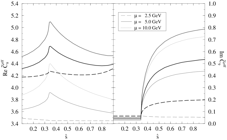
Figure 2: Comparison of the Wilson coefficient $\widetilde{C}_{9}^{eff}$ as a function of $\hat{s}$ for $m_{\rm t}=170\,{\rm GeV}$, $\Lambda_{\overline{\rm MS}}=0.225\,{\rm GeV}$ and different values of $\mu$ in leading order (thin lines) and next-to-leading order (thick lines) accuracy. Note the different scales for the real and imaginary parts!

In fig. 2 we show $\widetilde{C}_{9}^{eff}$ of (2.28) as a function of $\hat{s}$ for $m_{\rm t}=170\,{\rm GeV}$, $\Lambda_{\overline{\rm MS}}=225\,{\rm MeV}$ and $2.5\leq\mu\leq 10\,{\rm GeV}$. In order to see the importance of the term resulting from the one-loop matrix elements one should compare these results with the $\hat{s}$-independent values of $\widetilde{C}_{9}$. We should also remember that the NLO corrections to $P_{0}$ calculated here shift $\widetilde{C}_{9}^{eff}$ for $\mu=5.0\,{\rm GeV}$ by $\Delta\widetilde{C}_{9}^{NDR}\approx 0.8$ and $\Delta\widetilde{C}_{9}^{HV}\approx 0.6$ with similar results for other $\mu$. In order to show this effect more explicitly we also plot in fig. 2 a “leading order” result obtained by using only the leading term in (2.11) with $\alpha_{s}$ at the one-loop level but keeping otherwise all explicit NLO terms in (2.10) and the contributions from one-loop matrix elements given in (2.28). It should be stressed that roughly 50% of the difference between the “thick” and “thin” lines in fig. 2 is due to the term $4/9$ in (3.3) which in the NDR scheme enters the NLO terms in $P_{0}$ but in the HV scheme is present in the one-loop matrix elements. We have left it out in the “thin” lines in fig. 2 in order to show its importance. The calculation of NLO corrections to $P_{0}$ allows a consistent inclusion of this term which contributes positively to $\widetilde{C}_{9}^{eff}$. Additional enhancement comes from using the two-loop renormalization group analysis for $\widetilde{C}_{9}$ and $\alpha_{s}$ at the two-loop level. In fig. 2 we also note that $\mbox{Re}\widetilde{C}_{9}^{eff}\gg\mbox{Im}\widetilde{C}_{9}^{eff}$. The pronounced peak for $\hat{s}=4m_{\rm c}^{2}/m_{\rm b}^{2}=0.34$ is related to the behaviour of $h(z,\hat{s})$ in (2.31). This peak essentially disappears for $\mu=2.5\,{\rm GeV}$ because of the accidential cancellation $3C_{1}^{(0)}+C_{2}^{(0)}\approx 0$ in the dominant term multiplying $h(z,\hat{s})$. The authors of ref. [2] would find Re$\,\widetilde{C}_{9}^{eff}$ by about 15% below our values. In the absence of QCD corrections, $h(z,\hat{s})$ in (2.28) is multiplied by $C_{2}^{(0)}=1$ and consequently there is no accidental suppression of this term as in the QCD case. Since in addition for $\alpha_{s}\rightarrow 0$  $P_{0}^{NDR}$ is slightly enhanced over the values given in table 1, we find $\widetilde{C}_{9}^{eff}$ in the absence of QCD corrections to be substantially larger than the result given in fig. 2. For instance, Re $\widetilde{C}_{9}^{eff}$ varies between 5.2 and 6.3 for $0.1\leq\hat{s}\leq 0.9$. The complete result for $R(\hat{s})$ in this case is shown in fig. 5 at the end of this section.

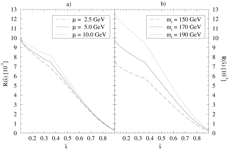
Figure 3: a) $R(\hat{s})$ for $m_{\rm t}=170\,{\rm GeV}$, $\Lambda_{\overline{\rm MS}}=225\,{\rm MeV}$ and different values of $\mu$.
Figure3: b) $R(\hat{s})$ for $\mu=5\,{\rm GeV}$, $\Lambda_{\overline{\rm MS}}=225\,{\rm MeV}$ and various values of $m_{\rm t}$.

We next present a numerical analysis of (2.27). In doing this we keep in mind that for $\hat{s}\approx m_{\psi}^{2}/m_{\rm b}^{2}$, $\hat{s}\approx m_{\psi^{\prime}}^{2}/m_{\rm b}^{2}$ etc. the spectator model cannot be the full story and additional long distance contributions discussed in refs. [14, 15, 16] have to be taken into account in a phenomenological analysis. Similarly we do not include $1/m_{\rm b}^{2}$ corrections calculated in [13] which typically enhance the differential rate by about 10%.

In fig. 3a) we show $R(\hat{s})$ for $m_{\rm t}=170\,{\rm GeV}$, $\Lambda_{\overline{\rm MS}}=225\,{\rm MeV}$ and different values of $\mu$. In fig. 3b) we set $\mu=5\,{\rm GeV}$ and vary $m_{\rm t}$ from $150\,{\rm GeV}$ to $190\,{\rm GeV}$. The remaining $\mu$ dependence is rather weak and amounts to at most $\pm 8\%$ in the full range of parameters considered. The $m_{\rm t}$ dependence of $R(\hat{s})$ is sizeable. Varying $m_{\rm t}$ between 150 GeV and 190 GeV changes $R(\hat{s})$ by typically 60–65% which in this range of $m_{\rm t}$ corresponds to $R(\hat{s})\sim m_{\rm t}^{2}$. It is easy to verify that this strong $m_{\rm t}$ dependence originates in the coefficient $\widetilde{C}_{10}$ given in (2.8) as already stressed by several authors in the past [1, 2, 3, 6, 8, 7, 4, 5].

We do not show the $\Lambda_{\overline{\rm MS}}$ dependence as it is very weak. Typically, changing $\Lambda_{\overline{\rm MS}}$ from $140\,{\rm MeV}$ to $310\,{\rm MeV}$ decreases $R(\hat{s})$ by about 5%.

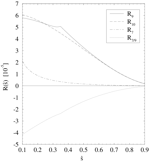
Figure 4: Comparison of the four different contributions to $R(\hat{s})$ according to eqn. (2.27).

$R(\hat{s})$ is governed by three coefficients, $\widetilde{C}_{9}^{eff}$, $\widetilde{C}_{10}$ and $C_{7}^{(0)eff}$. It is of interest to investigate the importance of various contributions. To this end we set $\Lambda_{\overline{\rm MS}}=225\,{\rm GeV}$, $m_{\rm t}=170\,{\rm GeV}$ and $\mu=5\,{\rm GeV}$. In fig. 4 we show $R(\hat{s})$ keeping only $\widetilde{C}_{9}^{eff}$, $\widetilde{C}_{10}$, $C_{7}^{(0)eff}$ and the $C_{7}^{(0)eff}$–$\widetilde{C}_{9}^{eff}$ interference term, respectively. Denoting these contributions by $R_{9}$, $R_{10}$, $R_{7}$ and $R_{7/9}$ we observe that the term $R_{7}$ plays only a minor role in $R(\hat{s})$. On the other hand the presence of $C_{7}^{(0)eff}$ cannot be ignored because the interference term $R_{7/9}$ is significant. In fact the presence of this large interference term could be used to measure experimentally the relative sign of $C_{7}^{(0)eff}$ and $\mbox{Re}\,\widetilde{C}_{9}^{eff}$ [2, 4, 5, 8, 7] which as seen in fig. 4 is negative in the Standard Model. However, the most important contributions are $R_{9}$ and $R_{10}$ in the full range of $\hat{s}$ considered. For $m_{\rm t}\approx 170\,{\rm GeV}$ these two contributions are roughly of the same size. Due to a strong $m_{\rm t}$ dependence of $R_{10}$, this contribution dominates for higher values of $m_{\rm t}$ and is less important than $R_{9}$ for $m_{\rm t}<170\,{\rm GeV}$.

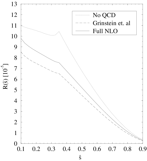
Figure 5: $R(\hat{s})$ for $m_{\rm t}=170\,{\rm GeV}$, $\Lambda_{\overline{\rm MS}}=225\,{\rm MeV}$ and $\mu=5\,{\rm GeV}$.

Next, in fig. 5 we show $R(\hat{s})$ for $\mu=5\,{\rm GeV}$, $m_{\rm t}=170\,{\rm GeV}$ and $\Lambda_{\overline{\rm MS}}=225\,{\rm MeV}$ compared to the case of no QCD corrections and to the results Grinstein et. al. [2] would obtain for our set of parameters using their approximate leading order formulae.

Finally, we would like to address the question of the definition of $m_{\rm t}$ used here. In order to be able to analyze this question, one would have to calculate perturbative QCD corrections to the functions $Y(x_{t})$ and $Z(x_{t})$ and include also an additional order in the renormalization group improved perturbative calculation of $P_{0}$. The latter would require evaluation of three-loop anomalous dimension matrices, which in the near future nobody will attempt. In any case, we expect only a small correction to $P_{0}$. The uncertainty due to the choice of $\mu$ in $m_{\rm t}(\mu)$ can be substantial, as stressed in refs. [33, 34], and may result in 20–30% uncertainties in the branching ratios. It can only be reduced if ${\cal O}(\alpha_{s})$ corrections to $Y(x_{t})$ and $Z(x_{t})$ are included. For $K^{+}\rightarrow\pi^{+}\nu\bar{\nu}$, $K_{L}\rightarrow\pi^{0}\nu\bar{\nu}$, $B\rightarrow\mu^{+}\mu^{-}$ and $B\rightarrow X_{s}\nu\bar{\nu}$ this has been done in refs. [33, 34]. The inclusion of these corrections reduces the uncertainty in the corresponding branching ratios to a few percent. Fortunately, the result for the corrected function $Y(x_{t})$ given in refs. [33, 34] can be directly used here. The message of refs. [33, 34] is the following: For $m_{\rm t}=\overline{m}_{\rm t}(m_{\rm t})$, the QCD corrections to $Y(x_{t})$ and consequently to $\widetilde{C}_{10}$ are below 2%. Corresponding corrections to $Z(x_{t})$ are not known. Fortunately, the $m_{\rm t}$ dependence of $\widetilde{C}_{9}$ is much weaker and the uncertainty due to the choice of $\mu$ in $m_{\rm t}(\mu)$ is small. On the basis of these arguments and the result of refs. [33, 34] we believe that if $m_{\rm t}=\overline{m}_{\rm t}(m_{\rm t})$ is chosen, the additional short distance QCD corrections to BR($B\rightarrow X_{s}e^{+}e^{-}$ ) should be small.

5 Summary

We have calculated the effective Hamiltonian relevant for the rare decay $B\rightarrow X_{s}e^{+}e^{-}$ beyond the leading logarithmic approximation. The main new result of this paper is the calculation of the Wilson coefficient of the operator $Q_{9}=(\bar{s}b)_{V-A}(\bar{e}e)_{V}$ including next-to-leading logarithms in the NDR and HV renormalization schemes. A separate analytic expression for $C_{9}$ given in sect. 2 as opposed to $C_{9}^{eff}$ given in [12] should be useful not only in $B\rightarrow X_{s}e^{+}e^{-}$ but also in $B\rightarrow K^{*}e^{+}e^{-}$ and other rare $B$-decays to which $Q_{9}$ contributes. Calculating $B\rightarrow X_{s}e^{+}e^{-}$ in the spectator model we confirm the very recent result for $C_{9}^{eff}$ presented by Misiak in [12]. The cancellation of the scheme dependence in $C_{9}^{eff}$ is shown explicitly in our paper.

The effect of the NLO corrections is to enhance BR($B\rightarrow X_{s}e^{+}e^{-}$ ) so that its suppression found in the leading order analysis of ref. [2] is considerably weakened. This is seen in particular in fig. 5.

We have investigated the $m_{\rm t}$, $\Lambda_{\overline{\rm MS}}$ and $\mu\approx{\cal O}(m_{\rm b})$ dependence of the “reduced” branching ratio $R(\hat{s})$. The dependences on $\Lambda_{\overline{\rm MS}}$ and $\mu$ are rather small, at most $\pm 8\%$ in the full range of parameters considered. The dependence on $m_{\rm t}$ is sizeable. In the range $150\,{\rm GeV}\leq m_{\rm t}\leq 190\,{\rm GeV}$ it is roughly parametrized by $R(\hat{s})\sim m_{\rm t}^{2}$. For $m_{\rm t}=170\,{\rm GeV}$, $\Lambda_{\overline{\rm MS}}=225\,{\rm MeV}$, $\mu=5\,{\rm GeV}$ and $0.1\leq\hat{s}\leq 0.8$ we find

$$1.0\cdot 10^{-5}\leq R(\hat{s})\leq 9.8\cdot 10^{-5}.$$ (5.13)

This result can be modified by non-perturbative $1/m_{\rm b}^{2}$ corrections and long distance contributions [14, 15, 16], which are however beyond the scope of this paper.

Acknowledgment

We would like to thank Mikołaj Misiak for the correspondence related to his independent analysis presented in ref. [12]. One of us (M.M.) appreciates helpful discussions with M. Jamin, M. Lautenbacher and U. Nierste.

References

- [1] W. S. Hou, R. I. Willey and A. Soni, Phys. Rev. Lett. 58 (1987) 1608.
- [2] B. Grinstein, M. J. Savage and M. B. Wise, Nucl. Phys. B319 (1989) 271.
- [3] S. Bertolini, F. Borzumati, A. Masiero and G. Ridolfi, Nucl. Phys. B353 (1991) 591.
- [4] A. Ali, T. Mannel, T. Morozumi, Phys. Lett. B273 (1991) 505.
- [5] W. Jaus and D. Wyler, Phys. Rev. D41 (1990) 3405.
- [6] N. G. Deshpande, K. Panose and J. Trampetić, Phys. Lett. B308 (1993) 322.
- [7] A. Ali, G. F. Giudice and T. Mannel, preprint CERN-TH 7346/94, hep-ph/9408213.
- [8] C. Greub, A. Ioannissian and D. Wyler, preprint ZU-TH 25/94, hep-ph/9408382.
- [9] R. Grigjanis, P. J. O’Donnell, M. Sutherland and H. Navelet, Phys. Lett. B223 (1989) 239.
- [10] G. Cella, G. Ricciardi and A. Viceré, Phys. Lett. B258 (1991) 212.
- [11] M. Misiak, Nucl. Phys. B393 (1993) 23.
- [12] M. Misiak, Erratum, to appear in Nucl. Phys.
- [13] A. Falk, M. Luke and M. J. Savage, Phys. Rev. D49 (1994) 3367.
- [14] C. S. Lim, T. Morozumi and A. I. Sanda, Phys. Lett. B218 (1989) 343.
- [15] N. G. Deshpande, J. Trampetić and K. Panose, Phys. Rev. D39 (1989) 1461.
- [16] P. J. O’Donnell and H. K. K. Tung, Phys. Rev. D43 (1991) R2067.
- [17] A. J. Buras, M. Jamin and M. E. Lautenbacher, Nucl. Phys. B408 (1993) 209.
- [18] A. J. Buras, M. Misiak, M. Münz and S. Pokorski, Nucl. Phys. B424 (1994) 374.
- [19] A. J. Buras, M. E. Lautenbacher, M. Misiak and M. Münz, Nucl. Phys. B423 (1994) 349.
- [20] G. ’t Hooft and M. Veltman, Nucl. Phys. B44 (1972) 189.
- [21] M. Ciuchini, E. Franco, G. Martinelli, L. Reina and L. Silvestrini, Phys. Lett. B316 (1993) 127.
- [22] M. Ciuchini, E. Franco, G. Martinelli and L. Reina, Nucl. Phys. B415 (1994) 403.
- [23] M. Ciuchini, E. Franco, L. Reina and L. Silvestrini, Nucl. Phys. B421 (1994) 41.
- [24] G. Cella, G. Curci, G. Ricciardi and A. Viceré, Nucl. Phys. B431 (1994) 417.
- [25] G. Cella, G. Curci, G. Ricciardi and A. Viceré, Phys. Lett. B325 (1994) 227.
- [26] N. Cabibbo and L. Maiani, Phys. Lett. B79 (1978) 109.
- [27] C. S. Kim and A. D. Martin, Phys. Lett. B225 (1989) 186.
- [28] M. Jeżabek and J. H. Kühn, Nucl. Phys. B320 (1989) 20.
- [29] R. Fleischer, private communication.
- [30] T. Inami and C. S. Lim, Prog. Theor. Phys. 65 (1981) 297.
- [31] A. J. Buras, M. Jamin, M. E. Lautenbacher and P. H. Weisz, Nucl. Phys. B400 (1993) 37.
- [32] M. Misiak, private communication.
- [33] G. Buchalla and A. J. Buras, Nucl. Phys. B398 (1993) 285.
- [34] G. Buchalla and A. J. Buras, Nucl. Phys. B400 (1993) 225.