Abstract

An upgraded analysis of $\epsilon$, $x_{d}$ and $\epsilon^{\prime}/\epsilon$, using the latest determinations of the relevant experimental and theoretical parameters, is presented. Using the recent determination of the top quark mass, $m_{t}=(174\pm 17)$ GeV, our best estimate is $\epsilon^{\prime}/\epsilon=3.1\pm 2.5$, which lies in the range given by E731. We describe our determination of $\epsilon^{\prime}/\epsilon$ and make a comparison with other similar studies. A detailed discussion of the matching of the full theory to the effective Hamiltonian, written in terms of lattice operators, is also given.

CERN-TH.7514/94

January 1995
^∗On leave of absence from Dip. di Fisica, Università degli Studi di Roma “La Sapienza”.

1 Introduction

The understanding of mixing and $CP$ violation in hadronic systems constitutes one of the crucial tests of the Standard Model. In the last few years considerable theoretical and experimental effort has been invested in this sector.

On the experimental side, more accurate measurements of the mixing angles are now available and the mass of the top quark, recently discovered, is constrained within tight limits [1]. Still, in spite of very accurate measurements, the experimental results for the $CP$ violating parameter $\epsilon^{\prime}/\epsilon$ are far from conclusive [2, 3].

On the theoretical side, the complete next-to-leading expressions of the relevant effective $\Delta S=1$, $\Delta S=2$, $\Delta B=1$ and $\Delta B=2$ Hamiltonians have been computed [4]–[8], thus reducing the theoretical uncertainties. Moreover, there is now increasing theoretical evidence that the value of the pseudoscalar $B$-meson decay constant is large, $f_{B}\sim 200$ MeV, and that the $B^{0}$–$\bar{B}^{0}$ mixing parameter $B_{B}$ is quite close to one. Still, the evaluation of other hadronic matrix elements is subject to large uncertainties, which are particularly severe for $\epsilon^{\prime}/\epsilon$, where important cancellations of different contributions occur, for large values of the top mass. A real improvement in the calculation of the hadronic matrix elements, from lattice simulations, or with other non-perturbative techniques, is still missing. In spite of this, we believe that, given the experimental and theoretical novelties, it is time to present an upgraded analysis of mixing and $CP$ violation for $K$- and $B$-mesons, along the lines followed in refs. [10, 11]. We will also have the opportunity of presenting our results for the Wilson coefficients of the operators appearing in the $\Delta S=1$ Hamiltonian in different regularization/renormalization schemes, which may be useful for further phenomenological analyses by other authors. We also intend to present and clarify several issues related to the matching conditions of effective Hamiltonians to the full theory, to the use of the lattice regularization, to the value of the mass of the strange quark and to quark thresholds in the evolution of the Wilson coefficients. Particular emphasis is devoted to a realistic evaluation of the uncertainties in our predictions.

The results given here contain several improvements with respect to our previous work on the same subject [11]. The main differences are the following:

• Upgraded values of the experimental parameters entering in the phenomenological analysis, such as the $B$-meson lifetime $\tau_{B}$, the $B^{0}_{d}$–$\bar{B}^{0}_{d}$ mixing parameter $x_{d}$, the CKM matrix elements, ($|V_{cb}|$, $|V_{ub}|/|V_{cb}|$), etc., have been used.

• The value of the strange quark mass $m_{s}$ has been taken from lattice calculations, thus making a more consistent use of lattice results for the $B$-parameters of the relevant penguin operators [12].

• The relevant formulae, necessary to express the effective Hamiltonian, derived in the full theory, are given in terms of lattice operators.

• Assumptions and relations which have been used to evaluate the $B$-parameters of the operators entering the calculation, in particular those that have not been computed either on the lattice, or with other non-perturbative techniques, are critically reviewed.

• Uncertainties, coming from the matching between lattice and continuum operators, are discussed, together with those due to the choice of the renormalization scale, $\Lambda_{QCD}$, the mass of the top quark, etc. We also discuss different determinations of $\epsilon^{\prime}/\epsilon$ originating from the choice of different continuum regularization schemes.

• All the results are presented with an estimate of the corresponding errors. These errors come from the limited precision of the measured quantities, e.g. $\tau_{B}$, and from theoretical uncertainties, e.g. the value of hadronic matrix elements.

The phenomenological results of this study have been partially reported elsewhere [13, 14]. In this paper we put particular emphasis on some theoretical aspects and subtleties related to the construction of the effective Hamiltonian. The reader will also find a practical tool to combine the Wilson coefficients with his own preferred results for the operator matrix elements, sections 4–6.

The plan of the paper is the following. We summarize in section 2 the main results obtained from a combined analysis of $\epsilon$, $x_{d}$ and $\epsilon^{\prime}/\epsilon$ together with our estimate of the errors. All the details of the analysis will be given after this section. In section 3, we give the relevant formulae of the effective Hamiltonians, which control $\epsilon$, $B^{0}$–$\bar{B}^{0}$ transitions and $\epsilon^{\prime}/\epsilon$, and define the relevant operators. In section 4, a summary of the calculation of the Wilson coefficients of the operators, at the next-to-leading order, is given. The matching of the continuum theory with the lattice is addressed in section 5. The formulae presented in this section have been used to derive the relation between the mass of the quarks on the lattice and in the continuum. In section 6 we give details on the Regularization Independent ($RI$) renormalization prescription, together with the numerical values of the Wilson coefficients in different renormalization schemes. In section 7, the values and errors of the $B$-parameters, used in this analysis, are given and compared with those used in ref. [15]. A discussion of the assumptions and relations among the $B$-parameters is also presented in the same section. The main uncertainties of the phenomenological analysis are reviewed in sec. 8.

2 Results

In this section, the main results of the present study are summarized. These results have been obtained by varying the experimental quantities, e.g. the value of the top mass $m_{t}$, $\tau_{B}$, etc., and the theoretical parameters, e.g. the kaon $B$-parameter $B_{K}$ or the strange quark mass $m_{s}^{\overline{MS}}(\mu)$, according to their errors. Values and errors of the input quantities, used in the following, are reported in tables 1– 3. For the experimental quantities, we assume a Gaussian distribution and, for the theoretical ones, a flat distribution (with a width of $2\,\sigma$). The only exception is $m_{s}^{\overline{MS}}(\mu)$, taken from quenched lattice $QCD$ calculations, for which we have assumed a Gaussian distribution, according to the results of ref. [12].

Each theoretical prediction ($\cos\delta$, $\sin 2\beta$, $\epsilon^{\prime}/\epsilon$, etc.), depends on several input parameters, which fluctuate independently. In many cases, this produces a pseudo-Gaussian distribution of values, see for example $\epsilon^{\prime}/\epsilon$ in fig. 1. From the width of the pseudo-Gaussian, we estimate the errors of our predictions. Non-Gaussian distributions may also occur, for example when a single input parameter dominates the result. In these cases, we still estimate the error from the variance of the distribution.

Parameters	Values
$m_{t}$	$(174\pm 17)$ GeV
$m_{s}$(2 GeV)	($128\pm 18$) MeV
$\Lambda_{QCD}^{n_{f}=5}$	($230\pm 80$) MeV
$V_{cb}=A\lambda^{2}$	$0.040\pm 0.006$
$|V_{ub}/V_{cb}|=\lambda\sigma$	$0.080\pm 0.015$
$\tau_{B}$	$(1.49\pm 0.12)\times 10^{-12}$ sec
$x_{d}$	$0.685\pm 0.076$
$(f_{B}B_{B}^{1/2})_{th}$	$(200\pm 40)$ MeV
$\Omega_{IB}$	$0.25\pm 0.10$

Table 1: Values and errors of the parameters used in the numerical analysis.

Constants	Values
$G_{F}$	$1.16634\times 10^{-5}\mbox{GeV}^{-2}$
$m_{c}$	1.5 GeV
$m_{b}$	4.5 GeV
$M_{W}$	80.2 GeV
$M_{\pi}$	140 MeV
$M_{K}$	490 MeV
$M_{B}$	5.278 GeV
$\Delta M_{K}$	$3.521\times 10^{-12}$ MeV
$f_{\pi}$	132 MeV
$f_{K}$	160 MeV
$\lambda=\sin\theta_{c}$	0.221
$\epsilon_{exp}$	$2.268\times 10^{-3}$
$\mbox{Re}A_{0}$	$2.7\times 10^{-7}$ GeV
$\omega$	0.045
$\mu$	$2$ GeV

Table 2: Constants used in the numerical analysis.

$B_{K}$	$B_{9}^{(3/2)}$	$B_{1-2}^{c}$	$B_{3,4}$	$B_{5,6}$	$B_{7-8-9}^{(1/2)}$	$B_{7-8}^{(3/2)}$
$0.75\pm 0.15$	$0.62\pm 0.10$	$0-0.15^{(*)}$	$1-6^{(*)}$	$1.0\pm 0.2$	$1^{(*)}$	$1.0\pm 0.2$

Table 3: Values of the $B$-parameters, for operators renormalized at the scale $\mu=2$ GeV. The only exception is $B_{K}$, which is the renormalization group-invariant $B$-parameter, defined in ref. [18]; $B_{9}^{3/2}(\mu)$ has been taken equal to $B_{K}(\mu)$, at any renormalization scale $\mu$. In the table, we give $B_{9}^{3/2}(\mu=2$ GeV$)$. Entries with a ^(∗) are educated guesses; the others are taken from lattice $QCD$ calculations [19]–[32]. See section 7 for more details.

Using the numbers given in the tables and the formulae given in the forthcoming section, we have obtained the following results:

a) The comparison of the experimental value of $\epsilon$ with its theoretical prediction will in general correspond to two possible solutions for the value of $\cos\delta$, see for example ref. [10]. Because of the errors of the input parameters, the two solutions appear as a distribution of values, with a twin-peak shape. The distribution for $\cos\delta$ is given in fig. 1. As already noticed in refs. [10, 11] and [16, 17], a large value of $f_{B}$, combined with a large $m_{t}$, favours $\cos\delta>0$. When the condition $160$ MeV $\leq f_{B}B_{B}^{1/2}\leq 240$ MeV is imposed ($f_{B}$-cut), most of the negative solutions disappear, giving the dashed histogram of fig. 1, from which we estimate

$$\cos\delta=0.47\pm 0.32\,\,.$$ (1)

b) $\cos\delta$ is correlated to the values of the Wolfenstein parameters $\rho$ and $\eta$. In fig. 2, the contour plot in the $\rho$–$\eta$ plane is given, with and without the $f_{B}$-cut.

Figure 1: Distributions of values for $\cos\delta$, $\sin 2\beta$, $\epsilon^{\prime}/\epsilon$ and $\epsilon^{\prime}/\epsilon(A^{2}\eta)^{-1}$, for $m_{t}=(174\pm 17)$ GeV, and using the values of the parameters given in tables 1– 3. The solid histograms are obtained without using the information coming from $B_{d}$–$\bar{B}_{d}$ mixing, the dashed ones after imposing that $160$ MeV $\leq f_{B}B_{B}^{1/2}\leq 240$ MeV.

Figure 2: Contour plots in the $\rho$–$\eta$ plane. The solid, dashed and dotted contours contain $5\%$, $68\%$ and $95\%$ of the generated events respectively. The contours are given by excluding or including the $f_{B}$-cut. Similar results can be found in refs. [16, 17].

c) The value of $\sin 2\beta$ depends on $\cos\delta$

$$\sin 2\beta=\frac{2\sigma\sin\delta(1-\sigma\cos\delta)}{1+\sigma^{2}-2\sigma\cos\delta}.$$ (2)

The distribution of $\sin 2\beta$ is shown in fig. 1, without (solid) and with (dashed) the $f_{B}$-cut. When the $f_{B}$-cut is imposed, one gets larger values of $\sin 2\beta$ [10].

Figure 3: Distributions of the events in the plane $\epsilon^{\prime}/\epsilon$–$\cos\delta$ without and with the $f_{B}$-cut. The corresponding contour plots are displayed below the lego-plots.

From the dashed distribution, we obtain

$$\sin 2\beta=0.65\pm 0.12\,\,.$$ (3)

d) In fig. 3, several pieces of information on $\epsilon^{\prime}/\epsilon$ are provided. Lego-plots of the distribution of the generated events in the $\epsilon^{\prime}/\epsilon$–$\cos\delta$ plane are shown, without and with the $f_{B}$-cut. At the same time, the corresponding contour plots are displayed. One notices a very mild dependence of $\epsilon^{\prime}/\epsilon$ on $\cos\delta$. As a consequence, one obtains approximately the same prediction in the two cases (see also fig. 1). In the $HV$ scheme [33] the results are

$$\epsilon^{\prime}/\epsilon=(2.3\pm 2.1)\times 10^{-4}\,\,\,\hbox{No-cut},$$ (4)

and

$$\epsilon^{\prime}/\epsilon=(2.8\pm 2.4)\times 10^{-4}\,\,\,f_{B}\hbox{-cut},$$ (5)

whereas in the $NDR$ scheme they become

$$\epsilon^{\prime}/\epsilon=(2.8\pm 2.2)\times 10^{-4}\,\,\,\hbox{No-cut},$$ (6)

and

$$\epsilon^{\prime}/\epsilon=(3.4\pm 2.5)\times 10^{-4}\,\,\,f_{B}\hbox{-cut}.$$ (7)

Our best estimate, reported in the abstract, has been obtained by averaging the results given in eqs.(5) and (7) and by adding a systematic error, due to the difference of the central values in the two schemes, to the final result

$$\epsilon^{\prime}/\epsilon=(3.1\pm 2.5\pm 0.3)\times 10^{-4}\,\,\,f_{B}\hbox{-cut}.$$ (8)

e) In view of the rapid evolution of the experimental determination of the value of the top mass, expected in the near future, we also give $\epsilon^{\prime}/\epsilon$ as a function of $m_{t}$, in fig. 4.

\begin{picture}(6.0,7.0)\put(-6.0,-7.0){} \end{picture}

Figure 4: $\epsilon^{\prime}/\epsilon$ as a function of $m_{t}$, obtained by applying the $f_{B}$-cut. The zones delimited by the solid and dashed curves represent the allowed regions containing respectively $68\%$ and $95\%$ of the generated events. The region between the two double lines is the experimental result coming from E731 [3], $\epsilon^{\prime}/\epsilon=(7.4\pm 5.9)\times 10^{-4}$. The range from NA31 [2], $\epsilon^{\prime}/\epsilon=(23.0\pm 6.5)\times 10^{-4}$ is not given in the figure.

By comparing the present results to the analysis of ref. [11], one may notice the following:

1. The latest values of $|V_{ub}/V_{cb}|$ and $|V_{cb}|$ are sensibly lower than the previous ones. Consequently, the separation of the positive–negative $\cos\delta$ solutions takes place at larger values of $m_{t}$.

2. $\epsilon^{\prime}/\epsilon\sim|V_{ub}/V_{cb}|\times|V_{cb}|^{2}$. The actual results for $\epsilon^{\prime}/\epsilon$, however, are not very different from those given in ref. [11], because we are now using a smaller value of the strange quark mass taken from lattice $QCD$ [12], and not from $QCD$ sum rules [34]–[39], as we did before. One has new reasons to doubt of those $QCD$ sum rule determinations, which have been found to be affected by large higher order [40] or instanton effects [41]. It is reassuring that the recent $QCD$ sum rule calculation of ref. [42], apparently free of uncontrolled non-perturbative effects, agrees with the lattice calculation of ref. [12].

3. In spite of several differences, the bulk of our results overlaps with those of ref. [15]. It is encouraging that theoretical predictions, obtained by using different approaches to evaluate the operator matrix elements, are in good agreement.

4. On the basis of the latest analyses, it seems very difficult that $\epsilon^{\prime}/\epsilon$ is larger than $10\times 10^{-4}$. Theoretically, this may happen by taking the matrix elements of the dominant operators, $Q_{6}$ and $Q_{8}$ (see below) very different from usually assumed. One possibility, discussed in ref. [15], is to take the corresponding $B$-parameters to be $B_{6}\sim 2$ and $B_{8}\sim 1$, instead of the values $B_{6}\sim B_{8}\sim 1$, adopted here and in refs. [10, 11, 15]. To our knowledge, no coherent theoretical approach has found $B_{6}$ so large, and we see no reason to use $B_{6}=2$.

3 $\epsilon$, $B^{0}-\bar{B}^{0}$ transitions and $\epsilon^{\prime}/\epsilon$

In this section, we list the expressions of the effective Hamiltonians, responsible for $\Delta S\!=\!2$, $\Delta B=2$ and $\Delta S\!=\!1$ transitions, given in terms of the relevant operators and their Wilson coefficients. From these Hamiltonians, one derives the expressions for $\epsilon$, $x_{d}$ and $\epsilon^{\prime}/\epsilon$, written as combinations of the Wilson coefficients times the $B$-parameters of the different operators, i.e. their matrix elements. The formulae of this section have been used in our study.

1) The effective Hamiltonian governing the $\Delta S\!=\!2$ amplitude is given by

$${\cal H}_{eff}^{|\Delta S|=2}=\frac{G_{F}^{2}}{16{\pi}^{2}}M_{W}^{2}({\bar{d}}{\gamma}^{\mu}_{L}s)^{2}\left\{{\lambda}_{c}^{2}F(x_{c})+{\lambda}_{t}^{2}F(x_{t})+2{\lambda}_{c}{\lambda}_{t}F(x_{c},x_{t})\right\},$$

where $G_{F}$ is the Fermi coupling constant and $\gamma^{\mu}_{L}=\gamma^{\mu}(1-\gamma_{5})\,$; ${\lambda}_{q}$’s are related to the CKM matrix elements by ${\lambda}_{q}=V_{qi}V^{\star}_{qf}$, where ‘$i$’ and ‘$f$’ are the labels of the initial and final states respectively (in the present case $i=s$ and $f=d$); $x_{q}={m_{q}^{2}}/{M_{W}^{2}}~{}$ and the functions $F(x_{i})$ and $F(x_{i},x_{j})$ are the so-called Inami-Lim functions [43], obtained from the calculation of the basic box-diagram and including $QCD$ corrections [44]; $F(x_{t})$ is known at the next-to-leading order, which has been included in our calculation. From equation (LABEL:effective_hamiltonian1) we can derive the CP violation parameter $\epsilon$

$$|\epsilon|_{\xi=0}=C_{\epsilon}B_{K}A^{2}\lambda^{6}\sigma\sin\delta\left\{F(x_{c},x_{t})+F(x_{t})[A^{2}\lambda^{4}(1-\sigma\cos\delta)]-F(x_{c})\right\},$$

where

$$C_{\epsilon}=\frac{G_{F}^{2}f_{K}^{2}M_{K}M_{W}^{2}}{6\sqrt{2}{\pi}^{2}\Delta M_{K}}.$$ (11)

Here, $\Delta M_{K}$ is the mass difference between the two neutral kaon mass eigenstates. In eq. (LABEL:epsilon_csizero_1), $\rho=\sigma\cos\delta$, $\eta=\sigma\sin\delta$ and $\lambda$, $A$, $\rho$ and $\eta$ are the parameters of the CKM matrix in the Wolfenstein parametrization [45]; $B_{K}$ is the renormalization group-invariant $B$-factor, to be discussed in sec. 7; $B_{K}$ takes into account all the possible deviations from the vacuum insertion approximation in the evaluation of the matrix element $\langle{\bar{K}}^{0}|(\bar{d}\gamma^{\mu}_{L}s)^{2}|K^{0}\rangle$ ($B_{K}=1$ corresponding to the vacuum insertion approximation).

2) The $\Delta B=2$ effective Hamiltonian is given by

$${\cal H}_{eff}^{|\Delta B|=2}=\frac{G_{F}^{2}}{16{\pi}^{2}}M_{W}^{2}{\lambda}_{t}^{2}({\bar{d}}{\gamma}^{\mu}_{L}b)^{2}F(x_{t}),$$

from which one finds

$$x_{d} = \frac{\Delta M}{\Gamma}=C_{B}\frac{\tau_{B}f_{B}^{2}}{M_{B}}B_{B}A^{2}\lambda^{6}\Bigl{(}1+\sigma^{2}-2\sigma\cos\delta\Bigr{)}F(x_{t}),$$

$$C_{B} = \frac{G_{F}^{2}M_{W}^{2}M_{B}^{2}}{6\pi^{2}},$$ (13)

where $B_{B}$ is the renormalization-invariant $B$-parameter, relevant for $B$–$\bar{B}$ mixing.

3) The $\Delta S=1$ effective Hamiltonian above the charm threshold is given by

$${\cal H}_{eff}^{\Delta S\!=\!1} = \lambda_{u}\frac{G_{F}}{\sqrt{2}}\Bigl{[}(1-\tau)\Bigl{(}C_{1}(\mu)\left(Q_{1}(\mu)-Q_{1}^{c}(\mu)\right)+C_{2}(\mu)\left(Q_{2}(\mu)-Q_{2}^{c}(\mu)\right)\Bigr{)}$$ (14)

$$+ \tau\vec{Q}(\mu)^{T}\cdot\vec{C}(\mu)\Bigr{]}$$

where $\vec{Q}(\mu)=(Q_{1}(\mu),Q_{2}(\mu),\dots)$, $\vec{C}(\mu)=(C_{1}(\mu),C_{2}(\mu),\dots)$, $\lambda_{u}=V_{ud}V^{*}_{us}$ and similarly $\lambda_{c}$ and $\lambda_{t}$; $\tau=-\lambda_{t}/\lambda_{u}$ and $\mu$ is the renormalization scale of the operators $Q_{i}$. A convenient basis of operators [46]–[49], when $QCD$ and $QED$ corrections are taken into account, is

$$Q_{1} = ({\bar{s}}_{\alpha}d_{\alpha})_{(V-A)}({\bar{u}}_{\beta}u_{\beta})_{(V-A)}$$

$$Q_{2} = ({\bar{s}}_{\alpha}d_{\beta})_{(V-A)}({\bar{u}}_{\beta}u_{\alpha})_{(V-A)}$$

$$Q_{3,5} = ({\bar{s}}_{\alpha}d_{\alpha})_{(V-A)}\sum_{q}({\bar{q}}_{\beta}q_{\beta})_{(V\mp A)}$$

$$Q_{4,6} = ({\bar{s}}_{\alpha}d_{\beta})_{(V-A)}\sum_{q}({\bar{q}}_{\beta}q_{\alpha})_{(V\mp A)}$$

$$Q_{7,9} = \frac{3}{2}({\bar{s}}_{\alpha}d_{\alpha})_{(V-A)}\sum_{q}e_{q}({\bar{q}}_{\beta}q_{\beta})_{(V\pm A)}$$

$$Q_{8,10} = \frac{3}{2}({\bar{s}}_{\alpha}d_{\beta})_{(V-A)}\sum_{q}e_{q}({\bar{q}}_{\beta}q_{\alpha})_{(V\pm A)}$$

$$Q^{c}_{1} = ({\bar{s}}_{\alpha}d_{\alpha})_{(V-A)}({\bar{c}}_{\beta}c_{\beta})_{(V-A)}$$

$$Q^{c}_{2} = ({\bar{s}}_{\alpha}d_{\beta})_{(V-A)}({\bar{c}}_{\beta}c_{\alpha})_{(V-A)}$$ (15)

where the subscript $(V\pm A)$ indicates the chiral structure and $\alpha$ and $\beta$ are colour indices. The sum over the quarks $q$ runs over the active flavours at the scale $\mu$.

From ${\cal H}_{eff}^{|\Delta S=1|}$ we can derive the expression for $\epsilon^{\prime}$

$$\epsilon^{\prime}=\frac{e^{i\pi/4}}{\sqrt{2}}\frac{\omega}{\mbox{Re}\,A_{0}}\left[\omega^{-1}(\mbox{Im}\,A_{2})^{\prime}-(1-\Omega_{IB})\,\mbox{Im}\,A_{0}\right],$$ (16)

where $(\mbox{Im}\,A_{2})^{\prime}$ and $\mbox{Im}\,A_{0}$ are given by

$$\mbox{Im}\,A_{0} = -\frac{G_{F}}{\sqrt{2}}\mbox{Im}\,\Bigl{(}{V}_{ts}^{*}{V}_{td}\Bigr{)}\left\{-\left(C_{6}B_{6}+\frac{1}{3}C_{5}B_{5}\right)Z+\left(C_{4}B_{4}+\frac{1}{3}C_{3}B_{3}\right)X+\right.$$ (17)

$$\!C_{7}B_{7}^{1/2}\left(\frac{2Y}{3}+\frac{Z}{6}+\frac{X}{2}\right)+C_{8}B_{8}^{1/2}\left(2Y+\frac{Z}{2}+\frac{X}{6}\right)-$$

$$\!\left.C_{9}B_{9}^{1/2}\frac{X}{3}+\left(\frac{C_{1}B_{1}^{c}}{3}+C_{2}B_{2}^{c}\right)X\right\},$$

and

$$(\mbox{Im}\,A_{2})^{\prime}\! = \!-G_{F}\mbox{Im}\,\Bigl{(}{V}_{ts}^{*}{V}_{td}\Bigr{)}\left\{C_{7}B_{7}^{3/2}\left(\frac{Y}{3}-\frac{X}{2}\right)+\right.$$ (18)

$$\!\left.C_{8}B_{8}^{3/2}\left(Y-\frac{X}{6}\right)+C_{9}B_{9}^{3/2}\frac{2X}{3}\right\}.$$

$\omega=\mbox{Re}\,A_{2}/\mbox{Re}\,A_{0}=0.045$ and we have introduced $(\mbox{Im}\,A_{2})^{\prime}$ defined as

$$\mbox{Im}\,A_{2}=(\mbox{Im}\,A_{2})^{\prime}+\Omega_{IB}(\omega\,\mbox{Im}\,A_{0}).$$ (19)

$\Omega_{IB}=0.25\pm 0.10$ represents the isospin breaking contribution, see for example ref. [50]. With the subtle cancellations, occurring for a large top mass, $m_{t}\sim 175$ GeV, a precise knowledge of the value of $\Omega_{IB}$ becomes important. For example, by taking $\Omega_{IB}=0$, one gets $\epsilon^{\prime}/\epsilon\sim 5\times 10^{-4}$, instead of $2.8\times 10^{-4}$. In view of this, further efforts should be devoted to improve the accuracy of the theoretical predictions for isospin-breaking effects.

The numerical evaluation of $\epsilon^{\prime}/\epsilon$ requires the knowledge of the Wilson coefficients of the operators and of the corresponding matrix elements. The Wilson coefficients have been evaluated at the next-to-leading order, using the anomalous dimension matrices given in refs. [4]–[8], and the initial conditions computed in refs. [51, 52] (and given for $HV$ and $NDR$ in refs. [6]–[8]). The matrix elements of the operators have been written in terms of the three quantities (see eqs. (17) and (18))

$$X\! = \!f_{\pi}\left(M_{K}^{2}-M_{\pi}^{2}\right),$$ (20)

$$Y\! = \!f_{\pi}\left(\frac{M_{K}^{2}}{m_{s}(\mu)+m_{d}(\mu)}\right)^{2}\sim 12\,X\left(\frac{0.15\,\mbox{GeV}}{m_{s}(\mu)}\right)^{2},$$ (21)

$$Z\! = \!4\left(\frac{f_{K}}{f_{\pi}}-1\right)Y,$$ (22)

and a set $\{B_{i}\}$ of $B$-parameters (in our normalization $f_{\pi}=132$ MeV). The numerical value of the $B$-parameters have been taken from lattice calculations [19]–[32] and multiplied by suitable renormalization factors to take into account the difference between $HV$ ($NDR$) and the lattice regularization scheme. For those $B$-factors that have not been computed yet on the lattice we have used an educated guess, which will be discussed in detail in the following. We observe that, in eqs. (17) and (18), only nine coefficients ($B$-parameters) appear since we have used the relation $Q_{10}=-Q_{3}+Q_{4}+Q_{9}$, which is valid below the bottom threshold.

4 Wilson expansion and renormalization

This section is devoted to the Wilson coefficients of the operators appearing in the effective $\Delta S=1$ Hamiltonian, which we have computed at the next-to-leading order, including $QCD$ and $QED$ corrections. We do not discuss the determination of the coefficients of the operators relevant for $\epsilon$, since this point was explained in great detail in ref. [10].

The effective Hamiltonian is defined by the Wilson Operator Product Expansion (OPE) of the $T$-product of two weak currents:

$$\langle F|{\cal H}_{eff}^{|\Delta S=1|}|I\rangle = g_{W}^{2}/8\int d^{4}xD^{\mu\nu}_{W}(x^{2},M_{W}^{2})\langle F|T\left(J_{\mu}(x),J^{\dagger}_{\nu}(0)\right)|I\rangle$$ (23)

$$\rightarrow \sum_{i}C_{i}(M_{W})\langle F|Q_{i}(M_{W})|I\rangle.$$

The Wilson coefficients $\vec{C}(M_{W})=(C_{1}(M_{W}),C_{2}(M_{W})...)$ are found by matching, at $O(\alpha_{e})$ and $O(\alpha_{s})$, the current–current and penguin diagrams computed with the $W$ and top propagators to those computed with the local four-fermion operators in the effective theory. The $\vec{C}(\mu)$ are expressed in terms of $\vec{C}(M_{W})$ through the renormalization evolution matrix $\hat{W}[\mu,M_{W}]$

$$\vec{C}(\mu)=\hat{W}[\mu,M_{W}]\vec{C}(M_{W}),$$ (24)

where

$$\hat{W}[\mu,M_{W}]=\hat{M}[\mu]\hat{U}[\mu,M_{W}]\hat{M}^{\prime}[M_{W}],$$ (25)

with

$$\hat{M}[\mu]=\left(\hat{1}+\frac{\alpha_{e}}{4\pi}\hat{K}\right)\left(\hat{1}+\frac{\alpha_{s}(\mu)}{4\pi}\hat{J}\right)\left(\hat{1}+\frac{\alpha_{e}}{\alpha_{s}(\mu)}\hat{P}\right)$$ (26)

and

$$\hat{M}^{\prime}[M_{W}]=\left(\hat{1}-\frac{\alpha_{e}}{\alpha_{s}(M_{W})}\hat{P}\right)\left(\hat{1}-\frac{\alpha_{s}(M_{W})}{4\pi}\hat{J}\right)\left(\hat{1}-\frac{\alpha_{e}}{4\pi}\hat{K}\right).$$ (27)

At the next-to-leading accuracy, $\hat{W}[\mu,M_{W}]$ is regularization scheme dependent.

We now give the basic information necessary to compute the matrices defined in eqs. (25), (26) and (27).

The matrix $\hat{U}[\mu,M_{W}]$ in eq. (25) is given by

$$\hat{U}[\mu,M_{W}]=\left[\frac{\alpha_{s}(M_{W})}{\alpha_{s}(\mu)}\right]^{\hat{\gamma}^{(0)T}_{s}/2\beta_{0}}\,.$$ (28)

The matrices $\hat{P}$, $\hat{J}$ and $\hat{K}$ are solutions of the equations

$$\hat{P}+\left[\hat{P},\frac{\hat{\gamma}^{(0)T}_{s}}{2\beta_{0}}\right]=\frac{\hat{\gamma}^{(0)T}_{e}}{2\beta_{0}}$$ (29)

$$\hat{J}-\left[\hat{J},\frac{\hat{\gamma}^{(0)T}_{s}}{2\beta_{0}}\right]=\frac{\beta_{1}}{2\beta^{2}_{0}}\hat{\gamma}^{(0)T}_{s}-\frac{\hat{\gamma}^{(1)T}_{s}}{2\beta_{0}}$$ (30)

$$\left[\hat{K},\hat{\gamma}^{(0)T}_{s}\right]=\hat{\gamma}^{(1)T}_{e}+\hat{\gamma}^{(0)T}_{e}\hat{J}+\hat{\gamma}^{(1)T}_{s}\hat{P}+\left[\hat{\gamma}^{(0)T}_{s},\hat{J}\hat{P}\right]-2\beta_{1}\hat{P}-\frac{\beta_{1}}{\beta_{0}}\hat{P}\hat{\gamma}^{(0)T}_{s}\,.$$ (31)

The anomalous dimension matrix, which includes gluon and photon corrections, can be written as

$$\hat{\gamma}=\frac{\alpha_{s}}{4\pi}\hat{\gamma}_{s}^{(0)}+\frac{\alpha_{e}}{4\pi}\hat{\gamma}_{e}^{(0)}+\Bigl{(}\frac{\alpha_{s}}{4\pi}\Bigr{)}^{2}\hat{\gamma}_{s}^{(1)}+\frac{\alpha_{s}}{4\pi}\frac{\alpha_{e}}{4\pi}\hat{\gamma}_{e}^{(1)}\,,$$ (32)

where each of the $\hat{\gamma}^{(0,1)}_{s,e}$ is a $10\times 10$ matrix. In eqs. (28)–(31), $\beta_{0}$ and $\beta_{1}$ are the first two coefficients of the $\beta$-function of $\alpha_{s}$. At the leading order, the $QCD$ anomalous dimension matrix, including $QCD$ penguins, has been computed in refs. [46, 47]. The electroweak anomalous dimension matrix at the same order can be found in refs. [48], [49] and [52]. Two groups have computed the anomalous dimension matrix at the next-to-leading order, by calculating all the current–current and penguin operators at two loops up to order $\alpha_{s}^{2}t$ and $\alpha_{e}\alpha_{s}t$ [6]–[8]. All the details of the computation can be found in these references. Here we only give the numerical results for the Wilson coefficients in three different regularization/renormalization schemes, which are commonly used in the literature, namely $HV$, $NDR$ and $RI$:

1. $HV$ denotes the $\overline{MS}$ renormalization prescription in dimensional regularization, with $\gamma_{5}$ defined according to the ’t Hooft and Veltman prescription [33];

2. $NDR$ is the $\overline{MS}$ scheme in Naïve Dimensional Regularization, with anticommuting $\gamma_{5}$;

3. The $RI$ (Regularization Independent) scheme requires a few words of explanation. In its simplest realization, one fixes the renormalization conditions of a certain operator, by imposing that suitable Green functions, computed between external off-shell quark and gluon states, in a fixed gauge, coincide with their tree level value. For example, if we consider the generic two-quark operator $O_{\Gamma}=\bar{\psi}\Gamma\psi$, we may impose the condition

   $$Z_{\Gamma}\langle p|O_{\Gamma}|p\rangle|_{p^{2}=-\mu^{2}}=\langle p|O_{\Gamma}|p\rangle_{0},$$ (33)

   where $\Gamma$ is one of the Dirac matrices and $\langle p|O_{\Gamma}|p\rangle_{0}$ is the tree level matrix element. The extension to more complicated cases, including four-fermion operators and operator mixing, is straightforward and will be discussed in detail in sec. 6. The $RI$ procedure defines the same renormalized operators, i.e. the same coefficients, in all regularization schemes ($HV$, $NDR$, Pauli–Villars, lattice), provided they are expressed in terms of the same renormalized strong coupling constant. However, the coefficient functions now depend on the external states and on the gauge used to impose the renormalization conditions. Thus the external states and the gauge must be specified. To make contact with the non-perturbative method proposed in ref. [53], we will use the Landau gauge. The external states will be different for different operators, and will be given in sec. 6.

   The $RI$ scheme is particularly convenient for matching the coefficients of the operators to the corresponding matrix elements computed in lattice simulations, as extensively discussed in ref. [53]. The details of the implementation of this renormalization scheme will be given in sec. 6, where we also present the relations between the renormalized operators and coefficients computed with the RI scheme and with the usual $\overline{MS}$ prescriptions.

5 The effective Hamiltonian written in terms of lattice operators

Hadronic matrix elements from lattice $QCD$ have been widely used to predict several quantities of phenomenological interest in weak decays, deep inelastic scattering and heavy flavour physics. In this section we discuss the renormalization properties of lattice operators and clarify some issues related to the construction of physical amplitudes starting from the matrix elements computed on the lattice. For definiteness and simplicity, we will refer to two-fermion operators and to the four-fermion $\Delta I=3/2$ operator $Q^{+}$, which renormalize multiplicatively in the continuum. The relations derived below are, however, valid in the general case. These relations have been used to compute the strange and charm quark masses in ref. [12].

Let us consider first the renormalization of the generic two-quark operator $\bar{\psi}\Gamma\psi$, where $\Gamma$ is one of the Dirac matrices. At the next-to-leading order (NLO), the generic, forward, two-point Green function, computed between quark states of virtuality $p^{2}=\mu^{2}$, has the form

$$\Gamma(\mu a) = \Gamma_{0}\left\{1+\frac{g^{2}_{L}(a)}{16\pi^{2}}\left(\frac{\gamma^{(0)}}{2}\ln\left(\frac{\mu a}{\pi}\right)^{2}+C^{L}\right)\right.$$

$$+ \Bigl{(}\frac{g^{2}_{L}(a)}{16\pi^{2}}\Bigr{)}^{2}\left[\frac{1}{8}\gamma^{(0)}(-2\beta_{0}+\gamma^{(0)})\ln^{2}\left(\frac{\mu a}{\pi}\right)^{2}\right.$$

$$+ \left.\left.\frac{1}{2}\left(\bar{\gamma}^{(1)}+(-2\beta_{0}+\gamma^{(0)})C^{L}+\beta^{0}_{\lambda}\left(\lambda\frac{\partial C^{L}}{\partial\lambda}\right)\right)\ln\left(\frac{\mu a}{\pi}\right)^{2}\right]\right\}+\dots$$

where the dots represent terms beyond the next-to-leading order and terms of $O(a)$, which we will assume negligible in the following; $\Gamma_{0}$ is the zeroth-order Green function, and $g^{2}_{L}(a)=6/\beta$ is the bare lattice coupling constant; $\gamma^{(0)}$ and $\bar{\gamma}^{(1)}$ are the leading (regularization-independent) and next-to-leading (regularization-dependent) order anomalous dimensions, respectively; $\lambda=\lambda(a)$ is the lattice gauge parameter of the gluon propagator $\Bigl{(}\Pi_{\mu\nu}(q^{2})=-\delta_{\mu\nu}+(1-\lambda)q_{\mu}q_{\nu}/q^{2}\Bigr{)}$. It obeys the renormalization group equation

$$\frac{1}{\lambda(a)}a\frac{\partial\lambda(a)}{\partial a}=-\beta_{\lambda}(g^{2}_{L}(a))=-\beta^{0}_{\lambda}\frac{g^{2}_{L}(a)}{16\pi^{2}}+\cdots,\,\,\,\,\,\,\,\,\,\beta^{0}_{\lambda}=\frac{5N-2n_{f}}{6\pi}.$$ (35)

We have introduced a scale-dependent gauge parameter in order to define a gauge-independent anomalous dimension and simplify the renormalization group equation for $\Gamma(\mu a)$, see eq. (38) below.

The lattice coupling constant obeys the equation

$$a\frac{dg^{2}_{L}(a)}{da}=-\beta(g^{2}_{L}(a))=2\beta_{0}\frac{g^{4}_{L}(a)}{16\pi^{2}}+2\beta_{1}\frac{g^{6}_{L}(a)}{(16\pi^{2})^{2}},$$ (36)

where $\beta_{0,1}$ are given by

$$\beta_{0}=\frac{(11N-2n_{f})}{3},\,\,\,\,\,\,\,\,\,\,\,\beta_{1}=\frac{34}{3}N^{2}-\frac{10}{3}Nn_{f}-\frac{(N^{2}-1)}{N}n_{f}$$ (37)

and $n_{f}$ is the number of flavours. Equation (34) guarantees that all the matrix elements can be made finite (as $a\rightarrow 0$) by multiplying the bare operator by a suitable renormalization constant, obtained by fixing the renormalization conditions for $O_{\Gamma}$.

From the above equations, we find

$$\Bigl{(}a\frac{\partial}{\partial a}-\beta(g^{2}_{L}(a))\frac{\partial}{\partial g^{2}_{L}(a)}-\beta_{\lambda}(g^{2}_{L}(a))\lambda\frac{\partial}{\partial\lambda}-\bar{\gamma}(g^{2}_{L}(a))\Bigr{)}\Gamma(\mu a)=0,$$ (38)

with

$$\bar{\gamma}(g^{2}_{L}(a))=\frac{g^{2}_{L}(a)}{16\pi^{2}}\gamma^{(0)}+\frac{g^{4}_{L}(a)}{(16\pi^{2})^{2}}\bar{\gamma}^{(1)}.$$ (39)

In view of the comparison with some continuum regularization, it is convenient to expand the bare Green function $\Gamma(\mu a)$ of eq. (34) in terms of the continuum minimal subtraction ($\overline{MS}$) coupling constant, evaluated at the scale $\pi/a$. The continuum $\overline{MS}$ coupling $\alpha_{s}(\pi/a)$ is related to the lattice bare coupling $\alpha_{s}^{L}(a)=g^{2}_{L}(a)/4\pi$ by the equation

$$\frac{1}{\alpha_{s}^{L}(a)}=\frac{1}{\alpha_{s}(\pi/a)}\Bigl{(}1+\frac{\alpha_{s}(\pi/a)}{4\pi}\Delta+\dots\Bigr{)},$$ (40)

where $\Delta$ is a numerical constant. With this substitution, eq. (38) becomes

$$\Bigl{(}a\frac{\partial}{\partial a}-\beta(\alpha_{s})\frac{\partial}{\partial\alpha_{s}}-\beta_{\lambda}(\alpha_{s})\lambda\frac{\partial}{\partial\lambda}-\gamma_{L}(\alpha_{s})\Bigr{)}\Gamma(\mu a)=0$$ (41)

and

$$\beta(\alpha_{s})=-2\beta_{0}\frac{\alpha_{s}^{2}}{4\pi}-2\beta_{1}\frac{\alpha_{s}^{3}}{(4\pi)^{2}},\,\,\,\,\,\,\,\,\,\,\gamma_{L}(\alpha_{s})=\frac{\alpha_{s}}{4\pi}\gamma^{(0)}+\frac{\alpha_{s}^{2}}{(4\pi)^{2}}\gamma^{(1)}_{L},$$ (42)

$$\beta_{\lambda}(\alpha_{s})=\beta^{0}_{\lambda}\frac{\alpha_{s}}{4\pi}+\cdots$$

By changing the expansion parameter, one also has to change the two-loop anomalous dimension [4]–[8], see also eq. (34)

$$\gamma^{(1)}_{L}=\bar{\gamma}^{(1)}-\Delta\gamma^{(0)}.$$ (43)

Finally, the running coupling constant $\alpha_{s}$ is given by

$$\frac{\alpha_{s}(\mu^{2})}{4\pi}=\frac{1}{\beta_{0}\ln(\mu^{2}/\Lambda_{QCD}^{2})}\Bigl{(}1-\frac{\beta_{1}\ln[\ln(\mu^{2}/\Lambda_{QCD}^{2})]}{\beta_{0}^{2}\ln(\mu^{2}/\Lambda_{QCD}^{2})}\Bigr{)}+\cdots$$ (44)

The above equation defines the continuum $\overline{MS}$ scale parameter $\Lambda_{QCD}$ at the NLO.

In the case of the $\Delta I=3/2$ lattice operator, the coefficient $C^{L}$ and the anomalous dimension $\gamma^{(1)}_{L}$ become a vector due to the mixing of the bare operator with operators of different chirality, induced by the Wilson term present in the lattice action [25, 26, 54]. Operators of different chirality correspond, in the language of refs. [4]–[8], to the so-called “effervescent” operators. Denoting by $\Gamma_{0}^{1}$ the zeroth-order Green function of the original operator and by $\Gamma_{0}^{i}$ with $i=2,\dots 4$ the zeroth-order Green functions of the “effervescent” operators [25, 26], eq. (34) becomes

$$\Gamma(\mu a)=\sum_{i=1,4}\Gamma_{0}^{i}\left\{\delta_{i,1}+\frac{g^{2}_{L}(a)}{16\pi^{2}}\left(\delta_{i,1}\frac{\gamma^{(0)}}{2}\ln\left(\frac{\mu a}{\pi}\right)^{2}+C^{L}_{i}\right)\right.$$ (45)

$$+ \Bigl{(}\frac{g^{2}_{L}(a)}{16\pi^{2}}\Bigr{)}^{2}\left[\delta_{i,1}\frac{1}{8}\gamma^{(0)}(-2\beta_{0}+\gamma^{(0)})\ln^{2}\left(\frac{\mu a}{\pi}\right)^{2}+\frac{1}{2}\left((\gamma^{(1)}_{L})_{i}\right.\right.$$

$$+ \left.\left.\left.(-2\beta_{0}+\gamma^{(0)})C^{L}_{i}+\beta^{(0)}_{\lambda}\left(\lambda\frac{\partial C^{L}_{i}}{\partial\lambda}\right)\right)\ln\left(\frac{\mu a}{\pi}\right)^{2}\right]\right\}+\cdots$$

with $\lambda\partial C^{L}_{i}/\partial\lambda\sim\delta_{i,1}$.

In the continuum, if we do not remove the $W$ propagator and expand the four-fermion amplitude in powers of $\alpha_{s}(M_{W})$, we do not need to introduce any regularization. In other words, the only divergences appearing in the four-fermion amplitude are those due to the renormalization of $\alpha_{s}$. Since the $W$-propagator acts as an ultraviolet cut-off for the divergences of the Green function, we will use in the following the name $M_{W}$-regularization, as much as we use the names dimensional or lattice regularization. We thus can write

$$\Gamma(\frac{\mu}{M_{W}})=\Gamma_{0}\left\{1+\frac{\alpha_{s}(M_{W})}{4\pi}\left(\frac{\gamma^{(0)}}{2}\ln\left(\frac{\mu}{M_{W}}\right)^{2}+C^{C}\right)\right.$$ (46)

$$+ \Bigl{(}\frac{\alpha_{s}(M_{W})}{4\pi}\Bigr{)}^{2}\left[\frac{1}{8}\gamma^{(0)}(-2\beta_{0}+\gamma^{(0)})\ln^{2}\left(\frac{\mu}{M_{W}}\right)^{2}+\frac{1}{2}\left(\gamma^{(1)}\right.\right.$$

$$+ \left.\left.\left.(-2\beta_{0}+\gamma^{(0)})C^{C}+\beta^{(0)}_{\lambda}\left(\lambda\frac{\partial C^{C}}{\partial\lambda}\right)\right)\ln\left(\frac{\mu}{M_{W}}\right)^{2}\right]\right\}+\dots\,,$$

where $\lambda=\lambda(M_{W})$. $\Gamma(\mu/M_{W})$ obeys the renormalization group equation

$$\Bigl{(}\frac{\partial}{\partial t}+\beta(\alpha_{s})\frac{\partial}{\partial\alpha_{s}}+\beta_{\lambda}(\alpha_{s})\lambda\frac{\partial}{\partial\lambda}+\gamma(\alpha_{s})\Bigr{)}\Gamma\left(t\right)=0,$$ (47)

with

$$t=\ln\Bigl{(}\frac{M_{W}}{\mu}\Bigr{)},$$ (48)

$$\gamma(\alpha_{s})=\frac{\alpha_{s}}{4\pi}\gamma^{(0)}+\frac{\alpha_{s}^{2}}{(4\pi)^{2}}\gamma^{(1)}$$

and

$$\frac{\partial\alpha_{s}(t)}{\partial t}=\,-\beta(\alpha_{s}(t)),\,\,\,\,\,\,\,\,\,\,\,\frac{1}{\lambda(t)}\frac{\partial\lambda(t)}{\partial t}=\,-\beta_{\lambda}(\alpha_{s}).$$ (49)

By solving the renormalization group equation for $\Gamma(\mu/M_{W})$, one finds

$$\Gamma\Bigl{(}\frac{\mu}{M_{W}}\Bigr{)} = \Gamma_{0}\Bigl{(}\frac{\alpha_{s}(M_{W})}{\alpha_{s}(\mu)}\Bigr{)}^{\gamma^{(0)}/2\beta_{0}}\Bigl{[}1+\frac{\alpha_{s}(\mu)}{4\pi}\Bigl{(}C^{C}-\frac{\gamma^{(1)}\beta_{0}-\gamma^{(0)}\beta_{1}}{2\beta_{0}^{2}}\Bigr{)}$$ (50)

$$+ \frac{\alpha_{s}(M_{W})}{4\pi}\Bigl{(}\frac{\gamma^{(1)}\beta_{0}-\gamma^{(0)}\beta_{1}}{2\beta_{0}^{2}}\Bigr{)}\Bigr{]},$$

where $C^{C}=C^{C}\Bigl{(}\lambda(\mu)\Bigr{)}$. A similar solution is found for $\Gamma(\mu a)$, where we encounter the complication due to the mixing with the effervescent operators

$$\Gamma(\mu a)=\sum_{i=1,4}\Gamma_{0}^{i}\Bigl{(}\frac{\alpha_{s}(\pi/a)}{\alpha_{s}(\mu)}\Bigr{)}^{\gamma^{(0)}/2\beta_{0}}\Bigl{[}\delta_{i,1}+\frac{\alpha_{s}(\mu)}{4\pi}\Bigl{(}C^{L}_{i}$$

$$-\frac{(\gamma^{(1)}_{L})_{i}\beta_{0}-\delta_{i,1}\gamma^{(0)}\beta_{1}}{2\beta_{0}^{2}}\Bigr{)}+\frac{\alpha_{s}(\pi/a)}{4\pi}\Bigl{(}\frac{(\gamma^{(1)}_{L})_{i}\beta_{0}-\delta_{i,1}\gamma^{(0)}\beta_{1}}{2\beta_{0}^{2}}\Bigr{)}\Bigr{]}.$$ (51)

The comparison of eqs. (50) and (51) allows us to write the effective Hamiltonian in terms of the lattice bare operators

$$H_{eff}=\sum_{i=1,4}O_{i}(a)C_{i}(M_{W}a),$$ (52)

where

$$C_{i}(M_{W}a) = \Bigl{(}\frac{\alpha_{s}(M_{W})}{\alpha_{s}(\pi/a)}\Bigr{)}^{\gamma^{(0)}/2\beta_{0}}\Bigl{[}\delta_{i,1}+\frac{\alpha_{s}(M_{W})-\alpha_{s}(\pi/a)}{4\pi}\Bigl{(}\frac{(\gamma^{(1)}_{L})_{i}\beta_{0}-\delta_{i,1}\gamma^{(0)}\beta_{1}}{2\beta_{0}^{2}}\Bigr{)}$$ (53)

$$+ \frac{\alpha_{s}(M_{W})}{4\pi}\Bigl{(}\delta_{1,i}C^{C}-C^{L}_{i}\Bigr{)}\Bigr{]}.$$

Another convenient expression for $C_{i}(M_{W}a)$ is given by

$$C_{i}(M_{W}a) = \Bigl{(}\frac{\alpha_{s}(M_{W})}{\alpha_{s}(\pi/a)}\Bigr{)}^{\gamma^{(0)}/2\beta_{0}}\Bigl{[}\delta_{i,1}\Bigl{(}1+\frac{\alpha_{s}(M_{W})-\alpha_{s}(\pi/a)}{4\pi}\frac{\gamma^{(1)}\beta_{0}-\gamma^{(0)}\beta_{1}}{2\beta_{0}^{2}}\Bigr{)}$$ (54)

$$+ \frac{\alpha_{s}(\pi/a)}{4\pi}\Bigl{(}\delta_{1,i}C^{C}-C^{L}_{i}\Bigr{)}\Bigr{]}$$

$$\simeq \Bigl{(}\frac{\alpha_{s}(M_{W})}{\alpha_{s}(\pi/a)}\Bigr{)}^{\gamma^{(0)}/2\beta_{0}}\Bigl{(}1+\frac{\alpha_{s}(M_{W})-\alpha_{s}(\pi/a)}{4\pi}\frac{\gamma^{(1)}\beta_{0}-\gamma^{(0)}\beta_{1}}{2\beta_{0}^{2}}\Bigr{)}$$

$$\times \Bigl{[}\delta_{i,1}+\frac{\alpha_{s}(\pi/a)}{4\pi}\Bigl{(}\delta_{1,i}C^{C}-C^{L}_{i}\Bigr{)}\Bigr{]}.$$

Equation (54) has been obtained using the universality of the combination

$$\frac{\gamma^{(1)}}{2\beta_{0}}-C^{C}=\frac{\gamma^{(1)}_{L}}{2\beta_{0}}-C^{L}.$$ (55)

Equation (53) is interpreted as follows: the continuum operator, defined in the $M_{W}$-regularization is matched into the lattice operator at the $M_{W}$ scale through the factor $\left(1+\alpha_{s}(M_{W})/4\pi\Bigl{(}C^{C}-C^{L}\Bigr{)}\right)$ and then evolved, according to eq. (41), from the scale $M_{W}$ down to $\pi/a$ [6]–[8]. On the other hand, eq. (54) is understood in the standard lattice language as follows: the lattice operator, is matched into the continuum operator at the scale $\pi/a$ through the factor $\left(1+\alpha_{s}(\pi/a)/4\pi\Bigl{(}C^{C}-C^{L}\Bigr{)}\right)$ and then evolved in the continuum, according to eq. (47), from the scale $\pi/a$ up to $M_{W}$ [25, 26]. Equations (53) and (54) apply with trivial changes to two-quark operators that renormalize multiplicatively on the lattice, or to operators that mix under renormalization also in the continuum. A few comments may be useful at this point:

• The continuum, two-loop anomalous dimension in the $M_{W}$-regularization $\gamma^{(1)}$ can be obtained from the calculation done in the $NDR$, $HV$ or $DRED$ regularizations [4]–[8], which we denote as $\gamma^{(1)}_{\overline{MS}}$ ($C_{\overline{MS}}$), using the relation

  $$\frac{\gamma^{(1)}}{2\beta_{0}}-C^{C}=\frac{\gamma^{(1)}_{\overline{MS}}}{2\beta_{0}}-C_{\overline{MS}}.$$ (56)

• In eq. (54), the coefficients $C^{L}_{i}$ can be eliminated by defining a new lattice operator

  $$O^{\prime}(a)=O_{1}(a)-\frac{\alpha_{s}(\pi/a)}{4\pi}\sum_{i=1,4}C^{L}_{i}O_{i}(a).$$ (57)

  This is equivalent to the regularization-independent definition of the renormalized operators discussed in refs. [4]–[8] and in sec. 6. This definition is such that $\Gamma(\mu=\pi/a)=\Gamma_{0}^{1}$ . We stress again that this procedure requires the knowledge of the external states for which we have computed $C^{L}$ and it is in general gauge-dependent.

• We have decided to expand the lattice Green function in $\alpha_{s}(\pi/a)$. However, we have the freedom to expand in $\alpha_{s}(1/a)$ or any other scale we like, since the change will be completely compensated at the NLO . For the same reason we can expand the Green functions in a different coupling constant, for example the “boosted” coupling $\alpha_{s}^{V}$ defined in refs. [55]. There it was argued that the series in $\alpha_{s}^{V}$ may minimize $O(\alpha_{s}^{2})$ NNLO corrections. If we expand in $\alpha_{s}^{V}$, we have accordingly to reorganize the expression used for the coefficient function. It is wise however to check the stability of the physical amplitudes under a change in the scale used for $\alpha_{s}$ and assume this as a theoretical uncertainty.

• From eq. (54) it is possible to give the expression of the operator from which we can immediately derive the renormalization group-invariant $B_{K}$ parameter. This is obtained by using the operator

  $$O_{RGI}=C(a)\bar{O}(a),$$ (58)

  with

  $$\bar{O}(a)=O_{1}(a)\Bigl{(}1+\frac{\alpha_{s}(\pi/a)}{4\pi}C^{C}\Bigr{)}-\frac{\alpha_{s}(\pi/a)}{4\pi}\sum_{i=1,4}C^{L}_{i}O_{i}(a)$$

  or, in the $\overline{{\rm MS}}$ scheme,

  $$\bar{O}(a)^{\overline{MS}}=O_{1}(a)\Bigl{(}1+\frac{\alpha_{s}(\pi/a)}{4\pi}C^{\overline{{\rm MS}}}\Bigr{)}-\frac{\alpha_{s}(\pi/a)}{4\pi}\sum_{i=1,4}C^{L}_{i}O_{i}(a)$$

  and

  $$C(a)=\Bigl{(}\alpha_{s}(\pi/a)\Bigr{)}^{-\gamma^{(0)}/2\beta_{0}}\Bigl{[}1-\frac{\alpha_{s}(\pi/a)}{4\pi}\Bigl{(}\frac{(\gamma^{(1)}\beta_{0}-\gamma^{(0)}\beta_{1}}{2\beta_{0}^{2}}\Bigr{)}\Bigr{]}\,;$$

  $C^{\overline{{\rm MS}}}$ can be found in refs. [4, 6].

• Contrary to what is stated in ref. [56], it is not necessary to first match the lattice operators to the corresponding operators in some continuum renormalization scheme at a low scale $\mu_{0}$, with the $W$ integrated out, and then evolve to $M_{W}$. The reason is that, as demonstrated above, the theory with the $W$ does not require any renormalization when expanded in $\alpha_{s}(M_{W})$. Thus we can avoid the introduction of $\mu_{0}$ and relate directly the bare lattice operators to the full theory. The standard approach to evaluate the theoretical uncertainty, coming from the matching of the lattice to the continuum, is obtained by varying $\mu_{0}$ and the effective (“boosted”) lattice coupling constant, used in the perturbative expansion. We have shown that, indeed, the uncertainty depends only on the effective coupling, since in our formulae $\mu_{0}$ never appears. One can use the operator $O^{\prime}(a)$ of eq. (57), computed using the non-perturbative procedure of ref. [53]. In this case, the matching can be entirely done in the continuum, so that the large corrections, present in higher orders in the lattice coupling, are eliminated.

6 The $RI$ renormalization scheme

The details of the renormalization of the operators and of the calculation of the Wilson coefficients in $HV$ and $NDR$ have been extensively discussed in the literature [6]–[8]. Here, we give the main formulae, necessary to renormalize the operators in the $RI$ renormalization scheme. Using these formulae, the reader can obtain the renormalized operators, starting from any regularized version of $QCD$. The matrix elements of the $RI$ renormalized operators can be combined directly with the coefficients given in tables 4 and 5.

	Feynman RI	Landau RI
	$\mu=1.5$ GeV
$C_{1}$	$(-2.72\pm 0.29\pm 0.00\pm 0.06)\cdot 10^{-1}$	$(-3.33\pm 0.44\pm 0.00\pm 0.04)\cdot 10^{-1}$
$C_{2}$	$(108.70\pm 0.73\pm 0.00\pm 0.25)\cdot 10^{-2}$	$(11.59\pm 0.24\pm 0.00\pm 0.06)\cdot 10^{-1}$
$C_{3}$	$(2.05\pm 0.27\pm 0.00\pm 0.11)\cdot 10^{-2}$	$(2.35\pm 0.38\pm 0.00\pm 0.07)\cdot 10^{-2}$
$C_{4}$	$(-5.60\pm 0.68\pm 0.01\pm 0.10)\cdot 10^{-2}$	$(-5.93\pm 0.81\pm 0.01\pm 0.05)\cdot 10^{-2}$
$C_{5}$	$(10.00\pm 0.91\pm 0.01\pm 0.50)\cdot 10^{-3}$	$(11.54\pm 0.40\pm 0.01\pm 0.42)\cdot 10^{-3}$
$C_{6}$	$(-1.17\pm 0.30\pm 0.01\pm 0.07)\cdot 10^{-1}$	$(-1.12\pm 0.28\pm 0.01\pm 0.06)\cdot 10^{-1}$
$C_{7}$	$(0.02\pm 0.07\pm 0.18\pm 0.02)\cdot 10^{-3}$	$(0.01\pm 0.07\pm 0.19\pm 0.02)\cdot 10^{-3}$
$C_{8}$	$(1.68\pm 0.48\pm 0.30\pm 0.08)\cdot 10^{-3}$	$(1.56\pm 0.44\pm 0.28\pm 0.09)\cdot 10^{-3}$
$C_{9}$	$(-7.43\pm 0.21\pm 0.75\pm 0.14)\cdot 10^{-3}$	$(-7.54\pm 0.19\pm 0.76\pm 0.13)\cdot 10^{-3}$
	$\mu=2.0$ GeV
$C_{1}$	$(-2.27\pm 0.22\pm 0.00\pm 0.04)\cdot 10^{-1}$	$(-2.75\pm 0.32\pm 0.00\pm 0.03)\cdot 10^{-1}$
$C_{2}$	$(106.88\pm 0.60\pm 0.00\pm 0.21)\cdot 10^{-2}$	$(11.27\pm 0.17\pm 0.00\pm 0.04)\cdot 10^{-1}$
$C_{3}$	$(1.73\pm 0.20\pm 0.01\pm 0.07)\cdot 10^{-2}$	$(1.93\pm 0.26\pm 0.01\pm 0.04)\cdot 10^{-2}$
$C_{4}$	$(-4.84\pm 0.52\pm 0.00\pm 0.06)\cdot 10^{-2}$	$(-5.07\pm 0.59\pm 0.01\pm 0.03)\cdot 10^{-2}$
$C_{5}$	$(10.31\pm 0.13\pm 0.02\pm 0.31)\cdot 10^{-3}$	$(11.43\pm 0.26\pm 0.02\pm 0.25)\cdot 10^{-3}$
$C_{6}$	$(-0.90\pm 0.18\pm 0.00\pm 0.04)\cdot 10^{-1}$	$(-0.86\pm 0.16\pm 0.00\pm 0.04)\cdot 10^{-1}$
$C_{7}$	$(0.00\pm 0.04\pm 0.19\pm 0.02)\cdot 10^{-3}$	$(-0.01\pm 0.04\pm 0.20\pm 0.02)\cdot 10^{-3}$
$C_{8}$	$(1.26\pm 0.27\pm 0.23\pm 0.08)\cdot 10^{-3}$	$(1.18\pm 0.25\pm 0.21\pm 0.09)\cdot 10^{-3}$
$C_{9}$	$(-7.71\pm 0.15\pm 0.78\pm 0.16)\cdot 10^{-3}$	$(-7.81\pm 0.14\pm 0.79\pm 0.16)\cdot 10^{-3}$
	$\mu=3.0$ GeV
$C_{1}$	$(-1.74\pm 0.15\pm 0.00\pm 0.03)\cdot 10^{-1}$	$(-2.11\pm 0.21\pm 0.00\pm 0.02)\cdot 10^{-1}$
$C_{2}$	$(104.70\pm 0.38\pm 0.00\pm 0.18)\cdot 10^{-2}$	$(10.92\pm 0.10\pm 0.00\pm 0.03)\cdot 10^{-1}$
$C_{3}$	$(1.37\pm 0.13\pm 0.01\pm 0.05)\cdot 10^{-2}$	$(1.50\pm 0.16\pm 0.01\pm 0.03)\cdot 10^{-2}$
$C_{4}$	$(-3.97\pm 0.37\pm 0.00\pm 0.04)\cdot 10^{-2}$	$(-4.12\pm 0.41\pm 0.00\pm 0.02)\cdot 10^{-2}$
$C_{5}$	$(9.78\pm 0.35\pm 0.03\pm 0.18)\cdot 10^{-3}$	$(10.53\pm 0.52\pm 0.03\pm 0.13)\cdot 10^{-3}$
$C_{6}$	$(-6.49\pm 0.96\pm 0.03\pm 0.25)\cdot 10^{-2}$	$(-6.29\pm 0.91\pm 0.03\pm 0.21)\cdot 10^{-2}$
$C_{7}$	$(0.00\pm 0.02\pm 0.19\pm 0.02)\cdot 10^{-3}$	$(0.01\pm 0.02\pm 0.20\pm 0.02)\cdot 10^{-3}$
$C_{8}$	$(0.90\pm 0.15\pm 0.16\pm 0.08)\cdot 10^{-3}$	$(0.84\pm 0.14\pm 0.15\pm 0.08)\cdot 10^{-3}$
$C_{9}$	$(-7.93\pm 0.11\pm 0.81\pm 0.18)\cdot 10^{-3}$	$(-8.01\pm 0.10\pm 0.82\pm 0.18)\cdot 10^{-3}$
	$\mu=4.0$ GeV
$C_{1}$	$(-1.41\pm 0.12\pm 0.00\pm 0.02)\cdot 10^{-1}$	$(-1.73\pm 0.16\pm 0.00\pm 0.01)\cdot 10^{-1}$
$C_{2}$	$(103.40\pm 0.26\pm 0.00\pm 0.17)\cdot 10^{-2}$	$(107.32\pm 0.74\pm 0.00\pm 0.29)\cdot 10^{-2}$
$C_{3}$	$(11.80\pm 0.98\pm 0.14\pm 0.35)\cdot 10^{-3}$	$(1.27\pm 0.12\pm 0.01\pm 0.02)\cdot 10^{-2}$
$C_{4}$	$(-3.46\pm 0.29\pm 0.00\pm 0.03)\cdot 10^{-2}$	$(-3.57\pm 0.32\pm 0.00\pm 0.01)\cdot 10^{-2}$
$C_{5}$	$(9.12\pm 0.43\pm 0.03\pm 0.13)\cdot 10^{-3}$	$(9.70\pm 0.54\pm 0.03\pm 0.09)\cdot 10^{-3}$
$C_{6}$	$(-5.28\pm 0.67\pm 0.03\pm 0.18)\cdot 10^{-2}$	$(-5.14\pm 0.64\pm 0.03\pm 0.15)\cdot 10^{-2}$
$C_{7}$	$(0.03\pm 0.01\pm 0.19\pm 0.02)\cdot 10^{-3}$	$(0.04\pm 0.01\pm 0.20\pm 0.02)\cdot 10^{-3}$
$C_{8}$	$(0.73\pm 0.10\pm 0.14\pm 0.07)\cdot 10^{-3}$	$(0.69\pm 0.10\pm 0.12\pm 0.07)\cdot 10^{-3}$
$C_{9}$	$(-8.11\pm 0.08\pm 0.83\pm 0.19)\cdot 10^{-3}$	$(-8.18\pm 0.08\pm 0.84\pm 0.19)\cdot 10^{-3}$

Table 4: Wilson coefficients of the effective $\Delta S=1$ Hamiltonian in $RI$ for $\lambda^{*}=0$ and $1$. The first error comes from the uncertainty on $\Lambda_{QCD}$, the second one from that on the top mass. The third error is an estimate of the uncertainty coming from the use of different formulae for the coefficient functions, which are equivalent at NLO order.

	Feynman RI	Landau RI
	$\mu=4.5$ GeV
$C_{1}$	$(-1.29\pm 0.10\pm 0.00\pm 0.02)\cdot 10^{-1}$	$(-1.58\pm 0.14\pm 0.00\pm 0.01)\cdot 10^{-1}$
$C_{2}$	$(102.92\pm 0.21\pm 0.00\pm 0.17)\cdot 10^{-2}$	$(106.63\pm 0.64\pm 0.00\pm 0.27)\cdot 10^{-2}$
$C_{3}$	$(12.38\pm 0.97\pm 0.32\pm 0.29)\cdot 10^{-3}$	$(1.35\pm 0.12\pm 0.03\pm 0.02)\cdot 10^{-2}$
$C_{4}$	$(-3.40\pm 0.28\pm 0.02\pm 0.03)\cdot 10^{-2}$	$(-3.53\pm 0.30\pm 0.02\pm 0.01)\cdot 10^{-2}$
$C_{5}$	$(8.78\pm 0.42\pm 0.03\pm 0.11)\cdot 10^{-3}$	$(9.31\pm 0.52\pm 0.03\pm 0.06)\cdot 10^{-3}$
$C_{6}$	$(-4.88\pm 0.59\pm 0.03\pm 0.16)\cdot 10^{-2}$	$(-4.75\pm 0.56\pm 0.03\pm 0.13)\cdot 10^{-2}$
$C_{7}$	$(0.05\pm 0.01\pm 0.19\pm 0.02)\cdot 10^{-3}$	$(0.05\pm 0.01\pm 0.20\pm 0.02)\cdot 10^{-3}$
$C_{8}$	$(0.68\pm 0.09\pm 0.12\pm 0.07)\cdot 10^{-3}$	$(0.63\pm 0.08\pm 0.12\pm 0.07)\cdot 10^{-3}$
$C_{9}$	$(-0.95\pm 0.00\pm 0.10\pm 0.02)\cdot 10^{-2}$	$(-0.98\pm 0.01\pm 0.10\pm 0.02)\cdot 10^{-2}$
$C_{10}$	$(1.34\pm 0.10\pm 0.17\pm 0.03)\cdot 10^{-3}$	$(1.60\pm 0.13\pm 0.20\pm 0.03)\cdot 10^{-3}$
	$\mu=5.0$ GeV
$C_{1}$	$(-11.85\pm 0.94\pm 0.00\pm 0.17)\cdot 10^{-2}$	$(-1.46\pm 0.13\pm 0.00\pm 0.01)\cdot 10^{-1}$
$C_{2}$	$(102.50\pm 0.17\pm 0.00\pm 0.16)\cdot 10^{-2}$	$(106.05\pm 0.57\pm 0.00\pm 0.26)\cdot 10^{-2}$
$C_{3}$	$(11.75\pm 0.89\pm 0.32\pm 0.27)\cdot 10^{-3}$	$(1.27\pm 0.11\pm 0.03\pm 0.02)\cdot 10^{-2}$
$C_{4}$	$(-3.25\pm 0.26\pm 0.02\pm 0.02)\cdot 10^{-2}$	$(-3.36\pm 0.28\pm 0.02\pm 0.01)\cdot 10^{-2}$
$C_{5}$	$(8.53\pm 0.43\pm 0.03\pm 0.10)\cdot 10^{-3}$	$(9.03\pm 0.52\pm 0.03\pm 0.05)\cdot 10^{-3}$
$C_{6}$	$(-4.57\pm 0.53\pm 0.03\pm 0.14)\cdot 10^{-2}$	$(-4.45\pm 0.50\pm 0.03\pm 0.12)\cdot 10^{-2}$
$C_{7}$	$(0.06\pm 0.01\pm 0.20\pm 0.02)\cdot 10^{-3}$	$(0.07\pm 0.01\pm 0.20\pm 0.02)\cdot 10^{-3}$
$C_{8}$	$(0.63\pm 0.08\pm 0.12\pm 0.07)\cdot 10^{-3}$	$(0.59\pm 0.07\pm 0.11\pm 0.07)\cdot 10^{-3}$
$C_{9}$	$(-0.94\pm 0.00\pm 0.10\pm 0.02)\cdot 10^{-2}$	$(-0.97\pm 0.01\pm 0.10\pm 0.02)\cdot 10^{-2}$
$C_{10}$	$(1.27\pm 0.09\pm 0.16\pm 0.03)\cdot 10^{-3}$	$(1.52\pm 0.12\pm 0.19\pm 0.03)\cdot 10^{-3}$
	$\mu=10.0$ GeV
$C_{1}$	$(-5.68\pm 0.41\pm 0.00\pm 0.10)\cdot 10^{-2}$	$(-7.78\pm 0.61\pm 0.00\pm 0.07)\cdot 10^{-2}$
$C_{2}$	$(100.19\pm 0.02\pm 0.00\pm 0.13)\cdot 10^{-2}$	$(102.95\pm 0.23\pm 0.00\pm 0.19)\cdot 10^{-2}$
$C_{3}$	$(8.28\pm 0.51\pm 0.30\pm 0.16)\cdot 10^{-3}$	$(8.84\pm 0.60\pm 0.32\pm 0.09)\cdot 10^{-3}$
$C_{4}$	$(-2.35\pm 0.17\pm 0.02\pm 0.01)\cdot 10^{-2}$	$(-2.41\pm 0.18\pm 0.02\pm 0.00)\cdot 10^{-2}$
$C_{5}$	$(6.77\pm 0.39\pm 0.03\pm 0.05)\cdot 10^{-3}$	$(7.05\pm 0.43\pm 0.04\pm 0.02)\cdot 10^{-3}$
$C_{6}$	$(-2.97\pm 0.27\pm 0.02\pm 0.08)\cdot 10^{-2}$	$(-2.91\pm 0.26\pm 0.02\pm 0.07)\cdot 10^{-2}$
$C_{7}$	$(0.20\pm 0.00\pm 0.20\pm 0.02)\cdot 10^{-3}$	$(0.21\pm 0.00\pm 0.21\pm 0.02)\cdot 10^{-3}$
$C_{8}$	$(4.17\pm 0.41\pm 0.77\pm 0.55)\cdot 10^{-4}$	$(3.87\pm 0.38\pm 0.70\pm 0.55)\cdot 10^{-4}$
$C_{9}$	$(-9.11\pm 0.01\pm 0.98\pm 0.17)\cdot 10^{-3}$	$(-0.94\pm 0.00\pm 0.10\pm 0.02)\cdot 10^{-2}$
$C_{10}$	$(7.67\pm 0.47\pm 0.99\pm 0.45)\cdot 10^{-4}$	$(0.95\pm 0.07\pm 0.12\pm 0.05)\cdot 10^{-3}$

Table 5: Same as in table 4 at different values of the scale $\mu$.

At the end of this section, we will give the practical rules to be followed, in order to obtain the physical amplitudes.

The construction of the renormalized operators appearing in (14) is complicated by their mixing and by the presence of the so-called “effervescent” operators. To simplify the discussion, we start by considering the $\Delta I=3/2$ ($\Delta S=2$) operator, which, in the absence of “effervescent” operators, renormalizes multiplicatively. The four-fermion $\Delta I=3/2$ operator mixes at one loop with other (“effervescent”) operators, due to the artefacts of the regularization. This problem is common to the continuum and to the lattice cases. The first step is to introduce counter-terms to eliminate this artificial mixing. This can be achieved in many different ways. On the lattice, for example, it is obtained by using eq. (57). In dimensional regularizations, the elimination of the unwanted operators is ensured by minimal subtraction of the pole term: the string of gamma matrices, proportional to $1/\epsilon$ at one loop, cancels all “effervescent” contributions [6]–[8]. There is some ambiguity in the subtraction. In eq. (57), one can, for example, subtract all the terms but $C_{1}^{L}O_{1}(a)$ or, in dimensional regularization, one can subtract any further piece of $O(\epsilon^{0})$ proportional to the original four-fermion operator. The important point is that, after this first step, the subtracted operator $O_{{\rm sub}}$ is only proportional to the original one. Notice that, at one loop, the coefficients of the “effervescent” operators are independent of the external states and consequently they are gauge-independent, as explicit one-loop calculations show. The independence from the external states ensures the possibility of defining renormalized operators with definite chiral properties, by combining bare and “effervescent” operators in a gauge-invariant way. At this point, we impose the overall renormalization condition to the subtracted four-quark Green function $\Gamma_{O_{{\rm sub}}}(p)$, by taking $p^{2}=\mu^{2}$ for all the external legs. Let us define

$$\Lambda^{\lambda}_{O_{{\rm sub}}}(p) = \hbox{Tr}\Bigl{[}\Gamma^{\lambda}_{O_{{\rm sub}}}(p)\cdot\hat{P}\Bigr{]}$$ (59)

$$= 1+\frac{\alpha_{s}}{4\pi}\left(-\gamma^{(0)}\ln(p^{2}/\mu^{2})+r^{HV,NDR}+(1-\lambda)r_{\lambda}\right),$$

where $\hat{P}$ is a suitable projector operator [6]–[8] and $\lambda$ denotes the gauge parameter defined in the previous section; $\Lambda^{\lambda}_{O_{{\rm sub}}}(p)$ includes the renormalization of the external quark legs. In eq. (59), $r^{HV,NDR}$ depends on the regularization in which $\Lambda^{\lambda}_{O_{{\rm sub}}}(p)$ is calculated, whereas $r_{\lambda}$ is regularization- and gauge-independent. On the lattice, eq. (59) has a similar expression with $\ln(p^{2}/\mu^{2})\to\ln(pa/\pi)^{2}$ and $r^{HV,NDR}\to r^{L}$. The renormalization condition

$$\left(Z^{RI}_{O}(\mu,\lambda^{*})\right)^{-1}\times\Lambda^{\lambda}_{O_{{\rm sub}}}(p)|_{p^{2}=\mu^{2},\lambda=\lambda^{*}}=1$$ (60)

defines the renormalized operator

$$O^{RI}(\mu,\lambda^{*})=\left(Z^{RI}_{O}(\mu,\lambda^{*})\right)^{-1}O_{{\rm sub}}.$$ (61)

Then, one has

$$\Lambda^{\lambda}_{O^{RI}}(p)=1+\frac{\alpha_{s}}{4\pi}\left(-\gamma^{(0)}\ln(p^{2}/\mu^{2})+(\lambda^{*}-\lambda)r_{\lambda}\right),$$ (62)

where $\lambda^{*}$ is the gauge introduced in eq. (60); $\lambda$ is instead the gauge in which the Green function, containing the insertion of $O^{RI}(\mu,\lambda^{*})$, is computed.

If we call $r^{RI}$ the finite part of the matrix element of $O^{RI}$, from eq. (62) we find

$$\Delta r^{HV,NDR}_{\lambda^{*}}=r^{RI}-r^{HV,NDR}=-r^{HV,NDR}+(\lambda^{*}-1)r_{\lambda}.$$ (63)

Equation (63) has a very simple interpretation: the first term, $-r^{HV,NDR}$, removes the regularization dependence; the second one, $r_{\lambda}$, introduces a dependence on $\lambda^{*}$; $r_{\lambda}$ depends on the external states but not on the regularization. The ambiguity of the first step, i.e. in the subtraction of the pole term, discussed above, is removed by the term $-r^{HV,NDR}$, which depends on the subtraction procedure.

Almost all the perturbative lattice calculations have been done in the Feynman gauge, while the Landau gauge is the most convenient one to implement the non-perturbative method of ref. [53]. For this reason, we give the Wilson coefficients for $\lambda^{*}=0,1$.

	LO	NLO HV	NLO NDR
	$\mu=1.5$ GeV
$C_{1}$	$(-4.22\pm 0.65\pm 0.00)\times 10^{-1}$	$(-3.91\pm 0.51\pm 0.00)\times 10^{-1}$	$(-3.80\pm 0.55\pm 0.00)\times 10^{-1}$
$C_{2}$	$(11.62\pm 0.38\pm 0.00)\times 10^{-1}$	$(106.13\pm 0.82\pm 0.00)\times 10^{-2}$	$(11.95\pm 0.35\pm 0.00)\times 10^{-1}$
$C_{3}$	$(1.99\pm 0.35\pm 0.00)\times 10^{-2}$	$(2.17\pm 0.41\pm 0.00)\times 10^{-2}$	$(2.60\pm 0.52\pm 0.00)\times 10^{-2}$
$C_{4}$	$(-4.16\pm 0.56\pm 0.02)\times 10^{-2}$	$(-4.51\pm 0.60\pm 0.01)\times 10^{-2}$	$(-0.63\pm 0.11\pm 0.00)\times 10^{-1}$
$C_{5}$	$(1.19\pm 0.12\pm 0.00)\times 10^{-2}$	$(1.37\pm 0.15\pm 0.00)\times 10^{-2}$	$(10.52\pm 0.61\pm 0.01)\times 10^{-3}$
$C_{6}$	$(-0.66\pm 0.13\pm 0.00)\times 10^{-1}$	$(-0.63\pm 0.11\pm 0.00)\times 10^{-1}$	$(-0.93\pm 0.21\pm 0.00)\times 10^{-1}$
$C_{7}$	$(0.16\pm 0.04\pm 0.19)\times 10^{-3}$	$(-0.04\pm 0.00\pm 0.17)\times 10^{-3}$	$(0.02\pm 0.06\pm 0.20)\times 10^{-3}$
$C_{8}$	$(0.63\pm 0.14\pm 0.16)\times 10^{-3}$	$(0.97\pm 0.19\pm 0.15)\times 10^{-3}$	$(1.06\pm 0.26\pm 0.19)\times 10^{-3}$
$C_{9}$	$(-6.77\pm 0.27\pm 0.71)\times 10^{-3}$	$(-6.32\pm 0.37\pm 0.64)\times 10^{-3}$	$(-7.24\pm 0.19\pm 0.73)\times 10^{-3}$
	$\mu=2$ GeV
$C_{1}$	$(-3.47\pm 0.44\pm 0.00)\times 10^{-1}$	$(-3.29\pm 0.37\pm 0.00)\times 10^{-1}$	$(-3.13\pm 0.39\pm 0.00)\times 10^{-1}$
$C_{2}$	$(11.16\pm 0.23\pm 0.00)\times 10^{-1}$	$(104.13\pm 0.54\pm 0.00)\times 10^{-2}$	$(11.54\pm 0.23\pm 0.00)\times 10^{-1}$
$C_{3}$	$(1.59\pm 0.23\pm 0.00)\times 10^{-2}$	$(1.73\pm 0.26\pm 0.00)\times 10^{-2}$	$(2.07\pm 0.33\pm 0.00)\times 10^{-2}$
$C_{4}$	$(-3.50\pm 0.40\pm 0.01)\times 10^{-2}$	$(-3.82\pm 0.44\pm 0.01)\times 10^{-2}$	$(-5.19\pm 0.71\pm 0.01)\times 10^{-2}$
$C_{5}$	$(10.40\pm 0.94\pm 0.04)\times 10^{-3}$	$(1.20\pm 0.11\pm 0.00)\times 10^{-2}$	$(10.54\pm 0.16\pm 0.02)\times 10^{-3}$
$C_{6}$	$(-5.23\pm 0.80\pm 0.03)\times 10^{-2}$	$(-5.08\pm 0.72\pm 0.03)\times 10^{-2}$	$(-0.72\pm 0.13\pm 0.00)\times 10^{-1}$
$C_{7}$	$(0.18\pm 0.02\pm 0.19)\times 10^{-3}$	$(0.01\pm 0.00\pm 0.18)\times 10^{-3}$	$(0.01\pm 0.04\pm 0.20)\times 10^{-3}$
$C_{8}$	$(0.50\pm 0.08\pm 0.12)\times 10^{-3}$	$(0.77\pm 0.12\pm 0.12)\times 10^{-3}$	$(0.81\pm 0.16\pm 0.14)\times 10^{-3}$
$C_{9}$	$(-7.03\pm 0.20\pm 0.74)\times 10^{-3}$	$(-6.71\pm 0.27\pm 0.68)\times 10^{-3}$	$(-7.49\pm 0.15\pm 0.75)\times 10^{-3}$
	$\mu=3$ GeV
$C_{1}$	$(-2.68\pm 0.28\pm 0.00)\times 10^{-1}$	$(-2.59\pm 0.25\pm 0.00)\times 10^{-1}$	$(-2.41\pm 0.25\pm 0.00)\times 10^{-1}$
$C_{2}$	$(10.71\pm 0.12\pm 0.00)\times 10^{-1}$	$(101.88\pm 0.24\pm 0.00)\times 10^{-2}$	$(11.12\pm 0.14\pm 0.00)\times 10^{-1}$
$C_{3}$	$(1.20\pm 0.14\pm 0.01)\times 10^{-2}$	$(1.29\pm 0.16\pm 0.00)\times 10^{-2}$	$(1.56\pm 0.19\pm 0.01)\times 10^{-2}$
$C_{4}$	$(-2.78\pm 0.26\pm 0.01)\times 10^{-2}$	$(-3.06\pm 0.29\pm 0.01)\times 10^{-2}$	$(-4.10\pm 0.46\pm 0.00)\times 10^{-2}$
$C_{5}$	$(8.60\pm 0.67\pm 0.04)\times 10^{-3}$	$(9.99\pm 0.84\pm 0.04)\times 10^{-3}$	$(9.75\pm 0.46\pm 0.03)\times 10^{-3}$
$C_{6}$	$(-3.89\pm 0.47\pm 0.03)\times 10^{-2}$	$(-3.84\pm 0.44\pm 0.03)\times 10^{-2}$	$(-5.33\pm 0.73\pm 0.03)\times 10^{-2}$
$C_{7}$	$(0.22\pm 0.01\pm 0.20)\times 10^{-3}$	$(0.08\pm 0.00\pm 0.19)\times 10^{-3}$	$(0.04\pm 0.02\pm 0.20)\times 10^{-3}$
$C_{8}$	$(3.73\pm 0.50\pm 0.92)\times 10^{-4}$	$(5.84\pm 0.74\pm 0.91)\times 10^{-4}$	$(0.59\pm 0.09\pm 0.10)\times 10^{-3}$
$C_{9}$	$(-7.29\pm 0.14\pm 0.77)\times 10^{-3}$	$(-7.04\pm 0.18\pm 0.73)\times 10^{-3}$	$(-7.66\pm 0.11\pm 0.78)\times 10^{-3}$
	$\mu=4.0$ GeV
$C_{1}$	$(-2.23\pm 0.21\pm 0.00)\times 10^{-1}$	$(-2.18\pm 0.19\pm 0.00)\times 10^{-1}$	$(-1.99\pm 0.19\pm 0.00)\times 10^{-1}$
$C_{2}$	$(104.69\pm 0.80\pm 0.00)\times 10^{-2}$	$(1005.88\pm 0.92\pm 0.00)\times 10^{-3}$	$(109.00\pm 0.99\pm 0.00)\times 10^{-2}$
$C_{3}$	$(9.91\pm 0.98\pm 0.09)\times 10^{-3}$	$(1.06\pm 0.11\pm 0.01)\times 10^{-2}$	$(1.29\pm 0.14\pm 0.01)\times 10^{-2}$
$C_{4}$	$(-2.36\pm 0.20\pm 0.00)\times 10^{-2}$	$(-2.61\pm 0.23\pm 0.00)\times 10^{-2}$	$(-3.50\pm 0.35\pm 0.00)\times 10^{-2}$
$C_{5}$	$(7.48\pm 0.54\pm 0.04)\times 10^{-3}$	$(8.75\pm 0.69\pm 0.04)\times 10^{-3}$	$(8.97\pm 0.50\pm 0.03)\times 10^{-3}$
$C_{6}$	$(-3.18\pm 0.33\pm 0.02)\times 10^{-2}$	$(-3.18\pm 0.32\pm 0.02)\times 10^{-2}$	$(-4.38\pm 0.51\pm 0.02)\times 10^{-2}$
$C_{7}$	$(0.27\pm 0.01\pm 0.20)\times 10^{-3}$	$(0.15\pm 0.00\pm 0.19)\times 10^{-3}$	$(0.08\pm 0.01\pm 0.20)\times 10^{-3}$
$C_{8}$	$(3.10\pm 0.36\pm 0.75)\times 10^{-4}$	$(4.87\pm 0.55\pm 0.75)\times 10^{-4}$	$(4.76\pm 0.60\pm 0.84)\times 10^{-4}$
$C_{9}$	$(-7.44\pm 0.11\pm 0.79)\times 10^{-3}$	$(-7.27\pm 0.15\pm 0.76)\times 10^{-3}$	$(-7.83\pm 0.09\pm 0.80)\times 10^{-3}$

Table 6: Wilson coefficients for the $HV$ and $NDR$ $\overline{{\rm MS}}$ schemes. The first error comes from the uncertainty on $\Lambda_{QCD}$, the second one from that on the top mass.

	LO	NLO HV	NLO NDR
	$\mu=4.5$ GeV
$C_{1}$	$(-2.07\pm 0.19\pm 0.00)\times 10^{-1}$	$(-2.03\pm 0.18\pm 0.00)\times 10^{-1}$	$(-1.84\pm 0.17\pm 0.00)\times 10^{-1}$
$C_{2}$	$(103.85\pm 0.67\pm 0.00)\times 10^{-2}$	$(1001.15\pm 0.43\pm 0.00)\times 10^{-3}$	$(108.20\pm 0.87\pm 0.00)\times 10^{-2}$
$C_{3}$	$(1.13\pm 0.11\pm 0.03)\times 10^{-2}$	$(1.19\pm 0.12\pm 0.03)\times 10^{-2}$	$(1.40\pm 0.14\pm 0.03)\times 10^{-2}$
$C_{4}$	$(-2.42\pm 0.20\pm 0.02)\times 10^{-2}$	$(-2.67\pm 0.23\pm 0.02)\times 10^{-2}$	$(-3.51\pm 0.34\pm 0.02)\times 10^{-2}$
$C_{5}$	$(7.06\pm 0.49\pm 0.04)\times 10^{-3}$	$(8.36\pm 0.66\pm 0.04)\times 10^{-3}$	$(8.75\pm 0.52\pm 0.04)\times 10^{-3}$
$C_{6}$	$(-2.94\pm 0.29\pm 0.02)\times 10^{-2}$	$(-2.97\pm 0.29\pm 0.02)\times 10^{-2}$	$(-4.09\pm 0.46\pm 0.02)\times 10^{-2}$
$C_{7}$	$(0.29\pm 0.01\pm 0.20)\times 10^{-3}$	$(0.17\pm 0.00\pm 0.19)\times 10^{-3}$	$(0.09\pm 0.01\pm 0.20)\times 10^{-3}$
$C_{8}$	$(2.88\pm 0.32\pm 0.69)\times 10^{-4}$	$(4.53\pm 0.49\pm 0.70)\times 10^{-4}$	$(4.39\pm 0.52\pm 0.77)\times 10^{-4}$
$C_{9}$	$(-0.96\pm 0.01\pm 0.10)\times 10^{-2}$	$(-0.93\pm 0.00\pm 0.10)\times 10^{-2}$	$(-0.97\pm 0.01\pm 0.10)\times 10^{-2}$
$C_{10}$	$(2.12\pm 0.19\pm 0.24)\times 10^{-3}$	$(1.95\pm 0.17\pm 0.24)\times 10^{-3}$	$(1.86\pm 0.16\pm 0.23)\times 10^{-3}$
	$\mu=5$ GeV
$C_{1}$	$(-1.93\pm 0.17\pm 0.00)\times 10^{-1}$	$(-1.90\pm 0.16\pm 0.00)\times 10^{-1}$	$(-1.71\pm 0.15\pm 0.00)\times 10^{-1}$
$C_{2}$	$(103.17\pm 0.56\pm 0.00)\times 10^{-2}$	$(9970.37\pm 0.31\pm 0.00)\times 10^{-4}$	$(107.54\pm 0.77\pm 0.00)\times 10^{-2}$
$C_{3}$	$(10.60\pm 0.95\pm 0.34)\times 10^{-3}$	$(1.11\pm 0.10\pm 0.03)\times 10^{-2}$	$(1.32\pm 0.13\pm 0.03)\times 10^{-2}$
$C_{4}$	$(-2.29\pm 0.18\pm 0.02)\times 10^{-2}$	$(-2.53\pm 0.21\pm 0.02)\times 10^{-2}$	$(-3.32\pm 0.31\pm 0.02)\times 10^{-2}$
$C_{5}$	$(6.72\pm 0.46\pm 0.04)\times 10^{-3}$	$(7.97\pm 0.62\pm 0.04)\times 10^{-3}$	$(8.45\pm 0.52\pm 0.04)\times 10^{-3}$
$C_{6}$	$(-2.74\pm 0.26\pm 0.02)\times 10^{-2}$	$(-2.78\pm 0.26\pm 0.02)\times 10^{-2}$	$(-3.83\pm 0.41\pm 0.02)\times 10^{-2}$
$C_{7}$	$(0.31\pm 0.01\pm 0.20)\times 10^{-3}$	$(0.20\pm 0.00\pm 0.19)\times 10^{-3}$	$(0.11\pm 0.01\pm 0.20)\times 10^{-3}$
$C_{8}$	$(2.70\pm 0.29\pm 0.65)\times 10^{-4}$	$(4.25\pm 0.44\pm 0.65)\times 10^{-4}$	$(4.09\pm 0.46\pm 0.71)\times 10^{-4}$
$C_{9}$	$(-0.95\pm 0.01\pm 0.10)\times 10^{-2}$	$(-9.23\pm 0.02\pm 1.00)\times 10^{-3}$	$(-0.96\pm 0.01\pm 0.10)\times 10^{-2}$
$C_{10}$	$(2.00\pm 0.18\pm 0.23)\times 10^{-3}$	$(1.87\pm 0.15\pm 0.22)\times 10^{-3}$	$(1.77\pm 0.14\pm 0.22)\times 10^{-3}$
	$\mu=10$ GeV
$C_{1}$	$(-11.76\pm 0.90\pm 0.00)\times 10^{-2}$	$(-11.74\pm 0.88\pm 0.00)\times 10^{-2}$	$(-9.73\pm 0.77\pm 0.00)\times 10^{-2}$
$C_{2}$	$(99.56\pm 0.11\pm 0.00)\times 10^{-2}$	$(97.47\pm 0.18\pm 0.00)\times 10^{-2}$	$(104.01\pm 0.34\pm 0.00)\times 10^{-2}$
$C_{3}$	$(6.86\pm 0.49\pm 0.32)\times 10^{-3}$	$(7.12\pm 0.53\pm 0.31)\times 10^{-3}$	$(8.74\pm 0.67\pm 0.32)\times 10^{-3}$
$C_{4}$	$(-1.52\pm 0.11\pm 0.02)\times 10^{-2}$	$(-1.69\pm 0.13\pm 0.02)\times 10^{-2}$	$(-2.29\pm 0.18\pm 0.02)\times 10^{-2}$
$C_{5}$	$(4.67\pm 0.30\pm 0.04)\times 10^{-3}$	$(5.56\pm 0.40\pm 0.04)\times 10^{-3}$	$(6.42\pm 0.41\pm 0.04)\times 10^{-3}$
$C_{6}$	$(-1.71\pm 0.14\pm 0.02)\times 10^{-2}$	$(-1.75\pm 0.14\pm 0.02)\times 10^{-2}$	$(-2.48\pm 0.22\pm 0.02)\times 10^{-2}$
$C_{7}$	$(0.46\pm 0.00\pm 0.20)\times 10^{-3}$	$(0.39\pm 0.01\pm 0.20)\times 10^{-3}$	$(0.27\pm 0.00\pm 0.20)\times 10^{-3}$
$C_{8}$	$(1.76\pm 0.15\pm 0.40)\times 10^{-4}$	$(2.74\pm 0.23\pm 0.41)\times 10^{-4}$	$(2.57\pm 0.23\pm 0.44)\times 10^{-4}$
$C_{9}$	$(-9.06\pm 0.04\pm 1.00)\times 10^{-3}$	$(-8.87\pm 0.02\pm 0.98)\times 10^{-3}$	$(-9.19\pm 0.04\pm 1.00)\times 10^{-3}$
$C_{10}$	$(1.33\pm 0.10\pm 0.15)\times 10^{-3}$	$(1.24\pm 0.09\pm 0.15)\times 10^{-3}$	$(1.17\pm 0.08\pm 0.15)\times 10^{-3}$

Table 7: Same as in table 6 but at different scales $\mu$.

In tables 4–7, the coefficients are given at several values of $\mu$, in the $RI$ ($\lambda^{*}=0,1$), $NDR$ and $HV$ renormalization schemes. We have extended the range of $\mu$, at which the coefficients are computed, up to $10$ GeV, so that they can also be used for $B$-decays. We present separately the error coming from the uncertainty on $\Lambda_{QCD}$, on the value of the top quark mass. In computing the coefficients, several expressions, which are equivalent at the order at which we are working, can be used. For this reason, one may find smallish differences (of $O(\alpha_{s}^{2})$) between our results and those presented in ref. [7]. The third error in tables 4 and 5 is an estimate of these $O(\alpha_{s}^{2})$ effects, that have been evaluated by using for the Wilson coefficients different expressions which are equivalent at the NLO.

We summarize the $RI$ renormalization prescription

1. Define a subtracted operator by removing the pole terms and the mixing with “effervescent” operators. Any further finite subtraction proportional to the original operator is immaterial. As explained in the previous section, by working with bare lattice operators, one only needs to eliminate the “effervescent” terms.

2. Impose the renormalization condition (60) to the subtracted operator in a fixed gauge $\lambda^{*}$.

3. Take the coefficients from table 4 or 5 (when $\lambda^{*}=0,1$). Notice that the non-perturbative method [53] cannot be applied in the Coulomb gauge. For other gauges some more analytic work is needed.

In the more complicated case of operator mixing, i.e. mixing between operators belonging to the physical basis, e.g. (15), one may proceed in close analogy, by imposing that each renormalized operator of the physical basis has non-zero projection only onto itself. For penguin diagrams, we cannot take all external legs with the same momentum. We then choose the convenient configuration of momenta given in fig. 5.

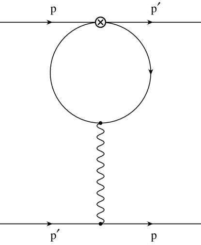
Figure 5: Penguin diagram. We show explicitly the external momenta used in the $RI$ renormalization scheme.

For completeness the matrices $\Delta r^{HV,NDR}_{\lambda^{*}}$, for $\lambda^{*}=0,1$ are given in table 8.

$(i,j)$	$\Delta r^{HV}_{\lambda^{*}=0}$	$\Delta r^{HV}_{\lambda^{*}=1}$	$\Delta r^{NDR}_{\lambda^{*}=0}$	$\Delta r^{NDR}_{\lambda^{*}=1}$
(1,1)	$-7+4{\ln 2}$	$-\frac{37}{6}+\frac{16}{3}{\ln 2}$	$-\frac{7}{3}+4{\ln 2}$	$-\frac{3}{2}+\frac{16}{3}{\ln 2}$
(1,2)	$5-12{\ln 2}$	$\frac{13}{2}-16{\ln 2}$	$7-12{\ln 2}$	$\frac{17}{2}-16{\ln 2}$
(2,1)	$5-12{\ln 2}$	$\frac{13}{2}-16{\ln 2}$	$7-12{\ln 2}$	$\frac{17}{2}-16{\ln 2}$
(2,2)	$-7+4{\ln 2}$	$-\frac{37}{6}+\frac{16}{3}{\ln 2}$	$-\frac{7}{3}+4{\ln 2}$	$-\frac{3}{2}+\frac{16}{3}{\ln 2}$
(2,3)	$-\frac{5}{27}$	$-\frac{5}{27}$	$-\frac{2}{27}$	$-\frac{2}{27}$
(2,4)	$\frac{5}{9}$	$\frac{5}{9}$	$\frac{2}{9}$	$\frac{2}{9}$
(2,5)	$-\frac{5}{27}$	$-\frac{5}{27}$	$-\frac{2}{27}$	$-\frac{2}{27}$
(2,6)	$\frac{5}{9}$	$\frac{5}{9}$	$\frac{2}{9}$	$\frac{2}{9}$
(3,3)	$-\frac{199}{27}+4{\ln 2}$	$-\frac{353}{54}+\frac{16}{3}{\ln 2}$	$-\frac{67}{27}+4{\ln 2}$	$-\frac{89}{54}+\frac{16}{3}{\ln 2}$
(3,4)	$\frac{55}{9}-12{\ln 2}$	$\frac{137}{18}-16{\ln 2}$	$\frac{67}{9}-12{\ln 2}$	$\frac{161}{18}-16{\ln 2}$
(3,5)	$-\frac{10}{27}$	$-\frac{10}{27}$	$-\frac{4}{27}$	$-\frac{4}{27}$
(3,6)	$\frac{10}{9}$	$\frac{10}{9}$	$\frac{4}{9}$	$\frac{4}{9}$
(4,3)	$5-\frac{5f}{27}-12{\ln 2}$	$\frac{13}{2}-\frac{5f}{27}-16{\ln 2}$	$7-\frac{5f}{27}-12{\ln 2}$	$\frac{17}{2}-\frac{5f}{27}-16{\ln 2}$
(4,4)	$-7+\frac{5f}{9}+4{\ln 2}$	$-\frac{37}{6}+\frac{5f}{9}+\frac{16}{3}{\ln 2}$	$-\frac{7}{3}+\frac{5f}{9}+4{\ln 2}$	$-\frac{3}{2}+\frac{5f}{9}+\frac{16}{3}{\ln 2}$
(4,5)	$-\frac{5f}{27}$	$-\frac{5f}{27}$	$-\frac{5f}{27}$	$-\frac{5f}{27}$
(4,6)	$\frac{5f}{9}$	$\frac{5f}{9}$	$\frac{5f}{9}$	$\frac{5f}{9}$
(5,5)	$-\frac{8}{3}+\frac{2}{3}{\ln 2}$	$-\frac{7}{6}+\frac{4}{3}{\ln 2}$	$\frac{2}{3}+\frac{2}{3}{\ln 2}$	$\frac{13}{6}+\frac{4}{3}{\ln 2}$
(5,6)	$-8-2{\ln 2}$	$-\frac{17}{2}-4{\ln 2}$	$-2-2{\ln 2}$	$-\frac{5}{2}-4{\ln 2}$
(6,3)	$-\frac{5f}{27}$	$-\frac{5f}{27}$	$-\frac{5f}{27}$	$-\frac{5f}{27}$
(6,4)	$\frac{5f}{9}$	$\frac{5f}{9}$	$\frac{5f}{9}$	$\frac{5f}{9}$
(6,5)	$-2-\frac{5f}{27}-2{\ln 2}$	$-1-\frac{5f}{27}-4{\ln 2}$	$2-\frac{5f}{27}-2{\ln 2}$	$3-\frac{5f}{27}-4{\ln 2}$
(6,6)	$-\frac{62}{3}+\frac{5f}{9}+\frac{2}{3}{\ln 2}$	$-\frac{71}{3}+\frac{5f}{9}+\frac{4}{3}{\ln 2}$	$-\frac{34}{3}+\frac{5f}{9}+\frac{2}{3}{\ln 2}$	$-\frac{43}{3}+\frac{5f}{9}+\frac{4}{3}{\ln 2}$
(7,7)	$-\frac{8}{3}+\frac{2}{3}{\ln 2}$	$-\frac{7}{6}+\frac{4}{3}{\ln 2}$	$\frac{2}{3}+\frac{2}{3}{\ln 2}$	$\frac{13}{6}+\frac{4}{3}{\ln 2}$
(7,8)	$-8-2{\ln 2}$	$-\frac{17}{2}-4{\ln 2}$	$-2-2{\ln 2}$	$-\frac{5}{2}-4{\ln 2}$
(8,3)	$-\frac{5u}{27}+\frac{5d}{54}$	$-\frac{5u}{27}+\frac{5d}{54}$	$-\frac{5u}{27}+\frac{5d}{54}$	$-\frac{5u}{27}+\frac{5d}{54}$
(8,4)	$\frac{5u}{9}-\frac{5d}{18}$	$\frac{5u}{9}-\frac{5d}{18}$	$\frac{5u}{9}-\frac{5d}{18}$	$\frac{5u}{9}-\frac{5d}{18}$
(8,5)	$-\frac{5u}{27}+\frac{5d}{54}$	$-\frac{5u}{27}+\frac{5d}{54}$	$-\frac{5u}{27}+\frac{5d}{54}$	$-\frac{5u}{27}+\frac{5d}{54}$
(8,6)	$\frac{5u}{9}-\frac{5d}{18}$	$\frac{5u}{9}-\frac{5d}{18}$	$\frac{5u}{9}-\frac{5d}{18}$	$\frac{5u}{9}-\frac{5d}{18}$
(8,7)	$-2-2{\ln 2}$	$-1-4{\ln 2}$	$2-2{\ln 2}$	$3-4{\ln 2}$
(8,8)	$-\frac{62}{3}+\frac{2}{3}{\ln 2}$	$-\frac{71}{3}+\frac{4}{3}{\ln 2}$	$-\frac{34}{3}+\frac{2}{3}{\ln 2}$	$-\frac{43}{3}+\frac{4}{3}{\ln 2}$
(9,3)	$\frac{5}{27}$	$\frac{5}{27}$	$\frac{2}{27}$	$\frac{2}{27}$
(9,4)	$-\frac{5}{9}$	$-\frac{5}{9}$	$-\frac{2}{9}$	$-\frac{2}{9}$
(9,5)	$\frac{5}{27}$	$\frac{5}{27}$	$\frac{2}{27}$	$\frac{2}{27}$
(9,6)	$-\frac{5}{9}$	$-\frac{5}{9}$	$-\frac{2}{9}$	$-\frac{2}{9}$
(9,9)	$-7+4{\ln 2}$	$-\frac{37}{6}+\frac{16}{3}{\ln 2}$	$-\frac{7}{3}+4{\ln 2}$	$-\frac{3}{2}+\frac{16}{3}{\ln 2}$
(9,10)	$5-12{\ln 2}$	$\frac{13}{2}-16{\ln 2}$	$7-12{\ln 2}$	$\frac{17}{2}-16{\ln 2}$

Table 8: The matrices $\Delta r^{HV}_{\lambda^{*}=0,1}$ and $\Delta r^{NDR}_{\lambda^{*}=0,1}$ necessary to relate the Wilson coefficients in the $HV$ and $NDR$ $\overline{MS}$ schemes to those computed in the $RI$ scheme, in the Landau ($\lambda^{*}=0$) and Feynman ($\lambda^{*}=1$) gauges, are given. $(i,j)$ refers to the matrix element. The matrix elements which are zero are not reported. (Continue)

$(i,j)$	$\Delta r^{HV}_{\lambda^{*}=0}$	$\Delta r^{HV}_{\lambda^{*}=1}$	$\Delta r^{NDR}_{\lambda^{*}=0}$	$\Delta r^{NDR}_{\lambda^{*}=1}$
(10,3)	$-\frac{5u}{27}+\frac{5d}{54}$	$-\frac{5u}{27}+\frac{5d}{54}$	$-\frac{5u}{27}+\frac{5d}{54}$	$-\frac{5u}{27}+\frac{5d}{54}$
(10,4)	$\frac{5u}{9}-\frac{5d}{18}$	$\frac{5u}{9}-\frac{5d}{18}$	$\frac{5u}{9}-\frac{5d}{18}$	$\frac{5u}{9}-\frac{5d}{18}$
(10,5)	$-\frac{5u}{27}+\frac{5d}{54}$	$-\frac{5u}{27}+\frac{5d}{54}$	$-\frac{5u}{27}+\frac{5d}{54}$	$-\frac{5u}{27}+\frac{5d}{54}$
(10,6)	$\frac{5u}{9}-\frac{5d}{18}$	$\frac{5u}{9}-\frac{5d}{18}$	$\frac{5u}{9}-\frac{5d}{18}$	$\frac{5u}{9}-\frac{5d}{18}$
(10,9)	$5-12{\ln 2}$	$\frac{13}{2}-16{\ln 2}$	$7-12{\ln 2}$	$\frac{17}{2}-16{\ln 2}$
(10,10)	$-7+4{\ln 2}$	$-\frac{37}{6}+\frac{16}{3}{\ln 2}$	$-\frac{7}{3}+4{\ln 2}$	$-\frac{3}{2}+\frac{16}{3}{\ln 2}$

Table 8: (Continued)

7 $B$-parameters of the relevant operators

Since our last study of $\epsilon^{\prime}/\epsilon$ [11], no significant progress, in lattice calculations of hadronic matrix elements, has been made. We want, however, to discuss a few points not clarified in our previous papers or raised by other authors.

1. In ref. [32], for the kaon $B$-parameter in $NDR$, they found $B_{K}(\mu=2$ GeV$)=0.616\pm 0.020\pm 0.017$. Using this value and the LO conversion factor, they derive the renormalization group-invariant $B_{K}=0.825\pm 0.027\pm 0.023$. For consistency with the present application, since corrections of $O(\alpha_{s})$ were included in the lattice calculation, we have to use the NLO expression (58) instead. In this case, one obtains $B_{K}=0.75$ as central value. We have thus used $B_{K}=0.75$, assuming an error of about $0.15$, because of uncertainties coming from the quenched approximation, the scale in the coupling constant, $\Lambda_{QCD}$, etc.

2. In the absence of electromagnetic corrections, it is possible to demonstrate (non-perturbatively) that

   $$B^{3/2}_{9}(\mu)=B_{K}(\mu)$$

   in any regularization scheme and at any scale $\mu$ . The proof consists in showing that, by assuming $SU(3)$ flavour symmetry, the matrix elements $\langle\pi^{+}\pi^{0}|Q_{9}|K^{+}\rangle_{\Delta I=3/2}$ and $\langle\pi^{+}\pi^{0}|Q^{+}|K^{+}\rangle_{\Delta I=3/2}$ ($Q^{+}=1/2(Q_{1}+Q_{2})$) correspond to the same expression, when written in terms of functional integrals over quark and gluon fields. In the absence of electromagnetic corrections and isospin breaking effects, the same two diagrams as in fig. 6 contribute to both the decay amplitudes.

   

   Figure 6: Diagrams relevant for $B^{3/2}_{9}$ and $(B^{+})^{3/2}$ in the absence of electromagnetic corrections and isospin breaking effects.

   In the presence of $SU(3)$-breaking effects and of the electromagnetic interaction, which has to be included for consistency with the calculation of the Wilson coefficients, $B^{3/2}_{9}$ is, however, different from $(B^{+})^{3/2}$. We are not aware of any non-perturbative estimate of the difference of the $B$-parameters in the presence of the electromagnetic corrections. One may argue that the difference is small, and we have ignored it in our analysis.

3. In ref. [11], we have used the same value of $B^{3/2}_{9}$ as in the present analysis, $B^{3/2}_{9}(\mu=2$ GeV$)=0.62$, see table 3. This value should be compared to $B^{3/2}_{9}(\mu=2$ GeV$)\sim 0.44$, which was used in ref. [15]. Our estimate of $B^{3/2}_{9}$ is derived from the theoretical value of $B_{K}$; in ref. [15], they evaluated $B_{9}^{3/2}$ from the experimental value of $\mbox{Re}\,A_{2}$ instead, by assuming $SU(3)$ symmetry and by neglecting electromagnetic effects. It is well known that, from the $\Delta I=3/2$ amplitude, and using $SU(3)$ flavour symmetry, one obtains a rather low value of the $B_{K}$-parameter, and hence of $B_{9}^{3/2}=B_{K}$. This seems to us the origin of the difference. Given the uncertainties in the extraction of the $B$-parameters, and the electromagnetic and $SU(3)$-breaking effects discussed above, we think that the two different values of $B^{3/2}_{9}$ are both theoretically acceptable.

4. In the absence of a lattice calculation, the values of $B_{1,2}^{c}$ assumed in all our analyses have been guessed taking into account that the corresponding matrix elements vanish in the vacuum insertion approximation. Following ref. [10], we have normalized the matrix elements of $Q_{1,2}^{c}$ to those of $Q_{1,2}^{(1/2)}$ by writing $\langle Q_{1,2}^{c}(\mu)\rangle=B_{1,2}^{c}(\mu)\langle Q_{1,2}^{(1/2)}(\mu)\rangle$. The range of values used by us, given in table 3, has been criticized in ref. [15]. Their argument is the following. By matching at threshold ($\mu=m_{c}$) the effective Hamiltonian, valid for a scale $\mu>m_{c}$, to the effective Hamiltonian, valid for $\mu<m_{c}$, and by assuming the positivity of $\langle O_{\pm}^{c}\rangle$, they demonstrated that $B_{1,2}^{c}(\mu=m_{c})=0$. The values of $B_{1,2}^{c}(\mu>m_{c})$ were then evaluated by using the renormalization group evolution of the corresponding operators; they were found to be much smaller than the upper values used in our case. We believe that this demonstration is not valid because an important point was missed. The effective Hamiltonian, valid for $\mu<m_{c}$, cannot be used to describe the physics at threshold. This is due to the presence of operators of dimension higher than 6, which are usually neglected at $\mu\ll m_{c}$, because their contribution decreases as $(\mu/m_{c})^{k}$, with $k$ a positive integer. Indeed, for $\mu\ll m_{c}$, the effect of these higher dimensional operators enters only in the matching conditions; at threshold, however, all the higher dimensional operators become equally important and their contribution should be included. This turns out to be impossible in practice. For this reason, we believe that our guess for $B_{1,2}^{c}$, although with no theoretical foundation, is an acceptable one.

8 Theoretical uncertainties

In this section we briefly summarize the main sources of uncertainty present in the determination of $\epsilon^{\prime}/\epsilon$. Since many aspects of the calculation have already been discussed in our previous papers on the same subject [8, 11] (see also ref. [15]) we only add here a few considerations that may be useful to the reader.

Theoretical predictions of weak decay amplitudes rely on the perturbative calculation of the Wilson coefficients and on the non-perturbative evaluation of the corresponding matrix elements. Even though the two aspects are intimately connected, we discuss them separately.

8.1 The Wilson coefficients

The main uncertainties in the evaluation of the Wilson coefficients are due to higher order corrections, which will probably remain unknown for a long time, to the value of $\Lambda_{QCD}$, which is taken from experiments, and to the choice of the expansion parameter (i.e. $\alpha_{s}$) and of the renormalization scheme. The latter two are also related to the truncation of the perturbative expansion and can be reduced by increasing the scale $\mu$ at which the operators are renormalized. It should be noticed that the results found in $HV$ and $NDR$, for a top quark mass of $\sim 175$ GeV, differ by about $22\%$. In principle, the differences of the Wilson coefficients in the two different renormalization schemes are compensated, at the NLO, by the corresponding differences in the renormalized operators, and hence in their matrix elements. The matrix $\Delta r$ connecting the two different schemes (cf. sec. 6 and refs. [4]–[8]) has, however, quite large elements. This, combined with the cancellations occurring with a heavy top mass, is at the origin of the sizeable difference (although of $O(\alpha_{s}^{2})$) found between the values of $\epsilon^{\prime}/\epsilon$ in $HV$ and $NDR$.

The larger differences observed in ref. [15] between $HV$ and $NDR$ are due to the fact that the authors changed the coefficient functions without modifying accordingly all the corresponing $B$-parameters, in particular they kept the values of $B_{6}$ and $B_{8}^{3/2}$ fixed.

8.2 Matrix elements

The main limitation to an accurate theoretical prediction of $\epsilon^{\prime}/\epsilon$ does not come, however, from the calculation of the Wilson coefficients, but it is due to the evaluation of the operator matrix elements. We have chosen to work in the framework of lattice $QCD$ for several reasons. Firstly, the matching between the full theory and the effective Hamiltonian can consistently be done at the NLO (or at any higher order). This is not the case of other methods, like for example the $1/N_{c}$-expansion. Secondly, the calculation of the hadronic matrix elements of the relevant operators is based on the fundamental theory without extra-assumptions: there are no free parameters besides the quark masses and the value of the lattice spacing, both of which are fixed by hadron spectroscopy. Thirdly, the typical scale at which the operators are renormalized is of the order of the inverse lattice spacing (see sec. 5), which, in current lattice simulations, is relatively high, $1/a\sim 2$–$4$ GeV. A large renormalization scale, $\mu\sim 1/a$, reduces the systematic error due to the presence of higher-order terms in the matching procedure, as can be seen from the fact that the NLO corrections are smaller at larger values of $\mu$ [11, 15]. Finally, the systematic errors present in lattice calculations (finite volume effects, discretization errors, “quenching”, etc.) can be studied and reduced in time, according to the progress realized with the advent of more powerful computers. In spite of the many advantages offered by the lattice approach, the errors in the theoretical predictions are still rather large. This is due to a variety of reasons:

• Almost all the calculations have so far been done in the so-called “quenched” approximation, which consists in neglecting the effects of the virtual quark loops in the numerical simulation. This approximation is a necessity imposed by the present limitation in computer power. The effects of the quenched approximation on the different physical quantities is not known a priori. In ref. [31], it has been shown that the value of the kaon $B$-parameter $B_{K}$, obtained in a full, “unquenched” $QCD$ calculation with staggered fermions, does not differ appreciably from the corresponding one obtained in the quenched case. It should be noticed, however, that the mass of the quarks at which the calculation of ref. [31] was performed is rather large, thus reducing the effects of the quark loops (the quenched approximation can be obtained by sending to infinity the mass of the quarks in the loops).

• Renormalized lattice operators must correspond, in the limit of infinite lattice cut-off, to finite chiral covariant operators, which obey the same renormalization conditions as in the continuum. With few exceptions, lattice perturbation theory is usually used to evaluate the renormalization constants of lattice operators. The problem of mixing with lower dimensional operators requires, however, a non-perturbative subtraction of all power divergences [54], [58]–[61]. Apart from this special case, the use of perturbation theory, in the computation of multiplicative constants and adimensional mixing coefficients, is well justified, provided that the lattice spacing $a$ is sufficiently small, i.e. $a^{-1}\gg\Lambda_{QCD}$. However, there is evidence of failures of lattice perturbation theory, resulting from the use of the bare lattice coupling constant $\alpha^{{latt}}=g_{0}^{2}/4\pi$, as an expansion parameter. This failure has been attributed to the presence of “tadpole” diagrams, which appear only in the lattice regularization and are likely to give large corrections in higher order perturbation theory. Several solutions to this problem have been proposed so far [53, 55], which could hopefully reduce the systematic error induced by the poor convergence of lattice perturbation theory. It remains to be shown that these methods work in the case of the four-fermion operators relevant for $\epsilon^{\prime}/\epsilon$.

• In most of the lattice simulations, the $\langle\pi|O_{i}|K\rangle$ matrix elements, instead of the more appropriate $\langle\pi\pi|O_{i}|K\rangle$ ones, are indeed computed. The $K\to\pi$ amplitudes are then related to the physical $K\to\pi\pi$ ones using current algebra, at lowest order in the chiral expansion. This certainly introduces an error, which on a single matrix element is probably less than $30\%$. Also in this case, as for the isospin breaking effect mentioned before, the systematic error is amplified by the large cancellations occurring in the final result.

• The crucial $B$-parameter $B_{6}$ has been computed so far (together with $B_{5}$) only by one group [23, 24], using “staggered” lattice fermions. All the attempts to compute $B_{5,6}$ using different lattice formulations of $QCD$, typically using “Wilson fermions”, have failed so far. Morevover, the same techniques applied to a similar problem, the $\Delta I=1/2$ $K\to\pi\pi$ amplitude, were completely unsuccessful. It would be more reassuring to have further confirmations of the values of $B$-parameters computed in refs. [23, 24].

9 Conclusions

In this paper we have discussed several theoretical issues, which are relevant to the prediction of $\epsilon^{\prime}/\epsilon$ and many other weak decays. To our knowledge, the discussion of the matching of the lattice operators to the continuum effective Hamiltonian is new. Sections 5 and 6 contain several useful formulae that can be used in many different applications. With the operator matrix elements from the lattice, one can compute the weak decays amplitudes, using the Wilson coefficients taken from table 4 (5) or 6 (7), with almost no extra effort. The $RI$ renormalization scheme discussed in this paper will become very useful if the non-perturbative method proposed in ref. [53] will succeed in the case of four-fermion operators.

We have also presented an upgraded theoretical analysis of $\epsilon^{\prime}/\epsilon$ in two different renormalization schemes, $NDR$ and $HV$. Let us summarize the main results of the present study. Using the information coming from $\epsilon$ and $x_{d}$, and taking $m_{t}=(174\pm 17)$ GeV and $f_{B}B^{1/2}=(200\pm 40)$ MeV, we obtain constraints on the angles of the unitary triangle

$$\cos\delta=0.47\pm 0.32\,,$$

$$\sin 2\beta=0.65\pm 0.12\,.$$ (64)

Moreover, for $\cos\delta>0$, we predict

$$x_{d}=0.75\pm 0.23\,.$$

Finally, we have obtained

$$\epsilon^{\prime}/\epsilon=(3.1\pm 2.5)\times 10^{-4}$$

as our best estimate. Isospin-breaking effects have been found quite important, because of the large value of $m_{t}$, and we believe that they deserve further theoretical investigation.

References

- [1] F. Abe et al., CDF Collaboration, Phys. Rev. Lett. 73 (1994) 225; Phys. Rev. D50 (1994) 2966.
- [2] G. Barr, Proceedings of the Joint International Lepton-Photon Symposium and Europhysics Conference on HEP, Geneva July 1991, S. Hegardy, K. Potter and E. Quercigh eds., Vol. 1 (1992) p. 179.
- [3] B. Winstein, ibid., p. 186; L.K. Gibbons et al., EFI preprint, EFI 93-06 (1993).
- [4] G. Altarelli, G. Curci, G. Martinelli and S. Petrarca, Nucl. Phys. B187 (1981) 461.
- [5] A.J. Buras, P.H. Weisz, Nucl. Phys. B333 (1990) 66.
- [6] A.J. Buras, M. Jamin, M.E. Lautenbacher and P.H. Weisz, Nucl. Phys. B370 (1992) 69, Addendum, ibid. Nucl Phys. B375 (1992) 501.
- [7] A.J. Buras, M. Jamin and M.E. Lautenbacher, Nucl. Phys. B400 (1993) 37 and B400 (1993) 75.
- [8] M. Ciuchini, E. Franco, G. Martinelli and L. Reina, Nucl. Phys. B415 (1994) 403.
- [9] S. Herrlich and U. Nierste, TUM-T31-49/93 (1993).
- [10] M. Lusignoli, L. Maiani, G. Martinelli and L. Reina, Nucl. Phys. B369 (1992) 139
- [11] M. Ciuchini, E. Franco, G. Martinelli and L. Reina, Phys. Lett. B301 (1993) 263.
- [12] C.R. Allton et al., Nucl. Phys. B431 (1994) 667.
- [13] M. Ciuchini et al., presented by G. Martinelli at the 1st Rencontre du Vietnam, Hanoi (December 1993), to appear in the Proceedings.
- [14] M. Ciuchini et al., presented by M. Ciuchini at International Conference on HEP, Glasgow (July 1994), to appear in the Proceedings.
- [15] A. Buras, M. Jamin and M.E. Lautenbacher, Nucl. Phys. B408 (1993) 209.
- [16] M. Schmidtler and K.R. Schubert, Z. Phys. C53 (1992) 25
- [17] A. Ali and D. London, CERN-TH.7248/94.
- [18] A.J. Buras, W. Slominski and H. Steger, Nucl. Phys. B238 (1984) 529; B245 (1984) 369.
- [19] S. Sharpe, Nucl. Phys. B (Proc. Suppl.) 17 (1990) 146.
- [20] C. Bernard et al., Nucl. Phys. B (Proc. Suppl.) 17 (1990) 495.
- [21] M.B. Gavela et al., Nucl. Phys. B306 (1988) 677.
- [22] G.W. Kilcup et al., Phys. Rev. Lett. 64 (1990) 25.
- [23] G.W. Kilcup, Nucl. Phys. B (Proc. Suppl.) 20 (1991) 417.
- [24] S. Sharpe, Nucl. Phys. B (Proc. Suppl.) 20 (1991) 429.
- [25] G. Martinelli, Phys. Lett. B141 (1984) 395.
- [26] C. Bernard, A. Soni and T. Draper, Phys. Rev. D36 (1987) 3224.
- [27] M.F.L. Golterman and J. Smit, Nucl. Phys. B245 (1984) 61.
- [28] D. Daniel and S. Sheard, Nucl. Phys. B302 (1988) 471.
- [29] S. Sheard, Nucl. Phys. B314 (1989) 238.
- [30] G. Curci, E. Franco, L. Maiani and G. Martinelli, Phys. Lett. B202 (1988) 363.
- [31] N. Ishizuka et al., Phys. Rev. Lett. 71 (1993) 24.
- [32] S. Sharpe, Nucl. Phys. B (Proc. Suppl.) 34 (1994) 403.
- [33] G. ’t Hooft and M. Veltman, Nucl. Phys. B44 (1972) 189.
- [34] C. Becchi et al., Z. Phys. C8 (1981) 335.
- [35] E. de Rafael and S. Narison, Phys. Lett. B103 (1981) 57.
- [36] E. de Rafael et al., Nucl. Phys. B212 (1983) 365.
- [37] C.A. Dominguez and E. de Rafael, Ann. Phys. 174 (1987) 372.
- [38] S. Narison, Phys. Lett. B216 (1991) 1989.
- [39] C.A. Dominguez, C. Van Gend and N. Paver, Phys. Lett. B253 (1991) 241.
- [40] S.G. Gorishny, A.L. Kataev and S.A. Larin, Phys. Lett. B135 (1984) 385; S.G. Gorishny et al., Mod. Phys. Lett. A5 (1990) 2703.
- [41] E. Gabrielli and P. Nason, Phys. Lett. B313 (1993) 430.
- [42] M. Jamin and M. Munz, CERN-TH-7435/94, hep-ph-9409335.
- [43] T. Inami, C.S. Lim, Prog. Theor. Phys. 65 (1981) 297; Erratum 65 (1981) 1772.
- [44] A.J. Buras, M. Jamin and P.H. Weisz, Nucl. Phys. B347 (1990) 491.
- [45] L. Wolfenstein, Phys. Rev. Lett. 51 (1983) 1945.
- [46] M.A. Shifman , A.I. Vainshtein and V.I. Zakharov, Nucl. Phys. B120 (1977) 316; JEPT (Sov. Phys.) 45 (1977) 670.
- [47] F.J. Gilman and M. Wise, Phys. Rev. D27 (1983) 1128.
- [48] J. Bijnens and M. Wise, Phys. Lett. B137 (1984) 245.
- [49] M. Lusignoli, Nucl. Phys. B325 (1989) 33.
- [50] A.J. Buras and J.-M. Gerard, Phys. Lett. B192 (1987) 156.
- [51] J.M. Flynn, L. Randall, Phys. Lett. B224 (1989) 221; Erratum B235 (1990) 412.
- [52] G. Buchalla, A.J. Buras, M.K. Harlander, Nucl. Phys. B337 (1990) 313.
- [53] G. Martinelli et al., presented by C.T. Sachrajda, Nucl. Phys. B (Proc. Suppl.) 34 (1994) 507; CERN-TH 7342/94
- [54] M. Bochicchio et al. Nucl. Phys. B262 (1985) 331.
- [55] G.P. Lepage and P.B. Mackenzie, Nucl. Phys. B (Proc. Suppl) 20 (1991) 173; Phys. Rev. D48 (1993) 2250.
- [56] A. Patel and S. Sharpe, Nucl. Phys. B417 (1994) 307.
- [57] G. Curci and G. Ricciardi, Phys. Rev. D47 (1993) 2991.
- [58] L. Maiani et al., Phys. Lett. B176 (1986) 445; Nucl. Phys. B289 (1987) 505.
- [59] M.B. Gavela et al., Phys. Lett. B211 (1988) 139.
- [60] L. Maiani, G. Martinelli and C.T. Sachrajda, Nucl. Phys. B368 (1992) 281.
- [61] G. Martinelli, Nucl. Phys. B (Proc. Suppl.) 26 (1992) 31.