1 Introduction

Charge symmetry is broken at the most fundamental level in strong interaction physics through the small mass difference between up and down quarks in the QCD Lagrangian. As a consequence the physical $\rho$ and $\omega$ mesons are not eigenstates of isospin but, for example, the physical $\rho$ contains a small admixture of an $I=0$ $q\bar{q}$ state. This phenomenon, known loosely as $\rho\!-\!\omega$ mixing, has been observed in the charge form-factor of the pion, which is dominated by the $\rho$ in the time-like region. Indeed, vector meson dominance (VMD) was constructed to take advantage of this fact.

Nuclear physics involves strongly interacting systems which are not yet amenable to calculations based directly on QCD itself. Instead the nucleon-nucleon (NN) force is often treated in a semi-phenomenological manner using a one- or (two-) boson exchange model. Within such a framework, $\rho\!-\!\omega$ mixing gives rise to a charge symmetry violating (CSV) NN potential which has been remarkably effective in explaining measured CSV in nuclear systems – notably in connection with the Okamoto-Nolen-Schiffer anomaly in mirror nuclei. However, the theoretical consistency of this approach has been challenged by recent work suggesting that the $\rho\!-\!\omega$ mixing amplitude changes sign between the $\rho$ pole and the space-like region involved in the NN interaction.

Our aim is to provide a clear, up-to-date account of the ideas of VMD as they relate particularly to the pion form-factor and to $\rho\!-\!\omega$ mixing. We begin with an historical review of VMD in Sec. 2. The evidence for $\rho\!-\!\omega$ mixing at the $\rho$ pole is presented in Sec. 3 along with the standard theoretical treatment. In Sec. 4 we briefly highlight the role played by $\rho\!-\!\omega$ mixing in the traditional formulation of the CSV NN force. More modern theoretical concerns about the theoretical consistency of the usual approach are summarised in Sec. 5, while in Sec. 6 these new ideas are tested against the form-factor data. In Sec. 7 we make a few remarks concerning shadowing in the light of our new appreciation of VMD, summarise our conclusions and outline some open problems.

2 Vector Meson Dominance

The physics of hadrons was a topic of intense study long before the gauge field theory of quantum chromodynamics (QCD) now believed to describe it completely was invented. Hadronic physics was described using a variety of models and incorporating approximate symmetries. It is a testimony to the insight behind these models (and the inherent difficulties in solving non-perturbative QCD) that they still play an important role in our understanding.

One particularly important aspect of hadronic physics which concerns us here is the interaction between the photon and hadronic matter [1]. This has been remarkably well described using the vector meson dominance (VMD) model. This assumes that the hadronic components of the vacuum polarisation of the photon consist exclusively of the known vector mesons. This is certainly an approximation, but in the regions around the vector meson masses, it appears to be a very good one. As vector mesons are believed to be bound states of quark-antiquark pairs [2, 3, 4], it is tempting to try to establish a connection between the old language of VMD and the Standard Model [5]. In the Standard Model, quarks, being charged, couple to the photon and so the strong sector contribution to the photon propagator arises, in a manner analogous to the electron-positron loops in QED, as shown in Fig. 1.

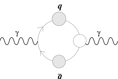
Figure 1: One-particle-irreducible QCD contribution to the photon propagator.

The diagram contains dressed quark propagators and the proper (i.e., one-particle irreducible) photon-quark vertex (the shaded circles include one-particle-reducible parts, while the empty circles are one-particle-irreducible [6]). In QED we can approximate the photon self-energy reasonably well using bare propagators and vertices without worrying about higher-order dressing. However, in QCD, the dressing of these quark loops can not be so readily dismissed as being of higher order in a perturbative expansion. (Although for the heavier quarks, higher order effects can be ignored as a consequence of asymptotic freedom [7], one must be careful about this [8].) No direct translation between the Standard Model and VMD has yet been made.

2.1 Historical development of VMD

The seeds of VMD were sown by Nambu [9] in 1957 when he suggested that the charge distribution of the proton and neutron, as determined by electron scattering, could be accounted for by a heavy neutral vector meson contributing to the nucleon form factor. This isospin-zero field is now called the $\omega$.

The anomalous magnetic moment of the nucleon was believed to be dominated by a two-pion state [10]. The pion form-factor, $F_{\pi}(q^{2})$, (to be discussed later in some detail) was taken to be unity in these initial calculations —i.e., the pions were treated as point-like objects. By 1959 Frazer and Fulco [11] concluded (after an investigation of analytic structure) that the pion form-factor had to satisfy the dispersion relation

$$F_{\pi}(q^{2})=1+\frac{q^{2}}{\pi}\int_{4m_{\pi}^{2}}dr\frac{{\cal I}m\;F_{\pi}(r)}{r(r-q^{2}-i\epsilon)}$$ (1)

and that to be consistent with data a suitable peak in the pion form-factor was required, which they believed could result from a strong pion-pion interaction. The analytic structure of the partial wave amplitude in the physical region could be approximated as a pole of appropriate position and residue (a successful approximation in nucleon-nucleon scattering). An analysis determined that the residue should be positive, raising the possibility of a resonance, which we now know as the $\rho^{0}$.

It was Sakurai who proposed a theory of the strong interaction mediated by vector mesons [12] based on the non-Abelian field theory of Yang and Mills [13]. He was deeply troubled by the problem of the masses of the mesons in such a theory, as they would destroy the local (flavour) gauge invariance. He published his work with this matter unresolved in the hope that it would stimulate further interest in the field.

Kroll, Lee and Zumino did pursue the idea of reproducing VMD from field theory [14]. Within the simplest VMD model the hadronic contribution to the polarisation of the photon takes the form of a propagating vector meson (see Fig. 2). This now replaces the QCD contribution to the polarisation process depicted in Fig. 1.

Figure 2: A simple VMD-picture representation of the hadronic contribution to the photon propagator. The heavier vector mesons are included in generalised VMD models.

This form arises from the assumption that the hadronic electromagnetic current operator, $j_{\mu}^{\rm EM}$, is proportional to the field operators of the vector mesons (multiplied by their mass squared). This is referred to as the the field-current identity. This is then included in the general structure of the hadronic part of the Lagrangian, giving a precise formulation of VMD in terms of a local, Lagrangian field theory. One starts with the identity for the neutral $\rho$-meson

$$[j^{\rm EM}_{\mu}(x)]_{I=1}=\frac{m_{\rho}^{2}}{g_{\rho}}\rho_{\mu}^{0}(x),$$ (2)

and then generalises [15] to an isovector field, ${\vec{\rho}}(x)$, of which $\rho^{0}(x)$ is the third component [i.e., $\rho^{0}(x)\equiv\rho^{3}(x)$]. Eq. (2) implies that the field ${\vec{\rho}}(x)$ is divergenceless under the strong interaction, which is just the usual Proca condition

$$\partial_{\mu}\vec{\rho}^{\;\mu}=0,$$ (3)

for a massive vector field coupling to a conserved current. The resulting Lagrangian for the hadronic sector is the same as the (flavour) Yang-Mills Lagrangian [13], but also has a mass term which destroys the local gauge invariance. Although gauge invariance is necessary for renormalisability, Kroll et al. were unconcerned by this; stating that the non-zero value for the mass made it possible to connect the field conservation equation, Eq. (3), with the equation of motion of the field. The case of a global SU(2) massive vector field (the $\rho$-field) interacting with a triplet pion field and coupled to a conserved current is treated in detail by Lurie [17].

2.2 Gauge invariance and VMD

Sakurai’s analysis of VMD [18, 19] takes place in the context of a local gauge theory. Although a mass term in the Lagrangian breaks gauge symmetry, Sakurai viewed the generation of interactions by minimal substitution in the Lagrangian to be interesting enough to ignore this problem. Lurie [17] has discussed the $\rho,\,\pi,\,N$ system using coupling to conserved currents which reproduces Sakurai’s results. As it only assumes the Lagrangian to be invariant under global SU(2), the appearance of mass terms causes no difficulty. One can then examine how to include the photon in this system. Lurie’s primary concern was to have the $\rho$ couple to a conserved current, and he did this by constructing a Lagrangian whose equation of motion had the Noether current associated with the global SU(2) symmetry appearing on the right hand side. In doing this, he arrives at the standard non-Abelian Lagrangian (given in p. 700 of Ref. [20]), which is where we start.

We begin with the Lagrangian (while Sakurai and Lurie worked in a Euclidean metric, we follow the conventions of Bjorken and Drell [21])

$${\cal L}_{\rm full}=-\frac{1}{4}\vec{\rho}_{\mu\nu}\cdot\vec{\rho}^{\;\mu\nu}+\frac{1}{2}m_{\rho}^{2}\vec{\rho}_{\mu}\cdot\vec{\rho}^{\mu}+\frac{1}{2}D_{\mu}\vec{\pi}\cdot D^{\mu}\vec{\pi}-\frac{1}{2}m_{\pi}^{2}\vec{\pi}\cdot\vec{\pi},$$ (4)

where

$$\vec{\rho}_{\mu\nu}=\partial_{\mu}\vec{\rho}_{\nu}-\partial_{\nu}\vec{\rho}_{\mu}-g\vec{\rho}_{\mu}\times\vec{\rho}_{\nu},$$ (5)

and

$$D_{\mu}\vec{\pi} = (\partial_{\mu}-ig\vec{\rho}_{\mu}\cdot\vec{T})\vec{\pi},$$ (6)

$$= \partial_{\mu}\vec{\pi}-g\vec{\rho}\times\vec{\pi}.$$ (7)

This Lagrangian is symmetric under the transformation

$$\vec{\phi}\rightarrow\vec{\phi}+\vec{\phi}\times\vec{\epsilon},$$ (8)

where $\vec{\phi}$ represents the isovector fields of the $\vec{\rho}$ and $\vec{\pi}$. The generation of interactions from minimal substitution is used by Sakurai and Lurie to motivate universality (i.e., the coupling constant of the $\rho$ introduced via the covariant derivative, $D_{\mu}$, is the same for all particles). However, as a slight violation to this rule is seen experimentally, we shall distinguish between $g$ and the constant $g_{\rho}$ appearing in Eq. (2), which Sakurai equates in order to satisfy a constraint on the pion form-factor (to be discussed later).

From Eq. (7) it follows that

$$\frac{1}{2}D_{\mu}\vec{\pi}\cdot D^{\mu}\vec{\pi}=\frac{1}{2}\partial_{\mu}\vec{\pi}\cdot\partial^{\mu}\vec{\pi}-g\vec{\rho}_{\mu}\cdot(\vec{\pi}\times\partial^{\mu}\vec{\pi})+\frac{1}{2}g^{2}(\vec{\rho}_{\mu}\times\vec{\pi})^{2}.$$ (9)

After some algebra we obtain the equation of motion for the $\rho$ field

$$\partial_{\nu}\vec{\rho}^{\;\nu\mu}+m_{\rho}^{2}\vec{\rho}^{\;\mu}=g\vec{J}^{\mu}_{\rm Noether}$$ (10)

where the Noether current is

$$\vec{J}^{\mu}_{\rm Noether}=-\frac{\partial{\cal L}}{\partial(\partial_{\mu}\vec{\rho}_{\nu})}\times\vec{\rho}_{\nu}-\frac{\partial{\cal L}}{\partial(\partial_{\mu}\vec{\pi})}\times\vec{\pi}$$ (11)

giving

$$\vec{J}^{\mu}_{\rm Noether}=\vec{\rho}^{\;\mu\nu}\times\vec{\rho}_{\nu}+\vec{\pi}\times\partial^{\mu}\vec{\pi}+g(\vec{\rho}^{\;\mu}\times\vec{\pi})\times\vec{\pi}.$$ (12)

As the Noether current is necessarily conserved, Eq. (10) tells us that the field is divergenceless, as in Eq. (3). Transferring the non-Abelian part of the field strength tensor (the cross product in Eq. (5)) to the RHS of Eq. (10) gives us,

$$\partial_{\nu}(\partial^{\nu}\vec{\rho}^{\;\mu}-\partial^{\mu}\vec{\rho}^{\;\nu})+m_{\rho}^{2}\vec{\rho}^{\;\mu}=g(\vec{J}^{\mu}_{\rm Noether}+\partial_{\nu}(\vec{\rho}^{\;\nu}\times\vec{\rho}^{\;\mu})).$$ (13)

Again using the fact that the $\rho$ field is divergenceless (Eq. (3)), we can rewrite the equation of motion in the inverse propagator form

$$(\partial^{2}+m_{\rho}^{2})\vec{\rho}^{\;\mu}=g\vec{J}^{\mu},$$ (14)

where $\vec{J}_{\mu}$ is also a divergenceless current given by

$$\vec{J}^{\mu} = \vec{J}^{\mu}_{\rm Noether}+\partial_{\nu}(\vec{\rho}^{\;\nu}\times\vec{\rho}^{\;\mu})$$ (15)

$$= \vec{J}^{\mu}_{\rm Noether}+\vec{\rho}^{\;\nu}\times\partial_{\nu}\vec{\rho}^{\;\mu}.$$

As Lurie notes, the presence of the $\rho$ field itself in $\vec{J}^{\mu}_{\rm Noether}$ prevents us from writing the interaction part of the Lagrangian in the simple $\vec{\rho}_{\mu}\cdot\vec{J}^{\mu}$ fashion (which is possible for the fermion-vector interaction). A similar situation for scalar electrodynamics is discussed by Itzykson and Zuber [20] (p. 31–33).

Our task now is to include electromagnetism in this model, and to do this we shall allow Eq. (2) to guide us. Eqs. (2) and (14) imply (as $\partial_{\mu}\rightarrow iq_{\mu}$) a corresponding matrix element relation for the electromagnetic interaction

$$\left<B\right|ej^{\rm EM}_{\mu}\left|A\right> = e\left<B\right|\frac{m_{\rho}^{2}}{g_{\rho}}\rho_{\mu}^{3}\left|A\right>$$ (16)

$$= e\frac{m_{\rho}^{2}}{g_{\rho}}\left<B\right|\frac{-gJ_{\mu}^{3}}{q^{2}-m_{\rho}^{2}}\left|A\right>$$

$$= \frac{-iem_{\rho}^{2}}{g_{\rho}}\frac{-i}{q^{2}-m_{\rho}^{2}}\left<B\right|gJ_{\mu}^{3}\left|A\right>.$$ (17)

This is to say that the photon appears to couple to the hadronic field via a $\rho$ meson, to which it couples with strength $em_{\rho}^{2}/g_{\rho}$. (This model is illustrated in Fig. 4b, below.)

Before proceeding, we shall make, as Sakurai does, the simplifying assumption that one can neglect the $\rho$ self-interaction (from now on we shall refer only to the $\rho^{0}\equiv\rho^{3}$), i.e., the parts of the current given by Eq. (15) involving $\rho$ terms, and concern ourselves only with the piece of the current that looks like

$$J^{\mu}_{\pi}=(\vec{\pi}\times\partial^{\mu}\vec{\pi})_{0},$$ (18)

which we shall refer to now simply as $J^{\mu}$. Changing from a Cartesian to a charge basis, we can re-write Eq. (18) as

$$J_{\mu}=i(\pi^{-}\partial_{\mu}\pi^{+}-\pi^{+}\partial_{\mu}\pi^{-}).$$ (19)

As the $\rho^{0}$ decays almost entirely via the two-pion channel, this is a reasonable approximation for the current. We can then write the simple linear coupling term in the Lagrangian, and we shall choose to write $g$ as $g_{\rho\pi\pi}$

$${\cal L}_{\rho\pi}=-g_{\rho\pi\pi}\rho_{\mu}J^{\mu}.$$ (20)

The important problem now is to ensure that after adding electromagnetism we still have a gauge invariant theory. The naive $\gamma\!-\!\rho$ vertex prescription usually seen in discussions of VMD,

$$-\frac{em_{\rho}^{2}}{g_{\rho}},$$

as motivated by Eq. (17), suggests a coupling term in the effective Lagrangian of the form

$${\cal L}_{\rm eff}=-\frac{em_{\rho}^{2}}{g_{\rho}}\rho^{3}_{\mu}A^{\mu}.$$ (21)

This is suggested by the substitution of the field current identity (Eq. (2)) into the interaction piece of the electromagnetic Lagrangian, $-ej^{\rm EM}_{\mu}A^{\mu}$. However electromagnetism cannot be incorporated into Eq. (4) simply by adding Eq. (21) and a kinetic term for the photon. This would result in the photon acquiring an imaginary mass [12] when one considers the dressing of the photon propagator in the manner of Fig. 3 using $\rho-\gamma$ vertices determined by Eq. (21).

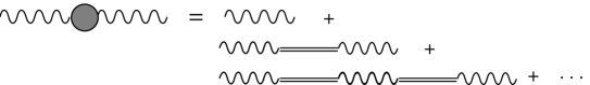
Figure 3: VMD dressing of the photon propagator by a series of intermediate $\rho$ propagators.

However, we can find a term that emulates Eq. (21), but ensures that the photon remains massless. Such a term is

$${\cal L}_{\gamma\rho}=-\frac{e}{2g_{\rho}}F_{\mu\nu}\rho^{\mu\nu}.$$ (22)

We need to re-express this in momentum space which can be done using integration by parts to transform $\partial_{\mu}A_{\nu}\partial^{\mu}\rho^{\nu}$ to $-\partial_{\mu}\partial^{\mu}A_{\nu}\rho^{\nu}$ and then send $\partial_{\mu}\rightarrow iq_{\mu}$ giving

$$F_{\mu\nu}\rho^{\mu\nu}\rightarrow 2q^{2}A_{\mu}\rho^{\mu}.$$ (23)

The other term in $F_{\mu\nu}\rho^{\mu\nu}$ can be discarded because it contains a piece that can be written as $q_{\mu}\rho^{\mu}$ and thus vanishes as the $\rho$ field is divergenceless.

However, the interaction Lagrangian of Eq. (22) is not sufficient as it would decouple the photon from the $\rho$ (and hence then from hadronic matter) at $q^{2}=0$. What is needed is another term which directly couples the photon to hadronic matter. This is

$$-eA_{\mu}J^{\mu},$$ (24)

where $J_{\mu}$ is the hadronic current to which the $\rho$ couples, the pion component of which is given in Eq. (18). Thus we have an interaction between the photon and hadronic matter of exactly the same form as that between the $\rho$ and hadronic matter (though suppressed by a factor of $e/g_{\rho\pi\pi}$). This term is most noticeable at $q^{2}=0$ where the influence of the $\rho$-meson in the photon-pion interaction vanishes.

To summarise the arguments just given, the photon and vector meson part of the Lagrangian we require is

$${\cal L}_{\rm VMD1}=-\frac{1}{4}F_{\mu\nu}F^{\mu\nu}-\frac{1}{4}\rho_{\mu\nu}\rho^{\mu\nu}+\frac{1}{2}m_{\rho}^{2}\rho_{\mu}\rho^{\mu}-g_{\rho\pi\pi}\rho_{\mu}J^{\mu}-eA_{\mu}J^{\mu}-\frac{e}{2g_{\rho}}F_{\mu\nu}\rho^{\mu\nu}.$$ (25)

We shall refer to this as the first representation of VMD. We note that this representation has a direct photon—matter coupling as well as a photon—$\rho$ coupling which vanishes at $q^{2}=0$.

Sakurai also outlined an alternative formulation of VMD, which has survived to become the standard representation. In many ways it is not as elegant as the first; for instance, the Lagrangian has a photon mass term. Despite this it has established itself as the most popular representation of VMD:

$${\cal L}_{\rm VMD2}=-\frac{1}{4}(F^{\prime}_{\mu\nu})^{2}-\frac{1}{4}(\rho^{\prime}_{\mu\nu})^{2}+\frac{1}{2}m_{\rho}^{2}(\rho^{\prime}_{\mu})^{2}-g_{\rho\pi\pi}\rho^{\prime}_{\mu}J^{\mu}-\frac{e^{\prime}m_{\rho}^{2}}{g_{\rho}}\rho^{\prime}_{\mu}A^{\prime\mu}+\frac{1}{2}\left(\frac{e^{\prime}}{g_{\rho}}\right)^{2}m_{\rho}^{2}(A^{\prime}_{\mu})^{2}.$$ (26)

In the limit of universality ($g_{\rho}\!=\!g_{\rho\pi\pi}$) the two representations become equivalent and one can transform between them using

$$\rho^{\prime}_{\mu} = \rho_{\mu}+\frac{e}{g_{\rho}}A_{\mu},$$ (27)

$$A^{\prime}_{\mu} = A_{\mu}\sqrt{1-\left(\frac{e}{g_{\rho}}\right)^{2}},$$ (28)

$$e^{\prime} = e\sqrt{1-\left(\frac{e}{g_{\rho}}\right)^{2}}.$$ (29)

Substituting for $\rho^{\prime}_{\mu},A^{\prime}_{\mu}$ and $e^{\prime}$ in Eq. (26) gives Eq. (25) $+O((e/g_{\rho})^{3})$. We shall refer to Eq. (26) as the second representation of VMD.

The appearance of a photon mass term at first seems slightly troublesome. However, when dressing the photon in the manner of Fig. 3, we see that the propagator has the correct form as $q^{2}\rightarrow 0$. We have

$$iD(q^{2})=\frac{-i}{q^{2}-\frac{e^{2}m_{\rho}^{2}}{g_{\rho}^{2}}}+\frac{-i}{q^{2}-\frac{e^{2}m_{\rho}^{2}}{g_{\rho}^{2}}}\frac{-iem_{\rho}^{2}}{g_{\rho}}\frac{-i}{q^{2}-m_{\rho}^{2}}\frac{-iem_{\rho}^{2}}{g_{\rho}}\frac{-i}{q^{2}-\frac{e^{2}m_{\rho}^{2}}{g_{\rho}^{2}}}+\cdots$$ (30)

Summing this using the general operator identity

$$\frac{1}{A-B}=\frac{1}{A}+\frac{1}{A}B\frac{1}{A}+\frac{1}{A}B\frac{1}{A}B\frac{1}{A}+\cdots$$ (31)

we obtain ($m\equiv m_{\rho}$)

$$iD(q^{2}) = -i\left[q^{2}-\frac{e^{2}m^{2}}{g_{\rho}^{2}}-\frac{e^{2}m^{4}}{g_{\rho}^{2}(q^{2}-m^{2})}\right]^{-1}$$ (32)

$$= -i\left[q^{2}-\frac{e^{2}m^{2}}{g_{\rho}^{2}}+\right.\left.\frac{e^{2}m^{2}}{g_{\rho}^{2}(1-{q^{2}}/{m^{2}})}\right]^{-1}$$

$$\rightarrow \frac{-i}{q^{2}(1+e^{2}/g_{\rho}^{2})}$$ (33)

as $q^{2}\rightarrow 0$. We are thus left with a modification to the coupling constant

$$e^{2}\rightarrow e^{2}(1-e^{2}/g^{2}_{\rho}),$$ (34)

and interestingly we see that the photon propagator is significantly modified away from $q^{2}=0$.

We conclude this discussion with a comparison of the use of the two models by describing the process $\gamma\rightarrow\pi^{+}\pi^{-}$. We can identify the relevant terms in the Lagrangian for each case. From ${\cal L}_{\rm VMD1}$ (Eq. (25)) and ${\cal L}_{\rm VMD2}$ (Eq. (26)) we have, respectively,

$${\cal L}_{1} = -\frac{e}{2g_{\rho}}F_{\mu\nu}\rho^{\mu\nu}-eJ_{\mu}A^{\mu}-g_{\rho\pi\pi}\rho^{\mu}J_{\mu},$$ (35)

$${\cal L}_{2} = -\frac{em_{\rho}^{2}}{g_{\rho}}\rho_{\mu}A^{\mu}-g_{\rho\pi\pi}\rho_{\mu}J^{\mu}.$$ (36)

If the photon coupled to the pions directly, then the Feynman amplitude for this process would be (as in scalar electrodynamics [20])

$${\cal M}^{\mu}_{\gamma\rightarrow\pi^{+}\pi^{-}}=\langle\pi^{+}\pi^{-}|eJ^{\mu}|0\rangle=-e(p^{+}-p^{-})^{\mu},$$ (37)

Where $J_{\mu}$ is given in Eq. (19). However, in the presence of the vector meson interactions of Eqs. (35) and (36), the total amplitude is modified. The pion form factor, $F_{\pi}(q^{2})$, which represents the contribution from the intermediate steps connecting the photon to the pions, is defined by the relation

$${\cal M}^{\mu}_{\gamma\rightarrow\pi^{+}\pi^{-}}=-e(p^{+}-p^{-})^{\mu}F_{\pi}(q^{2}),$$ (38)

where now ${\cal M}^{\mu}_{\gamma\rightarrow\pi^{+}\pi^{-}}$ is the full amplitude including all possible processes. The form-factor is the multiplicative deviation from a pointlike behaviour of the coupling of the photon to the pion field. We discuss $F_{\pi}(q^{2})$ in detail later.

To lowest order, we have for ${\cal L}_{1}$ (see Eq. (23))

$$F_{\pi}(q^{2})=\left[1-\frac{q^{2}}{q^{2}-m_{\rho}^{2}}\frac{g_{\rho\pi\pi}}{g_{\rho}}\right],$$ (39)

and for ${\cal L}_{2}$

$$F_{\pi}(q^{2})=-\frac{m_{\rho}^{2}}{q^{2}-m_{\rho}^{2}}\frac{g_{\rho\pi\pi}}{g_{\rho}}.$$ (40)

In the limit of zero momentum transfer, the photon “sees” only the charge of the pions, and hence we must have

$$F_{\pi}(0)=1.$$ (41)

The reader may notice that Eq. (41) is automatically satisfied by the dispersion relation of Frazer and Fulco, Eq. (1) and by VMD1 (Eq. (39)) but must be imposed on the VMD2 result (Eq. (40)) by demanding $g_{\rho\pi\pi}=g_{\rho}$.

This is the basis of Sakurai’s argument for universality mentioned earlier, i.e., that the photon couples to the $\rho$ as in Eq. (36) and that therefore $g_{\rho\pi\pi}$ must equal $g_{\rho}$. This is a direct consequence of assuming complete $\rho$ dominance of the form-factor (i.e., VMD2). The second part of universality, namely that $g_{\rho\pi\pi}=g_{\rho NN}=...=g_{\rho}$ results from the assumption that the interactions are all generated from the gauge principle (i.e., by minimal substitution for the covariant derivative given in Eq. (6)).

As Sakurai points out, the two representations of VMD are equivalent in the limit of universality (as we would expect from Eqs. (27–29)). Without universality only VMD1, maintains the condition $F_{\pi}(0)=1$. Due to the popularity of the second interpretation, though, $F_{\pi}(0)=1$ is more often viewed as a constraint on various introduced parameters [22]. We illustrate the difference between the two representations in Fig. 4.

Figure 4: Contributions to the pion form-factor in the two representations of vector meson dominance a) VMD1 b) VMD2.

Interestingly, Caldi and Pagels [23] arrived at a similar expression for the pion form-factor to Eq. (39) from a direct photon contribution and a fixed $\gamma\!-\!\rho$ vertex. Their coupling of the $\rho$ to the pion field, though, is momentum dependent, and it is because of this that they reproduced the first representation.

2.3 The $\rho$ as a dynamical gauge boson

Bando et al. have succeeded in constructing a local gauge model which reproduces VMD [24]. This model is based on the idea of a hidden local symmetry originally developed in supergravity theories. The $\rho$-meson appears as the dynamical gauge boson of a hidden local symmetry in the non-linear, chiral Lagrangian. The mass of the $\rho$ is generated by the Higgs mechanism associated with the hidden local symmetry.

We begin with the Lagrangian of the non-linear sigma-model [25]

$${\cal L}=\frac{f_{\pi}^{2}}{4}{\rm Tr}[\partial_{\mu}U\partial^{\mu}U^{\dagger}],$$ (42)

where $f_{\pi}$ is the pion decay constant (93 MeV) and

$$U(x)=\exp[2i\pi(x)/f_{\pi}].$$ (43)

Here $\pi(x)$ are the pion fields $\pi(x)=\pi^{a}T^{a}$, where $T^{a}$ are the generators of SU(2) (see footnote 2 on page 2). The field $U$ transforms under chiral ${\rm SU}(2)_{L}\otimes{\rm SU}(2)_{R}$ as:

$$U(x)\rightarrow g_{L}U(x)g^{\dagger}_{R},$$ (44)

where $g_{L,R}\in{\rm SU}(2)_{L,R}.$

As it stands this particular Lagrangian is invariant under global ${\rm SU}(2)_{L}\otimes{\rm SU}(2)_{R}$. However, it can be cast into a form which possesses, in addition, a local (and hidden) ${\rm SU}(2)_{V}$ symmetry. We can separate $U(x)$ into two constituents which transform respectively under left and right ${\rm SU}(2)$

$$U(x)\equiv\xi_{L}^{\dagger}(x)\xi_{R}(x)$$ (45)

where the $\xi(x)$ are SU(2) matrix-valued entities transforming like

$$\xi_{L,R}\rightarrow\xi_{L,R}g^{\dagger}_{L,R}.$$ (46)

However, the interesting part comes in supposing these components also possess a local ${\rm SU}(2)_{V}$ symmetry,

$$\xi_{L,R}\rightarrow h(x)\xi_{L,R},$$ (47)

where $h(x)=e^{-i\vec{\alpha}(x)\cdot\vec{T}}$. The important point here is that the field $U(x)$ does not “see” this local ${\rm SU}(2)_{V}$ transformation (because it is invariant under it, even though its components $\xi$ are not), and thus we say it is a hidden symmetry.

The ${\rm SU}(2)_{V}$ invariant Lagrangian can now be re-written [25] as

$${\cal L}=f^{2}_{\pi}{\rm Tr}\left[\frac{1}{2i}(\partial_{\mu}\xi_{L}\xi^{\dagger}_{L}-\partial_{\mu}\xi_{R}\xi_{R}^{\dagger})\right]^{2}.$$ (48)

However, if we now introduce a gauge field

$$V_{\mu}=\vec{V}_{\mu}\cdot\vec{T},$$

and covariant derivative (c.f. Eq. (7))

$$D_{\mu}\xi_{L,R}=\partial_{\mu}\xi_{L,R}-igV_{\mu}\xi_{L,R}.$$ (49)

We can write the original Lagrangian as [25]

$${\cal L}_{1}=f^{2}_{\pi}{\rm Tr}\left[\frac{1}{2i}(D_{\mu}\xi_{L}\xi^{\dagger}_{L}-D_{\mu}\xi_{R}\xi_{R}^{\dagger})\right]^{2},$$ (50)

which is easily seen to revert to Eq. (48) upon substitution for the covariant derivatives. We now similarly construct

$${\cal L}_{2} = f^{2}_{\pi}{\rm Tr}\left[\frac{1}{2i}(D_{\mu}\xi_{L}\xi^{\dagger}_{L}+D_{\mu}\xi_{R}\xi_{R}^{\dagger})\right]^{2}$$ (51)

$$= g^{2}f^{2}_{\pi}{\rm Tr}\left[V_{\mu}-\frac{1}{2ig}(\partial_{\mu}\xi_{L}\xi^{\dagger}_{L}+\partial_{\mu}\xi_{R}\xi_{R}^{\dagger})\right]^{2}$$ (52)

which is invariant under the local ${\rm SU}(2)_{V}$ transformation $h(x)$ provided that $V_{\mu}$ transforms under ${\rm SU}(2)_{V}$ as

$$V\rightarrow h(x)Vh^{\dagger}(x)+\frac{i}{g}\;h(x)\partial_{\mu}h^{\dagger}(x).$$ (53)

Interestingly, the Euler-Lagrange equation for $V_{\mu}$ is

$$\frac{\partial{\cal L}}{\partial V_{\mu}}-\partial_{\nu}\left(\right.\frac{\partial{\cal L}}{\partial(\partial_{\nu}V_{\mu})}\left.\right)=0,$$ (54)

which implies that ${\cal L}_{2}=0$. Thus we need to do something to enable us to keep our vector field, $V_{\mu}(x)$. Bando et al. assumed that quantum (or dynamical) effects at the “composite level” (where the underlying quark substructure brings QCD into play) generate the kinetic term of the gauge field $V_{\mu}(x)$

$$-\frac{1}{4}\vec{F}_{\mu\nu}\cdot\vec{F}^{\mu\nu}$$

where, like $\vec{\rho}^{\;\mu\nu}$ in Eq. (5),

$$\vec{F}_{\mu\nu}=\partial_{\mu}\vec{V}_{\nu}-\partial_{\nu}\vec{V}_{\mu}-g\vec{V}_{\mu}\times\vec{V}_{\nu}.$$ (55)

From this we construct a new Lagrangian of the form

$${\cal L}={\cal L}_{1}+a{\cal L}_{2}-\frac{1}{4}\vec{F}_{\mu\nu}\cdot\vec{F}^{\mu\nu},$$ (56)

where $a$ is an arbitrary parameter. We now fix the ${\rm SU}(2)_{V}$ gauge (Eq. (47)) by imposing the condition

$$\xi_{L}^{\dagger}(x)=\xi_{R}(x)=\xi(x)=e^{i\vec{\pi}(x)\cdot\vec{T}/f_{\pi}}.$$ (57)

Approximating $\xi$ by $(1+i\vec{\pi}\cdot\vec{T}/f_{\pi})$ our Lagrangian now has the form

$${\cal L}=\frac{f_{\pi}^{2}}{4}{\rm Tr}[\partial_{\mu}U\partial^{\mu}U^{\dagger}]+\frac{1}{2}ag^{2}f_{\pi}^{2}\vec{V}_{\mu}\cdot\vec{V}^{\mu}-\frac{1}{2}ag\vec{V}\cdot\vec{\pi}\times\partial_{\mu}\vec{\pi}-\frac{1}{4}\vec{F}_{\mu\nu}\cdot\vec{F}^{\mu\nu},$$ (58)

to order $\pi^{2}$. We can identify, by comparison with Eq. (4),

$$m_{\rho}^{2}=ag^{2}f_{\pi}^{2},$$ (59)

and from Eq. (12) we recognise the current

$$\vec{J}^{V}_{\mu}=\vec{\pi}\times\partial_{\mu}\vec{\pi},$$ (60)

and hence,

$$g_{V\pi\pi}=\frac{1}{2}ag.$$ (61)

The next step towards reproducing VMD is to incorporate electromagnetism. We extend the hidden gauge group to a larger group, ${\rm SU}(2)_{V}\otimes{\rm U}(1)_{Q}$ where ${\rm U}(1)_{Q}$ is not a hidden symmetry as

$$U\rightarrow b(x)Ub^{\dagger}(x).$$ (62)

The transformation $b(x)\in{\rm U}(1)_{Q}=\exp(-ie_{0}Q\theta(x))$, where $Q$ is the generator of the one-parameter U(1) group (analogous to $T^{a}$ for SU($N$)). The EM field couples to

$$Q=\frac{1}{2}Y+T_{3},$$ (63)

where $Y$ is the hypercharge, which is zero in this case. Bando et al. draw attention to the complete independence of the $\rho$ and photon source charges, which produces a simple picture.

The transformation given in Eq. (62) means that the $\xi$ fields transform like

$$\xi_{L,R}\rightarrow\xi_{L,R}b^{\dagger}.$$ (64)

We therefore require for a covariant derivative,

$$D_{\mu}\xi_{L,R}=\partial_{\mu}\xi_{L,R}-ig\vec{V}_{\mu}\vec{T}\xi_{L,R}-ie_{0}\xi_{L,R}B_{\mu}T^{3},$$ (65)

where $B_{\mu}$ is essentially the photon field. With this we find that the relevant parts of the Lagrangian, namely

$$D_{\mu}\xi_{L}\xi_{L}^{\dagger}\pm D_{\mu}\xi_{R}\xi_{R}^{\dagger}$$

are invariant under ${\rm U(1)_{Q}}$, provided $B_{\mu}$ transforms like

$$B_{\mu}\rightarrow B_{\mu}-\frac{i}{e_{0}}\;\partial_{\mu}b^{\dagger}b.$$ (66)

Incorporating our new covariant derivative (Eq. (65)) we have as the new Lagrangian

$${\cal L}={\cal L}_{1}+a{\cal L}_{2}-\frac{1}{4}\vec{F}_{\mu\nu}\cdot\vec{F}^{\mu\nu}-\frac{1}{4}B_{\mu\nu}B^{\mu\nu},$$ (67)

where $B_{\mu\nu}$ is the strength tensor of the field $B_{\mu}$. We now once again fix the gauge in the manner of Eq. (57).

Expanding $\xi$ once again to first order in $\vec{\pi}$, the new Lagrangian becomes

$${\cal L}={\frac{f_{\pi}^{2}}{4}}{\rm Tr}[\partial_{\mu}U\partial^{\mu}U^{\dagger}]-{\frac{1}{4}}\vec{F}_{\mu\nu}\cdot\vec{F}^{\mu\nu}-{\frac{1}{4}}(\partial_{\mu}B_{\nu}-\partial_{\nu}B_{\mu})^{2}$$

$$+{\frac{1}{2}}m_{\rho}^{2}\vec{V}_{\mu}\cdot\vec{V}^{\mu}-{\frac{1}{g}}e_{0}m_{\rho}^{2}V_{\mu}^{3}B^{\mu}+{\frac{1}{2}}(\frac{e_{0}}{g})^{2}m_{\rho}^{2}B^{\mu}B_{\mu}$$

$$-{\frac{1}{2}}ag\vec{V}_{\mu}\cdot(\partial^{\mu}\vec{\pi}\times\vec{\pi})-e_{0}(1-{\frac{a}{2}})B^{\mu}(\partial^{\mu}\vec{\pi}\times\vec{\pi})_{3}.$$ (68)

We are now free to choose a value for $a$. Choosing $a=2$ both reproduces the VMD2 Lagrangian given in Eq. (26) and imposes universality as $g_{\rho\pi\pi}=ag/2=g_{\rho}$. One would then be free to make the transformations given by Eq. (29) to obtain VMD1 (Eq. (25)).

However, instead of doing this Bando et al. follow the procedure for removing the mass of the U(1) field in the Standard Model [5], where an almost identical situation occurs for the photon and the $Z^{0}$. One says that the states $V_{3}^{\mu}$ and $B^{\mu}$ mix, spontaneously breaking the ${\rm SU}(2)_{V}\otimes{\rm U}(1)_{Q}$ down to ${\rm U}(1)_{\rm em}$. We set, as opposed to Eqs. (27)-(29),

$$A_{\mu}=\frac{1}{\sqrt{g^{2}+e_{0}^{2}}}(gB_{\mu}+e_{0}V^{3}_{\mu})$$ (69)

$$V^{0}_{\mu}=\frac{1}{\sqrt{g^{2}+e_{0}^{2}}}(gV^{3}_{\mu}-e_{0}B_{\mu})$$ (70)

and the photon mass vanishes as required. The relevant part of the resulting Lagrangian is now

$${\cal L}=-\frac{1}{4}(A_{\mu\nu}A^{\mu\nu}+V^{0}_{\mu\nu}V^{0{\mu\nu}})+\frac{1}{2}(m_{\rho^{0}})^{2}V^{0}_{\mu}V^{0\mu}-(g_{\rho\pi\pi}V^{0}_{\mu}+eA_{\mu})\epsilon_{3ab}\partial^{\mu}\pi^{a}\pi^{b},$$ (71)

where

$$m_{\rho^{0}}^{2} = a(g^{2}+e_{0}^{2})f_{\pi}^{2},$$

$$e = \frac{e_{0}g}{\sqrt{g^{2}+e_{0}^{2}}},$$

$$g_{\rho\pi\pi} = \frac{ge}{e_{0}},$$

for $a\!=\!2$.

We note that this Lagrangian has no explicit coupling between the photon and the $\rho^{0}$, although there is a direct coupling of the photon to the hadronic current. They can mix, however, via a pion-loop, which results in a $q^{2}$ dependent mixing between the photon and the $\rho$-meson. Because we are working to lowest order in the pion field Eq. (71) lacks the seagull term (i.e., one of the form of the final term in Eq. (9)) the resulting mixing amplitude will be neither transverse, nor vanish at $q^{2}=0$ (see section 5.1). However, this is a departure from the usual formulations of VMD which contain an explicit mixing term in the Lagrangian. Bhaduri merely notes that once this transformation is made the physical photon now has a hadron-like part through Eq. (70) [25]. This issue is analysed in more detail by Schechter [26]. He considers the diagonal basis to be the physical one (as the photon is massless and gauge invariance is preserved) and argues that the vector meson supplies a $q^{2}$ correction to the pion form factor, rather than giving the whole thing.

Hung has extended this model to include the weak bosons [27]. What is especially interesting about his work in light of our presentation is his reproduction of the first representation of VMD, which he demonstrates is equivalent to “precisely the old vector meson dominance” (by which he means the second representation), as universality is a consequence of his model.

2.4 Summary

We have described how the interactions of the photon with hadronic systems can be usefully modelled using vector mesons. This idea was then moulded into a Lagrangian field theory, but the masses of the vector meson prevented one from having a gauge invariant theory. Two equivalent formulations of VMD were developed, VMD1 in which the coupling of the photon to the $\rho$ is momentum dependent (vanishing at $q^{2}=0$), and VMD2 where it is not. If universality is imposed these representations produce the same physics.

In an attempt to put VMD on a more solid theoretical footing, Bando et al. were able to write down a gauge invariant theory which reduces (c.f. Eq. (68)) to the VMD2 Lagrangian when one expands to second order in the pion field.

A unified picture of these above mentioned phenomenological approaches is afforded by the bosonised Nambu–Jona-Lasinio (NJL) model [28]. The NJL model features a four-point quark interaction. Bosonising this chirally invariant model automatically yields the field current identity of Eq. (2) and, from this, VMD. The bosonised NJL model also contains the hidden local symmetry of Bando et al. and one can demonstrate, through a chiral rotation, that the two effective meson Lagrangians are equivalent. In the full quantum theory, the two representations, VMD1 and VMD2 are related by a simple change of mesonic integration variables [29].

3 $\rho\!-\!\omega$ mixing

We shall discuss here how $\rho\!-\!\omega$ mixing was seen experimentally and the challenge it presented to physicists to explain the mechanism driving it. The importance of $\rho\!-\!\omega$ mixing in the conventional understanding of charge symmetry violation (CSV) in nuclear physics (c.f. Sec. 4) has made it crucial for us to improve our understanding of this phenomenon.

3.1 The electromagnetic form-factor of the pion

One problem in which VMD found particular success was the description of the electromagnetic form-factor of the pion [30]. As this has played such a crucial role in our understanding of $\rho\!-\!\omega$ mixing it is useful to outline what we mean by it and how the theoretical predictions are compared with experimental data.

We are concerned with the $s$-channel process depicted in Fig. 5, in which an electron-positron pair annihilate, forming a photon which then decays to two pions.

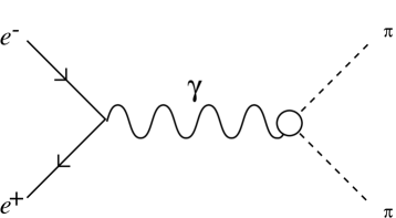
Figure 5: Electron-positron pair annihilating to form a photon which then decays to a pion pair.

We define the form-factor, $F_{\pi}(s)$, by Eq. (38). The form-factor represents all possible strong interactions occurring within the circle in Fig. 5, which we model using VMD.

In the time-like region, $F_{\pi}(q^{2})$ is measured experimentally in the process $e^{+}e^{-}\rightarrow\pi^{+}\pi^{-}$, which, to lowest order in $e^{2}$, is given by the process shown in Fig. 5. The momenta of the electron and positron are $p_{1}$ and $p_{2}$ respectively, and $p_{3}$ and $p_{4}$ are the momenta of the $\pi^{+}$ and $\pi^{-}$. The differential cross-section is given by

$$\frac{d\sigma}{d\Omega}=\frac{\vec{p}_{3}^{\;2}}{|\vec{p}_{3}|(p^{0}_{3}+p^{0}_{4})-p^{0}_{3}\hat{p}_{2}\cdot(\vec{p}_{1}+\vec{p}_{2})}\frac{\frac{1}{4}\Sigma_{\rm pols}|{\cal M}_{fi}|^{2}}{64\pi^{2}\sqrt{(p_{1}\cdot p_{2})^{2}-m_{e}^{4}}},$$ (72)

where $\hat{p}$ is the unit vector in the direction of $\vec{p}$. We are thus interested in calculating the Feynman amplitude, ${\cal M}_{fi}$, for this process. The leptonic and photon part of the diagram are completely standard. The interesting part of the diagram concerns the coupling of the photon to the pion pair represented by Fig. 5. The form of this part of the diagram, ${\cal M}_{\gamma\rightarrow\pi^{+}\pi^{-}}$, is given in Eq. (38). In full, the amplitude is

$${\cal M}_{fi}=\overline{v}(2)ie\gamma^{\mu}u(1)iD_{\mu\nu}(q)eF_{\pi}(q^{2})(p_{4}-p_{3})^{\nu},$$ (73)

with the photon propagator being given by

$$iD_{\mu\nu}(q)=\frac{(-i)}{q^{2}}\left[g_{\mu\nu}+(\xi-1)\frac{q_{\mu}q_{\nu}}{q^{2}}\right].$$ (74)

Particular choices of $\xi$ correspond to particular covariant gauges. The second term in Eq. (74) vanishes because the phton couples to conserved currents.

In the centre of mass frame in which we set $|\vec{p}|=p$, we have $E^{2}-p^{2}=m_{e}^{2}$, $E^{2}-p^{\prime 2}=m_{\pi}^{2}$, and $\vec{p}\cdot\vec{p}\;^{\prime}=-pp^{\prime}\cos\theta$. Using $\sqrt{s}=2E$ the differential cross-section becomes

$$\frac{d\sigma}{d\Omega}=\frac{e^{4}}{s^{2}}\frac{(\frac{1}{4}s-m_{\pi}^{2})^{1/2}}{(\frac{1}{4}s^{2}-sm_{e}^{2})^{1/2}}\frac{(E^{4}-E^{2}m_{\pi}^{2}-((E^{4}-E^{2}(m_{\pi}^{2}+m_{e}^{2})+m_{\pi}^{2}m_{e}^{2})\cos^{2}\theta))|F_{\pi}(s)|^{2}}{\sqrt{s}\;64\pi^{2}}.$$ (75)

Since we have $m_{e}^{2}<<m_{\pi}^{2}<s$, we can simplify the above formula to

$$\frac{d\sigma}{d\Omega}=\frac{e^{4}}{s^{2}}\frac{(s-4m_{\pi}^{2})^{1/2}}{s\sqrt{s}}\frac{1}{8\pi^{2}}(E^{4}-E^{2}m_{\pi}^{2})(1-\cos^{2}\theta)|F_{\pi}(s)|^{2}.$$

From this we obtain the total cross-section

$$\sigma=\frac{\alpha^{2}\pi}{3}\frac{(s-4m_{\pi}^{2})^{3/2}}{s^{5/2}}|F_{\pi}(s)|^{2}.$$ (76)

Early experiments measuring this cross-section produced enough data around the $\rho$ resonance to enable the extraction of $|F_{\pi}(s)|^{2}$ and led to the development of the VMD model discussed earlier. In the second representation of VMD the $e^{+}e^{-}\rightarrow\pi^{+}\pi^{-}$ reaction is given by the process illustrated in Fig. 6, which leads to the expression for the pion form-factor, as given in Eq. (40),

$$F_{\pi}(s)=\frac{-m_{\rho}^{2}}{s-m_{\rho}^{2}+im_{\rho}\Gamma_{\rho}}.$$ (77)

The reader will notice Eq. (77) differs slightly from what would be naively expected from Eq. (40) as the width of the $\rho$-meson has been included. This will be fully discussed later.

Figure 6: VMD description of $e^{+}e^{-}\rightarrow\pi^{+}\pi^{-}$.

3.2 The observation of $\rho\!-\!\omega$ mixing

As more data was collected (for the reaction $e^{+}e^{-}\rightarrow\pi^{+}\pi^{-}$ and other related reactions such as $\pi^{+}+p\rightarrow\pi^{+}\pi^{-}+\Delta^{++}$) and the resolution of the resonance curve improved, it became clear that there was a kink in the otherwise smooth curve observed around the mass of the $\omega$-meson [31]. The strong interaction was not believed to allow an $\omega$ to decay to the pion pair, as to do so would violate G parity. Glashow suggested in 1961 [32] that EM effects mixed the two states of pure isospin, $\rho_{I}$ and $\omega_{I}$, resulting in the mass eigenstates, $\rho$ and $\omega$, being superpositions of the two initial fields. The most obvious possibility, as this effect is only very small, was via the process shown in Fig. 7. He also commented that other EM mixing processes such as $\rho_{I}\rightarrow\gamma+\pi^{0}\rightarrow\omega_{I}$ could not be ignored.

Figure 7: Electromagnetic contribution to the $\omega$-resonance of $e^{+}e^{-}\rightarrow\pi^{+}\pi^{-}$.

However, calculations revealed that the process shown in Fig. 7 is suppressed too much to account for what was seen in the experiment. Being a second order electromagnetic effect it contributed only around 8 keV to the observed partial width $\Gamma_{\omega\rightarrow 2\pi}$=186 keV.

Hence it became necessary to abandon strict conservation of G-parity in the strong interaction. The explanation for the kink in the data was that the decay $\omega\rightarrow 2\pi$ was interfering. It was even suggested [33] that, as the masses are so close, perhaps the $\rho$ and $\omega$ are just decay modes (one to two pions and the other to three pions) of the one particle, which, like the photon, did not possess a well-defined isospin.

However, a concerted effort to examine the decay $\omega\rightarrow 2\pi$ concluded that there was not significant statistical evidence for the direct decay [34]. It was suggested that perhaps, despite a possibly substantial direct decay rate, some process produced a cancellation giving a zero result. This argument for ignoring the direct decay was given a mathematical footing [35, 36] that will be discussed in Sec.  3.4.

A way out of this problem seemed at hand with the strong symmetry breaking theory of Coleman and Glashow [37]. This allowed for a mixing of the two mesons, introducing the quantity $\left<\right.\!\rho^{0}|M|\left.\omega\right>$, where $M$ denotes the mass mixing operator which was taken to be a free parameter [38]. Ultimately, this mass-mixing has its origins in the quark mass differences and EM effects, but there is as yet no definitive derivation from QCD.

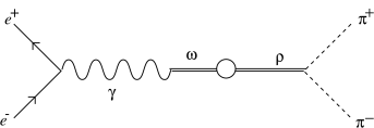
Figure 8: $\rho\!-\!\omega$ mixing contribution to $e^{+}e^{-}\rightarrow\pi^{+}\pi^{-}$.

3.3 Quantum mechanical view of $\rho\!-\!\omega$ mixing

Our initial presentation of $\rho\!-\!\omega$ mixing will follow standard treatments [35, 39] originally due to Coleman and Schnitzer [40]. Although such methods are not usually employed today in the discussion of $\rho\!-\!\omega$ mixing, they contributed significantly to the development of the subject.

The vector meson propagator is given by

$$D_{\mu\nu}(q^{2})=\int d^{4}xe^{-iq\cdot x}\left<0|T\{V_{\mu}(x)V_{\nu}(0)\}|0\right>$$ (78)

which we can rewrite using the spectral representation [17]

$$D_{\mu\nu}(q^{2})=\int_{s_{0}}^{\infty}dr\frac{\sigma(r)}{q^{2}-r}(g_{\mu\nu}-\frac{q_{\mu}q_{\nu}}{r})$$ (79)

where $\sigma(r)$ is the spectral density of the vector states. From Eq. (79) we can define the propagator function, $D(q^{2})$, such that [35]

$$D_{\mu\nu}(q^{2})\equiv D(q^{2})g_{\mu\nu}+\frac{1}{q^{2}}(D(0)-D(s))q_{\mu}q_{\nu}$$ (80)

where we define for convenience here $s\equiv q^{2}$. We now write the propagator function in the following way

$$D(s)=\frac{1}{s-W(s)}\,$$ (81)

where, in what follows, we shall regard $D$ and $W$ as operators. The mass-squared operator, $W$, is a function of $s$ in general and we will later use the form

$$W(s)=m_{0}^{2}+\Pi(s)\;,$$ (82)

where $\Pi(s)$ is the self-energy operator with complex matrix elements and is related to the physical intermediate states (we shall discuss this in section 5.1)). The poles of the matrix elements of $D$ correspond to the physical vector meson states.

If we restrict our attention to the region near the $\omega$ mass, which corresponds to a small energy range (of order $\Gamma_{\omega}$ or $m_{\omega}-m_{\rho}$), we can safely neglect the $s$-dependence of $W$. The decay widths can thus be taken as independent of $s$ in this region.

The physical states can be taken to be linear combinations of the pure isospin states, $|a_{I}\rangle$, $a=\rho,\omega$, where

$$|\rho_{I}\rangle \equiv |1,0\rangle$$

$$|\omega_{I}\rangle \equiv |0,0\rangle$$

in the isospin basis, $|I,I_{3}\rangle$. $W$ and $D$ would be diagonal if there were no isospin-violating effects, but the existence of such effects produces matrix elements which are not diagonal and the off-diagonal elements contain the information about $\rho\!-\!\omega$ mixing. Assuming time reversal invariance these matrix elements are symmetric, though not real (and hence not necessarily hermitian). The physical states are those which diagonalise $W$ and we denote them by $|a\rangle$. Either representation, the physical states $|a\rangle$ or the isospin states $|a_{I}\rangle$ form a complete orthonormal basis; i.e.,

$$I=\sum_{a}|a\rangle\langle a|=\sum_{a_{I}}|a_{I}\rangle\langle a_{I}|$$ (83)

and

$$\delta_{ab}=\langle a|b\rangle=\langle a_{I}|b_{I}\rangle.$$ (84)

Hence the two bases can be related by

$$|a\rangle=\sum_{b_{I}}|b_{I}\rangle\langle b_{I}|a\rangle$$ (85)

and

$$|a_{I}\rangle=\sum_{b}|b\rangle\langle b|a_{I}\rangle$$ (86)

We note here that we define the left eigenvectors $\langle a|$ by these definitions. We will see later that the transformation matrix with elements $\langle b_{I}|a\rangle$ is not unitary and hence $\langle a|\neq(|a\rangle)^{\dagger}$. Naturally, $D(s)$ can be represented in either basis, for example in the physical or mass basis

$$D=\sum_{a,b}|a\rangle\langle a|[s-W(s)]^{-1}|b\rangle\langle b|$$ (87)

with a similar expression using the basis $|a_{I}\rangle$. Since the physical states are those that diagonalise $D$ and $W$ we can write

$$\langle a|W|b\rangle=\delta_{ab}z_{a}$$ (88)

and Eq. (87) becomes

$$D=\sum_{a}\frac{|a\rangle\langle a|}{s-z_{a}}$$ (89)

Since the mixing is observed to be small, we approximate the transformation between the two bases given in Eq. (85) by

$$|\rho\rangle = |\rho_{I}\rangle-\epsilon|\omega_{I}\rangle$$ (90)

$$|\omega\rangle = |\omega_{I}\rangle+\epsilon|\rho_{I}\rangle$$ (91)

where $\epsilon$ is a small, complex mixing parameter. Here and in the following we always work to first order in $\epsilon$. In matrix form, we write

$${\cal C}\equiv\left(\begin{array}[]{cc}\langle\rho_{I}|\rho\rangle&\langle\omega_{I}|\rho\rangle\\ \langle\rho_{I}|\omega\rangle&\langle\omega_{I}|\omega\rangle\end{array}\right)=\left(\begin{array}[]{cc}1&-\epsilon\\ \epsilon&1\end{array}\right)$$ (92)

and

$${\cal W}_{I}\equiv\left(\begin{array}[]{cc}\langle\rho_{I}|W|\rho_{I}\rangle&\langle\rho_{I}|W|\omega_{I}\rangle\\ \langle\omega_{I}|W|\rho_{I}\rangle&\langle\omega_{I}|W|\omega_{I}\rangle\end{array}\right)$$ (93)

where the script letters are used to denote matrices. The physical basis $|\rho\rangle$, $|\omega\rangle$ diagonalises $W$ so we have

$${\cal W}={\cal C}{\cal W}_{I}{\cal C}^{-1}=\left(\begin{array}[]{cc}z_{\rho}&0\\ 0&z_{\omega}\end{array}\right)$$ (94)

from which we deduce, neglecting all terms of order $\epsilon^{2}$ and $\epsilon\langle\rho_{I}|W|\omega_{I}\rangle$ and observing that ${\cal W}_{I}$ must be symmetric so that $\langle\omega_{I}|W|\rho_{I}\rangle=\langle\rho_{I}|W|\omega_{I}\rangle$,

$$\epsilon=\frac{\langle\rho_{I}|W|\omega_{I}\rangle}{z_{\omega}-z_{\rho}}.$$ (95)

Since $z_{a}$ corresponds to the square of the complex mass, it is convenient to write [41]

$$z_{a} = (m_{a}-i\Gamma_{a}/2)^{2}$$ (96)

$$\simeq m_{a}^{2}-im_{a}\Gamma_{a}\,,$$

where $\Gamma_{a}$ is the decay width of particle $a$ which was seen in the form-factor given in Eq. (77). Hence we have

$$\epsilon=\frac{\langle\rho_{I}|W|\omega_{I}\rangle}{m^{2}_{\omega}-m^{2}_{\rho}-i(m_{\omega}\Gamma_{\omega}-m_{\rho}\Gamma_{\rho})}\,.$$ (97)

Now we recall that $W$ is in general momentum dependent, and that we neglected the momentum dependence as a simplification (as we were concerned with only a small region around the $\omega$ mass). Hence, Eq. (97) and therefore $\rho\!-\!\omega$ mixing will, in general, be momentum dependent. Interestingly, $\epsilon$ is seen to have the form (neglecting the $\omega$ width) of a $\rho$ propagator evaluated at $s=m_{\omega}^{2}$, which we can compare with the discussion surrounding Eq. (173).

The amplitude for any process involving intermediate vector states (which mix) will involve matrix elements of the vector meson propagator function, $D$, and can now be written as, using Eq. (89),

$$\langle f|D(s)|i\rangle=\sum_{a}\frac{\langle f|a\rangle\langle a|i\rangle}{s-m_{a}^{2}+im_{a}\Gamma}\,.$$ (98)

For the case of $e^{+}e^{-}\rightarrow\pi^{+}\pi^{-}$, using the more popular second representation of VMD (Eq. (26)) we have

$${\cal M}_{fi} = \langle 2\pi|D(s)|e^{+}e^{-}\rangle$$ (99)

$$= \frac{\langle 2\pi|\rho\rangle\langle\rho|e^{+}e^{-}\rangle}{s-m_{\rho}^{2}+im_{\rho}\Gamma}+\frac{\langle 2\pi|\omega\rangle\langle\omega|e^{+}e^{-}\rangle}{s-m_{\omega}^{2}+im_{\omega}\Gamma}\,.$$

It is from this that we can determine the Orsay phase, $\phi$ [31, 42], which is the relative phase of the $\omega$ and $\rho$ Breit-Wigner amplitudes for $e^{+}e^{-}\rightarrow 2\pi$.

Comparing with Eq. (73) we can identify the pion form factor to be

$$F_{\pi}(s) = \frac{g_{\rho\pi\pi}g_{\rho\gamma}}{s-m^{2}_{\rho}+im_{\rho}\Gamma_{\rho}}+\frac{g_{\omega\pi\pi}g_{\omega\gamma}}{s-m^{2}_{\omega}+im_{\omega}\Gamma_{\omega}}$$ (100)

$$\equiv g_{\rho\pi\pi}g_{\rho\gamma}\left[\frac{1}{s-m^{2}_{\rho}+im_{\rho}\Gamma_{\rho}}\right.\left.+\xi e^{i\phi}\frac{1}{s-m^{2}_{\omega}+im_{\omega}\Gamma_{\omega}}\right],$$

where

$$g_{\rho\gamma}=\frac{m_{\rho}^{2}}{g_{\rho}}.$$

Hence the quantity $\xi e^{i\phi}\equiv(g_{\omega\gamma}/g_{\rho\gamma})(g_{\omega\pi\pi}/g_{\rho\pi\pi})$ governs the shape of the interference and hence of the cross-section around the $\omega$ mass.

In the remainder of the paper, we make use of the following notational conveniences, all valid only when terms of order $\epsilon^{2}$ and $\epsilon\langle\rho_{I}|W|\omega_{I}\rangle$ can be neglected:

$$W_{\rho\rho} \equiv \langle\rho_{I}|W|\rho_{I}\rangle=\langle\rho|W|\rho\rangle=z_{\rho}$$

$$W_{\omega\omega} \equiv \langle\omega_{I}|W|\omega_{I}\rangle=\langle\omega|W|\omega\rangle=z_{\omega}$$

$$W_{\rho\omega} \equiv \langle\rho_{I}|W|\omega_{I}\rangle.$$ (101)

3.4 The contribution of direct omega decay

As had been suggested [34] the existence of a direct decay of the pure isospin state, $\omega_{I}\rightarrow 2\pi$ may have little effect on the decay of the real $\omega$. An argument was given for this [35, 36], and most modern calculations do not include the contribution of the direct decay of the $\omega$. It is useful to outline these arguments and examine whether they still hold for recent examinations of $\rho\!-\!\omega$ mixing.

The coupling of the physical $\omega$ to the two pion state can be expressed as (from Eq. (91))

$${\cal M}_{\omega\pi\pi}={\cal M}_{\omega_{I}\pi\pi}+\epsilon{\cal M}_{\rho_{I}\pi\pi},$$ (102)

where $\epsilon$ is given by Eq. (97). Neglecting the small mass difference of the two mesons and the decay width of the $\omega$ allows us to approximate $\epsilon$, given in Eq. (97), by

$$\epsilon=-i\left(\frac{{\cal R}e\>W_{\rho\omega}+i{\cal I}m\>W_{\rho\omega}}{m_{\rho}\Gamma_{\rho}}\right).$$ (103)

Now assuming the $\omega_{I}$ is able to couple to two pions (afterall, some mechanism is required for CSV), i.e., ${\cal M}_{\omega_{I}\pi\pi}\neq 0$, we would have the mixing interaction, shown in Fig. 9, contributing to $W_{\rho\omega}$, and hence also to $\epsilon$.

Figure 9: Physical intermediate states contributing to $\rho\!-\!\omega$ mixing.

We can determine the contribution to $W_{\rho\omega}$ from $\rho\rightarrow\pi\pi\rightarrow\omega$. To do this, however, it is first useful to consider the analogous case for the simpler $\rho\pi$ system. The self energy of the $\rho$, $W_{\rho\rho}$, is generated by a virtual pion loop as in Fig. 10,

Figure 10: Contribution of a pion loop to the $\rho$ self-energy.

which modifies the $\rho$ propagator in the following way

$$\frac{1}{q^{2}-m_{0}^{2}} \rightarrow \frac{1}{q^{2}-W_{\rho\rho}(q^{2})}$$ (104)

$$\simeq \frac{1}{q^{2}-m_{\rho}^{2}+im_{\rho}\Gamma_{\rho}},$$ (105)

where $m_{0}$ is the bare mass, $m_{\rho}$ the renormalised mass and $\Gamma_{\rho}$ the width of the $\rho$-meson. We now have the definition of the imaginary part of Fig. 10,

$${\cal I}m\;W_{\rho\rho}\equiv-m_{\rho}\Gamma_{\rho}(q^{2}),$$ (106)

where $\Gamma_{\rho}(m_{\rho}^{2})$ is the decay width of the $\rho$. Similarly we can determine the imaginary part of the one-loop diagram shown in Fig. 9, which contributes to ${\cal I}m\;W_{\rho\omega}$. If following the analysis of Renard [35] we assume that the pure isospin decay amplitudes are related by

$${\cal M}_{\rho\omega}=\frac{g_{\omega_{I}\pi\pi}}{g_{\rho_{I}\pi\pi}}{\cal M}_{\rho\rho},$$ (107)

we have

$$W_{\rho\omega}=\frac{g_{\omega_{I}\pi\pi}}{g_{\rho_{I}\pi\pi}}W_{\rho\rho},$$ (108)

and hence

$${\cal I}m\;W_{\rho\omega} = \frac{g_{\omega_{I}\pi\pi}}{g_{\rho_{I}\pi\pi}}{\cal I}m\;W_{\rho\rho}$$ (109)

$$= -\frac{g_{\omega_{I}\pi\pi}}{g_{\rho_{I}\pi\pi}}m_{\rho}\Gamma_{\rho}.$$

Substituting Eq. (109) into Eq. (103) and then substituting that into Eq. (102) we have

$$g_{\omega\pi\pi}=g_{\omega_{I}\pi\pi}-i\frac{{\cal R}e\>W_{\rho\omega}}{m_{\rho}\Gamma_{\rho}}g_{\rho_{I}\pi\pi}+\frac{{\cal I}m\>W_{\rho\omega}}{m_{\rho}\Gamma_{\rho}}g_{\rho_{I}\pi\pi}$$ (110)

Thus

$$g_{\omega\pi\pi}=g_{\omega_{I}\pi\pi}-i\frac{{\cal R}e\>W_{\rho\omega}}{m_{\rho}\Gamma_{\rho}}g_{\rho_{I}\pi\pi}-g_{\omega_{I}\pi\pi}.$$ (111)

As can be seen the contribution from the decay of the $\omega_{I}$ is cancelled.

So, in summary, we allowed CSV through $\omega_{I}\rightarrow\pi\pi$ (in the same form as $\rho_{I}\rightarrow\pi\pi$), which contributed to the mixing parameter, $\epsilon$, through the process depicted in Fig. 9. We then found that the imaginary part of the single pion loop actually cancelled the decay of the $\omega_{I}$ in the process $\omega\rightarrow\pi\pi$. Hence the decay of the the $\omega_{I}$ can be ignored.

However, the approximation of neglecting the $\omega$ width and the $\rho\!-\!\omega$ mass difference in Eq. (103) has recently been re-examined in detail [43]. Without making this approximation it has been found that the $g_{\omega_{I}\pi\pi}$ contribution survives and can contribute significantly.

3.5 Summary

In this section we have concerned ourselves with the initial discovery of the G-parity violating interactions of the $\omega$-meson which could not be explained by electromagnetism alone. We also reviewed the early theoretical attempts to explain these processes. We described the development of the notion of $\rho\!-\!\omega$ mixing, a process which is still not entirely understood at a fundamental level.

It is our purpose in the remainder of this report to develop a simple framework for handling $\rho\!-\!\omega$ mixing and show how to use it in practical calculations.

4 Charge symmetry violation in nuclear physics

Before proceeding to discuss $\rho\!-\!\omega$ mixing in greater detail it is important to briefly review its importance in nuclear physics.

There are a number of fine reviews of charge symmetry and the insight which the small violations of it can give us concerning strongly interacting systems [44, 45, 46]. It would be inappropriate to go over that material at length. Our objective here is simply to recall a few key examples where $\rho\!-\!\omega$ mixing is believed to play an important role. In this way we provide a framework within which our consideration of meson mixing and VMD may be viewed.

The charge symmetry breaking interaction of most interest in nuclear physics has typically been the so-called class-III force [44] which has the form,

$$V^{\rm III}\equiv(\tau_{1z}+\tau_{2z})v_{3}(\mathchoice{\oalign{$\displaystyle r$\crcr\vbox to0.86108pt{\hbox{$\displaystyle\tilde{}$}\vss}}}{\oalign{$\textstyle r$\crcr\vbox to0.86108pt{\hbox{$\textstyle\tilde{}$}\vss}}}{\oalign{$\scriptstyle r$\crcr\vbox to0.86108pt{\hbox{$\scriptstyle\tilde{}$}\vss}}}{\oalign{$\scriptscriptstyle r$\crcr\vbox to0.86108pt{\hbox{$\scriptscriptstyle\tilde{}$}\vss}}},\mathchoice{\oalign{$\displaystyle\sigma_{1}$\crcr\vbox to0.86108pt{\hbox{$\displaystyle\tilde{}$}\vss}}}{\oalign{$\textstyle\sigma_{1}$\crcr\vbox to0.86108pt{\hbox{$\textstyle\tilde{}$}\vss}}}{\oalign{$\scriptstyle\sigma_{1}$\crcr\vbox to0.86108pt{\hbox{$\scriptstyle\tilde{}$}\vss}}}{\oalign{$\scriptscriptstyle\sigma_{1}$\crcr\vbox to0.86108pt{\hbox{$\scriptscriptstyle\tilde{}$}\vss}}},\mathchoice{\oalign{$\displaystyle\sigma_{2}$\crcr\vbox to0.86108pt{\hbox{$\displaystyle\tilde{}$}\vss}}}{\oalign{$\textstyle\sigma_{2}$\crcr\vbox to0.86108pt{\hbox{$\textstyle\tilde{}$}\vss}}}{\oalign{$\scriptstyle\sigma_{2}$\crcr\vbox to0.86108pt{\hbox{$\scriptstyle\tilde{}$}\vss}}}{\oalign{$\scriptscriptstyle\sigma_{2}$\crcr\vbox to0.86108pt{\hbox{$\scriptscriptstyle\tilde{}$}\vss}}}).$$ (112)

This is responsible for the difference between the $nn$, (Coulomb corrected) $pp$ and $np$ scattering lengths. It also contributes to a difference between the masses of mirror nuclei, the famous Okamoto-Nolen-Schiffer (ONS) anomaly [47]. Given our ability to solve the three-body problem, the ${}^{3}{\rm He}-^{3}{\rm H}$ mass difference is the most precisely studied example. After correcting for the EM interaction and the free $n-p$ mass difference there remains some 70 keV to be explained in terms of a charge symmetry violating force [48]. The class-III force associated with $\rho\!-\!\omega$ mixing predicts 90$\pm$14 keV [48] which is in good agreement.

For heavier nuclei the EM corrections are much more difficult to calculate accurately. Nevertheless, after the best estimates have been made a CSV mass difference remains which grows with nuclear mass number, $A$. As illustrated in Table 1 of the results of Blunden and Iqbal [49] (taken from Ref. [50]) a microscopic $NN$ potential, including CSV effects, can account for most of this discrepancy — at least for low $j$. Once again, $\rho\!-\!\omega$ mixing appear to be responsible for the majority (roughly 90%) of the calculated effect.

Nuclear Level		Required CSV (keV)		Calculated CSV (keV)
		DME	SkII	total	$\rho^{0}-\omega$
15	p${}^{-1}_{3/2}$	250	190	210	182
	p${}^{-1}_{1/2}$	380	290	283	227
17	d5/2	300	190	144	131
	1s1/2	320	210	254	218
	d3/2	370	270	246	192
39	1s${}^{-1}_{1/2}$	370	270	337	290
	d${}^{-1}_{3/2}$	540	430	352	281
41	f7/2	440	350	193	175
	1p3/2	380	340	295	258
	1p1/2	410	330	336	282

Table 1: Summary of CSV in the single particle levels for several light nuclei in comparison with the theoretical expectations [49] — from [50].

There has also been considerable experimental activity in the past few years [51, 52] concerning the class-IV force:

$$V^{\rm IV}=(\tau_{1z}-\tau_{2z})(\mathchoice{\oalign{$\displaystyle\sigma$\crcr\vbox to0.86108pt{\hbox{$\displaystyle\tilde{}$}\vss}}}{\oalign{$\textstyle\sigma$\crcr\vbox to0.86108pt{\hbox{$\textstyle\tilde{}$}\vss}}}{\oalign{$\scriptstyle\sigma$\crcr\vbox to0.86108pt{\hbox{$\scriptstyle\tilde{}$}\vss}}}{\oalign{$\scriptscriptstyle\sigma$\crcr\vbox to0.86108pt{\hbox{$\scriptscriptstyle\tilde{}$}\vss}}}_{1}-\mathchoice{\oalign{$\displaystyle\sigma$\crcr\vbox to0.86108pt{\hbox{$\displaystyle\tilde{}$}\vss}}}{\oalign{$\textstyle\sigma$\crcr\vbox to0.86108pt{\hbox{$\textstyle\tilde{}$}\vss}}}{\oalign{$\scriptstyle\sigma$\crcr\vbox to0.86108pt{\hbox{$\scriptstyle\tilde{}$}\vss}}}{\oalign{$\scriptscriptstyle\sigma$\crcr\vbox to0.86108pt{\hbox{$\scriptscriptstyle\tilde{}$}\vss}}}_{2})\cdot\mathchoice{\oalign{$\displaystyle L$\crcr\vbox to0.86108pt{\hbox{$\displaystyle\tilde{}$}\vss}}}{\oalign{$\textstyle L$\crcr\vbox to0.86108pt{\hbox{$\textstyle\tilde{}$}\vss}}}{\oalign{$\scriptstyle L$\crcr\vbox to0.86108pt{\hbox{$\scriptstyle\tilde{}$}\vss}}}{\oalign{$\scriptscriptstyle L$\crcr\vbox to0.86108pt{\hbox{$\scriptscriptstyle\tilde{}$}\vss}}}v(r)+(\vec{\tau}_{1}\times\vec{\tau}_{2})_{z}(\mathchoice{\oalign{$\displaystyle\sigma$\crcr\vbox to0.86108pt{\hbox{$\displaystyle\tilde{}$}\vss}}}{\oalign{$\textstyle\sigma$\crcr\vbox to0.86108pt{\hbox{$\textstyle\tilde{}$}\vss}}}{\oalign{$\scriptstyle\sigma$\crcr\vbox to0.86108pt{\hbox{$\scriptstyle\tilde{}$}\vss}}}{\oalign{$\scriptscriptstyle\sigma$\crcr\vbox to0.86108pt{\hbox{$\scriptscriptstyle\tilde{}$}\vss}}}_{1}\times\mathchoice{\oalign{$\displaystyle\sigma$\crcr\vbox to0.86108pt{\hbox{$\displaystyle\tilde{}$}\vss}}}{\oalign{$\textstyle\sigma$\crcr\vbox to0.86108pt{\hbox{$\textstyle\tilde{}$}\vss}}}{\oalign{$\scriptstyle\sigma$\crcr\vbox to0.86108pt{\hbox{$\scriptstyle\tilde{}$}\vss}}}{\oalign{$\scriptscriptstyle\sigma$\crcr\vbox to0.86108pt{\hbox{$\scriptscriptstyle\tilde{}$}\vss}}}_{2})\cdot\mathchoice{\oalign{$\displaystyle L$\crcr\vbox to0.86108pt{\hbox{$\displaystyle\tilde{}$}\vss}}}{\oalign{$\textstyle L$\crcr\vbox to0.86108pt{\hbox{$\textstyle\tilde{}$}\vss}}}{\oalign{$\scriptstyle L$\crcr\vbox to0.86108pt{\hbox{$\scriptstyle\tilde{}$}\vss}}}{\oalign{$\scriptscriptstyle L$\crcr\vbox to0.86108pt{\hbox{$\scriptscriptstyle\tilde{}$}\vss}}}w(r),$$ (113)

where vectors in isospin-space have been denoted by overhead arrows, and those in position space by underlining. Such a force only affects the $np$ system where it mixes the spin singlet and triplet channels [53]. It turns out that at TRIUMF energies [51] the measurement is insensitive to $\rho\!-\!\omega$ mixing and agrees well with the theoretical expectations [53]. On the other hand, at the IUCF energy [52] the data agrees well with the theoretical prediction [53, 54], about half of which can be explained in terms of $\rho\!-\!\omega$ mixing. Unfortunately, the experimental error is such that this is only a $1.5$ standard deviation effect. It would be very informative to reduce the errors by a factor of 2-3 in the IUCF energy region.

Clearly there are a number of examples where CSV in nuclear physics seems to require the contribution to the $NN$ force arising from $\rho\!-\!\omega$ mixing. In order to calculate such a force one must take the Fourier transform of the Feynman diagram shown in Fig. 11.

Figure 11: CSV in the nuclear potential resulting from $\rho\!-\!\omega$ mixing.

Schematically this involves [55]:

$$V_{\rm CSV}(r)\propto\frac{1}{r}\int_{-\infty}^{\infty}dq\;q\frac{\sin(qr)\Pi_{\rho\omega}(-q^{2})}{(q^{2}+m_{\rho}^{2})(q^{2}+m_{\omega}^{2})}$$ (114)

where $\Pi_{\rho\omega}(-q^{2})$ is the $\rho\!-\!\omega$ mixing amplitude in the space-like region. Traditionally this has been evaluated using contour integration and keeping only the poles associated with the vector meson propagator. That is, $V_{\rm CSV}$ is proportional to $\Pi_{\rho\omega}(m_{\rho}^{2})$, the mixing amplitude at the $\rho$ (or the $\omega$) pole. If $\Pi_{\rho\omega}$ were to vary rapidly between the time-like and space-like regions, as first suggested by Goldman et al. [56], this would be a very bad approximation. Indeed, if the behaviour found by Goldman et al. (discussed in the next section) were correct, $\rho\!-\!\omega$ mixing would contribute little or nothing in the example we have just considered [57]. One would then be faced with the task of finding alternative, possibly quark-level [58, 59, 65, 66], explanations. In any case, one would be forced to re-examine the understanding of nuclear matter at a fairly fundamental level.

5 The behaviour of $\rho\!-\!\omega$ mixing

The various proposed mechanisms for $\rho\!-\!\omega$ mixing (as, for example, the pion loops of Fig. 9) would have inescapably led to the conclusion that it was a momentum dependent process. However no direct calculations were ever made of these loop diagrams.

In the early studies of $\rho\!-\!\omega$ mixing the mixing parameter $\epsilon$ (c.f. Eqs. (90) and (91)) was never precluded from being momentum dependent. Unfortunately, experimental limitations meant there was little hope that much could be known about $\epsilon$ away from the $\rho$ mass. Faced with this constraint it seemed sensible to devote ones energies to finding out as much as possible about the mixing process at $q^{2}=m_{\omega}^{2}$. The information came exclusively from the decay $\omega\rightarrow\pi^{+}\pi^{-}$, i.e. two pion production at the $\omega$ mass point, which (as we discussed) was believed to be entirely due to mixing. (Note, though, that recently there has been some discussion of the experimentally more difficult $\rho\rightarrow 3\pi$ decay [67].) Renard [35] gives a discussion of the behaviour of the mixing, in terms of $W$ in Eq. (82). He explains that there were two approximations made for the momentum dependence. The first was to ignore any momentum dependence, the second was to assume it was linear (in which case it would vanish for $s=0$, as predicted in section 5.1).

As time went by any thought of $\epsilon$ being anything other than a fixed parameter that could be cleanly extracted from processes involving the two pion decay of the $\omega$ simply fell by the wayside (much like the first representation of VMD).

While this has little effect for something such as the EM form factor of the pion, its eventual application [68] to the spacelike world of nuclear physics where it has been incorporated into the meson exchange model was cause for if not concern, at least caution. However, the success of this assumption (outlined in Sec.  4) has been seen as a compelling justification.

The question of momentum dependence in $\rho\!-\!\omega$ mixing was first asked by Goldman, Henderson and Thomas (GHT) [56] and has generated a significant amount of work. The initial GHT model was relatively simple. The vector mesons were assumed to be quark-antiquark composites, and the mixing was generated entirely by the small mass difference between the up and down quark masses. The mesons coupled to the quark loop via a form-factor $F(k^{2})$ where $k_{\mu}$ is the free momentum of the quark loop, which models the finite size of the meson substructure. Free Dirac propagators were used for the quarks, thus ignoring the question of confinement. More recent work [69, 70] has modelled confinement by using quark propagators which are entire (i.e. they do not have a pole in the complex $q^{2}$ plane and thus the quarks are never on mass-shell). The vector mesons couple to conserved currents which, as will be shown later, leads to a node in the mixing when the momentum squared ($q^{2}$) of the meson vanishes [71]. A gauge invariant model, will produce a node at $q^{2}=0$ (see next section). However the form-factors used in the GHT model spoil gauge invariance, and thus their node is shifted slightly away from $q^{2}=0$.

The use of an intermediate nucleon loop [72] as the mechanism driving $\rho\!-\!\omega$ mixing (relying on the mass difference between the neutron and proton) avoids the worries of quark confinement, as well as enabling one to use well-known parameters in the calculation (masses, couplings, etc). This model has a node for the mixing at $q^{2}=0$. Mitchell et al. [70] concluded that in their bi-local theory (where the meson fields are composites of quark operators, e.g. $\omega_{\mu}(x,y)\sim\overline{q}(y)i\gamma_{\mu}q(x)$) the quark loop mechanism alone generates an insignificant charge symmetry breaking potential and suggest a pion loop contribution should be examined [73], which is interesting in the light of our discussion (Sec. 3.4) about the contribution of the direct $\omega$ decay. Subsequent calculations using the Nambu–Jona-Lasinio model [74], chiral perturbation theory [75, 76, 77], QCD sum rules [76, 78, 79, 80] and quark models [81] have explored aspects of $\rho\!-\!\omega$ mixing, including its momentum dependence.

Iqbal and Niskanen [57] have studied the effect of a varying $\rho\!-\!\omega$ mixing for neutron-proton scattering. Using a model for the variation [78] they conclude that it would significantly alter our understanding of how to model the charge-symmetry breaking effects in the strong nuclear interaction.

5.1 General Considerations

We review our proof [71] that the mixing amplitude vanishes at $q^{2}=0$ in any effective Lagrangian model (e.g., ${\cal L}(\vec{\rho},\omega,\vec{\pi},\bar{\psi},\psi,\cdots)$), where there are no explicit mass mixing terms (e.g., $m^{2}_{\rho\omega}\rho^{0}_{\mu}\omega^{\mu}$ or $\sigma\rho^{0}_{\mu}\omega^{\mu}$ with $\sigma$ some scalar field) in the bare Lagrangian and where the vector mesons have a local coupling to conserved currents which satisfy the usual vector current commutation relations. The boson-exchange model of Ref. [72] where, e.g., $J^{\mu}_{\omega}=g_{\omega}\bar{N}\gamma^{\mu}N$, is one particular example. It follows that the mixing tensor (analogous to the full self-energy function for a single vector boson such as the $\rho$ [82])

$$C^{\mu\nu}(q)=i\int d^{4}x\,e^{iq\cdot x}\left<0\right|T(J^{\mu}_{\rho}(x)J^{\nu}_{\omega}(0))\left|0\right>.$$ (115)

is transverse. Here, the operator $J^{\mu}_{\omega}$ is the operator appearing in the equation of motion for the field operator $\omega$ — c.f. Eq. (14). Note that when $J^{\mu}_{\omega}$ is a conserved current then $\partial_{\mu}J^{\mu}_{\omega}=0$, which ensures that the Proca equation leads to the same subsidiary condition as the free field case, $\partial_{\mu}\omega^{\mu}=0$ (see, e.g., Lurie, pp. 186–190 [17], or other field theory texts [21, 83]). The operator $J^{\mu}_{\rho}$ is similarly defined. We see then that $C^{\mu\nu}$ can be written in the form,

$$C^{\mu\nu}(q)=\left(g^{\mu\nu}-{q^{\mu}q^{\nu}\over q^{2}}\right)C(q^{2})\,.$$ (116)

From this it follows that the one-particle-irreducible self-energy or polarisation, $\Pi^{\mu\nu}(q)$ (defined through Eq. (120) below), must also be transverse [82]. The essence of the argument below is that since there are no massless, strongly interacting vector particles $\Pi^{\mu\nu}$ cannot be singular at $q^{2}=0$ and therefore $\Pi(q^{2})$ (see Eq. (121) below) must vanish at $q^{2}=0$, as suggested for the pure $\rho$ case [19]. As we have already noted this is something that was approximately true in all models, but guaranteed only in Ref. [72].

Let us briefly recall the proof of the transversality of $C^{\mu\nu}(q)$. As shown, for example, by Itzykson and Zuber (pp. 217–224) [20], provided we use covariant time-ordering the divergence of $C^{\mu\nu}$ leads to a naive commutator of the appropriate currents

$$q_{\mu}C^{\mu\nu}(q) = -\int d^{4}x\,e^{iq\cdot x}\partial_{\mu}\;\{\theta(x^{0})\left<0\right|J^{\mu}_{\rho}(x)J^{\nu}_{\omega}(0)\left|0\right>$$ (117)

$$+\;\theta(-x^{0})\left<0\right|J^{\nu}_{\omega}(0)J^{\mu}_{\rho}(x)\left|0\right>\}$$

$$= -\int d^{3}x\,e^{i\vec{q}\cdot\vec{x}}\left<0\right|[J^{0}_{\rho}(0,\vec{x}),J^{\nu}_{\omega}(0)]\left|0\right>_{\rm naive}.$$ (118)

That is, there is a cancellation between the seagull and Schwinger terms. Thus, for any model in which the isovector- and isoscalar- vector currents satisfy the same commutation relations as QCD we find

$$q_{\mu}C^{\mu\nu}(q)=0.$$ (119)

Thus, by Lorentz invariance, the tensor must be of the form given in Eq. (116).

For simplicity we consider first the case of a single vector meson (e.g. a $\rho$ or $\omega$) without channel coupling. For such a system one can readily see that since $C^{\mu\nu}$ is transverse the one-particle irreducible self-energy, $\Pi^{\mu\nu}$, defined through [82]

$$\Pi^{\mu\alpha}D_{\alpha\nu}=C^{\mu\alpha}D^{0}_{\alpha\nu}$$ (120)

(where $D$ and $D^{0}$ are defined below) is also transverse. Hence

$$\Pi^{\mu\nu}(q)=\left(g^{\mu\nu}-{q^{\mu}q^{\nu}\over q^{2}}\right)\Pi(q^{2})\,.$$ (121)

We are now in a position to establish the behaviour of the scalar function, $\Pi(q^{2})$. In a general theory of massive vector bosons coupled to a conserved current, the bare propagator has the form (compared to Eq. (74) for the photon)

$$D^{0}_{\mu\nu}=\left(-g_{\mu\nu}+{q_{\mu}q_{\nu}\over m^{2}}\right){1\over{q^{2}-m^{2}}}$$ (122)

whence

$$(D^{0})^{-1}_{\mu\nu}=(m^{2}-q^{2})g_{\mu\nu}+q_{\mu}q_{\nu}.$$ (123)

The polarisation is incorporated in the standard way to give the dressed propagator

$$iD_{\mu\nu}=iD_{\mu\nu}^{0}+iD_{\mu\alpha}^{0}i\Pi^{\alpha\beta}iD_{\beta\nu}^{0}+\cdots$$ (124)

We now use the operator identity of Eq. (31) to give

$$D^{-1}_{\mu\nu} = (D^{0})^{-1}_{\mu\nu}+\Pi_{\mu\nu}$$ (125)

$$= (m^{2}-q^{2}+\Pi(q^{2}))g_{\mu\nu}+\left(1-{\Pi(q^{2})\over q^{2}}\right)q_{\mu}q_{\nu}.$$

Thus the full propagator has the form

$$D_{\mu\nu}(q)={-g_{\mu\nu}+\left(1-\Pi(q^{2})/q^{2}\right)(q_{\mu}q_{\nu}/m^{2})\over q^{2}-m^{2}-\Pi(q^{2})}.$$ (126)

Having established this form for the propagator, we wish to compare it with the Renard spectral representation of the propagator given by Eq. (80). By comparing the coefficients of $g_{\mu\nu}$ in Eqs. (126) and (80) we deduce

$$D(q^{2})={-1\over{q^{2}-m^{2}-\Pi(q^{2})}}\,,$$ (127)

while from the coefficients of $q_{\mu}q_{\nu}$ we have

$${\left(1-{\Pi(q^{2})/q^{2}}\right)\over{(q^{2}-m^{2}-\Pi(q^{2}))m^{2}}} = {1\over q^{2}}(D(0)-D(q^{2}))$$ (128)

$$= {1\over q^{2}}{q^{2}+\Pi(0)-\Pi(q^{2})\over(m^{2}+\Pi(0))(q^{2}-m^{2}-\Pi(q^{2}))},$$

from which we obtain

$$\frac{\Pi(0)}{q^{2}}(q^{2}-m^{2}-\Pi(q^{2}))=0\,\,\,\,\,\,\,\,,\,\,\,\,\,\forall q^{2}$$ (129)

and thus

$$\Pi(0)=0.$$ (130)

This is an important constraint on the self-energy function, namely that $\Pi(q^{2})$ should vanish as $q^{2}\rightarrow 0$ at least as fast as $q^{2}$.

While the preceding discussion dealt with the single channel case, for $\rho-\omega$ mixing we are concerned with two coupled channels. Our calculations therefore involve matrices. As we now demonstrate, this does not change our conclusion.

The matrix analogue of Eq. (125) is

$$D^{-1}_{\mu\nu}=\left(\begin{array}[]{cc}m_{\rho}^{2}g_{\mu\nu}+(\Pi_{\rho\rho}(q^{2})-q^{2})T_{\mu\nu}&\Pi_{\rho\omega}(q^{2})T_{\mu\nu}\\ \Pi_{\rho\omega}(q^{2})T_{\mu\nu}&m_{\omega}^{2}g_{\mu\nu}+(\Pi_{\omega\omega}(q^{2})-q^{2})T_{\mu\nu}\end{array}\right),$$ (131)

where we have defined $T_{\mu\nu}\equiv g_{\mu\nu}-(q_{\mu}q_{\nu}/q^{2}$) for brevity. By obtaining the inverse of this we have the two-channel propagator

$$D_{\mu\nu}=\frac{1}{\alpha}\left(\begin{array}[]{cc}s_{\omega}g_{\mu\nu}+a(\rho,\omega)q_{\mu}q_{\nu}&\Pi_{\rho\omega}(q^{2})T_{\mu\nu}\\ \Pi_{\rho\omega}(q^{2})T_{\mu\nu}&s_{\rho}g_{\mu\nu}+a(\omega,\rho)q_{\mu}q_{\nu}\end{array}\right),$$ (132)

where

$$s_{\omega} \equiv q^{2}-\Pi_{\omega\omega}(q^{2})-m_{\omega}^{2}$$ (133)

$$s_{\rho} \equiv q^{2}-\Pi_{\rho\rho}(q^{2})-m_{\rho}^{2}$$ (134)

$$a(\rho,\omega) \equiv \frac{1}{q^{2}m_{\rho}^{2}}\{\Pi_{\rho\omega}^{2}(q^{2})-[q^{2}-\Pi_{\rho\rho}(q^{2})]s_{\omega}\}$$ (135)

$$\alpha \equiv \Pi_{\rho\omega}^{2}(q^{2})-s_{\rho}s_{\omega}.$$ (136)

In the uncoupled case [$\Pi_{\rho\omega}(q^{2})=0$] Eq. (132) clearly reverts to the appropriate form of the one particle propagator, Eq. (126), as desired.

We can now make the comparison between Eq. (132) and the Renard form [35] of the propagator, as given by Eq. (80). The transversality of the off-diagonal terms of the propagator, demands that $\Pi_{\rho\omega}(0)=0$. A similar analysis leads one to conclude the same for $\Pi_{\rho\rho}(q^{2})$ and $\Pi_{\omega\omega}(q^{2})$. Note that the physical $\rho^{0}$ and $\omega$ masses which arise from locating the poles in the diagonalised propagator matrix $D^{\mu\nu}$ no longer correspond to exact isospin eigenstates (as in the discussion of the historical treatment of $\rho\!-\!\omega$ mixing, Sec. 3.3). To lowest order in CSV the physical $\rho$-mass is given by $m^{\rm phys}_{\rho}=[m^{2}_{\rho}+\Pi_{\rho\rho}((m^{\rm phys}_{\rho})^{2})]^{1/2}$, i.e., the pole in $D^{\mu\nu}_{\rho\rho}$. The physical $\omega$-mass is similarly defined.

In conclusion, it is important to review what has and has not been established. There is no unique way to derive an effective field theory including vector mesons from QCD. Our result that $\Pi_{\rho\omega}(0)$ (as well as $\Pi_{\rho\rho}(0)$ and $\Pi_{\omega\omega}(0)$) should vanish applies to those effective theories in which: (i) the vector mesons have local couplings to conserved currents which satisfy the same commutation relations as QCD [i.e., Eq. (118) is zero] and (ii) there is no explicit mass-mixing term in the bare Lagrangian. This includes a broad range of commonly used, phenomenological theories. It does not include the model treatment of Ref. [70] for example, where the mesons are bi-local objects in a truncated effective action. However, it is interesting to note that a node near $q^{2}=0$ was found in this model in any case. The presence of an explicit mass-mixing term in the bare Lagrangian will shift the mixing amplitude by a constant (i.e., by $m_{\rho\omega}^{2}$). We believe that such a term will lead to difficulties in matching the effective model onto the known behaviour of QCD in the high-momentum limit.

Finally the fact that $\Pi(q^{2})$ is momentum-dependent or vanishes everywhere in this class of models implies that the conventional assumption of a non-zero, constant $\rho-\omega$ mixing amplitude remains questionable. This study then lends support to those earlier calculations, which we briefly discussed, where it was concluded that the mixing may play a minor role in the explanation of CSV in nuclear physics. It remains an interesting challenge to find possible alternate mechanisms to describe charge-symmetry violation in the $NN$-interaction [58, 59, 60, 61, 62, 63, 64].

5.2 The mixed propagator approach to $\rho\!-\!\omega$ mixing

Different authors parameterise the $\rho\!-\!\omega$ mixing contribution to the pion form-factor in one of two ways. Using the matrix method we shall show here the connection between these two models, both of which are first order in charge symmetry breaking.

Using a matrix notation, the Feynman amplitude for the process $\gamma\rightarrow\pi\pi$, proceeding via vector mesons, can be written in the form

$$i{\cal M}_{\mu;\gamma\rightarrow\pi\pi}=\left(\begin{array}[]{cc}i{\cal M}^{\nu}_{\rho_{I}\rightarrow\pi\pi}&i{\cal M}^{\nu}_{\omega_{I}\rightarrow\pi\pi}\end{array}\right)iD_{\nu\mu}\left(\begin{array}[]{c}i{\cal M}_{\gamma\rightarrow\rho_{I}}\\ i{\cal M}_{\gamma\rightarrow\omega_{I}}\end{array}\right)$$ (137)

where the matrix $D_{\nu\mu}$ is given by Eq. (132) and the other Feynman amplitudes are derived from either the VMD1 or VMD2 Lagrangian (Eqs. (25) and (26). Since we always couple the vector mesons to conserved currents, the terms proportional to $q_{\mu}q_{\nu}$ in the propagator (Eq. (132)) can always be neglected. If we assume that the pure isospin state $\omega_{I}$ does not couple to two pions (${\cal M}^{\nu}_{\omega_{I}\rightarrow\pi\pi}=0$) then to lowest order in the mixing, Eq. (137) is just

$${\cal M}^{\mu}_{\gamma\rightarrow\pi\pi}=\left(\begin{array}[]{cc}{\cal M}^{\mu}_{\rho_{I}\rightarrow\pi\pi}&0\end{array}\right)\left(\begin{array}[]{cc}1/s_{\rho}&\Pi_{\rho\omega}/s_{\rho}s_{\omega}\\ \Pi_{\rho\omega}/s_{\rho}s_{\omega}&1/s_{\omega}\end{array}\right)\left(\begin{array}[]{c}{\cal M}_{\gamma\rightarrow\rho_{I}}\\ {\cal M}_{\gamma\rightarrow\omega_{I}}\end{array}\right)$$ (138)

Expanding this just gives

$${\cal M}^{\mu}_{\gamma\rightarrow\pi\pi}={\cal M}^{\mu}_{\rho_{I}\rightarrow\pi\pi}\frac{1}{s_{\rho}}{\cal M}_{\gamma\rightarrow\rho_{I}}+{\cal M}^{\mu}_{\rho_{I}\rightarrow\pi\pi}\frac{1}{s_{\rho}}\Pi_{\rho\omega}\frac{1}{s_{\omega}}{\cal M}_{\gamma\rightarrow\omega_{I}}$$ (139)

which we recognise as the sum of the two diagrams shown in Fig. 12.

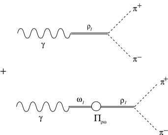
Figure 12: The contribution of $\rho\!-\!\omega$ mixing to the pion form-factor.

The couplings that enter this expression, through ${\cal M}^{\mu}_{\rho_{I}\rightarrow\pi\pi}$, ${\cal M}_{\gamma\rightarrow\rho_{I}}$ and ${\cal M}_{\gamma\rightarrow\omega_{I}}$, always involve the unphysical pure isospin states $\rho_{I}$ and $\omega_{I}$. However, we can re-express Eq. (139) in terms of the physical states by first diagonalising the vector meson propagator. Following the same procedure as in Sec. 3.3, we introduce a diagonalising matrix

$$C=\left(\begin{array}[]{cc}1&\epsilon\\ -\epsilon&1\end{array}\right)$$ (140)

where, to lowest order in the mixing,

$$\epsilon=\frac{\Pi_{\rho\omega}}{s_{\rho}-s_{\omega}}.$$ (141)

We now insert identities into Eq. (138) and obtain

$${\cal M}^{\mu}_{\gamma\rightarrow\pi\pi} = \left(\begin{array}[]{cc}{\cal M}^{\mu}_{\rho_{I}\rightarrow\pi\pi}&0\end{array}\right)CC^{-1}\left(\begin{array}[]{cc}1/s_{\rho}&\Pi_{\rho\omega}/s_{\rho}s_{\omega}\\ \Pi_{\rho\omega}/s_{\rho}s_{\omega}&1/s_{\omega}\end{array}\right)CC^{-1}\left(\begin{array}[]{c}{\cal M}_{\gamma\rightarrow\rho_{I}}\\ {\cal M}_{\gamma\rightarrow\omega_{I}}\end{array}\right)$$ (147)

$$= \left(\begin{array}[]{cc}{\cal M}^{\mu}_{\rho\rightarrow\pi\pi}&{\cal M}^{\mu}_{\omega\rightarrow\pi\pi}\end{array}\right)\left(\begin{array}[]{cc}1/s_{\rho}&0\\ 0&1/s_{\omega}\end{array}\right)\left(\begin{array}[]{c}{\cal M}_{\gamma\rightarrow\rho}\\ {\cal M}_{\gamma\rightarrow\omega}\end{array}\right)$$ (153)

where we have identified the physical amplitudes as

$${\cal M}^{\mu}_{\rho\rightarrow\pi\pi} = {\cal M}^{\mu}_{\rho_{I}\rightarrow\pi\pi},$$ (154)

$${\cal M}^{\mu}_{\omega\rightarrow\pi\pi} = \epsilon{\cal M}^{\mu}_{\rho_{I}\rightarrow\pi\pi},$$ (155)

$${\cal M}_{\gamma\rightarrow\rho} = {\cal M}_{\gamma\rightarrow\rho_{I}}-\epsilon{\cal M}_{\gamma\rightarrow\omega_{I}},$$ (156)

$${\cal M}_{\gamma\rightarrow\omega} = {\cal M}_{\gamma\rightarrow\omega_{I}}+\epsilon{\cal M}_{\gamma\rightarrow\rho_{I}}.$$ (157)

Expanding Eq. (153), we find

$${\cal M}^{\mu}_{\gamma\rightarrow\pi\pi} = {\cal M}^{\mu}_{\rho\rightarrow\pi\pi}\frac{1}{s_{\rho}}{\cal M}_{\gamma\rightarrow\rho}+{\cal M}^{\mu}_{\omega\rightarrow\pi\pi}\frac{1}{s_{\omega}}{\cal M}_{\gamma\rightarrow\omega}$$ (158)

$$= {\cal M}^{\mu}_{\rho\rightarrow\pi\pi}\frac{1}{s_{\rho}}{\cal M}_{\gamma\rightarrow\rho}+{\cal M}^{\mu}_{\rho\rightarrow\pi\pi}\frac{\Pi_{\rho\omega}}{s_{\rho}-s_{\omega}}\frac{1}{s_{\omega}}{\cal M}_{\gamma\rightarrow\omega},$$

which is the usually seen in older works. At first glance there seems to be a slight discrepancy between Eqs. (139) and (158). The source of this is the definition used for the coupling of the vector meson to the photon. The first, Eq. (139), uses couplings to pure isospin states, the second, Eq. (158) uses “physical” couplings (i.e., couplings to the mass eigenstates) which introduce a leptonic contribution to the Orsay phase, as discussed by Coon et al. [55]. This phase is, however, rather small. If we assume ${\cal M}_{\gamma\rightarrow\rho_{I}}=3{\cal M}_{\gamma\rightarrow\omega_{I}}$ and define the leptonic phase $\theta$ by

$$\frac{{\cal M}_{\gamma\rightarrow\omega}}{{\cal M}_{\gamma\rightarrow\rho}}=\frac{1}{3}e^{i\theta}$$ (159)

then, to order $\epsilon$,

$$\tan\theta=\frac{10\Pi_{\rho\omega}}{3m_{\rho}\Gamma_{\rho}}.$$ (160)

This gives $\theta=5.7^{o}$ for $\Pi_{\rho\omega}=-4520$, as obtained by Coon et al. [55]. This small leptonic contribution to the Orsay phase is the principal manifestation of diagonalising the $\rho\!-\!\omega$ propagator.

6 Phenomenological analysis of $F_{\pi}$

In this section we discuss various methods for both fitting the pion form factor and obtaining the numerical value of $\Pi_{\rho\omega}$. We extract $\Pi_{\rho\omega}$ with a fit to the pion form-factor (using VMD1), but, as will be seen, this is not the method used to obtain the most widely quoted value.

Recent analysis of the $e^{+}e^{-}\rightarrow\pi^{+}\pi^{-}$data give us an insight into how successful the second formulation has been in describing the process. We find that in both cases studied a non-resonant contribution has been included to optimise the fit, in direct contrast with the spirit of the second formulation. Following this we present an example of the use of the first formulation to plot the curve for the cross-section of $e^{+}e^{-}\rightarrow\pi^{+}\pi^{-}$.

6.1 Recent fits

Benayoun et al. [84] examine $e^{+}e^{-}\rightarrow\pi^{+}\pi^{-}$in an effort to better understand the process $\eta^{\prime}\rightarrow\pi^{+}\pi^{-}\gamma$, which requires a thorough understanding of $\rho$ physics, i.e. how to effectively parameterise it, and whether to include any non-resonant contributions to the process. They are concerned primarily with fitting the data, relying on as much experimental input as possible, rather than trying to test the behaviour of a particular model for the process (which is our intention).

Their expression for the amplitude takes the form described in Eq. (73), with

$$F_{\pi}(s)(p_{3}-p_{4})_{\mu} = \left[A(q^{2})\Sigma_{j}\epsilon^{j}_{\mu}(\gamma)\epsilon^{j*}_{\nu}(\gamma)+\!g_{\rho\gamma}\frac{1}{m_{\rho}^{2}-q^{2}-im_{\rho}\Gamma_{\rho}(q^{2})}G_{\rho}\Sigma_{j}\epsilon^{j}_{\mu}(\rho)\epsilon^{j*}_{\nu}(\rho)\right.$$ (161)

$$+ \left.g_{\omega\gamma}\frac{e^{i\phi}}{m_{\omega}^{2}-q^{2}-im_{\omega}\Gamma_{\omega}}G_{\omega}\Sigma_{j}\epsilon^{j}_{\mu}(\omega)\epsilon^{j*}_{\nu}(\omega)\right](p_{3}-p_{4})^{\nu},$$

where $j$ is the index associated with the helicity of the polarisation vectors $\epsilon_{\mu}$. The first term, $A(q^{2})$, introduces their proposed non-resonant contribution to $F_{\pi}(q^{2})$. Note the use of the momentum dependent width for the $\rho$ but not the $\omega$ (as its major decay channel, $3\pi$, is not included in the $2\pi$ data analysed, and one can, as an approximation, ignore the momentum dependence of the width). The width was taken to be [84]

$$\Gamma_{\rho}(q^{2})=\Gamma_{\rho}\left(\frac{k(q^{2})}{k(m_{\rho}^{2})}\right)^{3}\left(\frac{m_{\rho}}{\sqrt{q^{2}}}\right)^{\lambda}$$ (162)

where $\lambda$ is a parameter for fitting,

$$k(q^{2})=\frac{1}{2}\sqrt{q^{2}-4m_{\pi}^{2}},$$ (163)

and

$$G_{V}=\frac{1}{k^{3/2}(q^{2})}\sqrt{6\pi m_{V}\sqrt{q^{2}}\Gamma_{V\pi^{+}\pi^{-}}}.$$ (164)

Note that, because of $k(q^{2})$ in Eq. (163), the width, $\Gamma_{\rho}(q^{2})$ given in Eq. (162), will become imaginary below threshold, i.e., $q^{2}=4m_{\pi}^{2}$. Considering Eq. (161), the width contribution to the denominator of the propagator (Eq. (162)) will actually become real and add to the mass term below threshold. The use of a term such as $\theta(q^{2}-4m_{\pi}^{2})$ in Eq. (162) would spoil the analytic continuation of the propagator below threshold. The width of the $\rho$ is almost entirely due to the two pion decay, and thus the full width can be used in Eq. (164) to determine $G_{\rho}$. However this is not the case for the $\omega$, so one has to make the appropriate modification

$$\Gamma_{\omega}(q^{2})={\rm BR}(\omega\rightarrow\pi^{+}\pi^{-})\Gamma_{\omega}\left(\frac{k(q^{2})}{k(m_{\omega}^{2})}\right)^{3}\left(\frac{m_{\omega}}{\sqrt{q^{2}}}\right)^{\lambda},$$ (165)

where ${\rm BR}(\omega\rightarrow\pi^{+}\pi^{-})$ is the branching ratio for the decay. Note that Eq. (161) uses the full width of the $\omega$, rather than the branching fraction as in Eq. (164). This is because the width appearing in the propagator measures the flux loss due to the decay of the particle irrespective of its decay channel. Conversely, $G_{\omega}$ describes the coupling of the $\omega$ to two pions only, so the partial width must be used.

The form-factor is thus

$$F_{\pi}(q^{2})=A(q^{2})-\frac{g_{\rho\gamma}}{s_{\rho}}G_{\rho}-\frac{g_{\omega\gamma}}{s_{\omega}}e^{i\phi}G_{\omega}.$$ (166)

The resemblance of Eq. (166) to the older form given in Eq. (100) is immediately apparent (i.e. the sum of the $\rho$ contribution and an Orsay-phased $\omega$ contribution). This can now be used in Eq. (76) to compute the cross-section.

Benayoun et al. [84] now proceed along two paths, using the accepted figures for the $\omega$ as well as both leptonic decay widths (which are assumed to be fairly well understood):

a) fitting the $\rho$ parameters and the Orsay phase, $\phi$, assuming $A=0$;

b) fitting $A$ and leaving the $\rho$ mass fixed at the world average, 768.7$\pm$0.7 MeV, as it is believed to be less sensitive than the width to parametrisation.

For the first case they arrive at values for the mass and width slightly higher than usually found using the Gounaris-Sakurai model [30] by, for example, Barkhov et al. [85].

For the second case, $A$ is assumed to take the form

$$A(q^{2})=-(c_{0}+c_{2}q^{2}+c_{4}q^{4}+\cdots).$$ (167)

The expansion is stopped as soon as the effect of the next term is negligible. At this point Benayoun et al. pause to relect on the condition $F_{\pi}(0)=1$. $A(0)$, as determined by their fit, would contribute 0.607 to $F_{\pi}(0)$. They dismiss the relevance of this as they are using “an expansion valid in the range $(\sqrt{s}=)\;[2m_{\pi},m_{\eta^{\prime}}]$.” They go on to point out that a good fit (which, in addition, reproduces values for the parameters closer to the usual ones) can be obtained using

$$A(q^{2})=\frac{-1}{1+q^{2}/m_{\rho}^{2}}$$ (168)

which, of course, would contribute 1 to $F_{\pi}(0)$. They attempt to get around this problem by commenting how it shows that values obtained using extrapolation cannot be trusted. This serves to highlight the confusion that surrounds the second representation of VMD away from mass-shell, and more specifically, at $q^{2}=0$.

They conclude their investigation by saying that either the $\rho$ mass is nearly degenerate with the $\omega$, or evidence strongly suggests a non-VMD contribution to $F_{\pi}(q^{2})$. Interestingly, they say that the latter is suggested by the work of Bando et al. [24].

Bernicha, López Castro and Pestieau (BCP) [22] obtain, conversely, significantly lower values than the world average for $m_{\rho}$ and $\Gamma_{\rho}$. Their aim is to determine these two quantities in as model-independent a way as possible. Their concern is that the values given by the Particle Data Group (a slightly more recent list than referred to by Benayoun et al.), 768.1 $\pm$ 0.5 and 151 $\pm$ 1.2 MeV are obtained from different sources. The mass is obtained from photo-production and $\pi^{+}N\rightarrow\rho N$, and the width from $e^{+}e^{-}\rightarrow\pi^{+}\pi^{-}$. Thus it is possible that there is some inconsistency due to different Breit-Wigner parametrisations. To rectify this they attempt to derive both from the available data of the cross-section for $e^{+}e^{-}\rightarrow\pi^{+}\pi^{-}$[85]. Using Eq. (76) they then plot the form-factor.

They assume the pion form-factor can be expressed in the form

$$F_{\pi}(s)=\frac{A}{s-s_{\rho}}+B(s)$$ (169)

where $s_{\rho}$ is the position of the pole, $A$ the residue of the pole, and $B(s)$ the non-resonant background near $s_{\rho}\equiv m_{\rho}^{2}-im_{\rho}\Gamma_{\rho}$. To include the contribution of the $\omega$ meson they modify Eq. (169), in two ways:

$$F_{\pi}(s)=\left(\frac{A}{s-s_{\rho}}+B(s)\right)\left(1+y\frac{m_{\omega}^{2}}{s-s_{\omega}}\right)$$ (170)

or

$$F_{\pi}(s)=\frac{A}{s-s_{\rho}}\left(1+y\frac{m_{\omega}^{2}}{s-s_{\omega}}\right)+B(s).$$ (171)

where $A$ is taken to be a constant, $A=-am_{\rho}^{2}$. With $B(s)=0$ these equations reduce to the usual form, used, for example, by Barkhov et al. [85].

Initially $B$ too is set to a constant, $b$, and the curve is fitted with five parameters. Both parameterisations (Eqs. (170) and (171)) lead to essentially the same set of values for the parameters that optimise the fit, so it is concluded that the $\rho\!-\!\omega$ mixing and background terms are only very weakly coupled.

Interestingly, they fit the space-like data (obtained from $e\pi$ scattering [86]) using a form-factor given by

$$F_{\pi}(s)=-\frac{am_{\rho}^{2}}{s-m_{\rho}^{2}}\left[1+b\left(\frac{s-m_{\rho}^{2}}{m_{\rho}^{2}}\right)\right]^{-1},$$ (172)

which contains no contribution from the $\omega$. They say that it is negligible for $s<4m_{\pi}^{2}$. Whether this is because $\rho\!-\!\omega$ mixing itself is much smaller in this region, or merely because the $\omega$ pole does not appear in this region is uncertain.

The calculations are then redone imposing $F_{\pi}(0)=1$. There is little difference to the results, as would be expected; if $F_{\pi}(0)=1$ is a necessary condition, then any good fit should at least come very close to fulfilling it.

They then examine the $\rho\!-\!\omega$ mixing contribution more closely and consider the factor $-aym_{\rho}^{2}/(s-m_{\rho}^{2}+im_{\rho}\Gamma_{\rho})$ being “frozen” at a particular value of $s$, $\bar{s}$ say. This reproduces the type of form-factor we encountered in Eq. (100) and more recently in Eq. (166), which looks simply like the sum of two Breit-Wigner amplitudes (one from the $\rho$ the other from the $\omega$) attenuated by the Orsay phase, $\phi$. This results in

$$F_{\pi}(s)=-\frac{am_{\rho}^{2}}{s-m_{\rho}^{2}+im_{\rho}\Gamma_{\rho}}+\delta(\bar{s})e^{i\phi}\frac{m_{\omega}^{2}}{s-m_{\omega}^{2}+im_{\omega}\Gamma_{\omega}}+b,$$ (173)

where

$$\delta(\bar{s})e^{i\phi(\bar{s})}=-\frac{am_{\rho}^{2}}{\bar{s}-m_{\rho}^{2}+im_{\rho}\Gamma_{\rho}}.$$ (174)

There is little theoretical reason to do this, but it does explain the origin of the Orsay phase, $\phi$, and is a reasonable approximation (as the mixing is only noticeable around resonance). The reader familiar with Sec. 5.2 can recall the relationship between the two formulations of the mixing, as outlined in Eqs. (139) and (158). Fitting this they obtain

$$\delta = (12.23\pm 1.2)\times 10^{-3}$$

$$\phi = (116.7\pm 5.8)^{o}.$$

Rearranging Eq. (174) using $e^{i\phi}=\cos\phi+i\sin\phi$ results in

$$\sqrt{\bar{s}} = (m_{\rho}^{2}-m_{\rho}\Gamma_{\rho}\cot\phi)^{1/2}$$ (175)

$$y = -\frac{\delta\cos\phi[(\bar{s}-m_{\rho}^{2})^{2}+m_{\rho}^{2}\Gamma_{\rho}^{2}]}{am_{\rho}^{2}(\bar{s}-m_{\rho}^{2})}.$$ (176)

This gives $\sqrt{\bar{s}}=792.18$ MeV, close, but not identical, to the $\omega$ mass. Substituting $\sqrt{\bar{s}}=m_{\omega}$ in Eq. (175) reproduces the expression for the Orsay phase obtained by Coon et al. (Eq. (12) of Ref. [55]). They also have a contribution to the Orsay phase from a phase difference between the couplings of the vector mesons to the photon (as discussed in Sec. 5.2).

The value of $y$ obtained, $(-2.16\pm 0.35)\times 10^{-3}$, gives a value for the $\rho\!-\!\omega$ mixing parameter

$$\Pi_{\rho\omega}=-4.225\times 10^{-3}{\rm GeV}^{2}$$ (177)

which agrees well with the value $-(4.52\pm 0.6)\times 10^{-3}{\rm GeV}^{2}$ obtained by Coon and Barrett [68], despite the fact that quite different values for the $\rho$ mass and width are used. The initial parameterisations of BCP, though, yield a much lower value, closer to $-(3.7\pm 0.3)\times 10^{-3}{\rm GeV}^{2}$. From this we see that the value of $\Pi_{\rho\omega}$ is quite sensitive to the parameterisation of the form-factor.

6.2 The pion form-factor

To make our arguments completely transparent, we shall use the first form of VMD (as given by Eq. (35)) in a calculation of the pion form factor [87].

For the simplest case of only $\rho$-mesons and pions we would have from Eqs. (38) and (39).

$$F_{\pi}(q^{2})=1-\frac{q^{2}}{g_{\rho}}\frac{1}{q^{2}-m_{\rho}+im_{\rho}\Gamma_{\rho}(q^{2})}g_{\rho\pi\pi}.$$ (178)

We have followed standard assumptions arising from unitarity considerations [84] for the momentum dependence of the $\rho$ width, using the form given in Eq. (162) with $\lambda=1$. One could, however, simply include a term of the form $\theta(q^{2}-4m_{\pi}^{2})$ to the standard Breit-Wigner imaginary piece, $m_{\rho}\Gamma_{\rho}$. This is sufficient to model the square root branch point of the pion loop self-energy at threshold ($q^{2}=4m_{\pi}^{2}$), and to ensure that the imaginary part of the self-energy is zero below this point. However, in practice we do not actually show results below threshold. We take the modern values [88]

$$g_{\rho\pi\pi}^{2}/4\pi \sim 2.9,$$ (179)

$$g_{\rho}^{2}/4\pi \sim 2.0,$$ (180)

coming respectively from $\Gamma(\rho\rightarrow\pi\pi)\sim 149$ MeV and $\Gamma(\rho\rightarrow e^{+}e^{-})\sim 6.8$ MeV. Equating these two constants actually ruins our fit to data.

To include the contribution of the $\omega$, we shall now use the matrix element of Eq. (158) determined in Sec. 5.2 from diagonalising the mixed propagator. As we are using the first representation of VMD, this will provide us with the vector meson contribution to the form factor in the CSV analogue of the second term on the right hand side of Eq. (178). So, including the non-resonant contribution from the direct coupling of the photon to the pion pair and replacing the Feynman amplitudes appearing in Eq. (139) or (158) with expressions derived from the VMD1 Lagrangian (Eq. (25)) we have either

$$F_{\pi}=1-g_{\rho\pi\pi}\frac{1}{s_{\rho}}\frac{q^{2}}{g_{\rho_{I}}}-g_{\rho\pi\pi}\frac{\Pi_{\rho\omega}}{s_{\rho}s_{\omega}}\frac{q^{2}}{g_{\omega_{I}}},$$ (181)

or

$$F_{\pi}=1-g_{\rho\pi\pi}\frac{1}{s_{\rho}}\frac{q^{2}}{g_{\rho}}-g_{\rho\pi\pi}\frac{\Pi_{\rho\omega}}{s_{\rho}-s_{\omega}}\frac{1}{s_{\omega}}\frac{q^{2}}{g_{\omega}},$$ (182)

depending on whether one wishes to use the couplings of the pure isospin states to the photon, as in Eq. (181), or that of the physical states to the photon, as in Eq. (182). Use of Eq. (181) means that we understand the $\omega\rightarrow\pi^{+}\pi^{-}$ decay, before diagonalisation, as proceeding via the process illustrated in Fig. 12, rather than as an $\omega$ which decays exactly like a $\rho$, but modified by a factor $\Pi_{\rho\omega}/(s_{\rho}-s_{\omega})$, which is the interpretation of Eq. (182).

We shall use Eq. (182) to fit to the form-factor data. The explicit expression we use is

$$F_{\pi}(q^{2})=1-\frac{q^{2}g_{\rho\pi\pi}}{g_{\rho}[q^{2}-m_{\rho}^{2}+im_{\rho}\Gamma_{\rho}(q^{2})]}-\frac{q^{2}\epsilon g_{\rho\pi\pi}}{g_{\omega}[q^{2}-m_{\omega}^{2}+im_{\omega}\Gamma_{\omega}]}$$ (183)

where (as in Eq. (141)),

$$\epsilon=\frac{\Pi_{\rho\omega}}{m_{\omega}^{2}-m_{\rho}^{2}-i(m_{\omega}\Gamma_{\omega}-m_{\rho}\Gamma_{\rho}(q^{2}))}$$ (184)

Since the major decay channel of the $\omega$ is the three pion state, we have taken the width of the $\omega$ to be a constant [84], in contrast to the case of the $\rho$ which is given by Eq. (162) with $\lambda=1$. This approximation is unlikely to seriously affect our results since the width of the $\omega$ is so much smaller than that of the $\rho$. We use the Particle Data Group’s (PDG) [89] value of $\Gamma_{\omega}=8.43$ MeV. For similar reasons, any momentum dependence in $\rho\!-\!\omega$ mixing is of little consequence for the time-like pion form-factor. Hence for now we take $\Pi_{\rho\omega}$ to be a constant. Of course, from the arguments presented in Sec. 5.1 we expect the momentum dependence of $\Pi_{\rho\omega}$ to be crucial in extrapolations into the space-like region.

It is of some interest now, to compare our form for the form-factor, Eq. (183) to that used by Dönges et al. [90] who also use the first representation of VMD. In contrast to what we have done, though, they couple the $\omega$ directly to the pion state (in the same way as the $\rho$) and neglect $\rho\!-\!\omega$ mixing. Their form factor would be equal to ours if the $g_{\omega\pi\pi}$ used by them where equal to our $\epsilon g_{\rho\pi\pi}$. However, because $\epsilon$ is a complex quantity in general, using real numbers, as Dönges et al. do for $g_{\omega\pi\pi}$, is insufficient. They acknowledge this by stating that “phases could be chosen to correctly describe $\rho\!-\!\omega$ interference.”

The coupling of the omega to the photon has long been considered to be approximately 1/3 that of the $\rho$ to the photon [38], and this is supported in a recent QCD-based investigation [91]. BCP [22] use the leptonic partial rate [89] to obtain

$$\frac{g_{\omega}}{g_{\rho}} = \sqrt{\frac{m_{\omega}\Gamma(\rho\rightarrow e^{+}e^{-})}{m_{\rho}\Gamma(\omega\rightarrow e^{+}e^{-})}}$$ (185)

$$= 3.5\pm 0.18.$$ (186)

With $g_{\omega}$ fixed in one of these ways, the only remaining free parameter is the $\rho\!-\!\omega$ mixing parameter $\Pi_{\rho\omega}$. It is therefore a simple matter to fit it to the $e^{+}e^{-}\rightarrow\pi^{+}\pi^{-}$ cross-section. The following graphs show the results of this fit using the form factor of Eq. (183). Since the form factor given in Eq. (183) depends only on the ratio $\Pi_{\rho\omega}/g_{\omega}$, the choice of $g_{\omega}/g_{\rho}$ significantly alters this. Using the value of 3.5 (Eq. (186)) for the ratio we have, with $\chi^{2}/$ d.o.f.=14.1/25,

$$\Pi_{\rho\omega}=-3800\pm 370\;{\rm MeV}^{2}.$$ (187)

In this analysis there are two principle sources of error in the value of $\Pi_{\rho\omega}$. The first is a statistical uncertainty of 310 MeV² for the fit to data, and the second (200 MeV²) is due to the error quoted in Eq. (186). These errors are added in quadrature.

Figure 13: Cross-section of $e^{+}e^{-}\rightarrow\pi^{+}\pi^{-}$ plotted as a function of $s^{\frac{1}{2}}$.

The result of our fit to data is shown in Fig. 13 and resonance region is shown in close-up in Fig. 14.

Figure 14: Cross-section for $e^{+}e^{-}\rightarrow\pi^{+}\pi^{-}$ in the region around the resonance where $\rho\!-\!\omega$ mixing is most noticeable.

It is now of interest to compare our value for $\Pi_{\rho\omega}$ with the other values obtained. Firstly, we observe that

$$g_{\omega\pi\pi}=\frac{\Pi_{\rho\omega}}{m_{\omega}^{2}-m_{\rho}^{2}-i(m_{\omega}\Gamma_{\omega}-m_{\rho}\Gamma_{\rho}(q^{2}))}g_{\rho\pi\pi}.$$ (188)

This relation enables us to relate the width for $\omega\rightarrow\pi^{+}\pi^{-}$ to the $\rho$ width via

$$\Gamma(\omega\rightarrow\pi\pi)=\left|\frac{\Pi_{\rho\omega}}{m_{\omega}^{2}-m_{\rho}^{2}-i(m_{\omega}\Gamma_{\omega}-m_{\rho}\Gamma_{\rho}(m_{\omega}^{2}))}\right|^{2}\Gamma(\rho\rightarrow\pi\pi)$$ (189)

giving

$$\Gamma(\omega\rightarrow\pi\pi)=0.157\;{\rm MeV}$$ (190)

where we have used $\Pi_{\rho\omega}=-3800$ MeV² corresponding to the experimental value of 3.5 for the ratio $g_{\omega}/g_{\rho}$. This corresponds to a branching ratio ${\rm BR}(\omega\rightarrow\pi\pi)=1.86$%, compared with the PDG value of $2.21\pm 0.30$.

Comparing Eq. (183) with Eqs. (100), (166) and (173), we also determine the Orsay phase $\phi$ to be given by

$$\phi = \arg\left(\frac{\Pi_{\rho\omega}}{m_{\omega}^{2}-m_{\rho}^{2}-i(m_{\omega}\Gamma_{\omega}-m_{\rho}\Gamma_{\rho}(m_{\omega}^{2}))}\right)$$ (191)

$$= 101.0^{\circ}$$

independently of the value of $\Pi_{\rho\omega}$.

6.3 Previous determinations of $\Pi_{\rho\omega}$

It is now of interest to compare our value for $\Pi_{\rho\omega}$ with the other values obtained. McNamee et al. [92] base their predictions on the decay amplitude of the $\omega$, and obtain $\Pi_{\rho\omega}$ from an approximation to Eq. (189),

$$\Gamma(\omega\rightarrow\pi\pi)=\left|\frac{\Pi_{\rho\omega}}{im_{\rho}\Gamma_{\rho}}\right|^{2}\Gamma(\rho\rightarrow\pi\pi).$$ (192)

Their answer is thus determined by ${\rm BR}(\omega\rightarrow\pi\pi)$, as is the phenomenological plot by Benayoun et al. (see their Eqs. (A.6)-(A.10)), who also take account (as they have to to plot the cross-section, something not done by Coon and Barrett) of the relative strengths of the couplings of the mesons to the photon (appearing in Eq. (A10) of Ref. [84] via $\Gamma_{V}(e^{+}e^{-})$). Our calculation of $F_{\pi}(q^{2})$ does not explicitly feature ${\rm BR}(\omega\rightarrow\pi\pi)$, and although all other parameters used by us are completely standard (PDG), we obtain a different value for $\Pi_{\rho\omega}$. The 1974 data gave the result

$$\Pi_{\rho\omega}=-3400{\rm MeV}^{2},$$ (193)

which agrees completely with the result we initially obtained from fitting the form-factor to the cross-section data.

More recently, however, Coon and Barrett repeated this calculation [68], using the data from Barkhov et al. [85] which increased the branching ratio of the $\omega$ decay, ${\rm BR}(\omega\rightarrow\pi\pi)$, from 1.7 to 2.3% giving

$$\Pi_{\rho\omega}=-4520{\rm MeV}^{2}.$$ (194)

We note that while this is the typically quoted value for the $\rho\!-\!\omega$ mixing amplitude [45], it is not the value which provides the optimal fit to the pion EM form-factor.

6.4 Conclusion

We have shown that it is possible to obtain a very good fit to the pion form factor data using a $q^{2}$ dependent coupling for $\gamma^{*}-\rho$ (corresponding to the first representation of VMD), for which $F_{\pi}(0)=1$ irrespective of any values taken by parameters of the model.

Our extraction of $\Pi_{\rho\omega}$ given by Eq. (187) agrees with early values, but is in disagreement with the more recent evaluation by other means (Eq. (194)). These differences are essentially a consequence of the choice of $g_{\rho}/g_{\omega}$. With the most recent value of this ratio, our preferred value for $\Pi_{\rho\omega}(m_{\rho}^{2})$ is $-3800\pm 370{\rm MeV}^{2}$ (where the error reflects the uncertainty in $g_{\rho}/g_{\omega}$).

7 Concluding Remarks

We have provided a comprehensive review of the ideas of vector meson dominance with particular application to the pion form-factor. The less commonly used representation of VMD, which naturally incorporates a $q^{2}$-dependent photon$-$vector-meson coupling, seems to be more appropriate in the modern framework of strong-interactions where quarks are the fundamental degrees of freedom (we emphasise that the two representations of VMD are only equivalent when exact universality is assumed). In this context the recent work suggesting that the $\rho\!-\!\omega$ mixing amplitude should also vanish at $q^{2}=0$ in a large class of models is not in the least surprising. A re-analysis of the pion form-factor using this formulation gave an excellent fit to the data, while careful re-analysis near the $\omega$-pole gave a value of $\Pi_{\rho\omega}(m_{\rho}^{2})=-3800\pm 370{\rm MeV}^{2}$. This differs from other modern fits mainly because we used the most recent value of $g_{\rho}/g_{\omega}$ [89].

While $\rho\!-\!\omega$ mixing is of interest in its own right, in the usual framework of nuclear physics it is vital to our understanding of charge symmetry violation. The rapid variation of this mixing amplitude from the $\rho$-pole (where it is measured) to the spacelike region (where it is needed for the nuclear force) completely undermines the assumption of $q^{2}$ independence and generally leads to a very small CSV potential. One must then look for alternative, possibly quark-based, explanations [58, 59, 65, 66].

It has been suggested that a strong $q^{2}$-variation of the $\rho\!-\!\omega$ mixing amplitude would contradict VMD. Our discussion of the original formulation of VMD and the corresponding fit to the pion form-factor resolves this confusion. It has also been suggested that having the photon-$\rho$ coupling go like $q^{2}$ would be in conflict with data on nuclear shadowing. By now it is clear that shadowing in photo-nuclear interactions is appropriately described in the first representation of VMD [93]. At $q^{2}=0$ the photon decouples from the $\rho$ and interacts directly with a nucleon [94] to produce a $\rho$ which is then shadowed by its hadronic interaction.

Of course, it could be argued that no-one has rigorously derived either the $\rho\!-\!\omega$ or $\gamma\!-\!\rho$ mixing amplitude from QCD. Until that is done it is possible to imagine that QCD might generate a contact interaction proportional to $\rho_{\mu}\omega^{\mu}$. However, such an interaction would lead to a constant mixing amplitude as $|q^{2}|\rightarrow\infty$, which is a contradiction with the rigorous result from QCD sum-rules [78, 95] which show that this amplitude vanishes in that limit. As the natural scale in the problem is the vector meson mass it is clear that even in this case one would expect a substantial variation in $\Pi_{\rho\omega}(q^{2})$ between the timelike and space-like regions.

In conclusion we mention some matters needing further work. As the vector mesons are not point-like, the mixing amplitudes must deviate from the simple VMD form eventually. Thus, even the expressions we have given for the pion form-factor (for example) have a limited range of validity. Finally we return to the question of the CSV $NN$ force. Although we have argued strongly against the usual assumptions surrounding the $\rho\!-\!\omega$ mixing mechanism, we note that if the $\rho^{0}NN$ (or $\omega NN$ ) vertex were to have a small CSV (component behaving like 1 rather than $\tau_{3}$) one would obtain a similar force (a Yukawa one rather than an exponential one) [60, 61]. This deserves further work as do the more ambitious quark-based models of nuclear CSV.

Acknowledgments

We would like to thank M. Benayoun, T. Hatsuda, E. Henley, K. Maltman, G.A. Miller and W. Weise for their helpful comments at various stages of the work. This work was supported by the Australian Research Council.

References

- [1] W.Weise, Hadronic Aspects of Photon-Nucleus Interactions, Phys. Rep. 13, 53–92 (1974).
- [2] M.R. Frank and P.C. Tandy, Gauge Invariance and the Electromagnetic Current of Composite Pions, Phys. Rev. C 49, 478–488 (1994).
- [3] M.R. Frank, Nonperturbative Aspects of the Quark–Photon Vertex, Phys. Rev. C 51, 987–998 (1995).
- [4] M.R. Frank and C.D. Roberts, Model Gluon Propagator and Pion and Rho Meson Observables, Phys. Rev. C 53, 390-398 (1996).
-
[5]
W.J. Marciano, “The Standard Model”, Proceedings of the 1993
Theoretical Advanced Study Institute, Boulder, Colorado, edited by
S.Raby;
S. Godfrey, The Standard Model and Beyond, Physics in Canada 50, 105–113 (1994). - [6] C.D. Roberts and A.G. Williams, Dyson-Schwinger Equations and their Application to Hadronic Physics, Prog. in Part. and Nucl. Phys. 33, 477–575 (1994).
- [7] D.J. Gross and F. Wilczek, Asymptotically Free Gauge Theories, Phys. Rev. D 8, 3633–3652 (1973).
- [8] C.D. Roberts, Electromagnetic Pion Form-Factor And Neutral Pion Decay, Nucl. Phys. A 605, 475-495 (1996).
- [9] Y. Nambu, Possible Existence of a Heavy Neutral Meson, Phys. Rev. 106, 1366–1367 (1957).
- [10] G.F. Chew, R. Karplus, S. Gasiorowicz and F. Zachariasen, Electromagnetic Structure of the Nucleon in Local-Field Theory, Phys. Rev. 110, 265–276 (1958).
- [11] W.R. Frazer and J.R. Fulco, Effect of a Pion-Pion Scattering Resonance in Nucleon Structure, Phys. Rev. 2, 365–368 (1959).
- [12] J.J. Sakurai, Theory of Strong Interactions, Ann. Phys. (NY) 11, 1–48 (1960).
- [13] C.N.Yang and F.Mills, Conservation of Isotopic Spin and Isotopic Gauge Invariance, Phys. Rev. 96, 191–195 (1954).
- [14] N.M. Kroll, T.D. Lee and B. Zumino, Neutral Vector Mesons and the Hadronic Electromagnetic Current, Phys. Rev. 157, 1376–1399 (1967).
- [15] T.D. Lee and B. Zumino, Field-Current Identities and the Algebra of Fields, Phys. Rev. 163, 1667–1681 (1967).
- [16] T.P. Cheng and L.F. Li, Gauge Theory of Elementary Particle Physics, Oxford University Press (1984).
- [17] D. Lurie, Particles and Fields, John Wiley & Sons (1968).
- [18] J.J. Sakurai, Currents and Mesons, University of Chicago Press (1969).
- [19] M. Herrmann, B.L. Friman and W. Nörenberg, Properties of -mesons in Nuclear Matter, Nucl. Phys. A560, 411–436 (1993).
- [20] C. Itzykson and J.-B. Zuber, Quantum Field Theory, McGraw-Hill (1985).
- [21] J.D. Bjorken and S.D. Drell, Relativistic Quantum Fields, McGraw-Hill (1965).
- [22] A. Bernicha, G. López Castro and J. Pestieau, Mass and Width of the from an -matrix Approach to , Phys. Rev. D 50, 4454–4461 (1994).
- [23] D.G. Caldi and H. Pagels, Spontaneous Symmetry Breaking and Vector Meson Dominance, Phys. Rev. D 15, 2668–2676 (1977).
- [24] M. Bando et al., Is the Meson a Dynamical Gauge Boson of Hidden Local Symmetry?, Phys. Rev. Lett. 54, 1215–1218 (1985).
- [25] R.K. Bhaduri, Models of the Nucleon, Addison-Wesley (1988).
- [26] J. Schechter, Electromagnetism in a Gauged Chiral Model, Phys. Rev. D 34, 868–872.
- [27] P.Q. Hung, Vector Meson Dominance and the KSRF Relation as Consequences of the Interplay between the Standard Electroweak Model and Hidden Local Symmetry, Phys. Lett. 168B, 253–258 (1986).
- [28] D. Ebert and H. Reinhardt, Effective Chiral Hadron Lagrangians with Anomalies and Skyrme Terms from Quark Flavor Dynamics, Nucl. Phys. B271, 188 (1986).
- [29] H. Reinhardt, Prog. Part. Nucl. Phys. 36, 189
- [30] G.J. Gounaris and J.J. Sakurai, Finite Width Correction to the Vector-Meson-Dominance Prediction For , Phys. Rev. Lett. 21, 244–247 (1968).
- [31] J.E.Augustin et al., Production in Collisions and Interference. Nuovo Cimento Lett. 2, 214–219 (1969).
- [32] S.L. Glashow, Is Isotopic Spin a Good Quantum Number for the New Isobars? Phys. Rev. Lett. 7, 469–470 (1961).
- [33] S. Fubini, Vector Mesons and Possible Violations of Charge-Symmetry in Strong Interactions, Phys. Rev. Lett. 7, 466–468 (1961).
- [34] G. Lütjens and J. Steiner, Compilation of Results on the Two-pion Decay of the , Phys. Rev. Lett. 12, 517–521 (1964).
- [35] F.M. Renard, Mixing, Springer Tracts in Modern Physics, 63, 98–120, Springer-Verlag (1972).
- [36] M. Gourdin, L. Stodolsky and F.M. Renard, Electromagnetic Mixing of and Mesons, Phys. Lett. 30B, 347–350 (1969).
- [37] S. Coleman and S.L. Glashow, Departures from the Eightfold Way: Theory of Strong Interaction Breakdown, Phys. Rev. 134, B671-B681 (1964).
- [38] A.S. Goldhaber, G.C. Fox and C. Quigg, Theory of Interference in Production, Phys. Lett. 30B, 249–253 (1969).
- [39] R.G. Sachs, J.F. Willemsen, Two Pion Decay Mode for the and Mixing, Phys. Rev. D 2, 133–138 (1970).
- [40] S.Coleman and H.J.Schnitzer, Mixing of Elementary Particles, Phys. Rev. 134, B863-B872 (1964).
- [41] J. Harte and R.G. Sachs, Mixing Effects for , , and mesons, Phys. Rev. 135 B459-B466 (1964), namely, equation 26.
- [42] D. Benaksas, et al., Production by Annihilation in the -Energy Range with the Orsay Storage Ring, Phys. Lett. 39B, 289–293 (1972).
- [43] K. Maltman, H.B. O’Connell and A.G. Williams, Analysis of Mixing in the Pion Form-factor, Phys. Lett. B 376, 19-24 (1996).
- [44] E. Henley and G.A. Miller in Mesons in Nuclei (eds. M. Rho and D.H. Wilkinson) Amsterdam, North Holland (1979)
- [45] G.A. Miller, B.M.K. Nefkens and I. S̆laus, Charge-Symmetry, Quarks and Mesons, Phys. Rep. 194, 1–116 (1990).
- [46] A. Gersten, G.L. Greeniaus, J.A. Niskanen, A.W. Thomas, S. Ishikawa and T. Sasakawa, Test of Charge Symmetry in Few Body Systems, Few Body Systems 3, 171–194 (1988).
-
[47]
K. Okamoto,
Coulomb Energy of and Possible Charge Asymmetry of Nuclear
Forces, Phys. Lett. 11, 150–153 (1964);
J.A. Nolen, Jr. and J.P. Schiffer, Coulomb Energies, Ann. Rev. Nucl. Sci. 19, 471–526 (1969). - [48] Y. Wu, S. Ishikawa and T. Sasakawa, Phys. Rev. Lett. 64, 1875–1878 (1990).
- [49] P.G. Blunden and M.J. Iqbal, Contribution of Charge Symmetry Breaking Forces to Energy Differences in Mirror Nuclei, Phys. Lett. B198 14–18 (1987).
- [50] G.A. Miller and W.T.H van Oers, Charge Independence and Charge Symmetry, nucl-th/9409013, Chapter for Symmetries and Fundamental Interactions in Nuclei, eds. E.M. Henley and W. Haxton (World Scientific)
- [51] R. Abegg et al., Charge Symmetry Breaking in elastic scattering at 477 MeV, Phys. Rev. D 39, 2464 (1989); Precision Measurement of Charge Symmetry Breaking in Elastic Scattering at 347 MeV, Phys. Rev. Lett. 75, 1711–1714 (1995).
- [52] S.E. Vigdor et al., Charge Symmetry Breaking in (polarised) (polarised) scattering at 183 MeV, Phys. Rev. C 46, 410–448 (1992).
-
[53]
G.A. Miller, A.W. Thomas and A.G. Williams,
Charge Symmetry Breaking in Neutron-Proton Elastic Scattering,
Phys. Rev. Lett. 56, 2567–2570 (1986);
A.G. Williams, A.W. Thomas and G.A. Miller, Charge Symmetry Breaking in Neutron-Proton Elastic Scattering, Phys. Rev. C 36, 1956–1967 (1987). - [54] B.H. Holzenkamp, K. Holinde and A.W. Thomas, Consistent Evaluation of Charge-Symmetry Breaking Effects in the Neutron-Proton Interaction, Phys. Lett. B195, 121–125 (1987).
- [55] S.A. Coon, M.D. Scadron and P.C. Mc Namee, On the Sign of the Mixing Charge Asymmetric Potential, Nucl. Phys. A287, 381–389 (1977).
- [56] T. Goldman, J.A. Henderson and A.W. Thomas, A New Perspective on the Contribution to Charge-Symmetry Violation in the N-N Force, Few Body Systems 12 123–132 (1992).
- [57] M.J. Iqbal and J.A. Niskanen, The Effect of Off-shell Variations of Meson Mixing on Charge Symmetry Breaking Neutron-Proton Scattering, Phys. Lett. B 322, 7–10 (1994).
- [58] K. Saito and A.W. Thomas, The Nolen-Schiffer Anomaly and Isospin Symmetry Breaking in Nuclear Matter, Phys. Lett. B 335, 17–23 (1994).
- [59] E.M. Henley and G. Krein, Nambu–Jona-Lasinio Model and Charge Independence, Phys. Rev. Lett. 62 2586–2588 (1989).
- [60] S. Gardner, C.J. Horowitz and J. Piekarewicz, Charge Symmetry Breaking Potentials from Isospin Violating Baryon Coupling Constants, Phys. Rev. Lett. 75, 2462-2465 (1995).
- [61] S. Gardner, C.J. Horowitz and J. Piekarewicz, Isospin Violating Meson-Nucleon Vertices as an Alternate Mechanism of Charge Symmetry Breaking, Phys. Rev. C 53, 1143-1153 (1996).
- [62] J. Piekarewicz, The Okamoto-Nolen-Shiffer Anomaly without Mixing, nucl-th/9602010.
- [63] H.R. Christiansen, L.N. Epele, H. Fanchiotti and C.A. Garcia Canal, Temperature and Density Effects on the Nucleon Mass Splitting, Phys. Rev. C 53, 1911-1916 (1996).
- [64] A.K. Dutt-Mazumder, B. Dutta-Roy and A. Kundu, Matter Induced Mixing, Phys. Lett. B399, 196-200,1997.
- [65] G.J. Stephenson, Jr., K. Maltman and T. Goldman, QCD Corrections to QED and Isospin Breaking in the Baryon Spectrum and Vector Meson Mixing, Phys. Rev. D 43, 860–868 (1991)
- [66] K. Maltman, G.J. Stephenson, Jr. and T. Goldman, Charge Symmetry Breaking in the System and Electromagnetic Penguins (of the Second Kind), Nucl. Phys. A530, 539–554 (1985).
- [67] A. Bramon and J. Casulleras, New Interference Effects in Decays, Phys. Lett. B 173, 97–101 (1986).
- [68] S.A. Coon and R.C. Barrett, Mixing in Nuclear Charge Asymmetry, Phys. Rev. C 36, 2189–2194 (1987).
- [69] G. Krein, A.W. Thomas and A.G. Williams, Charge-Symmetry Breaking, Rho-Omega Mixing and the Quark Propagator, Phys. Lett. B 317 293–299 (1993).
- [70] K.L. Mitchell, P.C. Tandy, C.D. Roberts and R.T. Cahill, Charge Symmetry Breaking Via Mixing from Model Quark-Gluon Dynamics, Phys. Lett. B 335, 282–288 (1994).
- [71] H.B. O’Connell, B.C. Pearce, A.W. Thomas and A.G. Williams, Constraints on the Momentum Dependence of Rho-Omega Mixing, Phys. Lett. B 336, 1–5 (1994).
- [72] J. Piekarewicz and A.G. Williams, Momentum Dependence of the Mixing Amplitude in a Hadronic Model, Phys. Rev. C 47 R2462-R2466 (1993).
- [73] K.L. Mitchell and P.C. Tandy, Pion Loop Contribution to Mixing and Mass Splitting, Kent State preprint KSUCNR-02-96, nucl-th/9607025.
- [74] R. Friedrich and H. Reinhardt, Mixing and the Pion Electromagnetic Form-Factor in the Nambu–Jona-Lasinio Model, Nucl. Phys. A594 406–418, (1995).
- [75] K. Maltman, The Mixed Isospin Vector Current Correlator in Chiral Perturbation Theory and QCD Sum Rules, Phys. Rev. D 53, 2563-2572 (1996).
- [76] R. Urech, Mixing In Chiral Perturbation Theory, Phys. Lett. B 355 (1995) 308.
- [77] K. Maltman, The Vector Current Correlator to Two Loops in Chiral Perturbation Theory, Phys. Rev. D 53, 2573-2585 (1996).
- [78] T. Hatsuda, E.M. Henley, Th. Meissner and G. Krein, The Off-Shell Mixing in the QCD Sum Rules, Phys. Rev. C 49, 452–463 (1994).
- [79] M.J. Iqbal, X. Jin and D.B. Leinweber, The Effect Of Off Shell Variations Of Rho Omega Meson Mixing Element, Phys. Lett. B 367, 45-49 (1996).
- [80] M.J. Iqbal, X. Jin and D.B. Leinweber, Mixing via QCD Sum Rules with Finite Mesonic Widths, nucl-th/9507026 (to appear in Phys. Lett. B).
- [81] S. Gao, C.M. Shakin, W. Sun, Many Body Theory of Mixing, Phys. Rev. C 53, 1374-1382 (1996).
- [82] V.B. Berestetskii, E.M. Lifshitz and L.P. Pitaevskii, Quantum Electrodynamics, Permagon Press (1982).
- [83] S.S. Schweber, An Introduction to Quantum Field Theory, Row, Peterson and Company (1961).
- [84] M. Benayoun et al., Experimental Evidence for the Box Anomaly. Zeit. Phys. C 58, 31–53 (1993).
- [85] L.M. Barkov et al., Electromagnetic Pion Form-Factor in the Timelike Region, Nucl. Phys. B256 365–384 (1985).
- [86] B. Dally et al., Elastic-Scattering Measurement of the Negative-Pion Radius, Phys. Rev. Lett. 48, 375–378 (1982).
- [87] H.B. OConnell, B.C. Pearce, A.W. Thomas and A.G.Williams, Mixing and the Pion Electromagnetic Form-factor, Phys. Lett. B 354, 14-19 (1995).
- [88] T. Hakioglu and M.D. Scadron, Vector Meson Dominance, One-loop-order Quark Graphs and the Chiral Limit, Phys. Rev. D 43, 2439–2442 (1991).
- [89] Particle Data Group, Review of Particle Properties, Phys. Rev. D 50, 1173–1826 (1994)
- [90] H.C. Dönges, M. Schäfer and U. Mosel, Micrscopic Model of the time-like electromagnetic form factor of the nucleon, Phys. Rev. C51, 950–968 (1995).
- [91] G. Dillon and G. Morpurgo, QCD parameterisation of the , and couplings: why in spite of flavour breaking, Zeit. Phys. C 64, 467–473 (1994)
- [92] P.C. McNamee, M.D. Scadron and S.A. Coon, Particle Mixing and Charge Asymmetric Nuclear Forces, Nucl. Phys. A249, 483–492 (1975).
- [93] B.L. Ioffe, V.A. Khoze and L.N. Lipatov, Hard Processes 1, North-Holland (1984).
- [94] G.A. Schuler and T. Sjöstrand, Towards a Complete Description of Higher-Energy Photoproduction, Nucl. Phys. B407, 539–605 (1993).
- [95] T. Hatsuda, private communication.