Abstract

We derive the angular correlation functions between an arbitary number of partons inside a quark or gluon jet emerging from a high energy hard collision. As an application results for the correlation in the relative angle between two partons as well as the multiplicity moments of any order for partons in a sidewise angular region are calculated. At asymptotic energies the distributions of rescaled angular variables approach a scaling limit of a new type with two redundant quantities. All observables reveal the power behaviour characteristic to the fully developed selfsimilar cascade in appropriate regions of phase space. We present analytical results from the double logarithmic approximation as well as Monte Carlo results.

1 Introduction

Originally Perturbative QCD has been applied to the calculation of quantities with the hadronic final states largely averaged over, either total cross sections or jet production in hard collision processes. Such calculations turned out to be very successful in comparison with experiment. On the other hand there is continued effort to apply PQCD also to the more detailed description of the final states [1, 2]. Such studies have been performed in Double Log Approximation (DLA) summing the infrared and collinearly divergent terms and taking also into account the soft gluon interference effects by “angular ordering”[3, 4]. A prominent example is the prediction of the energy dependence of total multiplicity in a jet [5]. Another noteworthy result is the derivation of the “drag” or “string” effect [6] suggested earlier on phenomenological grounds [7]. Also the one-particle momentum spectrum is successfully predicted indicating that the QCD evolution can be meaningfully continued to low momentum scales of the order of hadron masses which led to the notion of “Local Parton Hadron Duality” (LPHD) [8]. Recently the two-particle momentum correlations have been studied [9] and the shape although not the normalization had been experimentally verified [10]. The aim of such studies is not primarly a further test of PQCD at a fundamental level, rather one wants to find out the limiting scale for the application of PQCD, and thereby to learn about the onset of nonperturbative confinement forces.

This paper summarizes our study of further details of the final states in QCD (for selected results see also [11]-[14]). We give a systematic derivation of a variety of multiparton correlations starting from the master equation for the generating functional in DLA [15]. This approach allows to attack for the first time the computation of observables for multiparticle final states and to find some simple asymptotic formulae. All the observables considered approach a universal scaling limit at high energies described by a single function of a scaling variable. In this way quite different observables become closely related. The validity of our analytic formulae is checked by Monte Carlo calculations (using the program HERWIG [16]). The experimental confirmation of such relations would support the idea that the underlying structure of multiparticle production is the parton cascade with little disturbance by confinement effects.

Our results also allow to directly adress the question of the fractal nature of the QCD cascade [17, 18]. Indeed we find the kinematic regime where our observables depend like a power on the resolution scale. This behaviour is found sufficiently far away from the cutoff scale. The simplest example is the well known result for the total multiplicity $\bar{n}\approx\exp(\beta\sqrt{P\Theta/\Lambda})=(P\Theta/\Lambda)^{a(P\Theta)}$ in the cone with angle $\Theta$ of a jet with momentum $P$. The energy dependence is determined by the anomalous dimension $a\equiv\gamma_{0}=\sqrt{6\alpha_{s}/\pi}$. For the higher order correlations we find power laws of similar type in the appropriate phase space region. The power behaviour of multiplicity moments suggested as consequence of an underlying scale invariant dynamics (“Intermittency” [19]) has been looked for in many collision processes [20]. We specify the variables and the kinematic regime appropriate for such studies and calculate explicitly the intermittency exponents for the QCD cascade.

The problem of angular correlations with application to azimuthal correlations has also been treated in detail in [21] where the same scaling property at high energy is found as in case of our variables. Results on multiplicity moments have been obtained in parallel works by two other groups [22, 23] applying the method of [21] which is based on the same principles but differs in details. Whereas [22] also gives some corrections due to the MLLA and [23] derives further phenomenological applications, we first construct the fully differential $n$-particle angular correlations and then find the universal properties of various specific projections.

The paper is organized as follows. In the next section we derive the integral equations for multiparticle distributions of arbitrary order and discuss our approximations. In Section 3 we give results on single particle observables partly known already. Section 4 explains our methods to solve the integral equations for multiparticle angular correlations. These are applied in Section 5 to the derivation of the two parton angular correlation function, the $n$-particle cumulant correlation functions and in Section 6 to the $n$-particle multiplicity moments in different angular regions. In Section 7 we compare our analytic results with Monte Carlo calculations. Conclusions are presented in the last Section. The Appendices contain various cross-checks and details of the calculations.

2 Integral equations for multiparton correlations

2.1 Generating function

A compact description of the multiparticle distributions is provided by the generating functional [24]

$$Z\{u\}=\sum_{n}\int dk_{1}^{3}\ldots\int dk_{n}^{3}u(k_{1})\ldots u(k_{n})p(k_{1},\ldots,k_{n})$$ (1)

where $p(k_{1},\ldots,k_{n})$ is the probability density for exclusive production of particles with 3-momenta $k_{1}\ldots k_{n}$ and $u(k_{i})$ can be thought of as profile or acceptance functions. $Z\{u\}$ contains the complete information about the multiparticle production. For example ${1\over n!}\delta^{n}/\delta u(k_{1})$ $\dots\delta u(k_{n})Z\{u\}|_{u=0}=p(k_{1},\dots,k_{n})$ reproduces the probability densities, while Taylor expansion around $u(k)=1$ generates the inclusive densities

$$\rho^{(n)}(k_{1},...,k_{n})=\delta^{n}Z\{u\}/\delta u(k_{1})...\delta u(k_{n})\mid_{u=1}.$$ (2)

Setting $u(k)=v$ for all $k$ gives the generating function of the distribution of the total multiplicity. Let us also introduce the connected correlation functions (also refered to as cumulants) which are obtained from

$$\Gamma^{(n)}(k_{1},\ldots,k_{n})=\delta^{n}\ln Z\{u\}/\delta u(k_{1})\ldots\delta u(k_{n})\mid_{u=1}.$$ (3)

They are related to the inclusive densities by

$$\rho^{(n)}=\Gamma^{(n)}+d^{(n)}_{prod}.$$ (4)

where $d^{(n)}_{prod}$ is build from products of correlations of lower order than $n$, for example

$$d_{prod}^{(2)}(1,2) = \rho^{(1)}(1)\rho^{(1)}(2)$$ (5)

$$d_{prod}^{(3)}(1,2,3) = \prod_{i=1}^{3}\rho^{(1)}(i)+\rho^{(1)}(1)\Gamma^{(2)}(2,3)+cycl.$$ (6)

The generating functional approach to QCD jets has been first developped in Refs.[2, 25]. In the double log approximation (DLA) the master equation for the generating functional of multiparton densities for an initial parton a (either a gluon g or a quark q) reads [15]

$$Z_{P,a}\{u\}=\exp\left(\int_{\Gamma_{P}(K)}{\cal M}_{P,a}(K)[u(K)Z_{K,g}\{u\}-1]d^{3}K\right),$$ (7)

The subscript $P$ denotes collectively the momentum vector of the parent parton and the half opening angle ($P=\{\vec{P},\Theta\}$) of a jet it generates; $\Gamma_{P}(K)$ stands for the phase space of the intermediate parent $\vec{K}$ ($\Gamma_{P}(K)=\{K:K<P,\Theta_{KP}<\Theta,K\Theta_{KP}>Q_{0}\}$ where $Q_{0}$ is a transverse momentum cutoff parameter). ${\cal M}_{P,a}(K)$ is the probability for bremsstrahlung of a single gluon off a primary parton $a$ which reads for small angle $\Theta_{PK}$

$${\cal M}_{P,a}(K)d^{3}K=c_{a}a^{2}(K\Theta_{PK})\frac{dK}{K}\frac{d\Theta_{PK}}{\Theta_{PK}}\frac{d\Phi_{PK}}{2\pi},$$ (8)

where $c_{g}=1,~{}c_{q}=C_{F}/N_{c}=4/9$ and $a^{2}\equiv\gamma_{0}^{2}=6\alpha_{s}/\pi$ is the QCD anomalous dimension controlling the multiplicity evolution. We treat $\alpha_{s}$ either as constant or as running with $a^{2}(p_{T})=\beta^{2}/\ln(p_{T}/\Lambda)=\beta^{2}/[\ln(p_{T}/Q_{0})+\lambda]$ with the QCD scale $\Lambda$, $\lambda=\ln(Q_{0}/\Lambda)$ and $\beta^{2}=12(\frac{11}{3}N_{c}-\frac{2}{3}N_{f})^{-1}$ (we use $N_{f}=5$, so $\beta^{2}=\frac{36}{23}$). In this approximation the recoil of the radiating parton is neglected, i.e. its momentum remains unaltered. Also in (7) the pair creation of quarks inside a jet is neglected (the production of gluons dominates because of an infrared singularity and the larger color factor).

Densities defined by Eqs.(2,7) describe only the radiated gluons excluding the primary parton. For example, the total multiplicity $\overline{n}=\int\rho^{(1)}d^{3}K$ does not contain the beam (leading) parton which also contributes to the final state. To account for the leading particle one can define another generating function [4]

$$\tilde{Z}_{P,a}\{u\}=u(P)Z_{P,a}\{u\}.$$ (9)

The master equation for $\tilde{Z}_{P,a}$ follows readily from Eq.(7)

$$\tilde{Z}_{P,a}\{u\}=u(P)\exp\left(\int_{\Gamma_{P}(K)}{\cal M}_{P,a}(K)\left[\tilde{Z}_{K,g}\{u\}-1\right]d^{3}K\right),$$ (10)

For many problems, like production of particles into sidewise detectors this distinction is irrelevant. For fully inclusive observables the leading particle should be included; in cases studied by us with an angular average its effect however decreases with increasing energy. We shall therefore mainly use the first formulation, pointing when necessary, to the differences between the two.

2.2 Inclusive densities

By differentiations (2,3) of the generating functional (7) we get the integral equations

$$\Gamma_{P}^{(n)}(k_{1},..,k_{n})=d_{nest}^{(n)}(k_{1},..,k_{n})+\int d^{3}K{\cal M}_{P,a}(K)\rho_{g,K}^{(n)}(k_{1},..,k_{n})$$ (11)

where the “nested” term

$$d^{(n)}_{P,nest}(k_{1},..,k_{n})={\cal M}_{P,a}(k_{1})\rho_{g,k1}^{(n-1)}(k_{2},..,k_{n})+cycl.perm.$$ (12)

refers to the direct emission of one parton followed by the “decay” into the remaining $n-1$ ones. Here and in the following we drop the index $a$ of correlation functions if the equation holds for both cases $a=q$ and $a=g$. Using (4) we get integral equations for densities, explicitly for $n=1,2$

$$\rho^{(1)}_{P}(k) = {\cal M}_{P,a}(k)+\int_{\Gamma}{\cal M}_{P,a}(K)\rho^{(1)}_{g,K}(k)d^{3}K,$$ (13)

$$\rho^{(2)}_{P}(k_{1},k_{2}) = \rho^{(1)}_{P}(k_{1})\rho^{(1)}_{P}(k_{2})+{\cal M}_{P,a}(k_{1})\rho^{(1)}_{g,k_{1}}(k_{2})+{\cal M}_{P,a}(k_{2})\rho_{g,k_{2}}^{(1)}(k_{1})$$ (14)

$$+ \int_{\Gamma}{\cal M}_{P,a}(K)\rho^{(2)}_{g,K}(k_{1},k_{2})d^{3}K,$$

and for arbitrary order (see Fig.1)

$$\rho^{(n)}_{P}(k_{1},\dots,k_{n})=d^{(n)}_{P}(k_{1},\dots,k_{n})+\int_{\Gamma}{\cal M}_{P,a}(K)\rho^{(n)}_{g,K}(k_{1},\dots,k_{n})d^{3}K.$$ (15)

with $d^{(n)}=d^{(n)}_{prod}+d^{(n)}_{nest}.$

Contributions containing Born terms ${\cal M}_{P}$ are non-leading in the high energy limit so they can be neglected at asymptotically high energies. For example, for $n=2$ the “nested” term ${{\cal M}}_{P}(k_{1})\rho_{k1}^{(1)}(k_{2})$ , which corresponds to chain emission $P\to k1\to k2$, is nonleading at large $P$ as compared to the product term $\rho^{(1)}_{P}(k_{1})\rho^{(1)}_{P}(k_{2})$. Here, and in the following, the subscript $\Gamma$ denotes generically all boundaries of the phase space integration.

Cumulant correlations containing leading particles are easily derived from Eqs.(3,9)

$$\tilde{\Gamma}_{P}^{(n)}(k_{1},..,k_{n})=(-1)^{n-1}(n-1)!\prod_{i=1}^{n}\delta(P-k_{i})+\Gamma_{P}^{(n)}(k_{1},..,k_{n})$$ (16)

The corresponding densities are found from Eq. (4) to be linearely related to the densities without leading particles, for example

$$\tilde{\rho}^{(1)}_{P}(k) = \delta(P-k)+\rho^{(1)}_{P}(k),$$ (17)

$$\tilde{\rho}^{(2)}_{P}(k_{1},k_{2}) = \delta(P-k_{1})\rho^{(1)}_{P}(k_{2})+\delta(P-k_{2})\rho^{(1)}_{P}(k_{1})+\rho^{(2)}_{P}(k_{1},k_{2})$$ (18)

These quantities obey similar integral equations as in (13,14).

The above equations all hold for either quark or gluon jets. It should be noted, however, that in the jet we assumed production of gluons only. Therefore in the integral equations the correlation functions under the integral always refer to gluon initiated intermediate jets whereas the quark degree of freedom only enters the emission from the primary parton described by ${\cal{M}}_{P,a}$ in our formulae.

The difference between quark and gluon jets is seen most easily for the cumulant correlations which correspond to one primary gluon emission and are therefore proportional to $c_{a}$. From Eqs.(11,12) one finds

$$\Gamma^{(n)}_{P,a}=c_{a}\Gamma^{(n)}_{P,g}$$ (19)

From this result the more complicated equations for $\rho^{(n)}_{P,a}$ or the correlations with leading particles can be derived.

Finally we introduce our notation for inclusive densities. Unless stated otherwise a distribution $\rho(x)$ is differential in its argument $x$, i.e. $\rho(x)\equiv dn/dx$. For example, the distributions in spherical and polar angles are related by $\rho(\Omega)=\rho(\vartheta)/(2\pi\vartheta)$.

2.3 Connected correlation functions

In the solution of (15) a careful treatment of the boundaries $\Gamma$ is required. These depend on the multiparticle kinematics and therefore also on the structure of the direct terms $d_{P}^{(n)}$. In particular, if one solves Eq.(15) by iteration one finds in general different bounds for the first iteration (integral $\int d^{3}Kd^{(n)}_{K}$) and for all higher iterations. For illustration we consider in more detail the bounds for the angular integrals in the left column (“precise bounds”) of Fig.2. The simplest case is Eq.(13) for $\rho^{(1)}_{P}(\Omega_{1})$. In the lowest order there is the chain $P\rightarrow K\rightarrow 1$. The limits of integration come from the lower $p_{T}$ cutoff $(k_{1}\Theta_{Kk_{1}}>Q_{0}$, the small circle around particle 1 in Fig.2a) and the requirement of angular ordering, namely, the intermediate parton $K$ can emit parton 1 only in a cone around $K$ limited by $P$, i.e. $\Theta_{Kk_{1}}<\Theta_{PK}$, which leads to the outer boundary in the figure. For two particles the integral bounds $\int d^{3}Kd^{(2)}_{K,prod}$ involving the product term have, in the first iteration of Eq.(14), to obey the same constraints as above twice which yields the contour in Fig. 2b (bound $\Gamma^{\prime\prime}$). If we iterate Eq.(14) once more according to the chain emission $P\rightarrow K_{1}\rightarrow K_{2}\rightarrow(1,2)$ the angular ordering requires the same outer bound for $K_{1}$ as for $K_{2}$ before but now the lower limit in the $K_{1}$ integral is given by the minimal circle enclosing the final particles, because of angular ordering $\Theta_{K_{2}k_{1}},\Theta_{K_{2}k_{2}}<\Theta_{K_{1}K_{2}}$ (see Fig.2.c for the $K_{1}$-integration domain). Similarly, bounds in all higher iterations are sensitive only to the minimal virtuality of the last parent (bound $\Gamma^{\prime}$).

This distinction applies to an arbitrary number of partons in the final state: whereas the bound $\Gamma^{\prime\prime}$ depends on the coordinates of all individual momenta, the bound $\Gamma^{\prime}$ depends only on those of the circle. It is then advantageous to work with the connected correlation functions. They satisfy the following equation, c.f. (4,11)

$$\Gamma_{P,a}^{(n)}(k_{1},..,k_{n}) = d_{P,nest}(k_{1},..,k_{n})+\Delta_{P,a}^{(n)}(k_{1},..,k_{n})$$ (20)

$$+ \int_{\Gamma^{\prime}}d^{3}K{\cal M}_{P,a}(K)\Gamma_{g,K}^{(n)}(k_{1},..,k_{n})$$

which has the same boundary $\Gamma^{\prime}$ for all iterations. On the other hand the inhomogeneous term is defined in terms of the different boundary $\Gamma^{\prime\prime}$

$$\Delta_{P,a}^{(n)}(k_{1},..,k_{n})=\int_{\Gamma^{\prime\prime}}d^{3}K{\cal M}_{P,a}(K)d_{g,K,prod}^{(n)}(k_{1},..,k_{n}).$$ (21)

The contribution of the nested term can be neglected in the high energy limit.

It follows from Eqs.(20,21) that the connected correlations contain one more iteration of the Born kernel than the corresponding densities. This has two consequences: a) the perturbative expansion of the cumulants starts at one power of $a^{2}$ more, and b) the connected and disconnected correlations have different factorisation properties. This last feature will be exploited later in detail.

2.4 Pole approximation

The double logarithmic approximation consists of identifying regions of the phase space which give dominant contributions to the integrals involved. In these domains only simple poles from inner emissions dominate - all other slowly varying functions are replaced by their central values at singular points. This “pole dominance” approximation is an important part of the DLA and was used by many authors for calculations of the total multiplicities and momentum distributions [1]-[4].

2.4.1 Single parton density

As a first example we solve Eq.(13) for the single parton inclusive distribution in $\vec{k}$. Writing the momentum integration explicitly for $dn/d\Omega dk$ with $k=|k|$ (see Fig.3),

$$\rho_{P}^{(1)}(\Omega,k)=k^{2}{\cal M}_{P}(\vec{k})+{1\over 2\pi}\int_{\Gamma}{dK\over K}{d\Omega_{K}\over\Theta_{PK}^{2}}a^{2}(K\Theta_{PK})\rho_{K}^{(1)}(\Omega_{Kk},k).$$ (22)

The dominating singularities are those in $\Theta_{Kk}$, $\Theta_{Kk}\sim 0$ since $\Theta_{PK}>\Theta_{Kk}$ due to the angular ordering. At this point $\Theta_{PK}\sim\Theta_{Pk}\equiv\vartheta$. Azimuthal integration around the $\vec{k}$ direction is trivial and we get

$$\rho_{P}^{(1)}(\Omega,k)=k^{2}{\cal M}_{P}(\vec{k})+{1\over 2\pi\vartheta^{2}}\int_{k}^{P}{dK\over K}\int_{Q_{0}\over k}^{\vartheta}{d\Theta_{Kk}\over\Theta_{Kk}}a^{2}(K\vartheta)\left[\Theta_{Kk}^{2}\rho_{K}^{(1)}(\Omega_{Kk},k)\right],$$ (23)

where the factor in the square brackets does not have the Born pole $\Theta_{Kk}^{-2}$. The integration domain is shown in Fig. 2a. The upper bound on $\Theta_{Kk}$ follows from the angular ordering. A further simplification results if we introduce logarithmic variables $x=\ln{(P/k)}$, $z=\ln{(K/k)}$, $\zeta=\ln{(\vartheta k/Q_{0})}$, $\xi=\ln{(\Theta_{Kk}k/Q_{0})}$, $\lambda=\ln{(Q_{0}/\Lambda)}$, and the corresponding density $\rho^{(1)}(x,\zeta)\equiv d^{2}n/dxd\zeta=2\pi k^{3}\vartheta^{2}\rho^{(1)}_{P}(\vec{k})$. Then, with $a^{2}(x)=\beta^{2}/x$

$$\rho^{(1)}(x,\zeta)=a^{2}(x+\zeta+\lambda)+\int_{0}^{x}dza^{2}(z+\zeta+\lambda)\int_{0}^{\zeta}d\xi\rho^{(1)}(z,\xi).$$ (24)

This equation has a simple solution for constant $\alpha_{s}$ [4].

$$\rho^{(1)}_{P}(\vec{k})={\cal M}_{P}(\vec{k})I_{0}(2a\sqrt{x\zeta}).$$ (25)

The case of running $\alpha_{s}$ will be discussed in Section 3.

This completes our first application of the pole approximation. The single particle density (25) plays also an important role as the Green function or the resolvent for other equations, see Sect. 3.1.

2.4.2 Simplified equation for connected correlation functions

In the second example we use the pole approximation to reveal the simple structure and natural variables for the connected angular two body correlation functions. Momentum integrated connected correlations satisfy equations analogous to Eqs. (20) and (21). Due to the different singularity structure of the product term $d_{prod}(\Omega_{1},\Omega_{2})$ and $\Gamma^{(2)}(\Omega_{1},\Omega_{2})$ itself, the simplified integrals over the parent momentum $\vec{K}$ will be different in both equations. In (21) the angular integral $d\Omega_{K}$ is dominated by two regions $\vec{K}\parallel\vec{k_{1}}$ and $\vec{K}\parallel\vec{k_{2}}$. Choosing appropriate polar variables in both cases we get neglecting the nested contribution,

$$\Delta^{(2)}_{P}(\Omega_{1},\Omega_{2})=$$

$$\frac{1}{\vartheta_{1}^{2}}\int_{Q_{0}/\vartheta_{12}}^{P}\frac{dK}{K}a^{2}(K\vartheta_{1})\rho^{(1)}_{K}(\Omega_{12})\int_{\kappa_{K}}^{\vartheta_{12}}\frac{d\Theta_{Kk_{1}}}{\Theta_{Kk_{1}}}\left[\Theta_{Kk_{1}}^{2}\rho^{(1)}_{K}(\Omega_{Kk_{1}})\right]+(1\rightarrow 2).$$

The singular part around each pole was integrated down to the elementary cutoff $\kappa_{K}\equiv Q_{0}/K$ while the slowly varying function $\Theta_{Kk_{2}}(\Theta_{Kk_{1}},\vartheta_{12},\phi)$ is approximated by its central value $\vartheta_{12}$ in all nonsingular expressions. Similarly $\Theta_{PK}\rightarrow\vartheta_{i},i=1,2$. The upper bound for $\Theta_{Kk_{1}}$ is chosen as $\vartheta_{12}$ since the contribution from beyond this scale is asymptotically negligible.

It is readily seen from Eq.(2.4.2) that, although $d^{(2)}$ contains a product of two poles (or more general, power singularities), the structure of $\Delta^{(2)}$ is simpler. The pole dominance in $d^{3}K$ integration splits $\Delta^{(2)}$ into a sum of two terms where the parent is almost parallel to each of the final partons and consequently $\Delta^{(2)}$ is a sum of two contributions. It is also easy to see that $\Delta^{(2)}_{i}$ defined by the decomposition (2.4.2) depends only on the two variables $\vartheta_{i}$ and $\vartheta_{12},i=1,2$. Hence they may be regarded as the natural variables for this process. The integration domains in this case are shown in Fig.2e,g.

This structure of the inhomogenous term $\Delta$ implies simplification of the parent integration in the integral equation for $\Gamma^{(2)}$ itself , Eq.(20). It turns out that $\Gamma^{(2)}$ also decouples into a sum of two terms $\Gamma_{i}^{(2)}\;\;\;(i=1,2)$ and each of them satisfies the following equation

$$\Gamma^{(2)}_{P,i}(\Omega_{i},\Omega_{12})=\Delta^{(2)}_{i}(\Omega_{i},\Omega_{12},P)$$ (27)

$$+\frac{1}{\vartheta_{i}^{2}}\int_{Q_{0}/\vartheta_{12}}^{P}\frac{dK}{K}\int_{\vartheta_{12}}^{\vartheta_{i}}\frac{d\Theta_{Kk_{i}}}{\Theta_{Kk_{i}}}a^{2}(K\vartheta_{i})\left[\Theta_{Kk_{i}}^{2}\Gamma^{(2)}_{K,i}(\Omega_{Kk_{i}},\Omega_{12})\right],\vartheta_{i}>\vartheta_{12}.$$

Again the pole dominance was used. The upper limit on $\Theta_{Kk_{i}}$ follows from the angular ordering as in the single particle distribution Eq.(23), while the lower one is set by the minimal virtuality required for the subsequent decay into $k_{1},k_{2}$ pair (see Fig.2f,h). This discussion provides a quantitative example of the general statement made at the beginning of Sect.2.3. Similar equations hold for higher order correlation functions (see Sect.5). They all imply a remarkably simple singularity structure of the connected correlation functions.

2.5 Generic equation

At this point it is is worthwhile to emphasize a large degree of the universality in the description of seemingly different observables characterizing the QCD cascade. It turns out that many physically different processes are described by mathematically the same equation requiring only an appropriate renaming of variables and a proper choice of the inhomogenous term. For this reason we introduce a generic integral equation

$$h(\delta,\vartheta,P)=d(\delta,\vartheta,P)+\int_{Q_{0}/\delta}^{P}\frac{dK}{K}\int_{\delta}^{\vartheta}\frac{d\Psi}{\Psi}a^{2}(p_{T})h(\delta,\Psi,K).$$ (28)

where the scale of the running $\alpha_{s}$ depends on the kinematics of the specific problem. In principle one should distinguish two classes: a) $p_{T}=K\vartheta(P\Psi)$, and b) $p_{T}=K\Psi$. For example, class a) contains connected angular correlations, cumulant moments and doubly differential single parton density, and class b) correlations in the relative angle $\vartheta_{12}$ and single parton energy distribution. In fact equations describing both classes are related by simple integration, therefore it suffices to consider only one class. The inhomogenous term $d$ depends usually only on two out of the three indicated variables. It is essentially different for single parton spectra and for higher densities. Typically for angular correlations it has the following form for n-parton observables in the running $\alpha_{s}$ case

$$d\sim\exp\left(2n\beta\sqrt{\ln(P\delta/\Lambda)}\right).$$ (29)

Solutions of this equation are discussed in the Sect.4.

3 Multiplicity and single parton densities

This chapter summarizes various techniques of calculating different single particle densities which we needed in the derivation of various multiparton correlations. Most of the results discussed here are known [4, 5]. The motivation here is to introduce our notation and the methods, which are used in Sect.4 in the derivation of the angular observables. Furthermore we want to expose the emergence of the power behaviour in the variety of observables. This aspect of the QCD cascade, i.e. the explicit proof of the selfsimilarity/intermittency in the time-like partonic showers, has attracted considerable interest only recently [20]. Some results concerning the integral representations of various densities were not derived before. As we shall see, not all observables show selfsimilarity even for the constant $\alpha_{s}$ . It is one of our goals to identify the conditions necessary for occurence of the power behaviour.
Total multiplicity. Multiplicity of partons $n(P,\Theta)$ in a jet with momentum $P$ and half opening angle $\Theta$ is the simplest quantity which was studied in perturbative QCD [5]. The equation which determines total multiplicity

$$\overline{n}(P,\Theta)=\int_{Q_{0}/\Theta}^{P}{dk\over k}\int_{Q_{0}/k}^{\Theta}{d\vartheta\over\vartheta}\rho_{P}^{(1)}(\ln{k},\ln{\vartheta}),$$ (30)

follows readily from Eq.(23) upon integration over the parton phase space (30). Due to the logarithmic singularities of Born diagrams, it is convenient to use the logarithmic variables. Moreover, the structure of the inhomogenous Born term, together with the resulting equation, implies that total multiplicity depends only on the ”virtuality” of a parent jet $P\Theta$. One obtains,

$$\overline{n}(X_{\lambda})=b(X_{\lambda})+\int_{0}^{X}dv\int_{0}^{v}dua^{2}(u+\lambda)\overline{n}(u+\lambda)$$ (31)

$$X=\ln{(P\Theta/Q_{0})},u=\ln{(K\Psi/Q_{0})},X_{\lambda}=X+\lambda,\;\;\lambda=\ln{(Q_{0}/\Lambda)}.$$ (32)

with the Born term $b(X_{\lambda})=\int_{0}^{X}dv\int_{0}^{v}dua^{2}(u+\lambda)$. For constant $\alpha_{s}$ $(a(x)\rightarrow a)$ one finds the simple solution

$$\overline{n}(X)=\cosh{(aX)}-1.$$ (33)

Hence in the high energy limit $(P\rightarrow\infty)$ multiplicity grows like a power of the virtuality

$$\overline{n}(P\Theta)\simeq{1\over 2}\left({P\Theta\over Q_{0}}\right)^{a}$$ (34)

with the anomalous dimension $\gamma_{0}\equiv a$.

For running $\alpha_{s}$ one solves the differential equation equivalent to Eq.(32), which can be reduced to the Bessel equation by appropriate change of variables. The solution satisfying initial conditions implicit in (32) reads ([4])

$$\overline{n}(X_{\lambda})=2\beta\sqrt{X_{\lambda}}[K_{0}(w_{0})I_{1}(2\beta\sqrt{X_{\lambda}})+I_{0}(w_{0})K_{1}(2\beta\sqrt{X_{\lambda}})]-1,$$ (35)

where $w_{0}=2\beta\sqrt{\lambda}$. At high energy using $I_{n}(z)\simeq e^{z}/\sqrt{2\pi z},K_{n}(z)\simeq e^{-z}\sqrt{\pi/2z}$ one recovers the well known expression

$$\overline{n}(P\Theta)\simeq{f\over 2\sqrt{a}}\left({P\Theta\over\Lambda}\right)^{2a(P\Theta)},{}~{}~{}~{}~{}f={2\beta K_{0}(2\beta\sqrt{\lambda})\over\sqrt{\pi}}.$$ (36)

The results for constant $\alpha_{s}$ can be found in the limit $\beta,\lambda\to\infty$ with $\beta/\sqrt{\lambda}=a$ kept fixed which will be referred as the ”a-limit”. It also implies

$$f\to\sqrt{a}e^{-2\beta\sqrt{\lambda}},~{}a(P\Theta)\to a,~{}f\left({P\Theta\over\Lambda}\right)^{2a(P\Theta)}\to\sqrt{a}\left({P\Theta\over Q_{0}}\right)^{a}$$ (37)

So in this limit Eqs.(35,36) reduce to (33,34) respectively. It is seen that the power growth of the total multiplicity occurs in the constant $\alpha_{s}$ case. As is well known running $\alpha_{s}$ violates this simple scaling and multiplicity grows slower than any power of the energy.

Angular distributions. The angular distribution of partons in a $(P,\Theta)$ jet is defined as

$$\rho^{(1)}(\xi,Y_{\lambda})=\int_{-\xi}^{Y}\rho^{(1)}(y,\xi,Y_{\lambda})dy,$$ (38)

where $Y_{\lambda}=Y+\lambda,Y=\ln{(P\vartheta/Q_{0})},y=\ln{(k/Q_{0})}$ and $\xi=\ln{(\vartheta)}$. Integrating Eq.(23) over parton momentum $k$ gives the following equation for the angular density (38)

$$\rho^{(1)}(\xi,Y_{\lambda})=b_{1}(Y_{\lambda}+\xi)+\int_{-\xi}^{Y}dZa^{2}(Z_{\lambda}+\xi)\int_{-z}^{\xi}d\zeta\rho^{(1)}(\zeta,Z_{\lambda}),$$ (39)

where $Z=\ln{(K/Q_{0})},\zeta=\ln({\psi})$ measure the momentum and the emission angle of the intermediate parent parton, $b_{1}(u)=\beta^{2}\ln{(u/\lambda)}$.

Eq.(39) implies that the angular density is independent of the jet opening angle $\Theta$. This follows from the angular ordering, and the pole dominance. Namely all emissions from the intermediate parents (relative to the final parton $\vec{k}$ ) are limited by the final angle $\vartheta=\Theta_{Pk}$ between $\vec{P}$ and $\vec{k}$. This applies to other distributions provided none of the angular variables is integrated. This simple property has rather important consequences, for example

$$\rho^{(1)}(\xi,Y_{\lambda})={d\overline{n}(Y_{\lambda}+\Xi)\over d\Xi}\mid_{\Xi=\xi}=\rho^{(1)}(Y_{\lambda}+\xi),\;\;\;\Xi=\ln{\Theta}.$$ (40)

Therefore all results derived previously for the jet multiplicity can be directly translated for the angular density as well. In particular, the complete solution of Eq.(39) for running $\alpha_{s}$ reads

$$\rho^{(1)}_{P}(\vartheta)={2\beta^{2}\over\vartheta}[K_{0}(w_{0})I_{0}(2\beta\sqrt{X_{\lambda}})-I_{0}(w_{0})K_{0}(2\beta\sqrt{X_{\lambda}})].$$ (41)

One may also derive this result solving the differential equation equivalent to Eq.(39). In the high energy limit we get

$$\rho^{(1)}_{P}(\vartheta)\simeq{f\over 2\vartheta}\sqrt{a(P\vartheta)}\left({P\vartheta\over\Lambda}\right)^{2a(P\vartheta)}$$ (42)

The corresponding exact and high energy results for constant $\alpha_{s}$ are

$$\rho^{(1)}_{P}(\vartheta)={a\over\vartheta}\sinh(a\ln(\vartheta/\kappa)),~{}~{}~{}\rho^{(1)}_{P}(\vartheta)\simeq{a\over 2\vartheta}\left({P\vartheta\over Q_{0}}\right)^{a}$$ (43)

As for the total multiplicity, the power law emerges only at very high energies, and is violated by running $\alpha_{s}$ . Note that the angular density depends on $P\vartheta$, i.e. on the transverse momentum of a whole jet with respect to the parton direction. Result (42,43) is also relevant for the intermittency study. It shows that even the first factorial moment may have nontrivial intermittency index.

Finally we quote the integral representation for running $\alpha_{s}$ which follows from the direct iteration of Eq.(39), cf. also Eq.(77) .

$$\rho^{(1)}(Y_{\lambda})=b_{1}(Y_{\lambda})+\int_{0}^{Y}dv\int_{0}^{v}duR(Y-v,v-u,u+\lambda)b_{1}(u+\lambda).$$ (44)

Where $R(x,t,\lambda)=\partial_{t}\overline{R}(x,t,\lambda)$ can be calculated from the momentum distribution, cf. Eqs.(81,46,50).

Momentum distribution. Contrary to the angular density, the momentum distribution $\rho^{(1)}(x,t,\lambda)\equiv dn/dx$ depends essentially on two variables, for which we choose $x=\ln{(P/k)},t=\ln{(\Theta k/Q_{0})}$. As a result the corresponding integral equation,

$$\rho^{(1)}(x,t,\lambda)=\beta^{2}\ln{t+\lambda\over\lambda}+\int_{0}^{x}dz\int_{0}^{t}d\tau{\beta^{2}\over z+\tau+\lambda}\rho^{(1)}(z,\tau,\lambda).$$ (45)

has more complex structure, and its analytic solution is not known. It turns out, however, that the moments of the energy distribution can be calculated analytically. Consequently the distribution itself can be reconstructed. To this end define the dimensionless moments of the energy distribution

$$\mu_{n}(X,\lambda)=P^{-n}\int_{Q_{0}/\Theta}^{P}k^{n}\rho^{(1)}(k,P,\Theta,\lambda)dk=\int_{0}^{X}e^{-nx}\rho^{(1)}(x,X-x,\lambda)dx,$$ (46)

with $X=\ln{(P\Theta/Q_{0})}$ and $t=X-x$. It follows from the master equation (45) that $\mu_{n}$ satisfy the following differential equation

$${d^{2}\over dX^{2}}\mu_{n}(X)+n{d\over dX}\mu_{n}(X)={\beta^{2}\over X+\lambda}(\mu_{n}(X)+1),$$ (47)

with the boundary conditions

$$\mu_{n}(0)=0,\;\;\;{d\over dX}\mu_{n}(0)=0,$$ (48)

Eq.(47) is easily transformed into the confluent hypergeometric equation. The solution satisfying the boundary conditions (48) reads.

$$\mu_{n}(X,\lambda)+1=$$ (49)

$$\Gamma(\alpha)Ze^{-Z}\left[\Phi(\alpha-1,1,n\lambda)F(\alpha,2,Z)+F(\alpha-1,1,n\lambda)\Phi(\alpha,2,Z)\right]$$

where $Z=nX_{\lambda}$, $\alpha=1+\beta^{2}/n$, and $F$ and $\Phi$ denote the regular and irregular confluent hypergeometric functions respectively. Inverse Laplace transform of (49)

$$\rho^{(1)}(x,X-x,\lambda)[\Theta(X-x)-\Theta(x)]=\int_{\gamma}{ds\over 2\pi}e^{xs}\mu(s,X,\lambda),$$ (50)

can now be used to derive the asymptotic behaviour of the momentum spectrum at high energies. To this end we perform the $s$ integration in Eq.(50) by the saddle point method. The saddle point $s^{*}(X,x)\rightarrow 0$ for $X\rightarrow\infty,x/X=const.$, therefore it is sufficient to use the appropriate asymptotic forms of the confluent hypergeometric functions (see Appendix A). Using Eqs.(Appendix A,Appendix A) we find the following condition

$$x+{X\over 2}({s\over\sqrt{A}}-1) + {\lambda\over 2s}(s^{2}+4a_{0}^{2})({1\over\sqrt{A}}-{1\over\sqrt{B}})+$$

$${1\over 2\sqrt{B}}(1+{4a_{0}^{2}\over s(s+\sqrt{B})}) = {2\beta^{2}\over s^{2}}\ln{\left(\sqrt{X+\lambda\over\lambda}{s+\sqrt{A}\over s+\sqrt{B}}\right)},$$ (51)

$$A=s^{2}+\beta^{2}/(X+\lambda) B=s^{2}+4a_{0}^{2}-2s/\lambda$$ , (52)

with $a_{0}^{2}=\beta^{2}/\lambda$. This determines the saddle point $s=s^{*}(X,x)$. The integral (50) is dominated by the neighbourhood of this point with the following leading result

$$\rho^{(1)}(x,X-x,\lambda) \sim \exp{\left(2s^{*}x+{X(s^{*}-\sqrt{A})^{2}\over 2\sqrt{A}}\right)}$$ (53)

$$\exp{\left({\lambda\over 2}(\sqrt{A}-\sqrt{B})(1-{{s^{*}}^{2}+4a_{0}^{2}\over\sqrt{AB}})\right)} \exp{\left({1\over 2\sqrt{B}}(s^{*}+{4a_{0}^{2}\over s^{*}+\sqrt{B}})\right)}.$$

This is the double logarithmic expression for the famous hump-back plateau which was confirmed experimentally and is considered as an important test of the perturbative QCD [15].

We conclude this subsection by pointing out some interesting limiting cases of the above expressions.
1. Total multiplicity. The zeroth moment of (46) gives the total multiplicity of a jet. Indeed using the asymptotic form of the confluent functions [26] $lim_{a\rightarrow\infty,b=const}F(a,b,x/a)=\Gamma(b)x^{(1-b)/2}I_{b-1}(2\sqrt{x})$ and $lim_{a\rightarrow\infty,b=const}[\Gamma(1+a-b)\Phi(a,b,x/a)]=2x^{(1-b)/2}K_{b-1}(2\sqrt{x})$, one readily obtains the already quoted result (35) for $\overline{n}$.
2. Constant $\alpha_{s}$ limit. This limit, the $a-$limit cf. Eq.(37), is realized formally with $\lambda,\beta\rightarrow\infty,\beta^{2}/\lambda=a^{2}=const$. After some algebra one obtains from (49) much simpler expression (see Appendix B).

$$\mu_{n}(X)+1 =$$

$${1\over 2\sqrt{n^{2}+4a^{2}}} ( (\sqrt{n^{2}+4a^{2}}+n)\exp{[{X\over 2}(\sqrt{n^{2}+4a^{2}}-n)]}$$ (54)

$$+ (\sqrt{n^{2}+4a^{2}}-n)\exp{[-{X\over 2}(\sqrt{n^{2}+4a^{2}}+n)]}\;\;\;)$$

which can be also derived from the Laplace transform of the analytic solution (57) or by solving Eq.(47) for the constant $\alpha_{s}$ .

Finally we consider the $a-$limit of the hump-back formula (3). Equation (51) simplifies considerably and one readily finds

$$s^{*}={a(X-2x)\over\sqrt{x(X-x)}},$$ (55)

and the asymptotic form of the density (3) reads

$$\rho^{(1)}(x,X-x)\sim\exp{(2a\sqrt{x(X-x)})}.$$ (56)

This agrees with the asymptotic form of the exact solution for the constant $\alpha_{s}$ which follows for example from Eq.(25)

$$\rho(x,X-x)=a\sqrt{{X\over x}-1}I_{1}(2a\sqrt{x(X-x)}).$$ (57)

We conclude this Section with two observations.
1. The momentum distribution, Eq.(56) does not show the power behaviour in any of the two variables. Therefore not all observables (and processes) are revealing the fractal nature of the QCD cascade. The selfsimilarity is destroyed by the second (in addition to P) independent scale $k$ which exists in this process. This observation suggests, that only processes containing a single scale are suitable for searching for the intermittency/selfsimilarity.
2. Note also that if the second scale is fixed to be proportional to the first one $x=\epsilon X$ say, than we recover the power behaviour. In our example Eq.(56) becomes

$$\rho^{(1)}(x,X-x)\sim\left({P\Theta\over Q_{0}}\right)^{2a\sqrt{\epsilon(1-\epsilon)}},$$ (58)

and the intermittency indices depend on the ratio $\epsilon=x/X$. We shall find this phenomenon also in other more complicated situations with many scales.

4 Methods of the solution for higher densities

4.1 Solutions in terms of the resolvents

4.1.1 General resolvent representation

There exists a rather general recursive scheme for solving Eq. (15) for a density of arbitrary order. First, observe that the inhomogenous term $d^{(n)}_{P}$, which corresponds to the direct emission from the parent parton, is built from various products of the correlation functions of lower order. Only if all n derivatives act on the $Z$ function under the $d^{3}K$ integral in the exponent of Eq.(7) can we recover the n-th order density. This gives the last term in Eq.(15). In all other cases the $n$ derivatives are split among various factors resulting from the differentiation of the exponent giving various products of the densities of lower order. Integral of any particular density, of lower than $n$-th order, can be always replaced by the density itself and corresponding inhomogenous term of yet lower order, by using appropriate integral equation for the lower order.

Second, the unknown function $\rho^{(n)}$ appears only in the last term in Eq.(15). The simplicity of this structure allows us immediately to solve equation (15) by iterations

$$\rho^{(n)}_{P}(k_{1},..,k_{n})=$$ (59)

$$\sum_{r=0}^{\infty}\int_{\Gamma}d^{3}K_{1}..d^{3}K_{r}{\cal M}_{P}(K_{1}){\cal M}_{K_{1}}(K_{2})..{\cal M}_{K_{r-1}}(K_{r})d^{(n)}_{K_{r}}(k_{1},..,k_{n}),$$

or symbolically

$$\rho^{(n)}=(\frac{1}{1-{\hat{\cal M}}})\circ d^{(n)}.$$ (60)

Further, we note that all but one $K_{m}$ integrations ($m=1,\dots,r-1$) can actually be done, since the complete $K_{m}$ dependences are given by the Born cross sections and variable boundaries of the inner integrations. Hence changing the orders of integrations we get the following integral representation of the solution

$$\rho^{(n)}_{P}(k_{1},..,k_{n})=d_{P}^{(n)}(k_{1},..,k_{n})+\int_{\Gamma}R_{P}(\vec{K},\sigma)d^{(n)}_{K}(k_{1},..,k_{n})d^{3}K,$$ (61)

where the resolvent $R_{P}(\vec{K},\sigma)$ is given by

$$R_{P}(\vec{K},\sigma)=\sum_{r=1}^{\infty}\int_{\Gamma,\Theta_{K_{r-1}K}>\sigma}d^{3}K_{r-1}\dots d^{3}K_{1}{\cal M}_{P}(K_{1})\dots{\cal M}_{K_{r-1}}(K).$$ (62)

For constant $\alpha_{s},R_{P}(\vec{K},\sigma)$ can be calculated explicitly (see Sect. 3 for more details) but the results (61,62) are valid for running $\alpha_{s}$ as well. In these formulae $\sigma$ is the minimal opening angle of a jet $K$ and has to be determined for each case separately; in general it depends on all momenta $\sigma=\sigma(k_{1},\dots,k_{n},K)$, for example, $\sigma=\Theta_{k_{1}K}$ for $n=1$.

The role of $\sigma$ can be better understood if we consider in detail the contribution from the second iteration, see also Fig.4,

$$\rho^{(n,2)}_{P}({\cal K})=\int_{\Gamma_{1}}d^{3}K_{1}{\cal M}_{P}(K_{1})\int_{\Gamma_{2}}d^{3}K_{2}{\cal M}_{K_{1}}(K_{2})d^{(n)}_{K_{2}}({\cal K}).$$ (63)

$\Gamma_{1}$ and $\Gamma_{2}$ denote appropriate boundaries resulting from all three constraints $\Gamma_{P}(K_{1})$, $\Gamma_{K_{1}}(K_{2})$ and $\Gamma_{K_{2}}({\cal K})$, where ${\cal K}$ denotes collectively all momenta of the final partons ${\cal K}=\{k_{1},\dots,k_{n}\}$. After changing the orders of the $K_{1}$ and $K_{2}$ integration we get

$$\rho^{(n,2)}_{P}({\cal K})=\int_{\overline{\Gamma}_{2}}d^{3}K_{2}\left[\int_{\overline{\Gamma}_{1},\Theta_{K_{1}K_{2}}>\sigma}d^{3}K_{1}{\cal M}_{P}(K_{1}){\cal M}_{K_{1}}(K_{2})\right]d^{(n)}_{K_{2}}({\cal K}),$$ (64)

which allows to identify the term in the square brackets with the second order contribution to the resolvent, Eq. (62). However, because the $K_{1}$ integration is now done at fixed $K_{2}$, its boundaries are influenced by the constraints implied on $K_{2}$ by the configuration of the final partons ${\cal K}$. In particular, angular ordering requires that $\Theta_{K_{1}K_{2}}>\sigma({\cal K},K_{2})$ with $\sigma$ defined as above. Similar considerations lead to the general formula, Eqs. (62,68), with $\sigma$ being the lower cutoff of the emission angle $\Theta_{PK}$ and, at the same time, the opening angle or a measure of the “virtuality” of the jet $K$.

Eq. (61) has a simple interpretation in terms of the cascading process (see Fig.1). In fact, the resolvent $R_{P}(K,\sigma)$ is nothing but the inclusive distribution of a jet $(K,\sigma)$ in a jet $(P,\Theta)$. Note the dual interpretation of the angles $\sigma$ and $\Theta$, they denote opening angle of the corresponding jets, but also they are simply related to the viruality of the parent partons.

Eqs.(4,61) give the recursive prescription for explicit calculation of general (fully or partly differential) multiparton densities of arbitrary order.

4.1.2 Resolvents for fixed $\alpha_{s}$

The explicit form of the resolvent can be readily derived by considering the integral equation for $R$ itself. It can be written in many equivalent forms. We shall use the forward master equation for the density in the logarithmic variables $x=\ln{(P/K)},t=\ln{(\vartheta/\sigma)}$.

$$R\left(x,t\right)={dn_{jet}\over dxdt}={R_{P}(\vec{K},\sigma)\over{\cal M}_{P}(\vec{K})}$$ (65)

From Eq.(62) we have (symbolically)

$$R={\cal M}+{\cal M}\circ R,$$ (66)

or explicitly

$$R(x,t)=a^{2}+a^{2}\int_{0}^{x}dz\int_{0}^{t}d\tau R(z,\tau).,$$ (67)

The pole approximation was used similarly to Sect. 2.4.1 to simplify the three-dimensional integrals. $K\sigma$ is the virtuality of the $(K,\sigma)$ jet emitted at the polar angle $\vartheta$. Equation (67) is identical with Eq.(24) for constant $\alpha_{s}$ with the replacement $Q_{0}\rightarrow K\sigma$. Hence the solution (68) follows.

$$R_{P}(\vec{K},\sigma)={\cal M}_{P}(\vec{K})I_{0}(2a\sqrt{\ln(P/K)\ln(\Theta_{KP}/\sigma)}),$$ (68)

Solution (61) together with the formula (68) provides useful integral expressions of many observables for constant $\alpha_{s}$ . We quote here several results leaving other more involved applications for subsequent sections ($Y=\ln(P/Q_{0}),y=\ln(k/Q_{0}),\Xi=\ln\Theta,\xi=\ln\vartheta$).
1. Total jet multiplicity and total factorial moments.

$$\overline{n}(X)=b(X)+a\int_{0}^{S}\sinh{(a(X-u))}b(u),\;\;\;b(x)={1\over 2}a^{2}x^{2},$$ (69)

$$f_{n}(Y+\Xi)=b_{n}(Y+\Xi)+\int_{-\Xi}^{Y}dZ\int_{-Z}^{\Xi}d\zeta I_{0}(2a\sqrt{(Y-Z)(\Xi-\zeta)})b_{n}(Z+\zeta),$$ (70)

where $f_{1}(X)\equiv\overline{n}(X),b_{1}(X)=a^{2}X^{2}/2,b_{2}=\exp(2aX)$, and higher are obtained recursively, (see Appendix D).
2. Energy density $\rho^{(1)}(y,Y,\Xi)\equiv dn/dy$.

$$\rho^{(1)}(y,Y,\Xi)=b(\Xi+y)+\int_{y}^{Y}dZ\int_{-y}^{\Xi}d\zeta I_{0}(\sqrt{(Y-Z)(\xi-\zeta)})b(y+\zeta),$$ (71)

with $b(X)=a^{2}X$.
3. Angular distribution $\rho^{(1)}(\xi,Y)=dn/d\xi$.

$$\rho^{(1)}(\xi,Y)=b(Y+\xi)+\int_{-\xi}^{Y}dZ\int_{-Z}^{\xi}d\zeta I_{0}(\sqrt{(Y-Z)(\xi-\zeta)})b(Z+\zeta),$$ (72)

where $b(X)=a^{2}X$.
4. Inclusive density in both variables $\rho^{(1)}(y,\xi,Y)\equiv dn/dyd\xi$.

$$\rho^{(1)}(y,\xi,Y)=a^{2}+\int_{y}^{Y}dZ\int_{-y}^{\xi}d\zeta I_{0}(\sqrt{(Y-Z)(\xi-\zeta)})a^{2}.$$ (73)

5. Energy-energy correlations $\rho^{(2)}(y_{1},y_{2},Y,\Xi)\equiv d^{2}n/dy_{1}dy_{2}$.

$$\rho^{(2)}(y_{1},y_{2},Y,\Xi)=b(y_{1},y_{2},Y,\Xi)+\int_{y_{>}}^{Y}dZ\int_{-y_{<}}^{\Xi}d\zeta I_{0}(2a\sqrt{(Y-Z)(\Xi-\zeta)})b(y_{1},y_{2},Z,\zeta),$$ (74)

where

$$b=\rho^{(1)}(y_{1},Y,\Xi)\rho^{(1)}(y_{2},Y,\Xi)+{a^{2}(\Xi+y_{<})\over|y_{1}-y_{2}|}I_{2}(2a\sqrt{|y_{1}-y_{2}|(\Xi+y_{<})}),$$ (75)

$$\rho^{(1)}(y,Y,\Xi)=a\sqrt{(\Xi+y)\over(Y-y)}I_{1}(2a\sqrt{(Y-y)(\Xi+y)})$$ (76)

and $y_{>(<)}$ denotes the greater (smaller) one of the two ”rapidities” $y_{1},y_{2}$. Some of these expressions can be further simplified, for example the explicit forms of the total multiplicity and of the single parton densities quoted in points ( 2 - 4 ) are well known [4].

Equations (71 - 73 ) can be derived, either as the resolvent solutions of the appropriate integral equations, or as the pole approximation of Eq.(61). For example, solution (61) of Eq.(13) for the single parton density reads

$$\rho^{(1)}_{P}(\vec{k})={\cal M}_{P}(\vec{k})+\int d^{3}KR_{P}(\vec{K},\Theta_{Kk}){\cal M}_{K}(\vec{k}).$$ (77)

In this case the minimal opening angle of a $(K,\sigma)$ jet $\sigma=\Theta_{Kk}$. The integral is saturated by the $\Theta_{Kk}\sim 0$ pole of the inner bremsstrahlung. Approximating $\Theta_{PK|\Theta_{Kk}=0}\simeq\Theta_{Pk}$ at the pole, and changing variables gives Eq.(73).

4.1.3 Resolvents for running $\alpha_{s}$

The forward master equation for the resolvent reads in this case

$$R\left({P\over K},{\vartheta\over\sigma},{K\sigma\over\Lambda}\right)=a^{2}(K\vartheta)+\int_{K}^{P}{dQ\over Q}\int_{\sigma}^{\vartheta}{d\Psi\over\Psi}a^{2}\left({Q\vartheta\over\Lambda}\right)R\left({Q\over K},{\Psi\over\sigma},{K\sigma\over\Lambda}\right).$$ (78)

There are two novel features: the coupling constant $a^{2}$ depends on the appropriate transverse momentum, and the resolvent depends on the three dimensionless ratios as opposed to the constant $\alpha_{s}$ case. In the logarithmic variables $x^{\prime}=\ln{(P/K)},t^{\prime}=\ln{(\vartheta/\sigma)},\lambda^{\prime}=\ln{(K\sigma/\Lambda)}$ Eq.(78) takes the form

$$R(x^{\prime},t^{\prime},\lambda^{\prime})=a^{2}(t^{\prime}+\lambda^{\prime})+\int_{0}^{x^{\prime}}dz\int_{0}^{t^{\prime}}d\tau a^{2}(z+t^{\prime}+\lambda^{\prime})R(z,\tau,\lambda^{\prime}).$$ (79)

It will prove useful to introduce the integral over the polar angle $\overline{R}(x^{\prime},t^{\prime},\lambda^{\prime})=\int_{0}^{t^{\prime}}d\tau R(x^{\prime},\tau,\lambda^{\prime})$ which satisfies the equation

$$\overline{R}(x^{\prime},t^{\prime},\lambda^{\prime})=\beta^{2}\ln{t^{\prime}+\lambda^{\prime}\over\lambda^{\prime}}+\int_{0}^{x^{\prime}}dz\int_{0}^{t^{\prime}}d\tau^{\prime}{\beta^{2}\over z+\tau^{\prime}+\lambda^{\prime}}\overline{R}(z,\tau^{\prime},\lambda^{\prime}).$$ (80)

This is equivalent with the integral equation for the inclusive momentum distribution of partons (45). Therefore we conclude that

$$\overline{R}(x^{\prime},t^{\prime},\lambda^{\prime})=\rho(x^{\prime},t^{\prime},\lambda^{\prime}).$$ (81)

It is worth to emphasize the different physical meaning of the parameters $\lambda$ and $\lambda^{\prime}$. While in $\rho$: $\lambda=\ln{(Q_{0}/\Lambda)}$, on the LHS: $\lambda^{\prime}=\ln{(K\sigma/\Lambda)}$. This is a natural and important generalization from the elementary partons to the virtual jets. While for partons $Q_{0}$ is the fixed cut-off, for jets its role is taken by the lower scale (virtuality) from which we are following their perturbative evolution.

To summarize, we find the resolvent $R(x,t,\lambda)$ by solving Eq.(45) for the inclusive momentum distribution of partons with the appropriate reinterpretation of variables. This will be further discussed in the next section.

Once the resolvent $R(x^{\prime},t^{\prime},\lambda^{\prime})$ is known, any observable can be directly calculated from the representations analogous to Eqs.(71- 73) also in the running $\alpha_{s}$ case.

4.1.4 Saddle point solution of the generic equation

We are now ready to solve the generic equation (28). Only class b) be will be considered. First, observe that the equation

$$h_{n}(\delta,\vartheta,P)=d_{n}(\delta,P)+\int_{Q_{0}/\delta}^{P}\frac{dK}{K}\int_{\delta}^{\vartheta}\frac{d\Psi}{\Psi}a^{2}(K\Psi)h_{n}(\delta,\Psi,K),$$ (82)

is identical with the the integral equation for the energy distribution

$$\rho(k,P,\Theta)=b(k,\Theta)+\int_{k}^{P}\frac{dK}{K}\int_{Q_{0}/k}^{\Theta}\frac{d\Psi}{\Psi}a^{2}(K\Psi)\rho(k,K,\Psi),$$ (83)

if we replace in (83)

$$k\rightarrow\delta,P\rightarrow\vartheta,\Theta\rightarrow P,\Psi\rightarrow K,K\rightarrow\Psi,b\rightarrow d_{n}.$$ (84)

Together with Eq.(77) this gives the following resolvent solution of Eq.(82)

$$h_{n}(\delta,\vartheta,P)=d_{n}(\delta,P)+\int_{Q_{0}/\delta}^{P}\frac{dK}{K}\int_{\delta}^{\vartheta}\frac{d\Psi}{\Psi}\overline{R}\left({\vartheta\over\Psi},{P\over K},{K\Psi\over\Lambda}\right){\partial\over\partial ln{K}}d_{n}(\delta,K).$$ (85)

The leading contribution is yet simpler (see Appendix C for the details)

$$h_{n}(\delta,\vartheta,P)=d_{n}\left({P\delta\over\Lambda}\right)+\int_{Q_{0}/\delta}^{P}\frac{dK}{K}\overline{R}\left({\vartheta\over\delta},{P\over K},{K\delta\over\Lambda}\right)d_{n}\left({K\delta\over\Lambda}\right).$$ (86)

Using (49) for the energy moments we get from the inverse Laplace transform, Eq.(50) and from Eq.(81)

$$h_{n}(\delta,\vartheta,P)=$$ (87)

$${1\over 2\pi i}\int_{\gamma}dse^{s\ln{\vartheta/\delta}}f(s,\ln{P\vartheta/\Lambda})\int_{Q_{0}/\delta}^{P}\frac{dK}{K}{\cal A}(s,\ln{K\delta/\Lambda})d_{n}\left(\ln{(K\delta/\Lambda)}\right),$$

with ${\cal A}(s,\lambda)=\Gamma(\alpha)\Phi(\alpha-1,1,s\lambda)$, $f(s,X)=sXe^{-sX}F(\alpha,2,sX)$ and $\alpha$ as in Eq. (49). . Performing both integrals in the saddle point approximation gives our final result (see Appendix A)

$$h_{n}(\delta,\vartheta,P)={\cal P}_{n}{\cal D}_{n}\exp{\left(2\beta\sqrt{\ln{(P\vartheta/\Lambda)}}\omega(\epsilon,n)\right)},$$ (88)

where

$$\epsilon={\ln{(\vartheta/\delta)}\over\ln{(P\vartheta/\Lambda)}}.$$ (89)

The universal function $\omega(\epsilon,n)$ is given by

$$\omega(\epsilon,n) = \gamma(z(\epsilon,n))+\epsilon z(\epsilon,n),$$ (90)

$$\gamma(z) = {1\over 2}(\sqrt{z^{2}+4}-z),$$ (91)

and $z(\epsilon,n)$ is the solution of the following algebraic equation

$$\gamma^{2}(z)-2\ln{\gamma(z)}-\epsilon z^{2}=n^{2}-2\ln{n}.$$ (92)

Equations (90-92) completely determine the scaling function $\omega$, in particular its behaviour around the end points of the kinematic range can be readily obtained

$$\omega(\epsilon,n)\simeq n-{n^{2}-1\over 2n}\epsilon, \epsilon\sim 0,$$ (93)

$$\omega(\epsilon,n)\simeq \sqrt{1-\epsilon}\sqrt{\ln{1\over 1-\epsilon}+n^{2}-2-2\ln{n}}, \epsilon\sim 1.$$ (94)

In Fig.5 we show the results for $\omega(\epsilon,n)/n$ with $n=2,3,4$. They approach a finite limit for large n, $\epsilon$ fixed, see Eq.(110) below. The normalization of (88) can be conveniently split into two factors. The first one is independent of the inhomogenous term

$${\cal P}_{n}=\sqrt{n^{2}\over n^{2}-1}\sqrt{z^{2}\over\gamma(z)^{2}-1+\epsilon z(2\gamma(z)+z)},$$ (95)

while the second one ${\cal D}_{n}$ represents the normalization of the inhomogenous term $d_{n}$ , hence it depends on the considered process. It can be readily calculated for the cases of interest (cf. Chapter 6 and Appendix A). At fixed $\epsilon$ both factors provide a nonleading (of the relative order $1/\sqrt{\ln{(P\vartheta/\Lambda)}}$) corrections to the asymptotic scaling function $\omega(\epsilon,n)$. Since ${\cal P}_{n}(0)=1$ and it is regular at $\epsilon=0$ it remains close to one for small $\epsilon$. ${\cal P}_{2}$ rises up to 1.6 for $\epsilon=0.5$ and ${\cal P}_{n}<{\cal P}_{n-1}$.

4.2 WKB solution of the corresponding
differential equation

4.2.1 The case of running $\alpha_{s}$

An alternative method to solve the generic equation (28) consists in solving the corresponding differential equation (for $p_{T}=K\Psi$)

$$\frac{\partial h}{\partial u\partial v}-a^{2}h=0$$ (96)

in the logarithmic variables $u=\ln(P\delta/\Lambda)$ and $v=\ln(\vartheta/\delta)$ with boundary conditions along $u=\ln(Q_{0}/\Lambda)$ and $v=0$. Whereas we obtained from the resolvent method the exact asymptotic solution, the WKB solution yields easily power expansions and nonasymptotic corrections.

As we are interested in the exponential (power) behaviour and corrections to it, we write a differential equation for the exponent and study its expansion in appropriate variables (generalized WKB-method)

$$S(u,v)=\ln h(u,v)$$ (97)

$$\frac{\delta^{2}S}{\delta u\delta v}+\frac{\delta S}{\delta u}\frac{\delta S}{\delta v}-a^{2}(u,v)=0$$ (98)

with $a^{2}=\beta^{2}/(u+v)$. The boundary conditions are obtained from the inhomogenous term (29) as

$$S(u,0)=2n\beta\sqrt{u}$$ (99)

In our high energy approximation the second boundary conditons for $u=\ln(Q_{0}/\Lambda)$ will be satisfied only approximately.

In order to find convenient expansion variables for the solution of (98) with (99) we perform the first few iteration steps of the generic equation (28) with (29). In the transformed variables $X=2n\beta\sqrt{u}=2n\beta\ln^{1/2}(P\delta/\Lambda)$ and $v=\ln(\vartheta/\delta)$ and after expansion of $a^{2}(K\Psi)$ this can be written in the form

$$h(X,v)=e^{X}+2\beta^{2}\int\limits^{X}_{X_{0}}\frac{dx}{x}\int\limits^{v}_{0}\sum^{\infty}_{m=0}c_{m}\left(\frac{v^{\prime}}{x^{2}}\right)^{m}h(x,v^{\prime})dv^{\prime}$$ (100)

Starting with $h_{0}(X,v)=\exp X$ one finds for the first iteration after successive partial integrations in $X$

$$h_{1}(X,v) = e^{X}\frac{v}{X}(c_{00}+c_{10}\frac{v}{X^{2}}+c_{20}\frac{v^{2}}{X^{4}}+\ldots)$$ (101)

$$+ e^{X}\frac{v}{X^{2}}(c_{01}+c_{11}\frac{v}{X^{2}}+c_{21}\frac{v^{2}}{X^{4}}+\ldots)+\ldots$$

Here we neglected the contribution from the lower limit $X_{0}$ of the integral, i.e. we require $u$ (or the momentum $P$) sufficiently large. In every higher iteration step for $h_{n}$ the factor $v/X=X\cdot(v/X^{2})$ multiplies $h_{n-1}$. The expressions for $h_{n}$ like (101) suggest a double expansion of $h$ in $1/\beta\sqrt{u}$ and $v/u$. Instead of calculating the coefficients directly from the iteration we expand the eikonal $S$ in these variables and determine the coefficients from the differential equation (98). However $v/u$ is not a good expansion variable as it can vary between 0 and $\infty$. Therefore it is more convenient, but equivalent, to replace $u\to u+v$ and to choose as expansion parameters

$$\varepsilon=\frac{v}{u+v}\equiv\frac{\ln(\vartheta/\delta)}{\ln(P\vartheta/\Lambda)}\qquad\zeta=\frac{1}{\beta\sqrt{u+v}}\equiv\frac{1}{\beta\sqrt{\ln(P\vartheta/\Lambda)}}\/,$$ (102)

with $0\leq\varepsilon\leq 1$. This choice also leads to a full cancellation of the $a^{2}(u,v)$ term in Eq.(98) in leading order of $\zeta^{2}\sim(u+v)^{-1}$ and $\varepsilon$ and to a rapid convergence of the expansion in the region $\varepsilon<1/2$. Therefore we write

$$S(\varepsilon,\zeta) = \frac{1}{\zeta}\sum^{\infty}_{j=0}\sum^{\infty}_{k=0}c_{kj}\epsilon^{k}\zeta^{j}$$ (103)

$$\equiv \frac{2}{\zeta}\sum^{\infty}_{j=0}\omega_{j}(\epsilon)\zeta^{j}$$ (104)

The coefficients $c_{kj}$ can be obtained successively from (98); the boundary condition (99) implies $\omega_{0}(0)=n$. Whereas the expansion of $h$ in (101) would involve also negative powers of $\zeta$ the limitation $j\geq 0$ in (104) is required by the boundary condition for small $u$. As $u$ itself should be sufficiently large we consider the limit $u/v\ll 1$ or $\epsilon\approx 1$. Consistency with (99) can only be obtained for nonnegative $j$. In the high energy limit $\zeta\to 0$ with $\epsilon$ fixed we obtain

$$S(u,v)\to 2\omega_{0}(\varepsilon)/\zeta$$ (105)

Note that this limiting form agrees with the result from the resolvent method (88). Inserting the expansion (104) into (98) we can also obtain differential equations for $\omega_{j}(\varepsilon)$.

In leading order $O(\zeta^{2})$ the double differential first term in (98) drops and one finds for $\omega(\varepsilon)\equiv\omega_{0}(\varepsilon)$ the WKB equation

$$(\omega-2\varepsilon\omega^{\prime})(\omega+2(1-\varepsilon)\omega^{\prime})=1$$ (106)

which easily yields the Maclaurin-expansion for $\omega$

$$\omega(\epsilon,n)=n-\frac{1}{2}\frac{n^{2}-1}{n}\epsilon{}~{}\bigl{(}1+\frac{n^{2}+1}{4n^{2}}\epsilon+\frac{1}{8n^{4}}(n^{4}+\frac{4}{3}n^{2}+\frac{5}{3})\epsilon^{2}+\cdots\bigr{)}.$$ (107)

The differential equation, Eq.(106) together with the boundary condition, corresponds to our algebraic result Eq.(90-92). As a consistency check we have reproduced the first four terms of the expansion (107) starting from the definition (90-92).

For the terms nonleading in $\zeta$ we obtain in lowest $\epsilon$ orders

$$\omega_{1}(\epsilon,n) = \frac{1}{4n^{2}}\epsilon-\frac{n^{2}-3}{8n^{4}}\epsilon^{2}+\cdots,$$

$$\omega_{2}(\epsilon,n) = \frac{1}{4n^{3}}\epsilon+\cdots,\qquad\omega_{3}(\epsilon,n)=\frac{3}{8n^{4}}\epsilon+\cdots.$$ (108)

Alternatively we may solve Eq.(106) in an expansion in $1/n$; note that Eq.(107) suggests $\omega(\varepsilon,n)=nf(\varepsilon)+g(\varepsilon)/n$. The leading term $nf(\epsilon)$ is found as $n\sqrt{1-\varepsilon}$ and solves Eq.(106) if the r.h.s. is neglected. Then one obtains for $g(\varepsilon)$

$$g^{\prime}(\varepsilon)+g(\varepsilon)/(2-2\varepsilon)-1/(2\sqrt{1-\varepsilon})=0$$ (109)

with $g(0)=0$. Finally one finds

$$\omega(\varepsilon,n)=n\sqrt{1-\varepsilon}~{}(1-\frac{1}{2n^{2}}\ln(1-\varepsilon))+\cdots.$$ (110)

Remarkably, this approximation has an accuracy of better than 1% for $\varepsilon<0.95$ already for $n=2$ and is therefore well suited for numerical analysis.

The same type of asymptotic behaviour (105) was found for the correlations studied in [21], their effective power $\nu_{eff}$ is related to our $\omega$ by $\nu_{eff}=(n-\omega(\epsilon,n))/(1-\sqrt{1-\epsilon})$.

So far we have analysed the generic equation (28) with $p_{T}=K\Psi$ which applies exactly in this way to the 2-particle correlation $\rho^{(2)}(\vartheta_{12})$. For the cumulant correlation $\Gamma^{(n)}(\{\Omega_{i}\})$ the same equation holds but with $p_{T}=K\vartheta$; also the inhomogeneous term obtains a variable prefactor

$$\Delta(u,v)\sim(u+v)^{-1}u^{\alpha}exp(2n\beta\sqrt{u})$$ (111)

Taking into account the mixed scale $K\vartheta$ and writing $\Gamma=\exp S$, $\Delta=\exp S^{\prime}$ we arrive at the modified differential equation

$$\frac{\partial S}{\partial u}\frac{\partial S}{\partial v} - \frac{\beta^{2}}{u+v}+\frac{\partial S}{\partial u\partial v}+\frac{1}{u+v}\frac{\partial S}{\partial u}$$ (112)

$$= e^{S-S^{\prime}}\left(\frac{\partial S^{\prime}}{\partial u\partial v}+\frac{\partial S^{\prime}}{\partial u}\frac{\partial S^{\prime}}{\partial v}+\frac{1}{u+v}\frac{\partial\Delta}{\partial u}\right)$$

The form (111) for $\Delta$ and (105,110) for $S$ implies $S-S^{\prime}\sim-b^{2}(\varepsilon)\sqrt{u+v}$ for large $u+v$, therefore an exponential decrease of the r.h.s. of (112). In leading order of $\zeta^{2}=(u+v)^{-1}$ only the first two terms of the left-hand-side contribute as before, therefore one obtains the same asymptotic solution (105), and differences appear only at the nonleading level.

4.2.2 Results for fixed $\alpha_{s}$

We start from the generic equation (28) with constant $a$ but with inhomogeneous term

$$d\sim\exp\left(na\ln(P\delta/Q_{0})\right)$$ (113)

The approriate expansion variables are now $u=\ln(P\delta/Q_{0})$ and $v=\ln(\vartheta/\delta)$ as before, also $\epsilon=v/(u+v)$. As above we arrive at the same differential equation (98) but now with boundary condition

$$S(u,0)=nau.$$ (114)

Similar reasoning as above leads to the ansatz $S=a(u+v)\omega(\varepsilon,n)$ where $\omega(\varepsilon,n)$ satisfies a differential equation as in (106) but without the factors 2. The solution is found as $\omega(\varepsilon,n)=n-(n-\frac{1}{n})\varepsilon$, so finally

$$S = an(u+v)\left(1-(1-n^{-2})\varepsilon\right)$$ (115)

$$= a\left(nu+n^{-1}v\right)$$ (116)

As is easily seen this linear function in $\epsilon$ is actually the exact solution of Eq.(98) with (114), i.e. of the generic integral equation (28) where the contribution of the lower limit from the $K$ integral is neglected. So the running of the coupling is most directly seen in the nonlinear behaviour of the $\omega(\epsilon,n)$ function.

5 From integrated to differential correlations

5.1 Multiplicity correlator $F_{q}$

The results in this subsection are needed later for consistency checks of our differential results; they are therefore rederived using our methods although they are largely known already (see [4], for example).

The second factorial moment, or the total number of pairs in a jet, provides the normalization of the two parton densities

$$f_{2}=<n(n-1)>=\int d^{3}k_{1}d^{3}k_{2}\rho_{P}^{(2)}(\vec{k_{1}},\vec{k_{2}})$$ (117)

Its integral equation follows from Eq.(14) for the two parton differential density, $X=\ln{(P\Theta/Q_{0})},X_{\lambda}=X+\lambda=\ln{(P\Theta/\Lambda)}$

$$f_{2}(X_{\lambda})=g_{2}(X_{\lambda})+\int_{0}^{X}dv\int_{0}^{v}dua^{2}(u+\lambda)f_{2}(u+\lambda).$$ (118)

This differs from Eq.(32) for the total multiplicity only by the form of the inhomogenous term $g_{2}=\int d^{3}k_{1}d^{3}k_{2}d_{P}^{(2)}(\vec{k_{1}},\vec{k_{2}})$ with $d=d_{prod}+d_{nest}$ given by (5,12). For constant $\alpha_{s}$ one gets explicitly $g_{2}(X)=\overline{n}^{2}+2\overline{n}-aX^{2}$ and the solution of Eq.(118) reads

$$f_{2}(X)={4\over 3}({\rm cosh}(aX)-1)^{2}\simeq{1\over 3}\left({P\Theta\over Q_{0}}\right)^{2a}.$$ (119)

The normalized correlator $F_{2}=f_{2}/\bar{n}^{2}$ is then found from (33) as $F_{2}={4\over 3}$ [4].

Using the resolvent representation Eq.(70) one can easily show that for constant $\alpha_{s}$

$$f_{q}(X)=F_{q}<n(X)>^{q}\;\;\;X\rightarrow\infty,$$ (120)

with $<n>=\exp(aX)/2$ and the coefficients $F_{q}$ are given by the recursive relation (see Appendix D for the details)

$$F_{q}={q^{2}\over q^{2}-1}\sum_{k=1}^{q-1}{q-1\choose k}{F_{k}F_{q-k}\over(q-k)^{2}},\;\;\;q>1,\;\;\;F_{1}=1.$$ (121)

Equation (120) generalizes to the case of running $\alpha_{s}$ . In fact, the independence of the coefficients $F_{q}$ in (120) of the running coupling (or more precisely of $\lambda$ and $\beta$) is sufficient to assert that the recursion (121), derived for constant $\alpha_{s}$ , must also hold for the running $\alpha_{s}$ . Otherwise the usual correspondence between the constant and running coupling results would be violated.

5.2 Correlations in the relative angle

5.2.1 Definitions and integral equation

The distribution of the relative angle $\vartheta_{12}$ between two partons in a jet with momentum $P$ inside a cone of half opening angle $\Theta$ is defined as follows (see Fig.6)

$$\rho^{(2)}(\vartheta_{12},P,\Theta)=\int\rho_{P}^{(2)}(k_{1},k_{2})\delta(\Theta_{k_{1}k_{2}}-\vartheta_{12})d^{3}k_{1}d^{3}k_{2}.$$ (122)

This quantity shares the simplicity (small number of variables) of global observables and, at the same time, provides the first nontrivial information about the differential structure of the correlations. We also consider two normalized densities. Firstly,

$$r(\vartheta_{12})={\rho^{(2)}(\vartheta_{12},P,\Theta)\over d_{prod}^{(2)}(\vartheta_{12},P,\Theta)}$$ (123)

where the normalizing quantity in the denominator is defined as in (122) but with $\rho^{(2)}_{P}(k_{1},k_{2})$ under the integral replaced by $\rho^{(1)}_{P}(k_{1})\rho^{1)}_{P}(k_{2})$; then, for an uncorrelated distribution $\rho^{(2)}$, the normalised correlation is $r(\vartheta_{12})=1$ .

Secondly we define

$$\hat{r}(\vartheta_{12})={\rho^{(2)}(\vartheta_{12},P,\Theta)\over\bar{n}^{2}(P,\Theta)}$$ (124)

with the full multiplicity in the forward cone as normalizing factor. The importance of these different normalizations will become clear in Sect. 7 where $\hat{r}$ is found to exhibit better scaling properties.

The correlation function is defined in (122) as an integral over the full forward cone, therefore it matters in general whether the leading particle is included or not. We will derive first the correlation without leading particle $\rho(\vartheta_{12})$, the one with leading particle $\tilde{\rho}(\vartheta_{12})$ is then obtained from Eqs. (18,122) as

$$\tilde{\rho}^{(2)}_{P}(\vartheta_{12})=\rho^{(2)}_{P}(\vartheta_{12})+2\rho^{(1)}_{P}(\vartheta_{12}).$$ (125)

Whereas these two cases are clearly separated in the theoretical analysis it is not so straightforward to realise experimentally the case with the leading particle subtracted. One could think of a flavour tag, for example subtracting the charmed particle in a charm quark jet.

For clarity we consider first the gluon jet and come back to the quark jet at the end of this subsection.

The integral equation for $\rho^{(2)}_{P}(\vartheta_{12})$ is obtained by integrating Eq.(14) over the phase space of final partons at fixed $\vartheta_{12}$

$$\rho^{(2)}(\vartheta_{12},P,\Theta)=d^{(2)}(\vartheta_{12},P,\Theta)+\int_{Q_{0}/\vartheta_{12}}^{P}\frac{dK}{K}\int_{\vartheta_{12}}^{\Theta}\frac{d\Psi}{\Psi}a^{2}(K\Psi)\rho^{(2)}(\vartheta_{12},K,\Psi).$$ (126)

The derivation of this equation is similar to that of Eq.(23). Now however the polar angle $\Psi=\Theta_{PK}$ and as a consequence the relative angle $\vartheta_{12}$ determines the lower bounds for $\Psi$ and $K$ integrations in accordance with general rules discussed in Sect. 2.4.1. Namely, the leading logarithms always emerge from $\vec{K}\parallel\vec{k}_{1}(\vec{k}_{2})$. In this configuration the minimal virtuality of a jet $K$, which subsequently emits a pair $(k_{1},k_{2})$ with given angular separation, is controlled by the relative angle $\vartheta_{12}$. Note that the individual directions $\hat{n}_{k_{1}},\hat{n}_{k_{2}}$ are already integrated over, therefore the “most narrow” singularities $\Theta_{Kk_{1}},\Theta_{Kk_{2}}\sim Q_{0}/K$ are included in $\rho^{(2)}(\vartheta_{12},\Psi,K)$. One can say that the relative angle $\vartheta_{12}$ is the only remaining scale controling the singularities of the integrand in Eq.(126). On the contrary, for more differential distributions the boundaries depend in general on other different scales entering the problem.

The direct term in Eq.(126) is defined in analogy to (122)

$$d^{(2)}(\vartheta_{12},P,\Theta)=\int d_{P}^{(2)}(k_{1},k_{2})\delta(\Theta_{k_{1}k_{2}}-\vartheta_{12})d^{3}k_{1}d^{3}k_{2}.$$ (127)

where $d^{(2)}_{P}(k_{1},k_{2})$ is given explicitly by the inhomogenous part of Eq.(14) and can be written as $d^{(2)}=d_{prod}^{(2)}+d_{nest}^{(2)}$ as discussed in Sect. 2.2. They can be derived from the angular distribution $\rho^{(1)}_{P}(\vartheta)$

$$d^{(2)}_{prod}(\vartheta_{12},P,\Theta) \simeq \rho^{(1)}_{P}(\vartheta_{12})\int_{\kappa}^{\vartheta_{12}}d\vartheta_{1}\rho^{(1)}_{P}(\vartheta_{1})+(1\leftrightarrow 2),$$ (128)

$$d^{(2)}_{nest}(\vartheta_{12},P,\Theta) = \int_{Q_{0}/\vartheta_{12}}^{P}{dk_{1}\over k_{1}}\rho_{k_{1}}^{(1)}(\vartheta_{12})\int_{\vartheta_{12}}^{\Theta}{d\vartheta_{1}\over\vartheta_{1}}a^{2}(k_{1}\vartheta_{1}),$$ (129)

where $\kappa=Q_{0}/P$. The integration of the product term over the angles has been done in the pole approximation as explained in Sect. 2.4.2, where the first term corresponds to the pole for $\vartheta_{1}=0$, $\vartheta_{2}\approx\vartheta_{12}$.

5.2.2 Exact results for constant $\alpha_{s}$

For constant $\alpha_{s}$ the solution of Eq.(126) can be written as

$$\rho^{(2)}(\vartheta_{12},P,\Theta)=d^{(2)}(\vartheta_{12},P,\Theta)+a^{2}\int_{Q_{0}/\vartheta_{12}}^{P}\frac{dK}{K}\int_{\vartheta_{12}}^{\Theta}\frac{d\Psi}{\Psi}I(\frac{P}{K},\frac{\Theta}{\Psi})d^{(2)}(\vartheta_{12},K,\Psi),$$ (130)

with the resolvent

$$I(x,y)=I_{0}(2a\sqrt{ln(x)ln(y)}).$$ (131)

If the leading particle is not included the direct term is easily calculated from Eqs. (128,129) with $\rho^{(1)}_{P}(\vartheta)$ from (43)

$$d^{(2)}_{prod}(\vartheta_{12},P,\Theta) \simeq \frac{2a}{\vartheta_{12}}\rm{sinh}(a\ln\frac{\vartheta_{12}}{\kappa})\{\rm{cosh}(a\ln\frac{\vartheta_{12}}{\kappa})-1\}.$$ (132)

$$d^{(2)}_{nest}(\vartheta_{12},P,\Theta) = \frac{2a^{2}}{\vartheta_{12}}\{\rm{cosh}(a\ln\frac{\vartheta_{12}}{\kappa})-1\}\ln\frac{\Theta}{\vartheta_{12}}.$$ (133)

Note that integrating the direct term $d^{(2)}_{prod}$ over the whole range of the relative angles gives the square of the total multiplicity in a cone

$$\int_{\kappa}^{\Theta}d\vartheta_{12}d^{(2)}_{prod}(\vartheta_{12},P,\Theta)=\left(\rm{cosh}(a\ln{(P\Theta/Q_{0})})-1\right)^{2}=\overline{n}(P\Theta)^{2},$$ (134)

as it should. This shows that the pole approximation correctly identifies all leading logarithms also in this case.

With the direct term given by Eqs.(132) and (133) the integral in Eq.(130) can be done analytically (see Appendix E) and our final result without leading particle reads

$$\rho^{(2)}(\vartheta_{12},P,\Theta)=\frac{a}{\vartheta_{12}}\sum^{\infty}_{m=0}y^{2m+1}I_{2m+1}(z)-\frac{2a}{\vartheta_{12}}\sinh{(a\ln\frac{\vartheta_{12}}{\kappa})},$$ (135)

where $y=2\sqrt{\ln{(\vartheta_{12}/\kappa)}/\ln{(\Theta/\vartheta_{12})}}$, $z=2a\sqrt{\ln{(\vartheta_{12}/\kappa)}\ln{(\Theta/\vartheta_{12})}}$, and $I_{l}(z)$ is the modified Bessel function of the order $l$. The same result (135) can be obtained also by solving the partial differential equation corresponding to Eq.(126) which is separable in the variables $y$ and $z$ together with the appropriate boundary conditions.

If the leading particle is included one has to drop the (-1) in Eqs. (132)-(134) and also the second term in Eq.(135) as is found from relation (125).

It is easy to check the backward compatibility of these results with the second factorial moment $f_{2}$ discussed in the previous Section. Integrating Eq.(126) over the relative angle one readily recovers the integral equation (118) for $f_{2}$. Also the direct integration of our solution (135) gives back the expression (119) for the total number of pairs (see Appendix F ).

In the high energy limit, $\kappa=Q_{0}/P\to 0$ with $\vartheta_{12}$ kept fixed, the r.h.s of Eq.(135) exhibits a power behaviour irrespective of the leading particle contribution, (see Appendix G for the details)

$$\rho^{(2)}(\vartheta_{12},P,\Theta)\simeq\frac{a}{2\vartheta_{12}}\left(\frac{\vartheta_{12}}{\kappa}\right)^{2a}\left(\frac{\Theta}{\vartheta_{12}}\right)^{{a\over 2}},$$ (136)

which proves a selfsimilarity property of the QCD cascade for fixed $\alpha_{s}$. Note that this simple behaviour emerges only for the well developed cascade, i.e. for sufficiently large angles $\vartheta_{12}\gg\kappa$. Eq.(136) represents the two components of Eq.(130): the first two factors correspond to the direct term $(d\sim d_{prod})$, the last factor to the enhancement from the emissions of the intermediate parent jets. The second term in our solution (135) which distinguishes between including or not including the leading particle is nonleading at high energies $\sim(\vartheta_{12}/\kappa)^{a}$. The asymptotic result (136) can be obtained also easily by solving the integral equation (126), for example by iteration, with the asymptotic form for the direct term $d^{(2)}\simeq d^{(2)}_{prod}\simeq(a/2\vartheta_{12})(\vartheta_{12}/\kappa)^{2a}$, neglecting the nonleading nested term $\sim(\vartheta_{12}/\kappa)^{a}$.

For the normalised density $r(\vartheta_{12})$ in Eq.(123) the leading power from $d^{(2)}_{prod}$ cancels and one obtains

$$r(\vartheta_{12})\simeq\left({\Theta\over\vartheta_{12}}\right)^{{a\over 2}}$$ (137)

which is sensitive only to the nonleading exponent $a/2$. The leading exponent is not canceled for the alternative normalization Eq.(124) in which case we find

$$\hat{r}(\vartheta_{12})\simeq{2a\over\vartheta_{12}}\left({\Theta\over\vartheta_{12}}\right)^{-{3a\over 2}}.$$ (138)

It is noteworthy that these results are infrared safe as they don’t depend on the cutoff $Q_{0}$.

5.2.3 High energy behaviour for running $\alpha_{s}$ 

For running $\alpha_{s}$ we derive the asymptotic behaviour of the density (122) using methods discussed in Sect.4. The integral equation (126) is indeed one of the special cases of the generic equation (28) with the substitutions

$$\delta\to\vartheta_{12},\qquad\vartheta\to\Theta,\qquad h\to\vartheta_{12}\rho^{(2)}_{P}$$ (139)

The inhomogeneous term is calculated from the one particle angular distribution in high energy approximation Eq.(42) using pole dominance Eq.(128) and neglecting the nonleading nested term as before. We obtain

$$d^{(2)}(\vartheta_{12})\simeq{f^{2}\over 2\vartheta_{12}}\exp\left(4\beta\sqrt{\ln(P\vartheta_{12}/\Lambda)}\right)$$ (140)

which has the form (29) considered for the generic equation. Hence, applying the results of Sect.4, the high energy asymptotic behaviour is governed by the function $\omega(\epsilon,2)$ with the scaling variable

$$\epsilon={\ln{(\Theta/\vartheta_{12})}\over\ln{(P\Theta/\Lambda)}}$$ (141)

and we obtain for the unnormalised and normalised correlation functions

$$\rho^{(2)}(\vartheta_{12}) = {f^{2}\over 2\vartheta_{12}}\exp\left(2\beta\omega(\epsilon,2)\sqrt{\ln(P\Theta/\Lambda)}\right)$$ (142)

$$r(\vartheta_{12}) = \exp\left(2\beta\sqrt{\ln(P\Theta/\Lambda)}\left(\omega(\epsilon,2)-2\sqrt{1-\epsilon}\right)\right)$$ (143)

In the normalized correlation $r(\vartheta_{12})$ the leading term $2\sqrt{1-\epsilon}$ in the exponent cancels in the approximation (110) and we find in this case

$$r(\vartheta_{12})\simeq\exp\left(-{\beta\over 2}\sqrt{\ln(P\Theta/\Lambda)}\sqrt{1-\epsilon}\ln(1-\epsilon)\right).$$ (144)

As to the correlation $\hat{r}$ defined in Eq.(124) we note that it behaves like $\hat{r}(\vartheta_{12})\sim 1/\vartheta_{12}$, therefore it is more convenient to consider the distribution differential in the logarithmic variable $\epsilon$, i.e. $\hat{r}(\epsilon)=\vartheta_{12}\rho^{(2)}(\vartheta_{12})\ln(P\Theta/\Lambda)$. Using Eq.(36) for $\bar{n}$ we find

$$\hat{r}(\epsilon)=2\beta\sqrt{\ln(P\Theta/\Lambda)}\exp\left(2\beta\sqrt{\ln(P\Theta/\Lambda)}\left(\omega(\epsilon,2)-2\right)\right).$$ (145)

The prefactors in Eqs.(142,143) and (145) provide the proper normalization at $\epsilon=0$ consistent with (140). We stress that they are nonleading and therefore less reliable. Nonleading terms beyond DLA are not included in the present approach.

For sufficiently large angles $\vartheta_{12}$ (small $\epsilon$) we apply the linear approximation $\omega\simeq 2-3\epsilon/4$ and obtain

$$\rho^{(2)}(\vartheta_{12})\simeq{f^{2}\over 2\vartheta_{12}}\left({P\Theta\over\Lambda}\right)^{4a(P\Theta)}\left({\Theta\over\vartheta_{12}}\right)^{-{3\over 2}a(P\Theta)};$$ (146)

for the normalized correlations $r$ and $\hat{r}$ we recover the power behaviour in the relative angle as in the case of fixed $\alpha_{s}$, Eqs.(137,138), but with exponents which depend on energy and angle through the anomalous dimension $a(P\Theta)=\sqrt{6\alpha_{s}(P\Theta)/\pi}$. The formulae (136-138) for constant $\alpha_{s}$ are recovered in the a-limit $\lambda,\beta\to\infty$ ($\epsilon\to 0$), see Eq.(37).

It is worth pointing out the different scaling behaviour for the cases of fixed and running $\alpha_{s}$. In the latter case a scaling limit is approached in $\epsilon$ for the quantity

$${\ln r(\vartheta_{12})\over\sqrt{\ln(P\Theta/\Lambda)}}=2\beta\left(\omega(\epsilon,2)-2\sqrt{1-\epsilon}\right).$$ (147)

For fixed $\alpha_{s}$ we define

$$\tilde{\epsilon}={\ln{(\Theta/\vartheta_{12})}\over\ln{(P\Theta/Q_{0})}}$$ (148)

i.e. replace $\Lambda$ by $Q_{0}$ in (141); then in the limit $\tilde{\epsilon}$ fixed, $P\to\infty$ we find again the result (136) or

$${\ln r(\vartheta_{12})\over\ln(P\Theta/Q_{0})}={1\over 2}a\tilde{\epsilon}.$$ (149)

The comparison of both cases shows (neglecting the difference between $\epsilon$ and $\tilde{\epsilon}$) that first, the scaling behaviour occurs for differently normalized quantities, and second, the limiting functions are different: the linear behaviour in (147) (namely ${1\over 2}\beta\epsilon$) is approached only for small $\epsilon$. Therefore the study of the quantity $r(\vartheta_{12})$ allows for some novel tests of the running of $\alpha_{s}$ in multiparticle final states and the same is true for the correlation $\hat{r}(\vartheta_{12})$ in complete analogy.

5.2.4 The behaviour for small relative angles

If the relative angle $\vartheta_{12}$ approaches the lower cutoff $\kappa=Q_{0}/P$ the DLA becomes more and more unreliable. Here we consider the limit of small angles $\vartheta_{12}\to\kappa,\quad\vartheta_{12}\ll\Theta$ but with $\vartheta_{12}$ still sufficiently above the cutoff $\kappa$. In this limit the leading particle plays an important role, in particular for the correlation $r(\vartheta_{12})$ which is considered first.

For constant $\alpha_{s}$ this limit in Eqs.(135,132) corresponds to the lowest order in the coupling $a$ , i.e. to the Born term. Without leading particle one obtains

$$\rho^{(2)}_{P}(\vartheta_{12}) \simeq d^{(2)}_{nest}(\vartheta_{12})\simeq(a^{4}/\vartheta_{12})\ln^{2}(\vartheta_{12}/\kappa)\ln(\Theta/\vartheta_{12})$$ (150)

$$d^{(2)}_{prod}(\vartheta_{12}) \simeq (a^{4}/\vartheta_{12})\ln^{3}(\vartheta_{12}/\kappa).$$ (151)

Both distributions vanish for $\vartheta_{12}\to\kappa$ but the nested term dominates by one power in $\ln(\vartheta_{12}/\kappa)$. Then the normalised correlation becomes singular in this limit $r(\vartheta_{12})\to\ln(\Theta/\kappa)/\ln(\vartheta_{12}/\kappa)$ or

$$r(\vartheta_{12})\to{\kappa\ln(\Theta/\kappa)\over\vartheta_{12}-\kappa}\qquad\hbox{(without leading particle)}.$$ (152)

On the other hand, if the leading particle is included the additional term $2\rho^{(1)}_{P}(\vartheta_{12})\simeq(2a^{2}/\vartheta_{12})\ln(\vartheta_{12}/\kappa)$ in (125) dominates both $\rho^{(2)}_{P}(\vartheta_{12})$ and $d^{(2)}_{prod}(\vartheta_{12})$ in Eqs.(150) and (151), so consequently for $\vartheta_{12}\to\kappa$

$$r(\vartheta_{12})\to 1\qquad\hbox{(with leading particle)}.$$ (153)

i.e. the strong correlation has turned into a vanishing correlation.

In case of running $\alpha_{s}$ one finds the small angle behaviour again from the Born approximation. With $\rho^{(1)}_{P}(\vartheta)\simeq(\beta^{2}/\vartheta)\ln(\ln(P\vartheta/\Lambda)/\lambda)$ the direct terms without leading particle are given by

$$d^{(2)}_{prod}(\vartheta_{12},P,\Theta) \simeq {2\beta^{4}\lambda\over\vartheta}\ln z(z\ln z-z+1)\/,\quad z={1\over\lambda}\ln{P\vartheta_{12}\over\Lambda}$$ (154)

$$d^{(2)}_{nest}(\vartheta_{12},P,\Theta) \simeq {\ln z^{\prime}\over\ln z}d^{(2)}_{prod}(\vartheta_{12},P,\Theta)\/,\quad z^{\prime}={1\over\lambda}\ln{P\Theta\over\Lambda}$$ (155)

This yields for the normalized correlation

$$r(\vartheta_{12})\to{\ln z^{\prime}\over\ln z}\simeq{\lambda\kappa\ln\ln{\Theta\over\kappa}\over\vartheta_{12}-\kappa}.$$ (156)

One observes that the Born term becomes less important at high energies in comparison to the fixed $\alpha_{s}$ case. After inclusion of the leading particle one finds again the dominance of the additional contribution with the result (153).

The correlation $\hat{r}(\vartheta_{12})=\rho^{(2)}(\vartheta_{12})/\bar{n}^{2}$ vanishes for $\vartheta_{12}\to\kappa$ in any case either in first or second order of $\ln(\vartheta_{12}/\kappa)$.

5.2.5 Comparison of various approximations for $r(\vartheta_{12})$.

In Fig.7 we compare various analytic and numerical results on the (rescaled) normalized correlation $r(\vartheta_{12})$. First there is the exact numerical result with and without leading particle at the finite energy for $Y=\ln P/Q_{0}=5$ appropriate for LEP (full curves). It shows a linear regime for small $\epsilon\leq 0.3$. The full result with leading particle vanishes for $\vartheta_{12}\to\kappa=Q_{0}/P$, i.e. for $\epsilon\to\epsilon_{0}=\ln(P\Theta/Q_{0})/\ln(P\Theta/\Lambda)<1$, on the other hand without leading particle the correlation rises strongly in this kinematic limit. These results are obtained by solving the integral equation (126) numerically and with (125). The inhomogeneous term is calculated using Eqs.(128,129) with the exact $\rho^{(1)}(\vartheta_{12})$ from (41) where the $k_{1}$-integral in (129) is derived also numerically. With increasing energy the cutoff $\epsilon_{0}\to 1$ and the effect of the leading particle vanishes for $Y\to\infty$.

For these high energies the rescaled correlation $\ln r(\vartheta_{12})/\sqrt{\ln(P\Theta/\Lambda)}$ approaches a limit for fixed $\epsilon$ as given by Eq.(147). The linear approximation ${1\over 2}\beta\epsilon$ of this quantity (dashed line) represents the asymptotic result well for $\epsilon\leq 0.6$ but does not fully match the result for $Y=5$.

The nonleading terms in $\zeta=1/(\beta\sqrt{\ln(P\Theta/\Lambda)}$ given in (108) provide a finite energy correction to $r(\vartheta_{12})$. In leading order of $\epsilon$ one obtains from (143,108) the expansion

$$\ln r(\vartheta_{12})/\sqrt{\ln(P\Theta/\Lambda)}={1\over 2}\beta\epsilon(1+{1\over 4}\zeta+{1\over 8}\zeta^{2}+{3\over 32}\zeta^{3}\dots)$$ (157)

The first term corresponds to the leading power $a/2$ in (137), the terms of higher order in $\zeta$ which amount to about 10% match better the exact results at small $\epsilon$ (upper straight line in figure). We conclude that the expansion of $\ln\rho^{(2)}$ in $\zeta$ is rapidly converging for $\epsilon\leq{1\over 2}$ and already the lowest order term which corresponds to a running $\alpha_{s}$ with scale $Q=P\Theta/\Lambda$ gives a fair approximation for large opening angles.

5.2.6 Correlation functions for quark jets

In the study of $e^{+}e^{-}\to$ hadrons one is interested in comparison of data with predictions for quark jets. The correlation function $r_{a}(\vartheta_{12})$ for arbitrary initial parton $a$ can be derived from our results on gluons using relation Eq.(19). Including the leading particle according to Eq.(125) we obtain

$$\tilde{\rho}^{(2)}_{a}(\vartheta_{12}) = c_{a}\rho^{(2)}(\vartheta_{12})-(c_{a}-c_{a}^{2})d^{(2)}_{prod}(\vartheta_{12})+2c_{a}\rho^{(1)}(\vartheta_{12})$$ (158)

$$\tilde{d}^{(2)}_{prod,a}(\vartheta_{12}) = c_{a}^{2}d^{(2)}_{prod}(\vartheta_{12})+2c_{a}\rho^{(1)}(\vartheta_{12})$$ (159)

and finally

$$\tilde{r}_{a}(\vartheta_{12})=1+\frac{\rho^{(2)}(\vartheta_{12})-d^{(2)}_{prod}(\vartheta_{12})}{c_{a}d^{(2)}_{prod}(\vartheta_{12})+2\rho^{(1)}(\vartheta_{12})}$$ (160)

where the distributions on the r.h.s. refer to initial gluons. For sufficiently high energies $\rho^{(1)}(\vartheta_{12})\ll d_{prod}^{(2)}(\vartheta_{12})$, then the leading particle effect becomes negligable and we obtain

$$\tilde{r}_{a}(\vartheta_{12})=1+\frac{1}{c_{a}}(\tilde{r}_{g}(\vartheta_{12})-1).$$ (161)

This equation means that the normalized cumulant correlation $(r-1)$ is rescaled by $1/c_{a}$ (because $\Gamma^{(2)}$ is multiplied by $c_{a}$ and $d^{(2)}_{prod}$ by $c^{2}_{a}$ according to Eq.(19)). Ultimately in exponential accuracy $r_{q}(\vartheta_{12})\to r_{g}(\vartheta_{12})$ for infinite energies ($a(P\Theta)\to 0$).

In Fig.8a we display as dashed curves the predictions on $\tilde{r}_{a}(\vartheta_{12})$ for quark and gluon jets from Eq.(160) where we insert the high energy approximations for gluon jets from Eqs.(142,140,42). The full curve represents the asymptotic limit for both types of jets.

Next we consider the correlation function $\hat{r}$ with the alternative normalization $\hat{r}_{a}=\tilde{\rho}^{(2)}_{a}/\bar{n}^{2}_{a}$. This quantity is calculated from Eq.(158) using the approximate formulae Eqs.(142,42,36) and $\bar{n}_{a}\approx c_{a}\bar{n}_{g}$ as

$$\hat{r}_{a}(\epsilon) = c_{a}^{-1}y\exp(-y(2-\omega(\epsilon,2))$$ (162)

$$- (c_{a}^{-1}-1)y\exp(-2y(1-\sqrt{1-\epsilon}))$$

$$+ 2\beta\sqrt{2y}/(c_{a}f(1-\epsilon)^{{1\over 4}})\exp(-y(2-\sqrt{1-\epsilon}))$$

where $y=2\beta\sqrt{\ln{(P\Theta/\Lambda})}$. In Fig.8b we show the predictions for this quantity at finite energy for quark and gluon jets ($c_{a}=4/9$ or $c_{a}=1$ resp.) as well as the asymptotic limit Eq.(145). The finite energy effect at large $\epsilon$ is smaller than for $r(\vartheta_{12})$ where the leading term in the exponent is canceled. The shape of the asymptotic curve in the figure $\sim 2\beta(1-\omega(\epsilon,2)/2$) is reached faster with increasing energy than its normalization.

5.3 Fully differential connected angular correlations

5.3.1 2-parton correlations for fixed $\alpha_{s}$ 

This calculation shares common features of both cases considered earlier, namely the angular ordering, as in the single parton density, Eq.(23), and integration of a product of the singularities as in Eq.(2.4.2). We consider here the case of constant $\alpha_{s}$ . Results for running $\alpha_{s}$ will be discussed in the next section together with the ones for general order $n$. Integrating our resolvent representation, Eq.(61) over parton momenta gives

$$\rho^{(2)}_{P}(\Omega_{1},\Omega_{2})=g^{(2)}_{P}(\Omega_{1},\Omega_{2})+{a^{2}\over 2\pi}\int\frac{dK}{K}\frac{d\Omega_{K}}{\Theta_{PK}^{2}}I(\frac{P}{K},\frac{\Theta_{PK}}{\sigma})g^{(2)}_{K}(\Omega_{Kk_{1}},\Omega_{Kk_{2}}),$$ (163)

with the resolvent $I(x,y)$ defined in Eq.(131) and the inhomogenous term given by the product of the single particle densities $\rho^{(1)}(\Omega)\equiv\rho^{(1)}(\vartheta)/(2\pi\vartheta)$ in (43). Similarly to the previous cases, nested terms do not contribute to the leading behaviour in the high energy limit and will be neglected. If needed, they can be included without any difficulty. Saturating the angular integration by two poles $\Theta_{Kk_{1}}(\Theta_{Kk_{2}})\sim 0$ we get for the connected correlation function,

$$\Gamma^{(2)}_{P}(\Omega_{1},\Omega_{2})=\frac{a^{3}}{2\pi}\int_{Q_{0}/\vartheta_{12}}^{P}\frac{dK}{K}I(\frac{P}{K},\frac{\vartheta_{1}}{\vartheta_{12}})$$ (164)

$$\left(\frac{1}{\vartheta_{1}^{2}}\rho^{(1)}_{K}(\Omega_{12})\int_{\kappa_{K}}^{\vartheta_{12}}\frac{d\Theta_{Kk_{1}}}{\Theta_{Kk_{1}}}\left(\Theta_{Kk_{1}}\rho_{K}^{(1)}(\Theta_{Kk_{1}})\right)+(1\rightarrow 2)\right).$$

As before $\hat{n}_{K}$ was replaced by $\hat{n}_{k_{1}}(\hat{n}_{k_{2}}$ in the $1\leftrightarrow 2$ term) in all nonsingular expressions. In particular, $\Theta_{PK}\to\vartheta_{1}$ and $\Theta_{Kk_{2}}\to\vartheta_{12}$. Note also that $\sigma(k_{1},k_{2},K)=\vartheta_{12}$ in this case since the minimal virtuality (emission angle $\Theta_{PK}$) required for the parent $K$ to emit $k_{2}$ is indeed controlled by $\vartheta_{12}$ if $\vec{K}\|\vec{k}_{1}$. The upper limit of the $\Theta_{Kk_{1}}$ integration is given by $\vartheta_{12}$ and not by $\Theta_{Pk_{1}}$ as one might have guessed from the angular ordering. This is a consequence of the arguments following Eq.(2.4.2) . Similarly the lower bound of the $K$ integration is controlled by $\vartheta_{12}$ and not by $\Theta_{Pk_{1}}$. Integration similar to one performed explicitly in Appendix E gives

$$\Gamma^{(2)}_{P}(\Omega_{1},\Omega_{2})=$$ (165)

$$=\frac{a^{2}}{(2\pi)^{2}\vartheta_{1}^{2}\vartheta_{12}^{2}}\sum_{m=0}^{\infty}(2^{2m}-1)\left(\frac{l}{L_{1}}\right)^{m+1}I_{2m+2}(2a\sqrt{lL_{1}})+(1\leftrightarrow 2),$$

where $l=\ln{(\vartheta_{12}/\kappa)},L_{1}=\ln{(\vartheta_{1}/\vartheta_{12})}$ and $\vartheta_{1}(\vartheta_{2})>\vartheta_{12}$ respectively. Eq.(165) is the new result for the full angular dependence of the two parton correlation function in DLA. Similarly to the density in the relative angle, Eq.(136), we find a characteristic power behaviour at high energies (see Appendix G)

$$\Gamma^{(2)}_{P}(\Omega_{1},\Omega_{2})\simeq\frac{a^{2}}{2(4\pi)^{2}}\frac{1}{\vartheta_{12}^{2}}\left(\frac{\vartheta_{12}}{\kappa}\right)^{2a}\left(\frac{1}{\vartheta_{1}^{2}}\left(\frac{\vartheta_{1}}{\vartheta_{12}}\right)^{a/2}+\frac{1}{\vartheta_{2}^{2}}\left(\frac{\vartheta_{2}}{\vartheta_{12}}\right)^{a/2}\right),$$ (166)

which shows again the fractal (or intermittent) nature of the cascade.

Again one can prove ”backward compatibility” with earlier results. For example we show in Appendix H that integrating Eq.(164) over $\Omega_{1},\Omega_{2}$ at fixed relative angle reproduces the second term of the resolvent representation for $\rho^{(2)}(\vartheta_{12})$, Eq.(130) as it should. Similarly one can integrate directly the asymptotic form, Eq.(166), to obtain Eq.(136). Note that in both cases one should include the disconnected term $g^{(2)}_{P}$ which is not negligible in the high energy limit. This has an interesting consequence: even though only the connected correlation $\Gamma$ has a simple power behaviour, on the more inclusive level it is the density $\rho^{(2)}(\vartheta_{12})$ which is power behaved.

5.3.2 Running $\alpha_{s}$ results for general order n

Next we compute the cumulant correlation functions $\Gamma_{P}^{(n)}(\{\Omega\})$ fully differential in the angles $\{\Omega\}=(\Omega_{1},...,\Omega_{n})$ for running $\alpha_{s}$. In the DLA we require for the polar angle $\vartheta_{i}$ of particle $i$ and the relative angles $\vartheta_{lm}$

$$\vartheta_{i},\vartheta_{lm}\gg\Lambda/P.$$ (167)

We study the correlations again in the high energy limit with the quantities

$$\epsilon^{i}_{lm}=\ln(\vartheta_{i}/\vartheta_{lm})/\ln(P\vartheta_{i}/\Lambda)$$ (168)

kept fixed within the allowed range $(0<\epsilon^{i}_{lm}<1)$. We consider here the typical configurations where the various relative angles $\vartheta_{lm}$ between partons are of comparable order but with

$$|\delta^{ij}_{lm}|\ll 1,\qquad\delta^{ij}_{lm}=\ln(\vartheta_{ij}/\vartheta_{lm})/\ln(P\vartheta_{lm}/\Lambda)$$ (169)

Note that this condition can always be satisfied for any $\epsilon^{i}_{lm}$ for sufficiently high energies as $\delta^{ij}_{lm}=\ln(\vartheta_{ij}/\vartheta_{lm})/\left((1-\epsilon^{i}_{lm})\ln(P\vartheta_{i}/\Lambda)\right)$.

We start by deriving the integral equation for $\Gamma_{P}^{(n)}$ from Eqs. (20),(21). First we carry out the momentum integral for $\Delta^{(n)}_{P}$ in (21), thereafter the angular integral is obtained applying the pole approximation: the integrand becomes singular whenever the direction of the intermediate jet K becomes parallel to any of the momenta $k_{i}$ because of the singularities $1/\vartheta^{2}_{Kk_{i}}$ in $d^{(n)}_{g,K,prod}$. The integral can then be written as a sum over n terms arising from the leading logarithmic singularities $\Delta_{P}^{(n)}=\sum^{n}_{i=1}\Delta^{(n)}_{P,i}$ with

$$\Delta_{P,i}^{(n)}(\Omega_{i},\{\Omega_{k_{i},k_{j}}\})=\int_{Q_{0}/\vartheta_{i}^{m}}^{P}{dK\over K}\int_{Q_{0}/K}^{\vartheta_{i}^{m}}{d\Theta^{2}_{Kk_{i}}\over 2\vartheta_{i}^{2}}a^{2}(K\vartheta_{i})d^{(n)}_{K,prod}(\Omega_{Kk_{i}},\{\Omega_{k_{i}k_{j}}\}).$$ (170)

Each term has the singularity $1/\vartheta^{2}_{i}$ but depends otherwise only on the $(n-1)$ relative angles ${\Omega_{k_{i}k_{j}}}$ between parton i and the others. This results from replacing the slowly varying functions $\vartheta_{Kk_{j}}$($\Theta_{PK}$) by the value $\vartheta_{k_{i}k_{j}}$($\vartheta_{i}$) for $K\|k_{i}$. The integral equation for $\Gamma^{(n)}_{P}$ (20) is then solved -neglecting the contribution from the nonleading nested term- by the analogous decomposition $\Gamma_{P}^{(n)}=\sum^{n}_{i=1}\Gamma^{(n)}_{P,i}$ with each term obeying the integral equation

$$\Gamma_{P,i}^{(n)}(\{\Omega\})=\Delta_{P,i}^{(n)}+{1\over\vartheta_{i}^{2}}\int_{Q_{0}/\vartheta_{i}^{P}}^{P}{dK\over K}\int_{\vartheta_{i}^{M}}^{\vartheta_{i}}{d\Theta_{Kk_{i}}\over\Theta_{Kk_{i}}}a^{2}(K\vartheta_{i})\left[\Theta_{Kk_{i}}^{2}\Gamma_{K,i}^{(n)}(\{\Omega_{K}\})\right].$$ (171)

The bounds in the angular integrals of (170),(171) correspond to the different regions $\Gamma{{}^{\prime\prime}}$ and $\Gamma^{\prime}$ discussed in section 2: $\vartheta_{i}^{m}$ is taken as minimal angle between particle $i$ and the others, $\vartheta^{M}_{i}$ is the maximal angle. For n=2, $\vartheta_{i}^{m}=\vartheta_{i}^{M}=\vartheta_{i}^{P}=\vartheta_{12}$. The lower limit in the K integration with angle $\vartheta_{i}^{P}$ does not enter our high energy approximation. Furthermore in (171) the angular ordering condition requires for all relative angles $\vartheta_{ij}<\vartheta_{i}$.

First we calculate $\Delta^{(n)}_{P}$ for $n=2$ with $d^{(2)}(1,2)=\rho^{(1)}(1)\rho^{(1)}(2)$ and $\rho^{(1)}(\Omega)$ from (42). In the integral over the first pole for $\Theta_{Kk_{1}}\approx 0$ we replace $\rho^{(1)}(\Omega_{2})$ by $\rho^{(1)}(\Omega_{12})$. The angular and momentum integrals can be integrated by part whereby terms of relative order $1/\sqrt{\ln(P\vartheta_{12}/\Lambda})$ are neglected (see (167)). Then we obtain

$$\Delta^{(2)}_{P}(\Omega_{1},\Omega_{2})\simeq{f^{2}a(P\bar{\vartheta}_{1})\over 2(4\pi)^{2}\vartheta_{12}^{2}\vartheta_{1}^{2}}\biggl{(}{P\vartheta_{12}\over\Lambda}\biggr{)}^{4a(P\vartheta_{12})}+(1\leftrightarrow 2).$$ (172)

where we have written $a(P\bar{\vartheta}_{1})=a^{2}(P\vartheta_{1})/a(P\vartheta_{12})$. To derive $\Gamma_{P}^{(2)}$ we note that the integral equation (171) is of the generic form (28) with $h\equiv\vartheta_{i}^{2}\Gamma_{i}^{(2)}$ and $p_{T}=K\vartheta_{i}$. Our inhomogeneous term (172) can be written in the form $\Delta^{(2)}_{P}\sim\exp(4\beta\sqrt{\ln(P\vartheta_{12}/\Lambda)})$ just as in (29). So we can take the solution for $h$ at high energies from Sect.4. The prefactors $a(P\bar{\vartheta}_{1})$ in (172) as well as the “mixed scale” $a(K\vartheta_{i})$ in the integral equation (171) influence the result only at the next to leading order of $1/\sqrt{\ln P\vartheta_{i}/\Lambda}$ (see Sect.4). We obtain

$$\Gamma_{P}^{(2)}(\Omega_{1},\Omega_{2})\simeq{f^{2}a(P\bar{\vartheta}_{1})\over 2(4\pi)^{2}\vartheta_{12}^{2}\vartheta_{1}^{2}}\exp\left(2\beta\omega(\epsilon^{1}_{12},2)\sqrt{\ln(P\vartheta_{1}/\Lambda})\right)+(1\leftrightarrow 2).$$ (173)

where the prefactors ensure the correct limit $\Gamma^{(2)}\to\Delta^{(2)}$ for $\vartheta_{1}\to\vartheta_{1}^{M}=\vartheta_{12}$ according to (171). With $\omega(\epsilon,2)\approx 2-3\epsilon/4$ for small $\epsilon$ (sufficiently large $\vartheta_{12}$) we obtain

$$\Gamma_{P}^{(2)}(\Omega_{1},\Omega_{2})\simeq{f^{2}a(P\bar{\vartheta}_{1})\over 2(4\pi)^{2}\vartheta_{12}^{2}\vartheta_{1}^{2}}\biggl{(}{\vartheta_{1}\over\vartheta_{12}}\biggr{)}^{-{3\over 2}a(P\vartheta_{1})}\biggl{(}{P\vartheta_{1}\over\Lambda}\biggr{)}^{4a(P\vartheta_{1})}+(1\leftrightarrow 2)$$ (174)

which has again an approximate power behaviour in the angles. In the a-limit (37) of constant $\alpha_{s}$ one obtains back the previous result Eq.(166).

These results can be generalized to an arbitrary number of particles. The inhomogenous term $d^{(n)}$ is now built up either from the product $\prod^{n}_{i=1}\rho^{(1)}(i)$ or from combinations of correlation functions $\Gamma^{(m)}$ of lower order $m<n$. Although for rising $n$ there is an increasing number of terms corresponding to these various different combinations the final result can be written in compact form as follows ( see Appendix I for more details)

$$\Gamma_{P}^{(n)}(\{\Omega\})\simeq\left({f\over 4\pi}\right)^{n}{1\over n}\sum_{i=1}^{n}{a^{n\over 2}_{i}(P\bar{\vartheta}_{i})\over\vartheta_{i}^{2}}\exp\left(2\beta\omega(\epsilon^{i}_{iM},n)\sqrt{\ln(P\vartheta_{i}/\Lambda)}\right)F_{i}^{n}(\{\vartheta_{kl}\})$$ (175)

The intermediate scale $P\bar{\vartheta}_{i}$ is defined by $a(P\bar{\vartheta}_{i})^{{n\over 2}}=a^{2}(P\vartheta_{i})a^{{n\over 2}-2}(P\vartheta_{i}^{m})$ where $\vartheta_{i}^{m}$ is the minimal or because of (169),(289) any other relative angle and $\vartheta^{M}_{i}$ is the maximal relative angle. The functions $F_{i}^{n}$ in (175) are homogeneous in the relative angles $\vartheta_{kl}$ of degree $p=-2(n-1)$ and can be derived recursively. They are built from factors $[kl]=1/\vartheta_{kl}^{2}$ and read for $n=2,3$ explicitly

$$F^{2}_{1} = F_{2}^{2}=[1,2]$$ (176)

$$F^{3}_{1} = \{3[12][13]+[23]([12]+[13])\}/2;\quad F^{3}_{2},F^{3}_{3}\quad\rm{cycl.}$$ (177)

In the linear approximation for $\omega(\epsilon,n)$ we obtain

$$\Gamma_{P}^{(n)}(\{\Omega\})\simeq\left({f\over 4\pi}\right)^{n}{1\over n}\sum_{i=1}^{n}{a^{n\over 2}_{i}(P\bar{\vartheta}_{i})\over\vartheta_{i}^{2}}\biggl{(}{\vartheta_{i}\over\vartheta_{i}^{M}}\biggr{)}^{-(n-{1\over n})a(P\vartheta_{i})}\biggl{(}{P\vartheta_{i}\over\Lambda}\biggr{)}^{2na(P\vartheta_{i})}F_{i}^{n}(\{\vartheta_{kl}\})$$ (178)

with the by now well known power behaviour. Within our accuracy (167) this result approaches $\Delta_{P}^{(n)}$ for $\vartheta_{i}\to\vartheta_{i}^{M}$.

The correlations implied by Eq.(175) are dominated by the collinear singularities from the gluon emissions. In each term $i$ the particle $i$ is connected with the initial parton direction (factor $\vartheta_{i}^{-2}$) and all other partons $k,l$ are connected among themselves (factor $\vartheta_{kl}^{-2}$). This structure is illustrated for $n=3$ in Fig.9. The ”star” connections in the left column originate from the first term in (6) or (291) in App. I, the ”snakes” in the other diagrams from the terms involving the connected parts. Our results for the QCD cascade correspond then to the phenomenological model by Van Hove [28] which builds up multiparticle cumulant correlations from products of two particle correlations as in Fig.9, whereas in the linked pair approximation [29] the ”stars” are absent (for a discussion, see [30]).

6 Local multiplicity moments

6.1 Definition of observables

In this chapter we discuss moments of multiplicity distributions in sidewise angular regions: (a) a cone of half opening angle $\delta$ at angle $\vartheta$ with respect to the initial parton and (b) a ring of half opening $\delta$, symmetric around the initial parton at angle $\vartheta$. The two cases correspond to dimensions $D=2$ and $D=1$ of the phase space cells of the volume $\sim\delta^{D}$ (see Fig.10). The unnormalized factorial and cumulant moments of the multiplicity distribution are defined as integrals of the respective correlation functions over the angular region $\gamma(\vartheta,\delta)$

$$f^{(n)}(\vartheta,\delta)=\int_{\gamma(\vartheta,\delta)}dk_{1}\dots dk_{n}\rho^{(n)}(k_{1}\dots k_{n})$$ (179)

$$c^{(n)}(\vartheta,\delta)=\int_{\gamma(\vartheta,\delta)}dk_{1}\dots dk_{n}\Gamma^{(n)}(k_{1}\dots k_{n})$$ (180)

These quantities are conventionally normalized by powers of the average multiplicity in the respective angular region

$$F^{(q)}=f^{(q)}/\bar{n}^{q},\quad C^{(q)}=c^{(q)}/\bar{n}^{q}$$ (181)

The factorial moments can then be calculated as the event average of multiplicities in the region $\gamma(\vartheta,\delta)$ by

$$F^{(q)}=<n(n-1)\dots(n-q+1)>/\bar{n}^{q}$$ (182)

The derivation of analytic results for these moments from our correlation functions $\Gamma^{(n)}$ require some approximations. They can be avoided for moments which are differential in one particle momentum. So we also consider the differential cumulant moments

$$h(k,\delta)={1\over n}\sum_{i=1}^{n}\int_{\gamma(k,\delta)}dk_{1}\dots dk_{n}\Gamma^{(n)}(k_{1},\dots k_{n})\delta(k-k_{i})$$ (183)

where one particle is kept fixed at three-momentum $k$ (or at angle $\vartheta$ after integration over $|k|$) and all others are counted in the region $\gamma$ around three-momentum $k$ (or $\vartheta$) . We are particularly interested to investigate under which conditions the moments behave like a power

$$F^{(n)}\sim(\vartheta/\delta)^{\phi_{n}}$$ (184)

Such behaviour is indicative of a fractal behaviour of the multiplicity fluctuations, also called intermittency. A jet with such a property can be assigned a fractal dimension [32], [33]

$$D_{n}=D(1-{\phi_{n}\over n-1})$$ (185)

For a random distribution of points in $D$ dimensions one obtains a Poisson distribution in each subdivision, so for all $\delta$ the factorial moments are $F^{(n)}=1$ and $\phi_{n}=0$, so $D_{n}=D$. On the other hand, if in any subdivision with cell size $\delta$ there is only one cell occupied and the others are empty, i.e. the distribution contracts to a point, then one obtains $\phi_{n}=n-1$ or $D_{n}=0$. The general formula Eq.(185) covers also these two limiting cases.

6.2 Integral equation for moments

6.2.1 The equation

One can derive QCD predictions for the moments (179)-(183) in two ways. In this Section we obtain and solve the corresponding integral equation. The asymptotic behaviour at larger angles can be also obtained from the direct integration of our results (166,178) for connected correlations.

It follows from the previous Section that the connected correlation functions depend on a limited subset of all angles which characterize the configuration of the final partons. For example $\Gamma^{(2)}_{P,i}(\Omega_{1},\Omega_{2})$ depends only on two variables $\vartheta_{i},\vartheta_{12}$. As a consequence the integral equation satisfied by moments themselves can be readily derived.

We begin with $n=2$. In this case integration (183) over the sideways cone $\gamma(\vartheta,\delta)$ reads explicitly

$$h^{(2)}_{P}(\Omega,\delta)=4\pi\int_{\kappa}^{\delta}d\vartheta_{12}\vartheta_{12}\Gamma^{(2)}_{P,i}(\Omega,\Omega_{12}).$$ (186)

Where both $i=1,2$ give the same contribution. Integration of Eq.(27) over the cone, Eq.(186), gives for each $i$ $(i=1,2),\Omega=(\vartheta,\phi),\Omega_{i}=(\vartheta_{i},\phi_{i})$,

$$h_{iP}^{(2)}(\Omega,\delta)=d^{(2)}_{i}+{2\pi\over\vartheta^{2}}\int_{\kappa}^{\delta}\vartheta_{12}d\vartheta_{12}\int_{Q_{0}/\vartheta_{12}}^{P}{dK\over K}\int_{\vartheta_{12}}^{\vartheta}\vartheta_{i}d\vartheta_{i}a^{2}(K\vartheta)\Gamma_{iK}^{(2)}(\Omega_{i},\Omega_{12}).$$ (187)

Changing orders of the $\vartheta_{12}$ and $(K,\vartheta_{i})$ integrations produces two terms

$$h_{iP}^{(2)}(\Omega,\delta)=d^{(2)}_{i}+$$ (188)

$${1\over\vartheta^{2}}\int_{Q_{0}/\delta}^{P}{dK\over K}\int_{Q_{0}/K}^{\delta}\vartheta_{i}d\vartheta_{i}a^{2}(K\vartheta)\left(2\pi\int_{Q_{0}/K}^{\vartheta_{i}}\vartheta_{12}d\vartheta_{12}\Gamma_{iK}^{(2)}(\Omega_{i},\Omega_{12})\right)+$$

$${1\over\vartheta^{2}}\int_{Q_{0}/\delta}^{P}{dK\over K}\int_{\delta}^{\vartheta}\vartheta_{i}d\vartheta_{i}a^{2}(K\vartheta)\left(2\pi\int_{Q_{0}/K}^{\delta}\vartheta_{12}d\vartheta_{12}\Gamma_{iK}^{(2)}(\Omega_{i},\Omega_{12})\right).$$

Inner integrals are nothing but the moments of the $K$ jet Eq.(186). Adding the contributions from both $i$ gives

$$h^{(2)}_{P}(\Omega,\delta)=d^{(2)}_{P}(\Omega,\delta)+{1\over\vartheta^{2}}\int_{Q_{0}/\delta}^{P}\frac{dK}{K}\int_{Q_{0}/K}^{\delta}\psi d\psi a^{2}(K\vartheta)h_{K}^{(2)}(\Omega_{\psi},\psi)+$$

$${1\over\vartheta^{2}}\int_{Q_{0}/\delta}^{P}\frac{dK}{K}\int_{\delta}^{\vartheta}\psi d\psi a^{2}(K\vartheta)h^{(2)}_{K}(\Omega_{\psi},\delta),$$ (189)

This result remains valid for arbitrary $n$ as well. The essential property, namely emergence of the two terms in the integral Eq.(188), which can be reinterpreted according to the definition (186) is independent of the order of the moment. Equation (189) can be brought to the more symmetric form introducing the logarithmic density $\overline{h}_{P}(\Omega,\delta)=\vartheta^{2}h_{P}(\Omega,\delta)$. We get for arbitrary $n$

$$\overline{h}^{(n)}_{P}(\Omega_{\vartheta},\delta)=\overline{d}^{(n)}_{P}(\Omega_{\vartheta},\delta)+\int_{Q_{0}/\delta}^{P}\frac{dK}{K}\int_{Q_{0}/K}^{\delta}\frac{d\psi}{\psi}a^{2}(K\vartheta)\overline{h}_{K}^{(n)}(\Omega_{\psi},\psi)$$

$$+\int_{Q_{0}/\delta}^{P}\frac{dK}{K}\int_{\delta}^{\vartheta}\frac{d\psi}{\psi}a^{2}(K\vartheta)\overline{h}^{(n)}_{K}(\Omega_{\psi},\delta).$$ (190)

Inhomogeneous parts $\overline{d}_{P}^{(n)}$ are given by the corresponding integrals of, once iterated, disconnected contributions $\Delta^{(n)}_{P}$

$$\overline{d}^{(n)}_{P}(\Omega_{\vartheta},\delta)={\vartheta^{2}\over n}\sum_{i=1}^{n}\int_{\gamma(\vartheta,\delta)}dk_{1}\dots dk_{n}\Delta^{(n)}_{P}(k_{1},\dots k_{n})\delta(\hat{k}-\hat{k}_{i}).$$ (191)

In particular

$$\overline{d}^{(2)}_{P}(\Omega_{\vartheta},\delta)=2\pi\sum_{i=1}^{2}\int_{\kappa}^{\delta}\left(\vartheta^{2}\Delta^{(2)}_{i}(\Omega,\Omega_{12},P)\right)\vartheta_{12}d\vartheta_{12},$$ (192)

with $\Delta_{i}^{(2)}$ given by the $i-th$ term of Eq.(2.4.2). Even though equation (190) has slightly more complicated structure due to the term $\overline{h}(\Omega_{\psi},\psi)$, it can be solved in two steps - each step involving the type of equation encountered earlier. To see this note that at $\delta=\vartheta$ the last term vanishes and we get the simpler equation for the boundary value $\hat{h}^{(n)}_{P}(\psi)\equiv\overline{h}^{(n)}_{P}(\Omega_{\psi},\psi)$ ,

$$\hat{h}^{(n)}_{P}(\delta)=\hat{d}^{(n)}_{P}(\delta)+\int_{Q_{0}/\delta}^{P}\frac{dK}{K}\int_{\kappa_{K}}^{\delta}\frac{d\psi}{\psi}a^{2}(K\delta)\hat{h}_{K}^{(n)}(\psi).$$ (193)

Equations of this type are satisfied by global quantities like the total average multiplicity $\overline{n}(P\Theta)$, Eq.(32), or factorial moments in the whole cone $(P,\Theta)$, Eq.(118). For constant $\alpha_{s}$ they can be easily solved by iteration

$$\hat{h}^{(n)}(x)={d\over dx}\left(\hat{d}^{(n)}(x)+a\int_{0}^{x}\sinh{[a(x-t)]}\hat{d}^{(n)}(t)dt\right),\;\;\;x=\ln{\left({P\delta\over Q_{0}}\right)},$$ (194)

while for running $\alpha_{s}$ the asymptotic behaviour of the solution will be given below. Now equation (190) reads in two variables

$$\overline{h}^{(n)}_{P}(\Omega,\delta)=\hat{h}^{(n)}_{P}(\delta)+\int_{Q_{0}/\delta}^{P}\frac{dK}{K}\int_{\delta}^{\vartheta}\frac{d\psi}{\psi}a^{2}(K\vartheta)\overline{h}^{(n)}_{K}(\Omega_{\psi},\delta),$$ (195)

with the known boundary term. Hence the equation for moments, Eq.(190), was reduced to, standard by now, integral equation with slightly more complicated inhomogenous term.

6.2.2 The inhomogenous term

The two step procedure leading to Eq.(195) has a simple physical interpretation. The inhomogenous term $\hat{h}^{(n)}_{P}(\delta)=\hat{h}^{(n)}_{P}(\Omega_{\delta},\delta)$ is the cumulant moment in the maximal sideway cone which is allowed by the angular ordering, see Fig.11. Therefore it should be related to the total cumulant moment over the full cone. In fact we shall prove that with $x_{\lambda}=\ln(P\delta/\Lambda),X_{\lambda}=\ln(P\vartheta/\Lambda)$

$$\hat{d}^{(n)}(x_{\lambda})\equiv\hat{d}^{(n)}_{P}(\delta)={1\over 2\pi}{d\over dX_{\lambda}}r^{(n)}(X_{\lambda})_{|X_{\lambda}=x_{\lambda}},$$ (196)

where

$$r^{(n)}(X_{\lambda})=\int_{\Gamma(P,\vartheta)}\Delta^{(n)}_{P}(\Omega_{1}\dots\Omega_{n})d\Omega_{1}\dots\Omega_{n},$$ (197)

characterizes the full forward cone $(P,\vartheta)$. Since the asymptotic behaviour of $r$ is known, Eq.(196) gives immediately the corresponding expression for the inhomogenous term $d$. This determines $\hat{h}^{(n)}(\delta)$ via Eq.(193). Relation (196) explains also why $\hat{h}^{(n)}(\delta)$ satisfies the integral equation which is characteristic of the global observables. To prove Eq.(196), rewrite the definition (191) using Eq.(21)

$$\hat{d}^{(n)}_{P}(\delta)={\delta^{2}\over 2\pi}\int^{P}_{Q_{0}/\delta}{dK\over K}a^{2}(K\Theta_{PK}){d\Omega_{K}\over\Theta^{2}_{PK}}\int d_{prod,K}^{(n)}(\Omega_{\delta},\Omega_{2},\dots,\Omega_{n})d\Omega_{2}\dots d\Omega_{n}.$$ (198)

Due to the angular ordering all internal angles in the cascade are negligible in comparison with $\Theta_{PK}$, therefore $\Theta_{PK}\simeq\Theta_{Pk_{1}}=\delta=\Theta_{Pc}$ , see Fig.11, and integration over the initial parent $d\Omega_{K}$ at fixed $\vec{k}_{1}$ can be transformed into the integration over the final parton $d\Omega_{k_{1}}$ at fixed $\vec{K}$, see Appendix J for the detailed discussion of the $n=2$ and $n=3$ cases. We obtain

$$\hat{d}^{(n)}_{P}(\delta)={1\over 2\pi}\int_{Q_{0}/\delta}^{P}{dK\over K}a^{2}(K\delta)t^{(n)}_{K}(\delta),$$ (199)

where

$$t^{(n)}_{K}(\delta)=\int_{(K,\delta)}d^{(n)}_{prod,K}(\Omega_{1},\dots,\Omega_{n})d\Omega_{1}\dots\Omega_{n},$$ (200)

is integrated over the complete forward cone of an intermediate parent parton $(K,\delta)$. On the other hand inserting Eq.(21) into Eq.(197) and interchanging orders of $d^{3}K$ and angular integrations one obtains

$$r^{(n)}_{P}(\vartheta)=\int_{Q_{0}/P}^{\vartheta}{d\Psi\over\Psi}\int_{Q_{0}/\Psi}^{P}{dK\over K}a^{2}(K\Psi)t^{(n)}_{K}(\Psi).$$ (201)

Comparing Eqs.(199) and (201) gives the relation (196).

Once the rule (196) for the inhomogenous term $\hat{d}$ is established, we immediately see that the whole solution $\hat{h}^{(n)}_{P}(\delta)=\hat{h}_{P}^{(n)}(\ln(P\delta/Q_{0}))$ of the boundary equation(193) satisfies an analogous relation. To derive it, integrate Eq.(193) over $\delta$. One obtains

$$g^{(n)}(X_{\lambda})\equiv\int_{Q_{0}/P}^{\vartheta}\hat{h}^{(n)}_{P}(\delta){d\delta\over\delta}=r^{(n)}(X_{\lambda})+\int_{\lambda}^{X_{\lambda}}dy\int_{\lambda}^{y}dza^{2}(z)g_{n}(z).$$ (202)

Since $r^{(n)}$ is given by Eq.(201) and $t^{(n)}$ is the source (the inhomogenous term) of the global factorial moment $f_{n}$, cf. Eqs.(117,15) , we conclude that the solution of Eq.(202) is simply

$$g^{(n)}(X_{\lambda})=\int_{\lambda}^{X_{\lambda}}dy\int_{\lambda}^{y}dza^{2}(z)f_{n}(z),$$ (203)

which can be also checked by the direct inspection. Therefore we have proved that

$$\hat{h}^{(n)}(x_{\lambda})={1\over 2\pi}\int_{\lambda}^{x_{\lambda}}dza^{2}(z)f_{n}(z).$$ (204)

This relation determines immediately the high energy behaviour of the inhomogenous term in the two variable master equation for moments, Eq.(195). For, inserting Eqs.( 120 ) and (36) into (204) gives the following asymptotic result $(\hat{h}^{(n)}(X_{\lambda})\equiv\hat{h}_{P}^{(n)}(\delta))$

$$\hat{h}^{(n)}(x_{\lambda})={\cal D}_{n}\exp{(2n\beta\sqrt{x_{\lambda}})},$$ (205)

and

$${\cal D}_{n}={a(x_{\lambda})F_{n}\over 2\pi n}\left({f\over 2\sqrt{a(x_{\lambda})}}\right)^{n},$$ (206)

with coefficients $f$ and $F_{n}$ given by Eqs.(36) and (120) respectively.

6.3 The solution

6.3.1 The leading contribution

Integral equation (195) is identical with the generic equation Eq.(28) if we substitute $p_{T}\rightarrow K\vartheta$. Due to this universality, the asymptotic solution for running $\alpha_{s}$ is readily obtained from the solution (88) of Eq.(28). In particular the scaling variable is now

$$\epsilon=\ln{(\vartheta/\delta)}/\ln{(P\vartheta/\Lambda)}$$ (207)

As was discussed in the previous Section, the asymptotic behaviour of the inhomogenous term is directly given by that of the global moments. With $d$ of Eq.(28) given by Eqs.(205) and (206), and using the machinery of Sect.4, we get the following remarkably simple result for the leading contribution to the unnormalized cumulant moments

$$\overline{h}^{(n)}(\delta,\vartheta,P)\sim\exp{\left(2\beta\sqrt{\ln{(P\vartheta/\Lambda)}}\omega(\epsilon,n)\right)},$$ (208)

with the universal scaling function $\omega(\epsilon,n)$. This equation is one of the main results of this paper. It forms the basis of the following discussions and further approximations. The function $\omega(\epsilon)$ is determined algebraically by the saddle point condition, Eqs.(90-92). A power expansion in $\epsilon$ can be also easily obtained by the WKB technique proposed in Section 4.2, cf. Eq.(107), as well as the ${1/n}$ expansion, Eq.(110), which approximates the full result at the percent level.

The cumulant moments, Eq.(180), are simply obtained by the integration of $h=\overline{h}/\vartheta^{2}$ over the cone $(D=2)$ and over the ring $(D=1)$ for the two- and one-dimensional moments respectively.

$$c^{(n)}(\vartheta,\delta)\sim\left({\vartheta\over\delta}\right)^{-D}\left({P\vartheta\over\Lambda}\right)^{2a(P\vartheta)\omega(\epsilon,n)}$$ (209)

After normalisation by the n-th power of the multiplicity in the respective angular region,

$$\bar{n}(\vartheta,\delta)={1\over 4}\sqrt{a(P\vartheta)}f\left({\delta\over\vartheta}\right)^{D}\left({P\vartheta\over\Lambda}\right)^{2a(P\vartheta)},$$ (210)

one obtains

$$C^{(n)}(\vartheta,\delta)\sim\left({\vartheta\over\delta}\right)^{D(n-1)}\left({P\vartheta\over\Lambda}\right)^{2a(\omega(\epsilon,n)-n)}.$$ (211)

where again $D$ labels the dimensionality of the phase space cell.

6.3.2 Nonleading terms

The methods developed in Sect.4 provide also the nonleading contribution to the asymptotic solution. In particular the normalisation of Eq.(208) is also available. Since however the double log equations by definition do not include all next-to-leading effects, the normalization of $\overline{h}$ constitutes only a part of the nonleading terms. However we quote for the completness the full result given by the saddle point calculation

$$\overline{h}^{(n)}(\delta,\vartheta,P)=c_{a}{\cal P}_{n}{\cal D}_{n}\exp{\left(2\beta\sqrt{\ln{(P\vartheta/\Lambda)}}\omega(\epsilon,n)\right)},$$ (212)

with the prefactors ${\cal P}_{n}$ and ${\cal D}_{n}$ given by Eqs.(95) and (206) respectively. The factor $c_{a}$ distinguishes between quark and gluon jets according to Eq.(19). The factor ${\cal D}_{n}$ generalizes the $n=2$ result, which can be also derived by the direct integration of the connected correlation function, see Appendix K. One obtains for the unnormalised cumulant moments

$$c^{(n)}(\vartheta,\delta)=4^{2-D}\pi c_{a}{\cal D}_{n}{\cal P}_{n}\left({\vartheta\over\delta}\right)^{-D}\left({P\vartheta\over\Lambda}\right)^{2a(P\vartheta)\omega(\epsilon,n)},$$ (213)

and for moments normalized by the respective multiplicities

$$C^{(n)}(\vartheta,\delta)={F_{n}{\cal P}_{n}c_{a}^{1-n}\over n2^{(n-1)(3-2D)}}\left({1\over a}\right)^{n-1}\left({\vartheta\over\delta}\right)^{D(n-1)}\left({P\vartheta\over\Lambda}\right)^{2a(\omega(\epsilon,n)-n)}.$$ (214)

We emphasize again that the double logarithmic approximation determines only the leading behaviour, Eq.(208), and the normalization can be at best considered as the qualitative indication of the nonleading contributions.

A second example of nonleading effects is the difference between the factorial and cumulant moments. Consider for simplicity the second moments. It follows easily from Eqs.(213) and (179) that the difference $f_{2}-c_{2}$ is nonleading . Therefore, in our approximation, both factorial and cumulant moments have the same asymptotic behaviour and any distinction between the two can be discussed quantitatively only if the complete next-to-leading correction is known.

6.4 Fractal behaviour of moments and Intermittency

There are two angular regions where our solution reveals different behaviour.

At small opening angle $\Lambda/P<\delta\ll\vartheta$ there are two large logarithms in the problem which can be chosen as $\ln{(\vartheta/\delta)}$ and $\ln{(P\vartheta/\Lambda)}$. Both of them are summed in Eq.(208). At fixed $\epsilon$ and $P\rightarrow\infty$ we predict the new type of scaling in this variable. However the effective exponent of the power law

$$C^{(n)}(\vartheta,\delta)\sim\left({\vartheta\over\delta}\right)^{\phi_{n}}.$$ (215)

depends on $\delta$ in a rather complicated way

$$\phi_{n}=D(n-1)-2a(P\vartheta)(n-\omega(\epsilon))/\epsilon,$$ (216)

since $\epsilon$ depends on $\delta$. The QCD cascade is not selfsimilar for small opening angles.

On the other hand for larger opening angles with the ordering $1\ll\ln{(\vartheta/\delta)}\ll\ln{(P\vartheta/\Lambda)}$ we expand $\omega(\epsilon)$ and ${\cal P}_{n}(\epsilon)$ in powers of $\epsilon\sim$$\alpha_{s}$ $(P\vartheta)\ln{(\vartheta/\delta)}$ and keeping the lowest nontrivial terms gives

$$\overline{h}^{(n)}(\delta,\vartheta,P)={\cal D}_{n}\left({P\vartheta\over\Lambda}\right)^{2na(P\vartheta)}\left({\vartheta\over\delta}\right)^{-(n-{1\over n})a(P\vartheta)}.$$ (217)

In the same approximation the cumulant moments read

$$c^{(n)}(\vartheta,\delta) \simeq 4^{2-D}\pi{\cal D}_{n}\left({P\vartheta\over\Lambda}\right)^{2na(P\vartheta)}\left({\vartheta\over\delta}\right)^{-D-(n-{1\over n})a(P\vartheta)}$$ (218)

$$C^{(n)}(\vartheta,\delta) \simeq {F_{n}\over n2^{(n-1)(3-2D)}a^{n-1}}\left({\vartheta\over\delta}\right)^{D(n-1)-(n-{1\over n})a(P\vartheta)}$$ (219)

where again $D=1,2$ corresponds to the one- and two-dimensional cells in the angular phase space respectively. We see that the normalized moments $C$ have a power dependence on the opening angle $\delta$. This result establishes the self-similarity of the QCD cascade when analysed in the angular bins of the size $\delta$. Although the exponents in Eq.(219) depend on the polar angle $\vartheta$, they are independent of $\delta$. Hence in this region normalized cumulant moments are simple powers of the opening angle. The well developed QCD cascade is strictly intermittent.

Corresponding expressions for fixed $\alpha_{s}$ are obtained by letting $(P\vartheta/\Lambda)^{2a(P\vartheta)}$ $\rightarrow(P\vartheta/Q_{0})^{a}$ and $a(P\vartheta)\to a$ as before. The result for the normalised moment (219) translates automatically to the constant $\alpha_{s}$ case as it does not depend on the scale $Q_{0}$: it is infrared safe and free of narrow divergences.

We have derived here the power behaviour as the small $\epsilon$ limit of the general result (214). Alternatively these moments can be easily obtained by integration of the full correlation function as is demonstrated in Appendix K for n=2. We have also checked that the cumulant moment $h^{(2)}$ integrates to the global moment $F^{(2)}=4/3$ (see Appendix H).

6.5 Discussion

Only in the case of fixed $\alpha_{s}$ the power law for moments is found in the full angular region at high energies ($\epsilon$ fixed, $P\to\infty)$. The parton cascade is selfsimilar down to very small angles.

Results for running $\alpha_{s}$ are shown in Fig.12 for the sidewise cone (D=2) and the ring (D=1) according to Eq.(211). For sufficiently large $\delta$ (small $\epsilon$) one observes the effective power behaviour in the opening angle, whereas at smaller angles (larger $\epsilon$) the moments reach a maximum value and bend downwards. This was explained in the previous Section. In Fig.12c we show the energy dependence of the moments for D=2. At fixed $\epsilon$ the dependence on energy $P$ and angle $\vartheta$ enters through the anomalous dimension $a(P\vartheta)$. Note that these calculations use the asymptotic form of $\omega(\epsilon)$ which vanishes for $\epsilon\to 1$. A full inclusion of finite energy corrections would lead to an earlier drop and a vanishing of $\ln c^{(n)}$ for $\delta\sim Q_{0}/P$ or $\epsilon\sim\epsilon_{max}=\ln(P\vartheta/Q_{0})/\ln(P\vartheta/\Lambda)$. Numerical solution of the DLA equation for $\rho(\vartheta_{12})$ suggests that for $P=45$ GeV (Fig.7) such corrections become important for $\epsilon>0.6$.

As was already mentioned, the exponent of the power dependence, at small $\epsilon$, does not depend on the opening angle $\delta$. Even for running $\alpha_{s}$ normalized moments show straightforward power behaviour in $\delta$ albeit with the $P\vartheta$ dependent anomalous dimensions. This result shows that the QCD cascade has the intermittency property considered by Bialas and Peschanski [19], although not directly in the limit $\delta\to 0$ but for the opening angle much larger than the soft cut-off $\vartheta(\Lambda/P\vartheta)^{\overline{\epsilon}}$ that is for the well developed cascade. This cut-off tends to $0$ at high energy. Therefore only at infinite energies the cascade is intermittent down to to the very small opening angles. For larger $\epsilon$ the formulae (211) or (213) should be used. The power behaviour at large opening angles $\delta\sim\vartheta$ (small$\epsilon$) had been postulated before in a phenomenological model [34].

The above power behaviour can be considered as resulting from the fractal structure of the cascade, i.e. the selfsimilarity of the branching process [17], [18] again only valid in the region where the running of $\alpha_{s}$ can be neglected. One can associate a fractal dimension to the scaling property of the multiplicity fluctuations and – using the above definition (185) and neglecting the difference between factorial and cumulant moments – we find

$$D_{n}={n+1\over n}a(P\vartheta).$$ (220)

This implies that the fractal dimension for all moments are determined by the anomalous dimension $a(P\vartheta)$ which governs the scale dependence of the average multiplicity, in particular $D_{n}\approx a(P\vartheta)$ for large $n$ . The fractal dimension is independent of the geometrical dimension $D$ of the problem, as a consequence the deviation from $D$ is larger for $D=2$ than for $D=1$.

7 Comparison with Monte Carlo Calculations

In this section we compare our analytic results from the DLA with results derived from Monte Carlo methods which take into account fully the kinematic constraints. We use here for illustration the HERWIG-MC program [16] for the process $e^{+}e^{-}\to u\bar{u}$ with subsequent QCD evolution. This MC program is based on the coherent branching algorithm and takes into account the most important leading and subleading effects. This allows for checks of the validity of our analytic results in DLA. Furthermore we can estimate the effect of cluster formation and hadronization on these results.

7.1 Correlations in the relative angle $\vartheta_{12}$

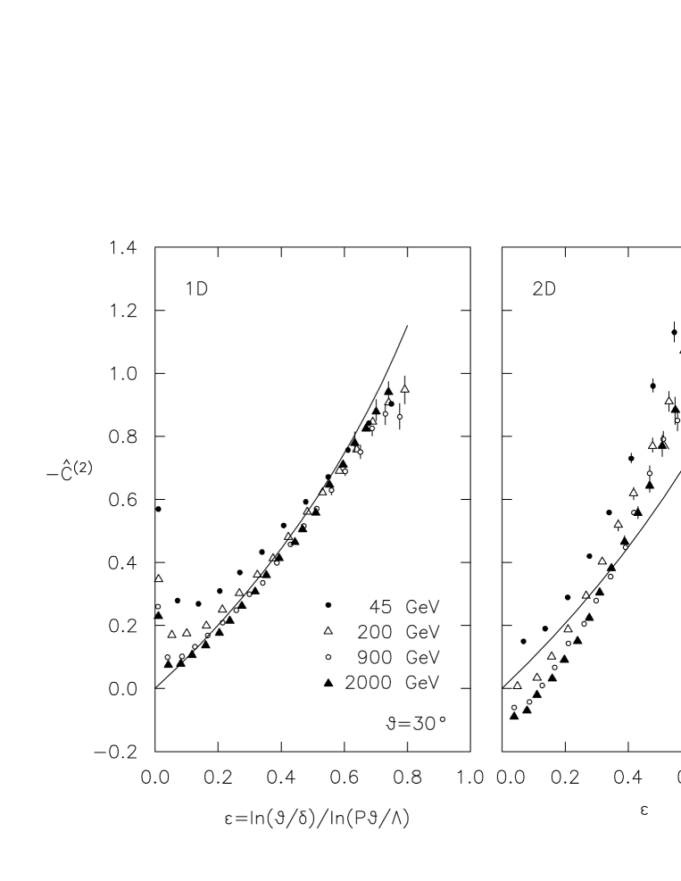
First we consider the correlation function $\hat{r}(\varepsilon)$ normalized by the full multiplicity in the forward cone. This quantity approaches at high energies a limiting distribution in $\varepsilon$, see Eq.(145),

$$-\frac{\ln\hat{r}(\varepsilon)}{2\sqrt{\ln\frac{P\Theta}{\Lambda}}}\simeq 2\beta(1-\frac{1}{2}\omega(\varepsilon,2))$$ (221)

where we dropped the contribution from the $\varepsilon$-independent prefactor. As can be seen from Fig. 7.1 the results from the parton MC nicely confirm the prediction of scaling in $\varepsilon$ in the energy interval considered and in the range of $\varepsilon\leq 0.6$. For larger $\varepsilon$ one observes a violation of scaling as expected from the influence of the cutoff $Q_{0}$ (see also the insert in the figure). The full curve represents the asymptotic limit of the correlation function (221). Here and in the following we adjust the absolute normalization of the curve to the data. Only the large leading terms in the exponent can be considered as reliably calculated in our present approach, the normalization is an effect of nonleading order and therefore may obtain large corrections. The dashed curve represents the prediction from the quark jet (162). If we used our calculated normalization the dashed curve would be shifted downwards by 0.1 unit.

Next we consider the same correlation in $\vartheta_{12}$, but with the differential normalization of Eq.(123). We would again expect a scaling in $\varepsilon$ for this quantity, however, see Fig. 7.2, the data do not approach the scaling limit, Eq.(147). The finite energy corrections derived for quark jets from Eq.(160), see Fig. 5.3a, shift the peak of the distribution towards smaller $\varepsilon$, as observed in the MC, but the energy dependence is predicted to be much weaker. The scaling violations in the MC are found most pronounced for large $\varepsilon$, i.e. small relative angles $\vartheta_{12}$. Apparently the disagreement comes from the normalizing function $d^{(2)}_{prod}(\vartheta_{12})$ in Eq.(123). This function is built from the 1-particle angular distribution $\rho^{(1)}(\vartheta)$ which for small angles becomes very sensitive to the orientation of the jet axis. This will be discussed further below in the last subsection together with a possibly improved definition of this quantity.

7.2 Multiplicity moments

In Fig. 7.3 we show the normalized cumulant and factorial moments in dependence of $\varepsilon$ (by variation of $\delta$ in (89)) for two primary energies and both dimensions $D=1,2$. The theoretical curves for $C^{(2)}$ are computed from Eq.(216). The description of the MC data improves with increasing energy. Again the normalization of the curves is adjusted. From our calculation in Sect. 6 we obtain for the $D=1$ moment at $\epsilon=0$, i.e. for the full forward cone of half opening $2\vartheta$, the result $C^{(2)}(0)=1/(3a(P\vartheta)c_{a})$ which yields 0.62 and 0.78 at 45 and 900 GeV resp. for gluon jets (times 9/4 for quark jets). This is larger than the exact DLA result $C^{(2)}=F^{(2)}-1=1/3$, see Eq.(119). Our larger values at $\varepsilon=0$ are due to the approximation $\delta\ll\vartheta$ in the calculations for our typically small angular intervals. The strong decrease of data at small $\varepsilon$ is therefore not reproduced by our calculation at the lower energies (see also Fig. 6.2). Furthermore it is known that the DLA overestimates the value of the global $F_{2}$ and that correct inclusion of energy-momentum conservation leads to a reduction of its value [35].

In the r.h.s. of Fig. 7.3 we show the factorial moments $(F^{(2)}=C^{(2)}+1)$. At high energies $C^{(2)}\sim F^{(2)}$ in the exponential accuracy of DLA. We have plotted our analytic results on $C^{(2)}$ moments also with the data for the $F^{(2)}$ moments. We observe that they fit actually better to the $F$-moments which indicates a peculiar cooperation of non-asymptotic effects.

At large $\varepsilon$ the size of the $D=1$ moments is underestimated. This may be related to our requirement $\vartheta_{12}<\delta$ in our integration over the ring.

The moments with $D=2$ deviate strongly from the predicted shape at large $\epsilon$. The origin of this behaviour is presumably the influence of the $Q_{0}$-cutoff at finite energies (see also the impact of an exact calculation for $r(\vartheta_{12})$ at large $\varepsilon$ in Fig. 5.2), also a sensitivity to the choice of the jet axis (see below) could play a role - differently to the symmetric 1D moments. The normalization calculated for $\varepsilon=0$, $C^{(2)}(0)=4/(3a(P\vartheta)c_{a})$ in Eq. (311) would yield moments considerably larger than the MC-data.

Next we test the universal behaviour of moments at high energies predicted from Eq.(216). In order to exhibit this universality we consider the quantity

$$\hat{C}^{(n)}={\ln[(\delta/\vartheta)^{D(n-1)}C^{(n)}]\over n\sqrt{\ln({P\vartheta\over\Lambda})}}$$ (222)

and in complete analogy the quantity $\hat{F}^{(n)}$. This quantity approaches for $\varepsilon$ fixed, $P\to\infty$ the scaling limit

$$-\hat{C}^{(n)} \simeq 2\beta(1-\omega(\varepsilon,n)/n)$$ (223)

$$\approx 2\beta(1-\sqrt{1-\varepsilon})$$ (224)

where the last expression is independent of $n$ and follows in leading $n$ approximation for $\omega$. In Fig. 7.4 we plot $-\hat{C}^{(2)}$ at different energies vs. $\varepsilon$ and the approach to the scaling limit Eq.(223) is nicely demonstrated. The 2D moments have about the same dependence on $\varepsilon$ at all energies although with an energy dependent normalization, but the dependence on $\varepsilon$ is steeper than expected from universality Eq.(223). In Fig. 7.5 we show the MC results on $\hat{F}^{(2)}$. The 1D moments show a rather nice scaling behaviour in $\varepsilon$ with the expected $\varepsilon$-dependence of Eq.(223) which sets in already at low energies.

Finally we consider the $n$-dependence of moments. Results of analytic calculations were shown already in Fig. 6.3. In the quantity $\hat{C}^{(n)}$ the leading $n$ dependence of $\omega(\varepsilon,n)\sim nf(\varepsilon)+O(1/n)$ is removed. The residual $n$-dependence is shown by the curves in Fig. 7.6. They are reproduced reasonably well by the MC data.

Remarkably, all angular correlations calculated here by the MC (except $r(\vartheta_{12})$) approach a scaling limit in $\varepsilon$ as predicted. Even very different quantities like $\hat{r}(\varepsilon)$ and the $D=1$ moments $C^{(2)},F^{(2)}$ - they are calculated for particles in different regions of phase space, also $\hat{r}$ is a differential, $C,F$ are integral quantities - approach the same asymptotic behaviour predicted by Eqs.(221,223), disregarding the normalization. An experimental verification of this prediction would be an interesting confirmation of the universalities occuring in the QCD parton cascade.

7.3 Hadronization

So far we have compared our analytic calculations with the MC results at the parton level to check the quality of our approximations. Next we investigate how the process of hadron formation modifies the results obtained at the parton level. For this purpose we apply the cluster model as incorporated in the HERWIG MC [16]. In fig. 7.7 we compare MC results at the parton and hadron level. There is good agreement in particular for small $\epsilon$ (large angles) but some discrepancy towards the small angle cutoff. The agreement further improves with increasing energy.

At sufficiently large angles the normalized quantities considered in this paper are infrared safe, i.e. become independent of the cutoff $Q_{0}$. It appears that in this kinematic regime the hadronization effects are negligable also, i.e. the model realizes local parton hadron duality. This is an interesting new criterion for the applicability of this phenomenological rule.

7.4 Limitations of the DLA

One important problem is the choice of the jet axis which should correspond to the primary parton direction in the DLA. This we have chosen to be the sphericity axis (in some cases we also tried the thrust axis without appreciable difference). Some quantities, like the angular distribution at small angles with respect to the axis, are quite sensitive to the precise direction of the axis in an event, whereas other, integral quantities, like the multiplicity in the forward cone with half angle $\Theta$ around the jet axis, are less sensitive to this choice. This problem is illustrated in Fig. 7.8 which shows the distribution of partons $\rho^{(1)}(\eta)$ in pseudorapidity $\eta=-\ln(\vartheta/2)$ with respect to the sphericity axis. Also shown is the DLA result - using either the exact form (41) or the high energy approximation (42) for $\rho^{(1)}(\vartheta)$ - which scales in $x=P\vartheta/\Lambda$ or $\ln x=\ln(2P/\Lambda)-\eta$. We see that this scaling property is strongly violated by the MC data, in particular for large $\eta\approx\eta_{max}$ or small angles $\vartheta$. Clearly, the jet axis defined in a multiparticle event does not coincide with the direction of the primary parton. Therefore the distribution $\rho^{(1)}(\vartheta)$ is not well defined at small angles.

This also explains the bad scaling properties of the correlation function $r(\vartheta_{12})$, Eq.(123), observed in Fig. 7.2. Namely, the normalizing function $d^{(2)}_{prod}(\vartheta_{12})$ is proportional to $\rho^{(1)}(\vartheta_{12})\bar{n}(\vartheta_{12})$, see Eq. (128), and therefore no good scaling properties can be expected for small $\vartheta_{12}$. On the other hand, the quantities $\hat{r}(\epsilon)$ and the $D=1$ moments depend on the jet axis only through the large angles $\Theta$ or $\vartheta$, furthermore there is a rotational symmetry, therefore these observables are stable against small fluctuations of the jet axis.

There is an interesting possibility to improve on this [21]. Instead of defining an observable with respect to a global jet axis one calculates this observable with respect to the directions of all particles in an event in turn, each one weighted by the respective particle’s energy. For the angular distribution, for example, one defines

$$\rho_{E}^{(1)}(\vartheta)=\int d^{3}k_{1}d^{3}k_{2}\frac{|k_{1}|}{W}\rho^{(2)}(k_{1},k_{2})\delta(\vartheta-\Theta_{k_{1}k_{2}})$$ (225)

This quantity is also shown in Fig. 7.8. As can be seen, the scale breaking is largely removed. In this paper we restrict ourselves to observables using the sphericity axis. It will be interesting to study the possible improvements using the modified definitions like (225) for our observables $r(\vartheta_{12})$ and also the $D=2$ moments to investigate the sensitivity to the jet axis. A further improvement would be the calculation of quantities like (225) within DLA (see ref. [21] for the azimuthal angle correlations). This would eliminate the global jet axis from both the theoretical and experimental analysis.

Another serious effect of the DLA is the neglect of the recoil. The energy-recoil can be taken into account in the so-called MLLA [4]. Its effect for moments has been studied in [22] and is found to be typically of the order of 10%. There is not yet any scheme available to include the angular recoil. Its significance can be recognized from studying $r(\vartheta_{12})$ in the full angular region $0\leq\vartheta_{12}\leq 2\Theta$. Note that in the DLA applied in this paper there is a peak near $\vartheta_{12}\approx 0$ but the correlation is minimal ($r=1$) for $\Theta\leq\vartheta_{12}\leq 2\Theta$ because of angular ordering. On the other hand the MC calculation yields a second peak near $\vartheta_{12}\simeq 2\Theta$ (not shown) of the same strength which is due to the recoiling primary parton. Therefore the inclusion of the angular recoil in the analytic calculations seems to be the most important problem for the more quantitative analysis of angular correlations.

8 Summary and concluding remarks

Beginning from a single principle, i.e. the master equation for the generating functional of the QCD cascade, we have derived a variety of predictions for angular correlations between partons. In particular we have calculated the distribution of the relative angle $\rho(\vartheta_{12})$, the fully differential two-body angular correlations $\Gamma(\Omega_{1},\Omega_{2})$ and subsequently also the general $n-$parton correlations. Multiplicity moments of general order in a restricted angular phase space were also computed. All calculations were done for constant and running $\alpha_{s}$ , and the correspondence between these results was always demonstrated. The double logarithmic approximation applied here provides the correct high energy limit. Some nonleading effects, namely the ones which are included in the master equation were also investigated.

This work summarizes and extends our earlier studies [11]-[14]. Some of the results on multiplicity moments were obtained also by other groups [21, 22, 23] as mentioned in the introduction.

An interesting aspect of the angular correlations considered here is their sensitivity to the soft gluon interference as the angular ordering prescription enters all calculations in an essential way. Indeed, in a recent study of polar angle correlations [36], using a quantity very similar to our $\rho(\vartheta_{12})$, a large effect from the angular ordering has been noted - unlike in the case of the azimuthal angle or momentum correlations.

Universal $\epsilon$ - scaling. We have studied in detail the emergence of the power dependence on the scale characteristic in the given process. Whenever the observable in question depends on the single scale only, then, in the high energy limit, it is a simple power of that scale. This is the case for the total multiplicity and factorial moments in a forward cone, and for the angular distribution, e.g. $\bar{n}\sim Q_{1}^{a(Q_{1})}$. For fixed $\alpha_{s}$ (constant anomalous dimension $a$) one obtains a power law in $Q_{1}$ whereas in case of running $\alpha_{s}$ the power law is violated by the scale dependence of $a(Q_{1})$.

For more complicated reactions, which in general depend on two or more independent scales, no straightforward power behaviour exists. We have found instead a scaling behaviour of a new type which applies universally to a large number of at first sight not related angular observables. In case of two scales $Q_{1},Q_{2}$, the distribution of the relative angle and the second cumulant moment in the sideway cone, for example, show the universal scaling behaviour

$$\rho\sim\exp{\left(\beta\sqrt{\ln Q_{1}}f(\epsilon)\right)},$$ (226)

where $f(\epsilon)$ is a calculable universal function of the ratio of the logarithm of the two scales $\epsilon={\ln{Q_{2}}\over\ln{Q_{1}}}$. Up to some simple kinematic factors, the scaling function $f(\epsilon)$ is the same for both quantities and analogous functions in $\epsilon$ occur for the higher correlations. The general result, Eq.(226), implies that the simple power dependence on only one scale can be recovered in the ”diagonal” scaling limit for fixed $\epsilon$, e.g. when $Q_{1},Q_{2}\rightarrow\infty,Q_{1}=Q_{2}^{\epsilon}$. Indeed then Eq.(226) reduces to

$$\rho\sim Q_{1}^{a(Q_{1})f(\epsilon)}$$ (227)

with the anomalous dimensions depending on $\epsilon$. The same phenomenon was found for the single particle momentum distribution, Eq.(58), which also depends essentially on two scales.

The “$\epsilon$-scaling”, Eq.(226), has interesting experimental consequences. The observable quantity $f(\epsilon)\sim\ln\rho/\sqrt{\ln Q_{1}}$ should depend on the three relevant variables (for example $\vartheta,\delta,P$) only through the single variable $\epsilon$, i.e. two variables are redundant. Preliminary results from LEP [37] have verified recently this scaling prediction for the polar angle correlation [12]. The $\epsilon$-scaling holds approximately for the opening angles $\Theta$ in the range $30^{o}<\Theta<60^{o}$.

Intermittency and fractal structure. Results of this work have a direct application to the intermittency studies which have recently attracted a lot of attention. This property of the parton cascade is obtained from the general formula (226) in the limit of small $\epsilon$, i.e. sufficiently large opening angles, in the linear approximation of $f(\epsilon)$. The suitably normalized observables then behave like $r\sim Q_{2}^{ca(Q_{1})}$, i.e. there is a power law in one scale $Q_{2}$ (say $\vartheta/\delta$) if the other scale $Q_{1}$ (say $P\vartheta$) is kept fixed. So the perturbative cascade is intermittent in the appropriate angular variables and intermittency exponents are available analytically, c.f. Eq.(216). For fixed $\alpha_{s}$ the power behaviour for the angular correlations is actually approached in the full angular region for high energies.

This power dependence can be related to the selfsimilar structure of the partonic branching process. One can assign a fractal dimension $D_{n}$ to the normalized multiplicity moments and this is found to be given in terms of the anomalous dimension of total multiplicity $a=\gamma_{0}=\sqrt{6\alpha_{s}/\pi}$, see Eq. (220).

Monte Carlo tests. We have also confronted the analytical predictions with Monte Carlo simulations which don’t have many of the limitations of the double logarithmic approximation. The results are rather satisfactory. One indeed sees the approximate $\epsilon$-scaling (226) and the shape of the scaling function is approached with increasing energy. The factorial moments are closer to the asymptotic limit than the cumulant moments. In the small $\epsilon$ region the correlation functions and moments are independent of the $p_{T}$ cutoff $Q_{0}$. In this region we find the hadronization effects negligable in the Monte Carlo (HERWIG) calculations. On the other hand deviations occur for particles with small angular separation.

To conclude, there exists a rich spectrum of analytic predictions from the perturbative QCD for multiparton correlations. The double logarithmic approximation provides the leading order predictions applicable quantitatively at very high energies ($\sim 1$ TeV) but some interesting experimental tests of the theory in its relatively unexplored regime are suggested already at present energies.

Appendix A

In this Appendix we shall derive asymptotic form of the solution Eq.(86). Consider first the case of constant $\alpha_{s}$ . This will allow to rederive the results obtained also directly from the correlation function, cf. Eq.(304), and will provide some orientation about the relevant range of variables contributing to the integrals in question. Inserting moments, Eq.(54), into Eq.(86) gives for the leading term

$$\overline{h}_{n}(\delta,\vartheta,P) = \int_{\gamma}{ds\over 2\pi i}{\sqrt{s^{2}+4a^{2}}+s\over 2\sqrt{s^{2}+4a^{2}}}$$

$$\int_{Q_{0}/\delta}^{P}{dK\over K}\exp{\left[{1\over 2}\ln{P\over K}(\sqrt{s^{2}+4a^{2}}-s)\right]}$$

$$\int_{\delta}^{\vartheta}{d\Psi\over\Psi}\exp{\left[{1\over 2}\ln{\vartheta\over\Psi}(\sqrt{s^{2}+4a^{2}}+s)\right]}d_{n}(K,\delta),$$

with the source term $d_{n}(K,\delta)={\cal D}_{n}(K\delta/Q_{0})^{na}$. After changing the variable in the inner integration to $u=\ln{(\vartheta/\Psi)}$, we can extend the upper limit to the infinity. If the contour $\gamma$ is properly chosen this does not affect the leading behaviour of the result. One obtains

$$\overline{h}_{n}(\delta,\vartheta,P)={\cal D}_{n}\int_{\gamma}{ds\over 2\pi i}{1\over\sqrt{s^{2}+4a^{2}}}$$

$$\int_{Q_{0}/\delta}^{P}{dK\over K}\exp{\left[{1\over 2}\ln{P\over K}(\sqrt{s^{2}+4a^{2}}-s)\right]}\left({K\delta\over Q_{0}}\right)^{na},$$

Similar procedure for the $K$ integration gives the pole in $s$

$$\overline{h}_{n}(\delta,\vartheta,P) = {\cal D}_{n}\left({P\delta\over Q_{0}}\right)^{na}\int_{\gamma}{ds\over 2\pi i}{1\over\sqrt{s^{2}+4a^{2}}}{2\over(\sqrt{s^{2}+4s^{2}}-2s)-na}$$

$$\exp{\left[{1\over 2}\ln{\vartheta\over\delta}(\sqrt{s^{2}+4a^{2}}+s)\right]},$$

This pole saturates the contour integral giving finally

$$\overline{h}_{n}(\delta,\vartheta,P)={\cal D}_{n}\left({\delta\over\kappa}\right)^{na}\left({\vartheta\over\delta}\right)^{\frac{a}{n}},$$ (231)

where $\kappa=Q_{0}/P$. Normalization ${\cal D}_{n}$ follows from Eq.(204). We obtain

$${\cal D}_{n}={aF_{n}\over\pi 2^{n+1}n},$$ (232)

with $F_{n}\equiv\lim_{x\rightarrow\infty}f_{n}(x)/n_{tot}(x)^{n}$. With $F_{2}=4/3$, cf. (119), Eq.(231) reproduces Eq.(304) for $n=2$.

Runnung $\alpha_{s}$ . Similarly to the previous case the saddle point $s^{*}$ in Eq.(87) scales as the coupling constant hence $s^{*}\sim 1/\sqrt{\ln{P}}$. Therefore it is sufficient to use the appropriate asymptotic forms of the confluent hypergeometric functions. They can be derived from the well known integral representations of the solutions of the conflunt hypergeometric equation [38]. We obtain

$$\lim_{a\rightarrow+\infty,z\rightarrow+\infty,b=const}F(a,b,z) = {1\over\sqrt{2\pi}}({z\Delta\over 4})^{1-b\over 2}(z^{2}+z\Delta)^{-{1\over 4}}$$ (233)

$$\exp{\left[{1\over 2}(\sqrt{z^{2}+z\Delta}+z)\right]} \exp{\left[{\Delta\over 2}\ln{(\sqrt{z\over\Delta}+\sqrt{{z\over\Delta}+1})}\right]}.$$

$$\lim_{a\rightarrow\infty,z\rightarrow\infty,b=const}\Phi(a,b,z) = z^{{1\over 4}-{b\over 2}}(z+\Delta)^{-{1\over 4}}e^{\Delta\over 4}$$ (234)

$$\exp{\left[-{1\over 2}(\sqrt{z(z+\Delta)}-z)\right]} \exp{\left[-{\Delta\over 2}\ln{\sqrt{z}+\sqrt{z+\Delta}\over 2}\right]}.$$

where $\Delta=4a-2b$. This implies the following asymptotics for the ${\cal A}$ and ${\cal F}$ functions required in Eq.(87).

$${\cal F}(s,x)\simeq \sqrt{s\over 2\pi\beta^{2}p_{x}} e^{{x\over 2}g_{-}(s,x)}\exp{\left[{2\beta^{2}\over s}\ln{({\sqrt{x}\over 2\beta}g_{+}(s,x)})\right]},$$ (235)

$${\cal A}(s,\lambda)\simeq \sqrt{2\pi\beta^{2}\over s}{1+p_{\lambda}\over 2\sqrt{p_{\lambda}}} e^{-{\lambda\over 2}g_{-}(s,\lambda)}\exp{\left[-{2\beta^{2}\over s}\ln{({\sqrt{\lambda}\over 2\beta}g_{+}(s,\lambda)})\right]},$$ (236)

$$g_{\pm}(s,x) = \sqrt{s^{2}+4\beta^{2}/x}\pm s,$$ (237)

where $p_{\tau}\equiv\sqrt{1+4{\beta^{2}\over s^{2}\tau}}.$ Now Eq.(87) can be rewritten as

$$\overline{h}_{n}(\delta,\vartheta,P)=\int_{\gamma}\exp{(s\ln{\vartheta\over\delta})}{\cal F}(s,\ln{P\vartheta\over\Lambda})\overline{u}_{n}(s)\exp{w_{n}(s,\ln{P\delta\over\Lambda})}{ds\over 2\pi i},$$ (238)

where

$$\overline{u}_{n}(s)\exp{w_{n}(s,\ln{P\delta\over\Lambda})}= \int_{\ln{Q_{0}/\Lambda}}^{\ln{P\delta/\Lambda}}d\sigma u_{n}(s,\sigma)\exp{v_{n}(s,\sigma)},$$ (239)

$$v_{n}(s,\sigma)= -{\sigma\over 2}g_{-}(s,\sigma)- {2\beta^{2}\over s}\ln{({\sqrt{\sigma}\over 2\beta}g_{+}(s,\sigma))}+2n\beta\sqrt{\sigma},$$

$$u_{n}(s,\sigma)= \sqrt{2\pi\beta^{2}\over s} {1+p_{\sigma}\over 2\sqrt{p_{\sigma}}}{\cal D}_{n},$$ (240)

and the prefactor resulting from the inhomogenous term $d_{n}(\sigma)=$ ${\cal D}_{n}\exp{(2n\beta\sqrt{\sigma)}}$ follows from Eqs.(204,120) and (36).

$${\cal D}_{n}={a(\sigma)F_{n}\over 2\pi n}\left({f\over 2\sqrt{a(\sigma)}}\right)^{n}.$$ (241)

Saddle point condition for the $\sigma$ integration $\partial_{\sigma}v_{n}(\sigma,s)=0$ gives

$$g_{-}(s,\sigma)={2n\beta\over\sqrt{\sigma}},$$ (242)

which has the solution

$$\sigma^{\star}={\beta^{2}(1-n^{2})^{2}\over s^{2}n^{2}}.$$ (243)

At the saddle

$$v_{n}(s,\sigma^{\star})={\beta^{2}\over s}(1-n^{2})+{2\beta^{2}\over s}\ln{n}\equiv w_{n}(s).$$ (244)

which is independent of the $P\delta$ and corresponds to the insensitivity of the leading contribution to the integral (239) to the upper limit of integration. The prefactor reads

$$\overline{u}_{n}(s)=\sqrt{2\pi\over\ddot{v}_{n}(\sigma^{\star})}u_{n}(\sigma^{\star})={\beta^{2}F_{n}\over s^{2}n}\sqrt{2(n^{2}-1)}\left({f\over 2}\right)^{1-{n\over 2}}a(\sigma^{\star})^{1-{n\over 2}}.$$ (245)

We now follow similar procedure for the $s$ integral. Writing

$$h_{n}(\delta,\vartheta,P)\simeq\int_{\gamma}U_{n}(s)\exp{W_{n}(s,L,l)}{ds\over 2\pi i},$$ (246)

we have from (235,236,238,244) $L=\ln{(P\vartheta/\Lambda)},l=\ln{(P\delta/\Lambda)}$

$$W_{n}(s,L,l) = s(L-l)+$$ (247)

$${1\over 2}Lg_{-}(s,L) + {2\beta^{2}\over s}\ln{[{n\sqrt{L}\over 2\beta}g_{+}(s,L)]}-{\beta^{2}\over s}(n^{2}-1),$$ (248)

and

$$U_{n}(s,L)=\sqrt{s\over 2\pi\beta^{2}p_{L}}\overline{u}_{n}(s).$$ (249)

Saddle point condition, $\partial_{s}W_{n}(s,L,l)=0$, gives after some algebra Eq.(92) with $z=s\sqrt{L}/\beta$ . In addition Eq.(248) can be simplified at the saddle point reducing finally to

$$W_{n}(s^{\star},L,l)=2\beta L\omega(\epsilon,n),$$ (250)

and the overall prefactor

$$\Pi_{n}(s^{*})={1\over\sqrt{2\pi W^{{}^{\prime\prime}}_{n}(s^{\star})}}U_{n}(s^{\star})\equiv{\cal D}_{n}{\cal P}_{n},$$ (251)

which after some algebra gives Eq.(95) for ${\cal P}_{n}$ . It is easy to check that in the constant $\alpha_{s}$ limit our Eq.(88) reduces to the result (231) derived by the exact integration of the resolvent representation (Appendix A).

Appendix B

In this Appendix we shall derive the constant $\alpha_{s}$ limit of the energy moments, Eq.(49). This is done by leting $\beta,\lambda\rightarrow\infty$ while keeping the ratio $\beta^{2}/\lambda\equiv a$ constant. In this process the first parameter and the independent variable of the hypergeometric confluent functions become large. Appropriate asymptotic forms of these functions are derived in Appendix A. Using Eqs.(Appendix A) and (Appendix A) one obtains for the ingredients of the first part of Eq.(49)

$$\Phi(\alpha-1,1,s\lambda)\simeq(s\lambda)^{-1/4}(s\lambda+4\beta^{2}/s-2)^{-1/4}\exp{(\beta^{2}/s-1/2)}$$

$$\exp{\left[-{1\over 2}\left(\sqrt{s\lambda(s\lambda+4\beta^{2}/s-2)}-s\lambda\right)\right]}$$

$$\exp{\left[-\left({2\beta^{2}\over s}-1\right)\ln{\sqrt{s\lambda}+\sqrt{s\lambda+4\beta^{2}/s-2}\over 2}\right]},$$

$$F(\alpha,2,s(X+\lambda))\simeq{1\over\beta(X+\lambda)\sqrt{2\pi s}}\left(1+{4\beta^{2}\over s^{2}(X+\lambda)}\right)^{-1/4}\exp{\left({\beta^{2}\over s}\ln{s^{2}(X+\lambda)\over 4\beta^{2}}\right)}$$

$$\exp{\left[{s(X+\lambda)\over 2}\left(\sqrt{1+{4\beta^{2}\over s^{2}(X+\lambda)}}+1\right)\right]}\exp{\left[{2\beta^{2}\over s}\ln{\left(1+\sqrt{1+{4\beta^{2}\over s^{2}(X+\lambda)}}\right)}\right]}.$$

All symbols are as in Eq.(49) except that $n$ was replaced by the continuous variable $s$. Constant $\alpha_{s}$ limit is performed at fixed values of the kinematical variables. In particular, $X/\lambda<<1$ and $s\lambda>>1$ in this limit. Expanding above expressions and keeping track of the $O(\lambda)$ and $O(1)$ terms in the exponents we obtain

$$\Phi(\alpha-1,1,s\lambda)\simeq{s+\sqrt{s^{2}+4a^{2}}\over 2\sqrt{s\sqrt{s^{2}+4a^{2}}}}\exp{(\beta^{2}/s-1/2)}$$

$$\exp{\left(-{\lambda\over 2}(\sqrt{s^{2}+4a^{2}}-s)\right)}\exp{\left(s\over 2\sqrt{s^{2}+4a^{2}}\right)}\exp{\left(-{\beta^{2}\over s}\ln{(s\lambda)}\right)}$$

$$\exp{\left(-{2\beta^{2}\over s}\ln{s+\sqrt{s^{2}+4a^{2}}\over 2s}\right)}\exp{\left(2a^{2}\over\sqrt{s^{2}+4a^{2}}(s+\sqrt{s^{2}+4a^{2}})\right)},$$

$$F(\alpha,2,s(X+\lambda))\simeq{1\over\beta(X+\lambda)\sqrt{2\pi\sqrt{s^{2}+4a^{2}}}}\exp{\left(-{a^{2}X\over\sqrt{s^{2}+4a^{2}}}\right)}$$

$$\exp{\left({X+\lambda\over 2}(\sqrt{s^{2}+4a^{2}}+s)\right)}\exp{\left({\beta^{2}\over s}\ln{s^{2}\lambda\over\beta^{2}}\right)}\exp{\left({a^{2}X\over s}\right)}$$

$$\exp{\left({2\beta^{2}\over s}\ln{s+\sqrt{s^{2}+4a^{2}}\over 2s}\right)}\exp{\left(-{4a^{4}X\over s\sqrt{s^{2}+4a^{2}}(s+\sqrt{s^{2}+4a^{2}})}\right)}.$$

Where we have already replaced the $O(1)$ ratio $\beta^{2}/\lambda$ by $a$. Finally, inserting these expressions into Eq.(49) and using Stirling formula for the gamma function, we see that the divergent, leading terms canel and the first nonleading corrections give the finite result which reproduces the first part of Eq.(54). Second part is obtained in the analogous way from the second term of Eq.(49).

Appendix C

We shall discuss here some details of the derivation of the simplified resolvent representation, Eq.(86). First we will derive Eq.(85). To this end recall the resolvent solution for the two dimensional inclusive density, Eq.(77). Performing the steps outlined there one obtains with the running $\alpha_{s}$

$$\rho(k,\vartheta,P)=a^{2}(k,\vartheta)+\int_{k}^{P}\frac{dK}{K}\int_{Q_{0}/k}^{\vartheta}\frac{d\Psi}{\Psi}R\left({P\over K},{\vartheta\over\Psi},{K\Psi\over\Lambda}\right)a^{2}(K,\Psi).$$ (254)

Formula for the momentum distribution follows from Eq.(254) upon the angular integration. Changing orders of the $\vartheta$ and $\Psi$ integrations, recalling the definition (following Eq.(79)) of $\overline{R}$ and using the substitution rules (84) gives Eq.(85). In the reduced variables $x=\ln{\vartheta\over\delta},t=\ln{P\delta\over Q_{0}},z=\ln{\Psi\over\delta},\tau=\ln{K\delta\over Q_{0}},\lambda=\ln{Q_{0}\over\Lambda}$ it reads

$$h_{n}(x,t,\lambda)=d_{n}(t+\lambda)+\int_{0}^{x}dz\int_{0}^{t}d\tau\overline{R}(x-z,t-\tau,z+\tau+\lambda)\partial_{\tau}d_{n}(\tau+\lambda).$$ (255)

Integrating by parts and noting that $d$ is independent of $z$ we obtain

$$h_{n}(x,t,\lambda)=d_{n}(t+\lambda)+\int_{0}^{t}d\tau\tilde{R}(x,t-\tau,\tau+\lambda)d_{n}(\tau+\lambda).$$ (256)

where we have introduced

$$\tilde{R}(x,t-\tau,\tau+\lambda)=\int_{0}^{x}\partial_{t}\overline{R}(x-z,t-\tau,z+\tau+\lambda).$$ (257)

Because $\overline{R}$ has the Laplace representation, Eq.(87), which is dominated by $s\sim O(1/\ln{P\over Q_{0}})$, one can set to the leading order $\partial_{1}\overline{R}(x_{1},x_{2},\lambda)=\partial_{2}\overline{R}(x_{1},x_{2},\lambda)$. Therefore finally

$$\tilde{R}(x,t-\tau,\tau+\lambda)=\int_{0}^{x}dz\partial_{x}\overline{R}(x-z,t-\tau,z+\tau+\lambda)=\overline{R}(x,t-\tau,\tau+\lambda),$$ (258)

since the contribution from the upper limit $z=x$ is negligible . This concludes the proof of Eq.(86) which can be also simply summarized as the dominance of the lower limit in the $\Psi$ integration in Eq.(85).

Appendix D

In this Appendix we shall derive the asymptotic behaviour, Eq.(120), of the total factorial moments, and the recursive relation (121) for constant $\alpha_{s}$ . First, we simplify the resolvent solution for $f_{n}(X)$. Changing the integration variables $Z$ and $\zeta$ in Eq.(70) to $t=Z+\Xi$ and $v=Z+\zeta$ and interchanging the order of $t$ and $v$ integrals one can perform the $t$ integral to obtain

$$f_{n}(X)=b_{n}(X)+a\int_{0}^{X}\sinh{(a(X-v))}b_{n}(v)dv,$$ (259)

with $X=Y+\Xi=\ln{(P\Theta/Q_{0})}$. We now prove Eq.(120) by induction. For $n=2$,

$$b_{2}(X)=<n>^{2}\simeq B_{2}\exp{(2aX)}/2^{2}.$$ (260)

Assume now that

$$b_{n}(X)=B_{n}\left({1\over 2}e^{aX}\right)^{n}.$$ (261)

Inserting (261) into (259) one easily verifies (120) with

$$F_{n}={n^{2}\over n^{2}-1}B_{n}.$$ (262)

Since $b_{n}(X)$ is built recursively from the products of moments of lower order (for example $b_{3}(X)=<n>^{3}+3<n>(f_{2}(X)-b_{2}(X))$) with the same combined anomalous dimension, the form (261) follows. This completes the inductive proof of Eq.(120).

In order to derive now the recurrence relation (121) we rewrite the master equation, Eq.(7), for the generating function of the global moments, i.e. we set $u(K)\equiv u$. In the high energy limit the nested terms are negligible which amounts to puting $u=1$ in the exponent of Eq.(7). With these simplifications Eq.(7) reads

$$Z_{P}(u)=\exp{(\int d^{3}K{\cal M}_{P}(K)(Z_{K}(u)-1))}.$$ (263)

Differentiating $n$ times one obtains

$$f_{n}(X)=\sum_{k=1}^{n-1}{n-1\choose k}f_{k}(X)g_{n-k}(X)+g_{n}(X),$$ (264)

where we have introduced the cumulant moments

$$g_{m}(X)\equiv\int d^{3}K{\cal M}_{P}(K)Z^{(m)}_{K}(u)_{|u=1}=f_{m}(X)-b_{m}(X).$$ (265)

Using the last equality and Eqs(120,261) together with Eq.(262) to eliminate $g_{m}$ in favour of $f_{m}$ gives the recursion Eq.(121).

Appendix E

In this Appendix we shall derive the series representation Eq.(135) for the distribution of the relative angle $\vartheta_{12}$ for constant $\alpha_{s}$ . The contributions from the product and nested terms will be calculated separately.
A. Product term. Inserting Eqs.(131) and (132) into Eq.(130) and expanding in powers of $a$ one obtains upon integration over $\Psi$ ($\kappa=Q_{0}/P$)

$$\gamma_{prod} \equiv \rho^{(2)}_{prod}(\vartheta_{12})-d_{prod}^{(2)}(\vartheta_{12})$$

$$= {2a^{2}\over\vartheta_{12}}\sum_{r=0}^{\infty}{a^{2r+1}\over r!(r+1)!}\ln^{r+1}{\left(\Theta\over\vartheta_{12}\right)}f_{r}\left({\vartheta\over\kappa}\right),$$

with

$$f_{r}(y)=\sum_{m=0}^{\infty}{4^{m}-1\over(2m+1)!}\int_{0}^{y}(y-z)^{r}z^{2m+1}dz.$$ (267)

Integration over $z$ is proportional to the Euler beta function
$B(\mu,\nu)=\int_{0}^{1}t^{\mu-1}(1-t)^{\nu-1}$. Changing the orders of the $r$ and $m$ summations we obtain

$$\gamma_{prod}={2a\over\vartheta_{12}}\sum_{m=0}^{\infty}(4^{m}-1)\left\{\overline{y}^{m+1/2}I_{2m+1}(z)-{(a\ln{\vartheta/\kappa})^{2m+1}\over(2m+1)!}\right\}.$$ (268)

Where $\overline{y}=y^{2}/4$ and $y$ and $z$ are defined below Eq.(135). The second term in the curly bracket gives after summation the inhomogenous term $d_{prod}$, therefore the inclusive density itself is given by the first term only.
B. Nested term. Calculation of this contribution is entirely analogous to the previous one. After expanding $d_{nest}$, Eq.(133) and the resolvent (131) one is left with elementary integrals. Final result for the nested part reads

$$\rho^{(2)}_{nest}(\vartheta_{12})={2a\over\vartheta_{12}}\left(\sum_{m=0}^{\infty}\overline{y}^{m+1/2}I_{2m+1}(z)-\sinh{(a\ln(\vartheta_{12}/\kappa))}\right).$$ (269)

Adding both contributions gives the result (135).

Appendix F

In this Appendix we integrate the formula, Eq.(135) to obtain the total factorial moment $f_{2}$ as given by Eq.(119). Integration of the second term in (135) is trivial hence we write

$$\int_{\kappa}^{\Theta}d\vartheta_{12}\rho^{(2)}(\vartheta_{12},P,\Theta)=J\left(a\ln\left({\Theta\over\kappa}\right)\right)-2\left(\cosh\left(\ln{\Theta\over\kappa}\right)-1\right).$$ (270)

with $J(aX),X=\ln{(\Theta/\kappa)}$ defined as the integral of the first part of Eq.(135). Expanding modified Bessel functions one obtains

$$J(aX) = \sum_{m=0}^{\infty}\sum_{k=0}^{\infty}{2^{2m+1}a^{2m+2k+2}\over k!(k+2m+1)!}\int_{0}^{X}t^{2m+k+1}(X-t)^{k}dt$$

$$= \sum_{m=0}^{\infty}2^{2m+1}\sum_{k=0}^{\infty}{(aX)^{2m+2k+2}\over(2m+2k+2)!},$$

which can be resummed

$$J(Y) = \sum_{l=0}^{\infty}{Y^{2l+2}\over(2l+2)!}\sum_{m=0}^{l}2^{2m+1}$$

$$= {2\over 3}\left(\cosh{(2Y)}-\cosh{(Y)}\right).$$

Inserting (Appendix F) into (270) gives

$$\int_{\kappa}^{\Theta}\rho^{(2)}(\vartheta_{12})d\vartheta_{12}={4\over 3}\left(\cosh(aX)-1\right)^{2},$$ (273)

in agreement with Eq.(119).

Appendix G

We derive here the asymptotic form, Eq.(136), of the correlation function (135) at high energies $\kappa=Q_{0}/P\to 0$. In this limit

$$y=2\sqrt{{\ln{(\vartheta_{12}/\kappa)}\over\ln{(\Theta/\vartheta_{12})}}}\to\infty,\;\;\;z=2a\sqrt{\ln{(\vartheta_{12}/\kappa)}\ln{(\Theta/\vartheta_{12})}}\to\infty,$$ (274)

with

$$z/y=a\ln{(\Theta/\vartheta_{12})}\equiv\sigma^{2}/2=const.$$ (275)

Using the sum rule,

$$\sum_{k=0}^{\infty}y^{k}I_{\nu+k}(z)=z^{-\nu}e^{yz/2}\int_{0}^{z}e^{-y\tau^{2}/(2z)}I_{\nu-1}(\tau)\tau^{-\nu}d\tau,\;\;\;\nu>0,$$ (276)

one can rewrite the sum in Eq.(135) as

$$\rho^{(2)}(\vartheta_{12},P,\Theta)={a\over\sigma^{2}\vartheta_{12}}\left(e^{zy/2}\int_{0}^{z}e^{-\tau^{2}/\sigma^{2}}I_{0}(\tau)\tau d\tau+e^{-zy/2}\int_{0}^{z}e^{\tau^{2}/\sigma^{2}}I_{0}(\tau)\tau d\tau\right),$$ (277)

with the first term $O((\vartheta_{12}/\kappa)^{2a})$ dominating the high energy behaviour. We have neglected the terms $O((\vartheta_{12}/\kappa)^{a})$. Since the integrand in the leading term is well behaved at large $\tau$, we can extract the large $P$ limit by setting the upper bound to infinity. This gives

$$\rho^{(2)}(\vartheta_{12},P,\Theta)={a\over\vartheta_{12}}\left({\vartheta_{12}\over\kappa}\right)^{2a}\int_{0}^{\infty}e^{-u^{2}}I_{0}(\sigma u)udu,$$ (278)

which can be integrated exactly to give finally

$$\rho^{(2)}(\vartheta_{12},P,\Theta)={a\over 2\vartheta_{12}}\left({\vartheta_{12}\over\kappa}\right)^{2a}e^{\sigma^{2}/4}.$$ (279)

This is identical with Eq.(136) after taking into account Eq.(275).

Appendix H

In this Appendix we shall perform several consistency tests of our results for the two-parton correlations.

First, we show that the form, Eq.(164), of the fully differential connected angular correlation is consistent with the Eq.(130) for the correlation in the relative angle. It suffices to show this compatibility for the connected parts only, since the relation between the direct terms was already established (cf. Eqs (127) and (132) ). To this end we define

$$\Gamma^{(2)}(\vartheta_{12})=\int d\Omega_{1}d\Omega_{2}\delta(\vartheta_{12}-\Theta_{k_{1}k_{2}})\Gamma^{(2)}(\Omega_{1},\Omega_{2}),$$ (280)

with $\Gamma^{(2)}(\Omega_{1},\Omega_{2})$ given by Eq.(164). Due to the symmetry between partons if is sufficient to analyse only the first term ($\Gamma_{1}$, say) in Eq.(164). Choosing the polar coordinates of the $d\Omega_{2}$ integration relative to the direction of the momentum of the first parton one obtains

$$\Gamma^{(2)}(\vartheta_{12})=2\int d\Omega_{1}\int\Theta_{k_{1}k_{2}}d\Theta_{k_{1}k_{2}}d\phi_{12}\Gamma_{1}^{(2)}(\Omega_{1},\Omega_{12})\delta(\vartheta_{12}-\Theta_{k_{1}k_{2}}),$$ (281)

which gives after performing integrations over $\Theta_{Kk_{1}}$ (in (164)), $\Theta_{n_{1}n_{2}}$ and $\phi_{12}$

$$\Gamma^{(2)}(\vartheta_{12}) = {2a^{3}\over\vartheta_{12}}\int_{Q_{0}/\vartheta_{12}}^{\Theta}{dK\over K}\left(\cosh{(a\ln(K\vartheta_{12}/Q_{0}))}-1\right)$$

$$\sinh{(a\ln(K\vartheta_{12}/Q_{0}))}\int_{\vartheta_{12}}^{\Theta}I({P\over K},{\Theta_{Pk_{1}}\over\vartheta_{12}}){d\Theta_{Pk_{1}}\over\Theta_{Pk_{1}}}.$$

This is identical with the resolvent solution (130) after changing the integration variable $\Theta_{Pk_{1}}$ to $\Psi=\Theta\vartheta_{12}/\Theta_{Pk_{1}}$.

As a second consistency check we integrate the cumulant correlation $\Gamma^{(2)}(\Omega_{1},\Omega_{2})$ up to the multiplicity moment $f_{2}$ for the full forward cone which is known [2] [4] to be $f_{2}/\bar{n}^{2}=4/3$, cf. Eq.(121), with either $\rho^{(2)}(\vartheta_{12})$ or $h^{(2)}(\Omega,\delta)$ and $c^{(2)}(\vartheta,\delta)$ as intermediate results.

In the first case we derive the cumulant correlation in the relative angle by integrating Eq.(166). One obtains

$$\Gamma^{(2)}(\vartheta_{12}) = \int d\Omega_{1}d\Omega_{2}\delta(\vartheta_{12}-\Theta_{k_{1},k_{2}})\Gamma^{(2)}(\Omega_{1},\Omega_{2})$$ (283)

$$= {1\over 8}({a\over 2\pi})^{2}\int^{\Theta}_{\vartheta_{12}}{2\pi d\vartheta_{1}\over\vartheta_{1}}{1\over\vartheta_{12}}({\vartheta_{12}\over\kappa})^{2a}({\vartheta_{1}\over\vartheta_{12}})^{a\over 2}+(1\leftrightarrow 2)$$

$$= {a\over 2\vartheta_{12}}({\vartheta_{12}\over\kappa})^{2a}[({\Theta\over\vartheta_{12}})^{a\over 2}-1].$$

Here we used again the pole approximation with the same results for both terms. With the results Eqs.(283,136) for $\rho^{(2)}(\vartheta_{12})$ and $d^{(2)}_{prod}(\vartheta_{12})$ we recover the relation (4) $\Gamma^{(2)}(\vartheta_{12})=\rho^{(2)}(\vartheta_{12})-d^{(2)}_{prod}(\vartheta_{12})$.

We can now calculate the multiplicity moment $f_{2}(\delta,\Theta)$ in a cone of half opening $\delta$ averaged over the forward cone $\Theta$ and the corresponding normalisation $\bar{n}^{2}(\delta,\Theta)$

$$f_{2}(\delta,\Theta)=\int^{\delta}_{\kappa}d\vartheta_{12}\rho^{(2)}(\vartheta_{12})\simeq{1\over 3}({\delta\over\kappa})^{2a}({\Theta\over\delta})^{a\over 2},$$ (284)

$$\bar{n}^{2}(\delta,\Theta)=\int^{\delta}_{\kappa}d\vartheta_{12}d^{(2)}_{prod}(\vartheta_{12})\simeq{1\over 4}({\delta\over\kappa})^{2a},$$ (285)

where the approximation is for $\delta\gg\kappa$. For the normalised moment we then obtain $F_{2}(\delta,\Theta)\simeq{4\over 3}({\Theta\over\delta})^{a\over 2}$ . This reproduces $F_{2}={4\over 3}$ in the full forward cone $(\delta\to\Theta)$. So we find here that the density $\rho^{(2)}(\vartheta_{12})$ and not the cumulant correlation $\Gamma^{(2)}(\vartheta_{12})$ follows a power law, although the difference between both quantities disappears for $\vartheta_{12}\ll\Theta$.

In the second case we note that the cumulant moments $h^{(2)}(\Omega,\delta)$ and $c^{(2)}(\Omega,\delta)$ derived from $\Gamma^{(2)}(\Omega_{1},\Omega_{2})$ are power behaved, cf. Eqs.(304,306), and not the factorial moments. To check the consistency with the previous results we calculate in analogy to Eqs.(284,285) the cumulant moment in cone $\delta$ averaged over the full cone $\Theta$.

$$c^{(2)}(\delta,\Theta)=\int^{\delta}_{\kappa}d\Omega h^{(2)}(\Omega,\vartheta)+\int^{\Theta}_{\delta}d\Omega h^{(2)}(\Omega,\delta),$$ (286)

The first term appears because of the requirement $\delta\leq\vartheta$. Using our result (304) for $h^{(2)}(\Omega,\delta)$ we obtain for $\delta\gg\kappa$

$$c^{(2)}(\delta,\Theta)\simeq{1\over 4}({\delta\over\kappa})^{2a}[{4\over 3}({\Theta\over\delta})^{a\over 2}-1].$$ (287)

With the normalisation (285) and the relations (4) we find again the consistency with the previous result on $f^{(2)}(\delta,\Theta)$ in (284), and therefore the correct integration to the full cone with $F_{2}={4\over 3}$.

Appendix I

Here we discuss the derivation of Eq.(175) for $\Gamma^{(n)}_{P}$ for general order $n$. First we have to calculate $\Delta^{(n)}$ from (170). In case the inhomogeneous term $d^{(n)}$ is built up from the products of $\rho^{(1)}(i)$ we apply again the pole approximation to the angular integral which yields n terms, after partial integration in leading order of $1/\sqrt{\ln(K\vartheta_{1}^{m}/\Lambda)}$ for $i=1$

$$\Delta^{(n)}_{P,1}={\beta f^{n}\over(4\pi)^{n}}\int^{P}_{K_{min}}{dK\over K}{(\ln\left(K\vartheta_{1}^{m}/\Lambda\right))^{{1\over 4}}\over\ln\left(K\vartheta_{1}/\Lambda\right)}{e^{\left\{2\beta\left(\sqrt{\ln\left(K\vartheta_{1}^{m}/\Lambda\right)}+\sum^{n}_{i=2}\sqrt{\ln\left(K\vartheta_{1i}/\Lambda\right)}\right)\right\}}\over\vartheta_{1}^{2}\prod^{n}_{i=2}\left\{\vartheta^{2}_{1i}\left(\ln\left(K\vartheta_{1i}/\Lambda\right)\right)^{(1/4)}\right\}}.$$ (288)

In the exponent and in the denominator we expand

$$\sqrt{\ln\left(K\vartheta_{1i}/\Lambda\right)}\approx\sqrt{\ln\left(K\vartheta_{1}^{m}/\Lambda\right)}(1+{1\over 2}\delta^{1i}_{1m}+\dots)$$ (289)

and neglect the $\delta$-terms because of (169). Then, after partial integration, we obtain in leading order of $1/\sqrt{P\vartheta_{1}^{m}/\Lambda}$ and with the corresponding terms $i>1$ added

$$\Delta_{P}^{(n)}(\{\Omega\})=\left({f\over 4\pi}\right)^{n}{1\over n}\sum_{i=1}^{n}{a(P\bar{\vartheta}_{i})^{{n\over 2}}\over\vartheta_{i}^{2}}\biggl{(}{P\vartheta_{i}^{m}\over\Lambda}\biggr{)}^{2na(P\vartheta_{i}^{m})}F_{i}^{n}(\{\vartheta_{ij}\}),$$ (290)

where $F_{i}^{n}=1/(\vartheta^{2}_{i1}\dots\vartheta^{2}_{i-1,i}\vartheta^{2}_{i+1,i}\dots\vartheta^{2}_{in})$.

We move on to the case with $d^{(n)}$ as products of $\Gamma^{(m)}$. Consider first $d^{(3)}=\rho^{(1)}(1)\Gamma^{(2)}(2,3)$. In the derivation of $\Delta^{(3)}_{P,1}$ in pole approximation we replace $\omega(\epsilon_{12}^{1},2)\approx\omega(-\delta_{23}^{12},2)\approx 2$ in $\Gamma^{(2)}(2,3)$ of Eq.(173), the same replacement applies in leading approximation of the angular integral for $\Delta^{(3)}_{P,2}$ and $\Delta^{(3)}_{P,3}$ so that again the form in Eq.(290) is obtained, but with different $F_{i}^{n}$. The complete inhomogeneous term from (6) has the structure (without couplings and exponential factors)

$$d^{(3)}\sim{1\over\vartheta^{2}_{1}\vartheta_{2}^{2}\vartheta_{3}^{2}}+{1\over\vartheta^{2}_{1}}{1\over 2}\left({1\over\vartheta_{2}^{2}\vartheta^{2}_{23}}+{1\over\vartheta_{3}^{2}\vartheta^{2}_{23}}\right)+\rm{cycl.}$$ (291)

Again, the angular and momentum integrals yield a result as in (290), except for different functions $F^{n}_{i}$, see Eq.(177). In the same way the result (290) follows for an arbitrary number $n$ of particles and $F^{n}_{i}$ is again homogeneous of degree $p=-2(n-1)$. With the inhomogeneous term $\Delta^{(n)}_{P,i}$ from Eq. (290) which is of the form (29) we can then solve the integral equation (171) for $\Gamma^{(n)}_{P,i}$ using the results of section 4 which yields finally Eq.(175).

Appendix J

In this Appendix we shall discuss assumptions leading to Eq.(199). For $n=2$ Eq.(191) reads

$$d^{(2)}_{P}(\delta)=\int d^{3}Kd\Omega_{2}{\cal M}_{P}(K)\rho^{(1)}_{K}(\Omega_{KC})\rho^{(1)}_{K}(\Omega_{2}).$$ (292)

According to the definition, Eq.(183), we have chosen the cone axis $\vec{C}$ to coincide with the direction of the first parton $\vec{k}_{1}$. Integration over $\Omega_{2}$ gives

$$d^{(2)}_{P}(\delta)=\int d^{3}K{\cal M}_{P}(K)\rho^{(1)}_{K}(\Omega_{KC})\overline{n}(K\Theta_{KP}).$$ (293)

Remaining integral is dominated by the singularities in $\Theta_{KC}$ due to the angular ordering $(\Theta_{KP}>\Theta_{Kk_{1}}=\Theta_{KC})$. Using the pole dominance $(\Theta_{KC}\sim 0,\Theta_{KP}\simeq\Theta_{PC}=\delta)$ allows to integrate over $d\Omega_{K}=d\Omega_{KC}$ and we obtain Eq.(199) since $t^{(2)}(K\delta)=\overline{n}^{2}(K\delta)$.

The case of $n=3$ is more instructive since it illustrates other complications due to the multiparton kinematics. We shall discuss it in more detail. The subsequent generalization to arbitrary $n$ will be straightforward. First, the product term $d^{(3)}_{prod}$ is given by Eq.(6), and consequently one obtains Eq.(201) with

$$t^{(3)}_{K}(\Psi)=\overline{n}^{3}(K\Psi)+3\overline{n}(K\Psi)g_{2}(K\Psi),$$ (294)

where

$$g_{2}(K\Psi)=\int_{(K,\Psi)}\Gamma^{(2)}_{K}(\Omega_{1},\Omega_{2})d\Omega_{1}d\Omega_{2}.$$ (295)

We move now to Eq.(199) for $d^{(3)}$. Contribution from the product of the single densities to $d_{prod}^{(3)}$ can be treated in the full analogy to the $n=2$ case. One obtains Eq.(199) with the $\overline{n}^{3}$ piece of $t^{(3)}$. Similarly calculation of the contribution from the $\rho^{(1)}(1)\Gamma^{(2)}(2,3)$ term is simple. One obtains

$$\int d^{3}K{\cal M}_{P}(K)\rho^{(1)}_{K}(\Omega_{KC})g_{2}(K\Theta_{KP}),$$ (296)

which due to the dominance of the $\Theta_{KC}\sim 0$ region gives Eq.(199) with a third of the whole mixed contribution $3\overline{n}g_{2}$ to $t^{(3)}$.

The last two contributions are equal up to the relabeling $2\leftrightarrow 3$. Consider the $\rho^{(1)}(2)\Gamma^{(2)}(1,3)$ term in $d_{prod}$. Its contribution to $d^{(3)}$ is

$$\int d^{3}K{\cal M}_{P}(K)\int_{\gamma}d\Omega_{2}d\Omega_{3}\rho^{(1)}_{K}(2)\Gamma^{(2)}_{K}(1,3).$$ (297)

Integration over $\Omega_{2}$ gives

$$\int d^{3}K{\cal M}_{P}(K)n(K\Theta_{KP})\int_{\gamma}d\Omega_{3}\Gamma_{K}^{(2)}(\Omega_{KC},\Omega_{Kk_{3}}).$$ (298)

There are two regions which dominate the remainimg integrals: A) $\vec{K}||\vec{k}_{1}(\vec{C})$, this corresponds to the sequence $P\rightarrow K\rightarrow 1(C)\rightarrow 3(\Theta_{PK}>\Theta_{KC}>\Theta_{Ck_{3}})$ and B) $\vec{K}||\vec{k}_{3}$ corresponding to the process $P\rightarrow K\rightarrow 3\rightarrow 1(C)$ with the ordering $\Theta_{PK}>\Theta_{Kk_{3}}>\Theta_{Ck_{3}}$. In each of them the connected correlation function depends on different set of variables. However in both cases $d\Omega_{K}d\Omega_{3}$ integration is equivalent to the complete integration over the phase space of the final partons, which reproduces the total cumulant $g_{2}$. To show this let us recall the generic expression for $g_{2}$, Eq.(295), if the underlying process $(S)$ has a two-step structure $K\rightarrow k_{1}\rightarrow k_{2}$. Then $\Gamma_{K}^{(2)}(\Omega_{1},\Omega_{2})=\Gamma^{(S)}_{K}(\Omega_{Kk_{1}},\Omega_{12}),\Theta_{Kk_{1}}>\Theta_{12})$ and Eq.(295) becomes

$$g_{2}^{(S)}(K\Psi)=\int_{\kappa}^{\Psi}d\Omega_{Kk_{1}}\int_{\kappa}^{\Theta_{Kk_{1}}}d\Omega_{12}\Gamma_{K}^{(S)}(\Omega_{Kk_{1}},\Omega_{12}),$$ (299)

where $\kappa=Q_{0}/K$ and limits of the integrations apply to the corresponding polar angles.

Now, in the case A) we obtain the following contribution to Eq.(199)

$$(A) = \int_{Q_{0}/\delta}^{P}{dK\over K}{a^{2}(K\Theta_{KP})\over 2\pi\Theta_{KP}^{2}}{d\Omega_{K}\over\Theta_{KC}^{2}}{d\Omega_{3}\over\Theta_{Ck_{3}}^{2}}\overline{n}(K\Theta_{KP})$$

$$\left[\Theta_{KC}^{2}\Theta_{Ck_{3}}^{2}\Gamma^{A}(\Theta_{KC},\Theta_{Ck_{3}})\right]$$

$$= {1\over 2\pi}\int_{Q_{0}/\delta}^{P}{dK\over K}a^{2}(K\delta)\overline{n}(K\delta)\int_{\kappa}^{\delta}{d\Theta_{KC}\over\Theta_{KC}}2\pi\int_{\kappa}^{\Theta_{KC}}{d\Theta_{Ck_{3}}\over\Theta_{C3}}2\pi$$

$$\left[\Theta_{KC}^{2}\Theta_{Ck_{3}}^{2}\Gamma^{A}(\Theta_{KC},\Theta_{Ck_{3}})\right]$$

$$= {1\over 2\pi\delta^{2}}\int_{Q_{0}/\delta}^{P}{dK\over K}\overline{n}(K\delta){1\over 2}g_{2}(K\delta),$$

which gives the half of the $ng_{2}$ contribution to $t^{(3)}$ in the virtue of Eq.(299).

In the case B) corresponding contribution to $d^{(3)}$ reads

$$(B)={1\over 2\pi}\int_{Q_{0}/\delta}^{P}{dK\over K}a^{2}(K\delta)\overline{n}(K\delta)\int d\Omega_{K}d\Omega_{3}\Gamma^{B}(\Theta_{Kk_{3}},\Theta_{Ck_{3}})$$ (301)

which can be rewritten using the pole approximation for the inner vertex $1(C)\rightarrow 3:\Theta_{Ck_{3}}\sim 0,\Theta_{Kk_{3}}\simeq\Theta_{KC}$

$$(B)={1\over 2\pi\delta^{2}}\int_{Q_{0}/\delta}^{P}{dK\over K}a^{2}(K\delta)\overline{n}(K\delta)\int_{\kappa}^{\delta}d\Theta_{KC}2\pi\int_{\kappa}^{\Theta_{KC}}d\Theta_{C3}2\pi\Gamma^{B}(\Theta_{KC},\Theta_{Ck_{3}})$$ (302)

Comparison with Eq.(295) shows that this provides the second half of the $\overline{n}g_{2}$ term to $t^{(3)}$. Adding the contribution from the $\rho^{(1)}(3)\Gamma^{(2)}(1,2)$ gives finally complete mixed term $3\overline{n}g_{2}$. This establishes Eq.(199) and hence the derivative rule (196).

Appendix K

Here we derive the second multiplicity moment by the direct integration of the cumulant correlation function. We first calculate the differential cumulant moment $h(\Omega,\delta)$ with one particle kept at angle $\Omega$ and the others within a cone of half opening $\delta$. We start again with $n=2$, first for fixed $\alpha_{s}$, using Eq.(166)

$$h^{(2)}(\Omega_{1},\delta) = \int_{\gamma(\vartheta,\delta)}d\Omega_{2}\quad\Gamma^{(2)}(\Omega_{1},\Omega_{2})$$ (303)

$$= {1\over 8}({a\over 2\pi})^{2}\int^{\delta}_{\kappa}{\vartheta_{12}d\vartheta_{12}d\phi_{12}\over\vartheta^{2}_{12}}({\vartheta^{a\over 2}_{1}\over\vartheta^{2}_{1}}{\vartheta^{3\over 2}_{12}\over\kappa^{2a}}+{\vartheta^{a\over 2}_{2}\vartheta^{{3\over 2}a}_{12}\over\vartheta^{2}_{2}\kappa^{2a}}),$$

with $\Omega_{12}=(\delta_{12},\phi_{12})$. In the second term we use $\vartheta^{2}_{2}=\vartheta^{2}_{1}+\vartheta^{2}_{12}+\vartheta_{1}\vartheta_{12}\cos\phi_{12}$ and apply the pole dominance approximation for the $\vartheta_{12}$ integral, i.e. we set $\vartheta_{12}=0$ in the nonsingular factors. This returns $\vartheta_{2}=\vartheta_{1}$ and makes the second integral equal to the first one, so we obtain

$$h^{(2)}(\Omega,\delta)={a\over 12\pi}{1\over\vartheta^{2}}({\vartheta\over\delta})^{-{3\over 2}a}({\vartheta\over\kappa})^{2a}.$$ (304)

The cumulant moment, calculated from the definition (180) has a complicated boundary for the $\Omega_{1},\Omega_{2}$ integration. With the approximation

$$c^{(2)}\simeq\int_{\gamma(\vartheta,\delta}h^{(2)}(\Omega,\delta)d\Omega\simeq\pi\delta^{2}h^{(2)}(\Omega,\delta),$$ (305)

we obtain

$$c^{(2)}\simeq{a\over 12}({\delta^{2}\over\vartheta^{2}})^{1+{3\over 4}a}({\vartheta\over\kappa})^{2a}.$$ (306)

The average multiplicity in the cone $\gamma(\vartheta,\delta)$ can be derived within the same approximation from Eq.(43) as

$$\bar{n}(\vartheta,\delta)={a\over 4}({\delta\over\vartheta})^{2}({\vartheta\over\kappa})^{a},$$ (307)

and we obtain for the normalised moment from Eq.(181)

$$C^{(2)}(\vartheta,\delta)={4\over 3a}({\vartheta^{2}\over\delta^{2}})^{1-{3\over 4}a}.$$ (308)

In the case of running $\alpha_{s}$ one obtains in complete analogy by integrating Eqs. (174, 42)

$$h^{(2)}(\Omega,\delta)={f^{2}\over 12\pi\vartheta^{2}}({P\vartheta\over\Lambda})^{4a(P\vartheta)}({\vartheta^{2}\over\delta^{2}})^{-{3\over 4}a(P\vartheta)},$$ (309)

$$c^{(2)}(\vartheta,\delta)\simeq\pi\delta^{2}h^{(2)}(\Omega,\delta),$$ (310)

$$C^{(2)}(\vartheta,\delta)\simeq{4\over 3a(P\vartheta)}({\vartheta^{2}\over\delta^{2}})^{+1-{3\over 4}a(P\vartheta)}.$$ (311)

The consistency of these results with the case of fixed $\alpha_{s}$ is easily established by letting $\beta,\lambda\to\infty,~{}\beta/\sqrt{\lambda}=a$, (see Eq.(37)).

We have checked the quality of our approximations in case of fixed $\alpha_{s}$. In Fig.21 we see that the pole approximation in Eq.(303) which yields the power law Eq.(304) is rather close to the exact numerical result in the full range of $\delta$. The approximation Eq.(306) for the moment $c^{(2)}$ approaches the correct power for sufficiently small $\delta(\ln{\vartheta/\delta}\geq 1)$, but rises stronger towards larger $\delta\approx\vartheta$ where the integral over $\Omega_{1}$ approaches the singularity of $\Gamma^{(2)}$ at $\vartheta_{1}=0$. This demonstrates the importance of the $h^{(n)}$ moments for the test of power behaviour.

It may be surprising at first sight, that a power law is found for the cumulant moments and not for the factorial moments which are the integrals of the density $\rho^{(n)}$ in Eq.(179), while on the other hand $\rho^{(2)}(\vartheta_{12})$ is power behaved. In the Appendix D we perform some consistency checks proving that indeed this is the case. In particular we integrate successively the cumulant correlation $\Gamma^{(2)}(\Omega_{1},\Omega_{2})$ up to the multiplicity moment $f_{2}$ with either $\rho^{(2)}(\vartheta_{12})$ or $h^{(2)}(\Omega,\delta)$ and $c^{(2)}(\vartheta,\delta)$ as intermediate steps.

Figure 1: Diagrammatic representation of a) the integral equation (15) for partonic densities and b) of its solution, Eq.(61).

Figure 2: Kinematics of a QCD jet in the transverse plane. Allowed phase space of the intermediate parent $K$ is shown as the shaded regions. The large circles indicate the cone of half opening $\Theta$ around the primary parton of momentum $P$; left column: (a) precise bounds for $\rho^{(1)}_{P}$ in Eq.(13), (b) for $\rho^{(2)}_{P}$ in Eq.(14) or $\Delta^{(2)}_{P}$ in Eq.(21), (c) for $\Gamma^{(2)}_{P}$ in Eq.(20); middle and right column: integration areas in the pole approximation.

Figure 3: Kinematics of the inclusive production of a single parton.

Figure 4: Second iteration of the integral equation (15). The vertex $K_{1}\rightarrow K_{2}$ can be interpreted as the first term of the power expansion of the resolvent $R_{K_{1}}(K_{2},\sigma)$, c.f. Eq.(61).

Figure 5: The functions $\omega(\epsilon,n)/n$ and their limit $(1-\epsilon)^{1/2}$ for $n\rightarrow\infty$.

Figure 6: Definition of the relative angle $\vartheta_{12}$ for particles in a forward cone around a primary parton of momentum $P$.

Figure 7: Normalized 2-parton angular correlation $r(\vartheta_{12})$ in the forward cone of half opening angle $\Theta=1$ for asymptotic and finite energies $(Y=\ln(P/Q_{0})=5,Q_{0}/\Lambda=2)$.

Figure 8: Normalized 2-parton correlation functions at finite energies for quark and gluon jets and in the infinite energy limit. (a) Differential normalization (123) and (b) global normalization (124).

Figure 9: Singularity structure of the terms building up the connected correlation function $\Gamma^{(n)}$ (for n=3). A line between particles $i$ and $j$ denotes a singularity $\vartheta^{-2}_{ij}$.

Figure 10: Definition of angles in a sidewise ring and a sidewise cone refered to as 1-dim and 2-dim configurations respectively.

Figure 11: Maximal sidewise cone used to define $h(\delta)$ in Eq.(193). Kinematics corresponds to the subprocess (B) discussed in the Appendix J, i.e. $P\rightarrow K\rightarrow 3\rightarrow 1(c)$.

Figure 12: Normalised moments for (a) the sidewise ring (D=1) and (b) the sidewise cone (D=2) from Eq.(216) using the high energy approximation (evaluated for momentum $P=45\;\;GeV,~{}\vartheta=30^{o}$). For $\epsilon$ smaller than indicated by the arrows the asymptotic expressions apply. (c) Energy dependence of the normalized moments.

Figure 13: Rescaled 2-particle correlation $\hat{r}(\varepsilon)$ vs. scaling variable $\varepsilon$ for different primary energies $P$ from the parton MC. The full curve represents the high energy limit of the DLA, the dashed curve the prediction for quark jets at $P=45$ GeV; the normalization of the curves is adjusted. The insert shows the energy dependence of the same quantity at fixed $\epsilon$.

Figure 14: Rescaled two particle correlation as in Fig.13 but with differential normalization as in Eq.(123). The MC data don’t approach the scaling limit represented by the curve.

Figure 15: Cumulant and factorial moments $C^{(2)}$ and $F^{(2)}$ for different dimensions $D$ and primary momenta $P$ from the parton MC. The curves represent our results for $C^{(2)}$ whereby the normalization is adjusted to fit the MC data.

Figure 16: Rescaled cumulant moments $\hat{C}_{2}$ as defined in Eq.(222) for the sidewise ring (1D) and the sidewise cone (2D) for different jet momenta $P$ as function of $\varepsilon$ in comparison with the high energy DLA prediction $2\beta(1-\omega(\varepsilon,n)/n)$, normalized to zero at $\varepsilon=0$.

Figure 17: Rescaled factorial moments $\hat{F}_{2}$ as in Fig.16.

Figure 18: Dependence on the order $n$ of the $D=1$ rescaled factorial moments. The curves represent the DLA predictions, normalized to $\hat{C}^{(n)}(0)=\hat{F}^{(n)}(0)=0$.

Figure 19: Comparison of results on correlations and moments obtained at the parton level and after hadronization for u-quark jets. Results for a superposition of all jet flavours produced in $e^{+}e^{-}\to$ hadrons don’t differ appreciably.

Figure 20: Angular distribution $dn/d\eta$ for different jet momenta $P$ with respect to the sphericity axis and with respect to the particle’s directions weighted by their energies. The full (dashed) curve represents the exact (approximate) DLA results where the normalization is adjusted.

Figure 21: Numerical check of various approximations in moment calculations: the straight line represents the function $\pi\delta^{2}h(\Omega,\delta)$ using pole approximation Eq.(304) and the dots the result of exact numerical integration in Eq.(303). The dashed curve represents the exact calculation of the moment $c^{(2)}(\vartheta,\delta)$ in Eq.(180), for $Y=\ln P/Q_{o}=5$ and $\Theta=1$.

References

- [1] Yu.L. Dokshitzer, D.I. Dyakonov, S.I. Troyan, Phys. Rep. 58, 270 (1980).
- [2] K. Konishi, A. Ukawa, G. Veneziano, Nucl. Phys. B157, 45 (1979).
- [3] A. Bassetto, M. Ciafaloni, G. Marchesini, Phys. Rep. 100, 201 (1983).
- [4] Yu.L. Dokshitzer, V.A. Khoze, A.H. Mueller, S.I. Troyan, Rev. Mod. Phys. 60, 373 (1988); “Basics of Perturbative QCD”, Editions Frontiers, Gif-sur-Yvette Cedex, France, (1991).
-
[5]
W. Furmanski, R. Petronzio, S. Pokorski, Nucl. Phys.
B155,
253 (1979);
A. Bassetto, M. Ciafaloni, G. Marchesini, Nucl. Phys. B163, 477 (1980);
A. Bassetto, M. Ciafaloni, G. Marchesini, A.H. Mueller, Nucl. Phys. B207, 189 (1982). - [6] Ya.I. Azimov, Yu.L. Dokshitzer, V.A. Khoze, S.I. Troyan, Phys. Lett. B165, 147 (1985).
- [7] B. Andersson, G. Gustafson, T. Sjöstrand, Phys. Lett. B94, 211 (1980).
- [8] Ya.I. Azimov, Yu.L. Dokshitzer, V.A. Khoze, S.I. Troyan, Z. Phys. C27, 65 (1985), Z. Phys. C31, 231 (1986).
- [9] C.P. Fong, B.R. Webber, Nucl. Phys. B355, 54 (1991).
- [10] P.D. Acton et al., Phys. Lett. B287, 401 (1992).
- [11] W. Ochs, J. Wosiek, Phys. Lett. B289 (1992) 159.
- [12] W. Ochs, J. Wosiek, Phys. Lett. B304 (1993) 144.
[13]
W. Ochs, XXII Int. Symposium on Multiparticle
dynamics 1992, Santiago de Compostela, Spain, July 1992, Ed. C. Pajares,
World Scientific, Singapore, p. 175 (1993);
Proc. XXVIIIth Rencontre de Moriond, “QCD and High Energy Hadronic Interactions”, Les Arcs, France, March 1993, ed. J. Tran Than Van, Edition Frontiere, p. 493 (1994);
Proc. Workshop on Multiparticle Production “Soft Physics and Fluctuations”, Cracow, Poland, May 1993, Eds. A. Bialas et al., World Scientific, Singapore, p.150 (1994);
Proc. Workshop on “Hot Hadronic Matter: Theory and Experiment”, Divonne-les-Bains, France, June 1994, to be publ. by Plenum, N.Y.; preprint MPI-Ph/94-68. -
[14]
J. Wosiek, Act. Phys. Pol.
24, 1027 (1993);
XXII Int. Symposium on Multiparticle dynamics 1992, loc. cit. p. 169 (1993);
Proc. XXIII Symposium on Multiparticle Dynamics, Aspen, U.S.A., Eds. M. Block, A. White, World Scientific, Singapore (1994);
Proc. XXIV Symposium on Multiparticle Dynamics, Vietri sul Mare, Italy, Sept. 1994, Eds. A. Giovannini, S. Lupia, R. Ugoccioni, to be publ. by World Scientific, Singapore; - [15] V.S. Fadin, Yad. Fiz. 37, 408 (1983); Yu.L. Dokshitzer, V.S. Fadin, V.A. Khoze, Z.Phys. C15, 325 (1982); C18, 37 (1983).
- [16] G. Marchesini, B.R. Webber Nucl. Phys. B238 (1984) 1; B310 (1988) 461.
- [17] G. Veneziano, Proc. 3rd workshop on Current Problems in HEP theory, Florence 1979, eds. R Casalbuoni et a., John Hopkins University Press, Baltimore.
[18]
P. Dahlquist, G. Gustafson, B. Anderson,
Nucl. Phys. B328 (1989) 76;
G. Gustafson and A. Nilsson, Z. Phys. C52, 533 (1991). - [19] A.Bialas, R. Peschanski, Nucl. Phys. B273, 703 (1986); B306, 857 (1988).
[20]
For recent reviews, see
E.A. De Wolf, I.M. Dremin, W. Kittel, “Scaling laws for density correlations and fluctuations in multiparticle dynamics”, HEN-362 (1993), to be published in Phys. Rep.;
A. De Angelis, P. Lipa, W. Ochs, Proc. of the LP-EPS Conference, Geneva, 1991, eds. S. Hegarty, K. Potter, E. Quercigh, World Scientific, Singapore;
A. Białas, Proc. Ringberg Workshop “Fluctuations and Fractal Structure”, June 1991, eds. R.C. Hwa, W. Ochs, N. Schmitz, World Scientific, Singapore. - [21] Yu.L. Dokshitzer, G. Marchesini, G. Oriani, Nucl. Phys. B387 (1992) 675.
- [22] Yu. L. Dokshitzer, C.M. Dremin, Nucl. Phys. B402, 139 (1993).
- [23] Ph. Brax, J.L. Meunier, R. Peschanski, Z. Phys. C62, 649 (1994).
- [24] A. H. Mueller, Phys. Rev. D4 (1971) 150.
- [25] P. Cvitanowic, P. Hoyer, K. Zalewski, Nucl. Phys. B176, 429 (1980).
- [26] M. Abramowitz, I. A. Stegun, “ Handbook of Mathematical Functions, Dover Publ. N.Y. (1970).
- [27] P. Lipa, P. Carruthers, H.C. Eggers, B. Buschbeck, Phys. Lett. B285, 300 (1992).
- [28] L. Van Hove, Phys. Lett. B242, 485 (1990).
- [29] P. Carruthers, I. Sarcevic, Phys. Rev. Lett. 63, 1562 (1989)
- [30] R. Ugoccioni, A. Giovannini, S. Lupia, Proc. Workshop on Multiparticle Production, Cracow, loc. cit., p.240 (1994).
- [31] H.C. Eggers, P. Lipa, P. Carruthers, B. Buschbeck, Phys. Rev. D48, 2040 (1993).
[32]
B.B. Mandelbrot, “The Fractal Geometry of Nature”, Freeman,
San Francisco (1982);
G. Paladin, A. Vulpiani, Phys. Rep. 156, 147 (1987). -
[33]
P. Lipa, B. Buschbeck, Phys. Lett. B223,
465 (1989);
H.J. Behrend et al. (CELLO), Phys. Lett. B256, 97 (1991);
O. Podobrin, PhD thesis Univ. Hamburg, “Studies of Multihadron Final States in Elektron Positron Annihilation”, Report DESY FCE-92-03 (1992). - [34] I. Sarcevic, H. Satz, Phys. Lett. B233, 251 (1989).
- [35] E.D. Malaza, B.R. Webber, Phys. Lett B149, 501 (1984).
- [36] A.A. Syed, thesis Katholieke Universiteit Nijmegen, “Particle Correlations in Hadronic Decays of the -Boson”, L3-Experiment (1994); W. Kittel, XXIVth Int. Symp. on Multiparticle Dynamics, Vietri sul Mare (Italy), September 1994, Nijmegen preprint HEN-378 (1994).
- [37] F. Mandl, B. Buschbeck (DELPHI Coll.), to be publ. in Proc. of conference QCD 1994, Montpellier, July 1994, preprint Inst. Hochenergiephysik ÖAW, Vienna.
- [38] A. Erdelyi, Higher Transcendental Functions, Bateman Manuscript Project, Mc Graw-Hill, (1955).