Abstract

The anomalous dimension matrix of dimensionally regularized four-quark operators is known to be affected by evanescent operators, which vanish in $D=4$ dimensions. Their definition, however, is not unique, as one can always redefine them by adding a term proportional to $(D-4)$ times a physical operator. In the present paper we compare different definitions used in the literature and find that they correspond to different renormalization schemes in the physical operator basis. The scheme transformation formulae for the Wilson coefficients and the anomalous dimension matrix are derived in the next-to-leading order. We further investigate the proper treatment of evanescent operators in processes appearing at second order in the effective four-fermion interaction such as particle-antiparticle mixing, rare hadron decays or inclusive decays.

1 Introduction

In the past two decades much effort has been made to calculate QCD corrections to weak processes. The indispensable renormalization group improvement of perturbatively calculated Feynman amplitudes requires their factorization into Wilson coefficients and matrix elements, which are obtained from an effective field theory containing four-fermion interactions. When calculating QCD radiative corrections to these four-fermion operators using dimensional regularization ($D=4-2\varepsilon$) one faces evanescent Dirac structures such as

$$\gamma_{\mu}\gamma_{\nu}\gamma_{\vartheta}(1-\gamma_{5})\otimes\gamma^{\vartheta}\gamma^{\nu}\gamma^{\mu}(1-\gamma_{5})-(4+a\varepsilon)\gamma_{\mu}(1-\gamma_{5})\otimes\gamma^{\mu}(1-\gamma_{5}),$$ (1)

which vanish in $D=4$ dimensions, but appear with a factor of $1/\varepsilon$ in counterterms to physical operators. By introducing the parameter $a$ in (1) we have displayed the arbitrariness in the definition of the evanescent operators: A priori one can add any multiple of $\varepsilon$ times any physical operator to a given evanescent operator. In the literature one indeed finds different definitions of the latter. The consequences of this arbitrariness for renormalization group improved Green’s functions are one of the main subjects of this paper.

The role of evanescent operators in perturbation theory has been investigated since the pioneering era of dimensional regularization [1, 2, 3]. When perturbative results are to be improved by means of the operator product expansion and renormalization group (RG) techniques to sum large logarithms, new subtleties arise: First the matrix elements of evanescent operators can affect the matching equation determining the Wilson coefficients which multiply the effective four-fermion operators [5]. Second the appearance of evanescent operators in counterterms to physical operators and vice versa leads to the mixing of physical and evanescent operators during the RG evolution [2, 6]. In [2, 5] a finite renormalization of the evanescent operators has been proposed to render their matrix elements zero. By this the Wilson coefficients of the evanescent operators become irrelevant at the matching scale. For this to be true at any scale it is important that simultaneously the evanescent operators do not mix into physical ones. In [6] it has been proven for a very special definition of the bare evanescent operators that this is indeed the case, if the finite renormalization proposed in [2, 5] is performed. But does this feature hold for any definition of the evanescent operators, i.e. for any choice of $a$ in (1)? We will affirm this question in section 3 after setting up our notations and describing and generalizing the commonly used definitions of evanescent operators in section 2.

It is well-known that a change in the renormalization prescription of the composite operators affects the Wilson coefficients and the anomalous dimension matrix in the next-to-leading order (NLO) and beyond. In section 4 we will find that a change in the definition of the evanescent operators, i.e. a change of $a$ in (1), leads to a different form of the physical part of the anomalous dimension matrix. Hence a different $a$ corresponds to a different renormalization scheme. This result is of utmost practical importance for any calculation beyond leading logarithms, as it shows that it is meaningless to state a result for some anomalous dimension matrix without mentioning the definition of the evanescent operators used in the calculation. If one wants to combine some anomalous dimension matrix with Wilson coefficients or perturbative matrix elements calculated with a different definition of the evanescent operators, one clearly needs scheme transformation formulae for the Wilson coefficients and the anomalous dimension matrix. We will derive these scheme transformation formulae in the next-to-leading order in section 4, too.

When studying particle-antiparticle mixing or rare decays one faces Green’s functions with two insertions of four-fermion operators. The second main subject of this paper is to work out the correct treatment of these Green’s functions when one or both inserted operators are evanescent. In section 5 we extend the results of [5, 6] and of sections 3 and 4 to this case of double insertions.

Then in section 6 inclusive decays are discussed. We close our paper with our conclusions.

2 Preliminaries and Notation

Let $\{\hat{Q}_{k}=\overline{\psi}q_{k}\psi\cdot\overline{\psi}\tilde{q}_{k}\psi,\;k=1,2,3,\ldots\}$ be a set of physical dimension-six four-quark operators. We are interested in the Green’s functions of a SU(N) gauge theory with insertions of $\hat{Q}_{k}$ renormalized by minimal subtraction (${\rm MS}$). The arguments are easily generalized to other mass-independent renormalization schemes like $\overline{\rm MS}$. The Dirac structures $Q_{k}=q_{k}\otimes\tilde{q}_{k}$ corresponding to $\hat{Q}_{k}$ are considered to form a basis of the space of Lorentz singlets and pseudosinglets for $D=4$. Neither the Lorentz indices of $q_{k}$ and $\tilde{q}_{k}$ are displayed nor any flavour or colour indices, which are irrelevant for the discussion of the subject. $\left[\Gamma\otimes 1\right]Q_{k}\left[1\otimes\Gamma^{\prime}\right]$ means $\Gamma q_{k}\otimes\tilde{q}_{k}\Gamma^{\prime}$. Frequently we will use the example

$$Q = \gamma_{\mu}\left(1-\gamma_{5}\right)\otimes\gamma^{\mu}\left(1-\gamma_{5}\right).$$ (2)

The matrix elements of $\hat{Q}_{k}$ have some perturbative expansion in the gauge coupling $g$:

$$Z_{\psi}^{2}\langle\hat{Q}_{k}^{\mbox{\tiny bare}}\rangle = \sum_{j\geq 0}\left(\frac{g^{2}}{16\pi^{2}}\right)^{j}\langle\hat{Q}_{k}^{\mbox{\tiny bare}}\rangle^{(j)}.$$ (3)

Here $Z_{\psi}$ is the quark wave function renormalization constant. The right hand side of (3) still contains divergences, which are to be removed by the renormalization of the operators $\hat{Q}_{k}$ [4].

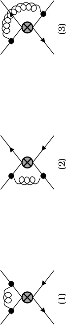
Figure 1: Diagrams contributing to $\langle\hat{Q}_{k}^{\mbox{\tiny bare}}\rangle^{(1)}$.

Now the insertion of $\hat{Q}_{k}$ into the one-loop diagrams of fig. 1 yields a linear combination of the $\hat{Q}_{l}$’s and a new operator with the Dirac structure $Q_{k}^{\prime}=\left[\gamma_{\rho}\gamma_{\sigma}\otimes 1\right]Q_{k}\left[1\otimes\gamma^{\sigma}\gamma^{\rho}\right]$:

$$\langle\hat{Q}_{k}^{\mbox{\tiny bare}}\rangle^{(1)} = d^{(1)}_{kl}\langle\hat{Q}_{l}\rangle^{(0)}+d^{(1)}_{k,Q^{\prime}_{k}}\langle\hat{Q}^{\prime}_{k}\rangle^{(0)}\quad\mbox{no sum on }k,$$ (4)

where $\langle\ldots\rangle^{(0)}$ denote tree level matrix elements. Both coefficients have a term proportional to $1/\varepsilon$ and a finite part. $\hat{Q}_{k}^{\prime}$ is now decomposed into a linear combination of the $\hat{Q}_{l}$’s and an evanescent operator:

$$\hat{Q}_{k}^{\prime\mbox{\tiny bare}} = \left(f_{kl}+a_{kl}\varepsilon\right)\hat{Q}_{l}^{\mbox{\tiny bare}}+\hat{E}_{1}[Q_{k}]^{\mbox{\tiny bare}}+O(\varepsilon^{2}).$$ (5)

Here the $f_{kl}$’s are uniquely determined by the Dirac basis decomposition in $D=4$ dimensions. The $a_{kl}$’s, however, are arbitrary, and a different choice for the $a_{kl}$’s corresponds to a different definition of $\hat{E}_{1}[Q_{k}]=\hat{E}_{1}[Q_{k},\{a_{rs}\}]$. When going beyond the one-loop order new evanescent operators $\hat{E}_{2}[Q_{k}],\hat{E}_{3}[Q_{k}],\ldots$ will appear. Their precise definition is irrelevant for the moment and will be given after (16).

Now in the framework of dimensional regularization the renormalization of some physical operator $\hat{Q}_{k}$ requires counterterms proportional to physical and evanescent operators: We define the renormalization matrix $Z$ by

$$Z_{\psi}^{2}\langle\hat{Q}_{k}^{\mbox{\tiny bare}}\rangle = Z_{kl}\langle\hat{Q}_{l}^{\mbox{\tiny ren}}\rangle+Z_{k,E_{jm}}\langle\hat{E}_{j}[Q_{m}]^{\mbox{\tiny ren}}\rangle\quad.$$ (6)

Here and in the following we will distinguish the renormalization constants related to some evanescent operator $E_{j}[Q_{m}]$ by denoting the corresponding index with $E_{jm}$. (4) and (5) imply that $Z_{kl}^{(1)}$ depends on the $a_{rs}$’s, while $Z_{k,E_{jm}}^{(1)}$ is independent of them. We define the coefficients in the expansion of $Z$ in terms of the gauge coupling constant $g$ and in terms of $\varepsilon$ by

$$Z = 1+\sum_{j}\left(\frac{g^{2}}{16\pi^{2}}\right)^{j}Z^{(j)},\quad\quad Z^{(j)}\,=\,\sum_{k=0}^{j}\frac{1}{\varepsilon^{k}}Z^{(j)}_{k}.$$ (7)

The first analysis of evanescent operators in the context of RG improved QCD corrections to electroweak transitions has been done by Buras and Weisz [5]. They have determined the $a_{kl}$’s by choosing some set of Dirac structures $M=\{\gamma^{(1)}\otimes\tilde{\gamma}^{(1)},\ldots\gamma^{(10)}\otimes\tilde{\gamma}^{(10)}\}$, which forms a basis for $D=4$, and contracting all elements in $M$ with $Q_{k}^{\prime}$ and $Q_{l}$ in (5):

$$\mbox{tr}\left(\gamma^{(m)}q_{k}^{\prime}\tilde{\gamma}^{(m)}\tilde{q}_{k}^{\prime}\right) = (f_{kl}+a_{kl}\varepsilon)\,\mbox{tr}\left(\gamma^{(m)}q_{l}\tilde{\gamma}^{(m)}\tilde{q}_{l}\right)+O(\varepsilon^{2}),$$ (8)

$$\quad\quad\quad\mbox{no sum on }k\mbox{ and on $m$\/=1,\ldots, 10}.$$

The solution of the equations (8) uniquely defines the $f_{kl}+a_{kl}\varepsilon$. In other words, $E_{1}[Q_{k}]$ obeys the equations:

$$E_{1}[Q_{k}]_{ijrs}\gamma^{(m)}_{si}\tilde{\gamma}^{(m)}_{jr} = O(\varepsilon^{2})\quad\quad\quad\mbox{ for $m$\/=1, \ldots,10},$$ (9)

where $i,j,r,s$ are Dirac indices.

Our arguments will not depend on the scheme used for the treatment of $\gamma_{5}$. In the examples we will use a totally anticommuting $\gamma_{5}$. This does not cause any ambiguity in the trace operation in (8), because all Lorentz indices are contracted, so that the traced Dirac string is a linear combination of $\gamma_{5}$ and the unit matrix.

E.g. the choice of

$$M = \{1\otimes 1,1\otimes\gamma_{5},\gamma_{5}\otimes 1,\gamma_{5}\otimes\gamma_{5},\gamma_{\mu}\otimes\gamma^{\mu},\gamma_{\mu}\otimes\gamma^{\mu}\gamma_{5},$$ (10)

$$\quad\gamma_{5}\gamma_{\mu}\otimes\gamma^{\mu},\gamma_{5}\gamma_{\mu}\otimes\gamma^{\mu}\gamma_{5},\sigma_{\mu\nu}\otimes\sigma^{\mu\nu},\gamma_{5}\sigma_{\mu\nu}\otimes\sigma^{\mu\nu}\}$$

gives for $Q$ in (2)

$$Q^{\prime} \!=\! \gamma_{\rho}\gamma_{\sigma}\gamma_{\mu}\left(1-\gamma_{5}\right)\otimes\gamma^{\mu}\gamma^{\sigma}\gamma^{\rho}\left(1-\gamma_{5}\right)=(4-8\varepsilon)Q+E_{1}[Q]+O(\varepsilon^{2})$$ (11)

as in [5]. We remark that this choice $a=-8$ respects the Fierz symmetry, which relates the first to the second diagram in fig. 1.

A basis different from $M$ in (10) yields the same $f_{k,l}$’s, but different $a_{kl}$’s. For example by replacing the sixth and eighth element of $M$ in (10) by $\gamma_{\alpha}\gamma_{\beta}\gamma_{\delta}\otimes\gamma^{\alpha}\gamma^{\beta}\gamma^{\delta}$ and $\gamma_{5}\gamma_{\alpha}\gamma_{\beta}\gamma_{\delta}\otimes\gamma^{\alpha}\gamma^{\beta}\gamma^{\delta}$ one finds

$$Q^{\prime} = 4Q+16\varepsilon(1+\gamma_{5})\otimes(1-\gamma_{5})+E_{1}^{\prime}[Q_{k}]+O(\varepsilon^{2}),$$

instead of (11), i.e.  a different evanescent operator. The Dirac algebra is infinite dimensional for non-integer $D$ and is spanned by $M$ and an infinite set of evanescent Dirac structures. Hence one can reverse the above procedure and first arbitrarily choose the $a_{kl}$’s and then add properly adjusted linear combinations of the evanescent structures to the elements of $M$ such as to obtain the chosen $a_{kl}$’s.

Yet the so defined evanescent operators do not decouple from the physics in four dimensions: In [2, 5] it has been observed that their one-loop matrix elements generally have nonvanishing components proportional to the physical operators $Q_{k}$:

$$\langle\hat{E}_{1}[Q_{k}]^{\mbox{\tiny bare}}\rangle^{(1)} = \left[Z^{(1)}_{0}\right]_{E_{1k},l}\langle\hat{Q}_{l}\rangle^{(0)}+\frac{1}{\varepsilon}\left[Z^{(1)}_{1}\right]_{E_{1k},E_{1k}}\langle\hat{E}_{1}[Q_{k}]\rangle^{(0)}$$ (12)

$$+\frac{1}{\varepsilon}\left[Z^{(1)}_{1}\right]_{E_{1k},E_{2k}}\langle\hat{E}_{2}[Q_{k}]\rangle^{(0)}+O(\varepsilon).$$

Here a second evanescent operator $\hat{E}_{2}$, which will be discussed in a moment, has appeared. Clearly no sum on $k$ is understood in (12) and in following analogous places. In (12) $[Z^{(1)}_{0}]_{E_{1k},l}$ is local, because it originates from the local $1/\varepsilon$–pole of the tensor integrals and a term proportional to $\varepsilon$ stemming from the evanescent Dirac algebra. For the same reason there is no divergence in the term proportional to $\langle\hat{Q}_{l}\rangle^{(0)}$. Now in [2, 5] it has been proposed to renormalize $\hat{E}_{1}$ by a finite amount to cancel this component:

$$\hat{E}_{1}[Q_{k}]^{\mbox{\tiny ren}} = \hat{E}_{1}[Q_{k}]^{\mbox{\tiny bare}}+\frac{g^{2}}{16\pi^{2}}\left\{-\left[Z^{(1)}_{0}\right]_{E_{1k},l}\hat{Q}_{l}\right.$$ (13)

$$\quad\quad-\frac{1}{\varepsilon}\left[Z^{(1)}_{1}\right]_{E_{1k},E_{1k}}\hat{E}_{1}[Q_{k}]$$

$$\quad\quad\left.-\frac{1}{\varepsilon}\left[Z^{(1)}_{1}\right]_{E_{1k},E_{2k}}\hat{E}_{2}[Q_{k}]\right\}+O\left(g^{4}\right).$$

With (13) the renormalized matrix elements of the evanescent operators are $O(\varepsilon)$, so that they do not contribute to the one-loop matching of some Green’s function $G^{\mbox{\tiny ren}}$ in the full renormalizable theory with matrix elements in the effective theory:

$$iG^{\mbox{\tiny ren}} = C_{l}\langle\hat{Q}_{l}\rangle^{\mbox{\tiny ren}}+C_{E_{1k}}\langle\hat{E}_{1}[Q_{k}]\rangle^{\mbox{\tiny ren}}+O\left(g^{4}\right),$$ (14)

i.e. the coefficients $C_{E_{1k}}$ are irrelevant, because they multiply matrix elements which vanish for $D=4$. In [5] it has been further noticed that $Z^{(1)}_{0}$ in (13) influences the two-loop anomalous dimension matrix of the physical operators, so that the presence of evanescent operators indeed has an impact on physical observables. In a different context this has also been observed in [7].

Next we discuss $\hat{E}_{2}[Q_{k}]$, which has entered the scene in (12): When inserting $\hat{E}_{1}[Q_{k}]$ defined in (5) into the one-loop diagrams of fig. 1, one involves

$$Q_{k}^{\prime\prime} = \left[\gamma_{\rho}\gamma_{\sigma}\otimes 1\right]Q_{k}^{\prime}\left[1\otimes\gamma^{\sigma}\gamma^{\rho}\right]$$ (15)

$$= \left[f+a\varepsilon\right]^{2}_{\,kl}Q_{l}+\left(f_{kl}+a_{kl}\varepsilon\right)E_{1}[Q_{l}]$$

$$+\left[\gamma_{\rho}\gamma_{\sigma}\otimes 1\right]E_{1}[Q_{k}]\left[1\otimes\gamma^{\sigma}\gamma^{\rho}\right]$$

$$= \left\{\left[f+a\varepsilon\right]^{2}_{kl}+b_{kl}\varepsilon\right\}Q_{l}+E_{2}[Q_{k}]+O\left(\varepsilon^{2}\right),$$ (16)

which defines $E_{2}[Q_{k}]=E_{2}[Q_{k},\{a_{rs}\},\{b_{rs}\}]$. Only the last term in (15) can contribute to the new coefficients $b_{kl}$. If the projection is performed with e.g. $M$ defined in (10), one finds $b_{kl}=0$ . In our discussion we will keep $b_{kl}$ arbitrary. Clearly, one has a priori to deal with the mixing of an infinite set of evanescent operators $\left\{\hat{E}_{j}[Q_{k}]\right\}$ for each physical operator $\hat{Q}_{k}$, where $\hat{E}_{j+1}[Q_{k}]$ denotes the new evanescent operator appearing first in the one-loop matrix elements of $\hat{E}_{j}[Q_{k}]$.

With the finite renormalization of $\hat{E}_{1}[Q_{k}]$ in (13) the evanescent operators do not affect the physics at the matching scale, at which (14) holds. In order that this will be true at any scale $\mu$, however, one must also ensure that the evanescent operators do not mix into the physical ones. This has been noticed first by Dugan and Grinstein in [6]. For the operator basis $(\vec{Q},\vec{E})=(\hat{Q}_{1},\ldots\hat{Q}_{n},\,\hat{E}_{1}\left[Q_{1}\right],\ldots\hat{E}_{j}\left[Q_{k}\right],\ldots)$ this means that the anomalous dimension matrix

$$\gamma = \left(\begin{array}[]{cc}\gamma_{QQ}&\gamma_{QE}\\ \gamma_{EQ}&\gamma_{EE}\end{array}\right)$$ (19)

has an upper block-triangular form with $\gamma_{EQ}=0$.

The authors of [6] have introduced another way to define the evanescent operators, which is also frequently used: It is easy to see that one can restrict the operator basis $\{Q_{k}\}$ to the set of operators whose Dirac structures $q_{k},\tilde{q}_{k}$ are completely antisymmetric in their Lorentz indices. This is the normal form of Dirac strings introduced in [3]. Dirac strings being antisymmetric in more than four indices vanish in four dimensions and are therefore evanescent. Operators with five antisymmetrized indices correspond to $\hat{E}_{1}$ in our notation, and $\hat{E}_{2}$ would be expressed in terms of a linear combination of Dirac structures with seven and with five antisymmetrized indices. Clearly this method also corresponds to some special choice for the $a_{kl}$’s and $b_{kl}$’s in (5) and (16). Now in [6] the authors have proven that with the use of those definitions and a finite renormalization analogous to (13) the anomalous dimension matrix indeed has the desired block-triangular form, so that the evanescent operators do not mix into the physical ones. While the anomalous dimension matrix is trivially block-triangular at one-loop level, the proof for the two-loop level was given in [6] by the use of the abovementioned special definition of the evanescent operators. The latter, however, has some very special features, which are absent for the general case with arbitrary $a_{kl}$’s and $b_{kl}$’s, e.g. the definition used in [6] automatically yields an anomalous dimension matrix which is tridiagonal in the evanescent sector.

Consider now a definition of the evanescent operators different from the one used in [6]: By inserting the definition (5) of $\hat{E}_{1}\left[Q_{k}\right]$ into (12) one realizes that $\left[Z^{(1)}_{0}\right]_{E_{1k},l}$ depends on the $a_{kl}$’s. Similarly at the two-loop level $\left[Z_{1}^{(2)}\right]_{E_{jk},l}$ depends on the definition (5), so that one has to wonder which choices for the $a_{kl}$’s lead to the desired block-triangular form of $\gamma$ with $\gamma_{EQ}=0$. In the following section we will prove that any choice is permissible. Further we will find that also the $b_{kl}$’s may be chosen completely arbitrary.

On the other hand the physical submatrix $\gamma_{QQ}$ of the anomalous dimension matrix depends on the $a_{kl}$’s as we will show in section 4. Hence the freedom in the definition of the bare evanescent operators induces a renormalization scheme dependence in the physical sector of the operator basis. This feature has not been discussed in the literature so far. As emphasized in the introduction it is of practical importance for NLO calculations to know the scheme transformation formulae for the physical submatrix $\gamma_{QQ}$ and the Wilson coefficients. We will come back to this point in section 4.

3 Block Triangular Anomalous Dimension Matrix

Consider some set of physical operators $\{\hat{Q}_{k}\}$ which closes under renormalization together with the corresponding evanescent operators $\{\hat{E}_{j}[Q_{k}]:j\geq 1\}$. Their $O(\varepsilon)$–parts $a_{rs},b_{rs},\ldots$ are chosen arbitrarily. We want to show that the block of the anomalous dimension matrix describing the mixing of $\hat{E}_{j}[Q_{k}]$ into $\hat{Q}_{l}$ equals zero,

$$\left[\gamma\right]_{E_{jk},l} = 0,$$ (20)

provided one uses the finite renormalization described in (13).

Our sketch will follow the outline of [6], where (20) has been proven by complete induction. At the one-loop level (20) is trivial, and the induction starts in two-loop order: The next-to-leading order contribution to the anomalous dimension matrix $\gamma=\frac{g^{2}}{16\pi^{2}}\gamma^{\left(0\right)}+\left(\frac{g^{2}}{16\pi^{2}}\right)^{2}\gamma^{\left(1\right)}+\ldots$ reads [5]:

$$\gamma^{(1)} = -4Z_{1}^{(2)}-2\beta_{0}Z_{0}^{(1)}+2\left\{Z_{1}^{(1)},Z_{0}^{(1)}\right\}.$$ (21)

The nonzero contributions to (20) in two-loop order are

$$\left[\gamma^{(1)}\right]_{E_{jk},l} = -4\left[Z_{1}^{(2)}\right]_{E_{jk},l}-2\beta_{0}\left[Z_{0}^{(1)}\right]_{E_{jk},l}$$ (22)

$$+2\left\{\left[Z_{1}^{(1)}\right]_{E_{jk},E_{rs}}\left[Z_{0}^{(1)}\right]_{E_{rs},l}+\left[Z_{0}^{(1)}\right]_{E_{jk},m}\left[Z_{1}^{(1)}\right]_{ml}\right\}.$$

Here (22) contains terms which are absent when the special definition of the evanescent operators in [6] is used: In [6] one has $\left[Z^{(1)}\right]_{E_{jk},l}=0$ for $j\geq 2$ contrary to the general case, where any evanescent operator can have counterterms proportional to physical operators.

Next we look at $\left[Z_{1}^{(2)}\right]_{E_{jk},l}$, which stems from the $1/\varepsilon$–term of the $O(g^{4})$–matrix elements of $\hat{E}_{j}[Q_{k}]$. As discussed in [6], these $1/\varepsilon$–terms originate from $1/\varepsilon^{2}$–poles in the tensor integrals multiplying a factor proportional to $\varepsilon$ stemming from the evanescent Dirac algebra. Now in each two-loop diagram the former are related to the corresponding one-loop counterterm diagrams by a factor of 1/2, because the non-local $1/\varepsilon$–poles cancel in their sum [8]. For this to hold it is crucial that the one-loop counterterms are properly adjusted, i.e. that they cancel the $1/\varepsilon$–poles in the one-loop tensor integrals. In the one-loop matrix elements of evanescent operators the latter are multiplied with $\varepsilon$ originating from the Dirac algebra. Hence the proper one-loop renormalization of the evanescent operators must be such as to give matrix elements of order $\varepsilon$, as shown for $E_{1}[Q_{k}]$ in (13).

From the one-loop counterterm graphs one simply reads off:

$$\left[Z_{1}^{(2)}\right]_{E_{jk},l}\!\!\! = \!\!\frac{1}{2}\left\{\left[Z_{0}^{(1)}\right]_{E_{jk},m}\!\left[Z_{1}^{(1)}\right]_{ml}\!\!+\left[Z_{1}^{(1)}\right]_{E_{jk},E_{rs}}\!\left[Z_{0}^{(1)}\right]_{E_{rs},l}\!\!-\beta_{0}\left[Z_{0}^{(1)}\right]_{E_{jk},l}\right\},$$

which yields the desired result when inserted into (22). Here the first two terms stem from insertions of physical and evanescent counterterms to $E_{j}[Q_{k}]$, while the term involving the coefficient of the one-loop $\beta$–function $\beta(g)=-g^{3}/(16\pi^{2})\beta_{0}$ originates from the diagrams with coupling constant counterterms. The terms involving the wave function renormalization constants cancel with those stemming from the factor $Z_{\psi}^{2}$ in (6).

The inductive step in [6] proving (20) to any loop order does not use any special definition of the evanescent and therefore applies unchanged here.

4 Evanescent Scheme Dependences

In this section we will analyze the dependence of the physical part of $\gamma^{(1)}$ given in (21) and of the one-loop Wilson coefficients on $a_{il}$ and $b_{il}$. In practical next-to-leading order calculations one often has to combine Wilson coefficients and anomalous dimension matrices obtained with different definitions of the evanescent operators and it is therefore important to have formulae allowing to switch between them (see e.g. appendix B of [9]).

We start with the investigation of the dependence of $\gamma^{(1)}$ on $a_{il}$. The bare one-loop matrix element

$$\langle\hat{Q}_{k}^{\mbox{\tiny bare}}\rangle^{(1)} = \left\{\frac{1}{\varepsilon}\left[Z_{1}^{(1)}\right]_{kj}+\left[d_{0}^{(1)}\right]_{kj}\right\}\langle\hat{Q}_{j}\rangle^{(0)}+\frac{1}{\varepsilon}\left[Z_{1}^{(1)}\right]_{k,E_{1k}}\langle\hat{E}_{1}[Q_{k}]\rangle^{(0)}$$ (23)

$$+O(\varepsilon)$$

is independent of $a_{il}$, which is evident from (4). $E_{1}[Q_{k}]$ depends linearly on $a_{il}$ through its definition (5) with the coefficient

$$\frac{\partial}{\partial a_{il}}\hat{E}_{1}[Q_{k}] = -\varepsilon\,\delta_{ki}\,\hat{Q}_{l},$$ (24)

so that (23) gives:

$$\frac{\partial}{\partial a_{il}}\left[d_{0}^{(1)}\right]_{kj} = \left[Z_{1}^{(1)}\right]_{k,E_{1k}}\delta_{ki}\delta_{lj},$$ (25)

while $Z_{1}^{(1)}$ is independent of $a_{il}$.

In the same way on can obtain the $a_{kl}$–dependence of $Z_{1}^{(2)}$. (6) reads to two-loop order (cf. (3)):

$$\langle\hat{Q}_{k}^{\mbox{\tiny bare}}\rangle^{(2)} = Z_{kj}^{(2)}\langle\hat{Q}_{j}\rangle^{(0)}+Z_{k,E_{1m}}^{(2)}\langle\hat{E}_{1}[Q_{m}]\rangle^{(0)}+Z_{k,E_{2m}}^{(2)}\langle\hat{E}_{2}[Q_{m}]\rangle^{(0)}$$ (26)

$$+Z_{kr}^{(1)}\langle\hat{Q}_{r}^{\mbox{\tiny ren}}\rangle^{(1)}+Z_{k,E_{1k}}^{(1)}\langle\hat{E}_{1}[Q_{k}]^{\mbox{\tiny ren}}\rangle^{(1)}+\langle\hat{Q}_{k}^{\mbox{\tiny ren}}\rangle^{(2)}.$$

From (16) we know

$$\frac{\partial}{\partial a_{il}}\hat{E}_{2}[Q_{m}] = -\varepsilon\left[f_{mi}\delta_{lj}+\delta_{mi}f_{lj}\right]\hat{Q}_{j},$$ (27)

and from (23) one reads off:

$$\langle\hat{Q}_{r}^{\mbox{\tiny ren}}\rangle^{(1)} = \left[d_{0}^{(1)}\right]_{rj}\langle\hat{Q}_{j}\rangle^{(0)}.$$ (28)

These relations and (25) allow to calculate the derivative of (26) with respect to $a_{il}$. Keeping in mind that the evanescent matrix elements are $O(\varepsilon)$ the $O(1/\varepsilon)$–part of the derivative yields:

$$\frac{\partial}{\partial a_{il}}\left[Z_{1}^{(2)}\right]_{kj} = -\left[Z_{1}^{(1)}\right]_{ki}\left[Z_{1}^{(1)}\right]_{i,E_{1i}}\delta_{lj}+\left[Z_{2}^{(2)}\right]_{k,E_{1i}}\delta_{lj}$$ (29)

$$+\left[Z_{2}^{(2)}\right]_{k,E_{2m}}\left(\delta_{mi}f_{lj}+f_{mi}\delta_{lj}\right),\quad\mbox{no sum on }i.$$

Again $\left[Z_{2}^{(2)}\right]$ can be extracted from the one-loop counterterm diagrams as described in the preceding section:

$$\left[Z_{2}^{(2)}\right]_{k,E_{1i}} = \frac{1}{2}\left[Z_{1}^{(1)}\right]_{ki}\left[Z_{1}^{(1)}\right]_{i,E_{1i}}+\frac{1}{2}\left[Z_{1}^{(1)}\right]_{i,E_{1i}}\left[Z_{1}^{(1)}\right]_{E_{1i},E_{1i}}\delta_{ki}$$

$$-\,\frac{1}{2}\beta_{0}\left[Z_{1}^{(1)}\right]_{i,E_{1i}}\delta_{ki},\quad\quad\mbox{no sum on }i$$

$$\left[Z_{2}^{(2)}\right]_{k,E_{2m}} = \frac{1}{2}\left[Z_{1}^{(1)}\right]_{k,E_{1k}}\left[Z_{1}^{(1)}\right]_{E_{1k},E_{2k}}\delta_{km},\quad\quad\mbox{no sum on }k.$$ (30)

After inserting (30) into (29) we want to substitute the last term in (29). For this we derive both sides of (12) with respect to $a_{il}$ giving:

$$\left[Z_{1}^{(1)}\right]_{E_{1k},E_{2k}}\left(\delta_{ki}f_{lj}+f_{ki}\delta_{lj}\right)\;=$$ (31)

$$\frac{\partial}{\partial a_{il}}\left[Z_{0}^{(1)}\right]_{E_{1k},j}+\left[Z_{1}^{(1)}\right]_{lj}\delta_{ki}-\left[Z_{1}^{(1)}\right]_{E_{1k},E_{1k}}\delta_{ki}\delta_{lj},\quad\mbox{no sum on }k.$$

Finally one has to insert the expression for (29) obtained by the described substitutions into

$$\frac{\partial}{\partial a_{il}}\left[\gamma^{(1)}\right]_{kj} = -4\frac{\partial}{\partial a_{il}}\left[Z_{1}^{(2)}\right]_{kj}+2\left[Z_{1}^{(1)}\right]_{k,E_{1k}}\frac{\partial}{\partial a_{il}}\left[Z_{0}^{(1)}\right]_{E_{1k},j},\quad\mbox{no sum on }k,$$

which follows from (21). The result reads:

$$\frac{\partial}{\partial a_{il}}\left[\gamma^{(1)}\right]_{kj} = -2\left[Z_{1}^{(1)}\right]_{lj}\left[Z_{1}^{(1)}\right]_{i,E_{1i}}\delta_{ki}+2\left[Z_{1}^{(1)}\right]_{ki}\left[Z_{1}^{(1)}\right]_{i,E_{1i}}\delta_{lj}$$ (32)

$$+2\beta_{0}\left[Z_{1}^{(1)}\right]_{i,E_{1i}}\delta_{ki}\delta_{lj},\quad\quad\mbox{no sum on }i.$$

Since the quantities on the right hand side of (32) do not depend on $a_{il}$, one can easily integrate (32) to find the desired relation between two $\gamma$’s corresponding to different choices for $a_{kl}$ in (5). To write the result in matrix form we recall the expression for the physical one-loop anomalous dimension matrix

$$\left[\gamma^{(0)}\right]_{lj} = -2\left[Z_{1}^{(1)}\right]_{lj}$$

and introduce the diagonal matrix $D$ with

$$D_{im} = \left[Z_{1}^{(1)}\right]_{i,E_{1i}}\delta_{im},\quad\quad\quad\mbox{no sum on }i.$$ (33)

Hence

$$\gamma^{(1)}(a^{\prime}) = \gamma^{(1)}(a)+\left[D\cdot(a^{\prime}-a),\gamma^{(0)}\right]+2\,\beta_{0}\,D\cdot(a^{\prime}-a),$$ (34)

where the summation in the row and column indices only runs over the physical submatrices.

(34) exhibits the familiar structure of the scheme dependence of $\gamma^{(1)}$ [10]. Usually scheme dependences are analyzed for a fixed definition of the bare operators and different subtraction procedures. Our situation, however, is more complicated, because we investigate the scheme dependence associated with different definitions of the bare operator basis (i.e. of the bare evanescent operators).

The dependence of the one-loop matrix elements on $a$ can be found easily from (28) and (25):

$$\langle\vec{Q}\rangle^{\mbox{\tiny ren}}(a^{\prime}) = \left[1+\frac{g^{2}}{16\pi^{2}}D\cdot(a^{\prime}-a)\right]\langle\vec{Q}\rangle^{\mbox{\tiny ren}}(a)+O(g^{4}).$$ (35)

Since in (14) $G$ does not depend on $a$ and the evanescent matrix element is $O(\varepsilon)$, the corresponding relation for the Wilson coefficients at the matching scale reads:

$$\vec{C}^{T}(a^{\prime}) = \vec{C}^{T}(a)\left[1-\frac{g^{2}}{16\pi^{2}}D\cdot(a^{\prime}-a)\right]+O(g^{4}).$$ (36)

Hence we can apply the result of [10], which shows that in the renormalization group improved Wilson coefficient the scheme dependences in (34) cancels the one in (35), so that physical observables are scheme independent, provided the hadronic matrix elements are defined scheme independently.

Let us drop some words on the results (34), (35) and (36): In general one would expect scheme transformation formulae involving the full operator basis $(\vec{Q},\vec{E})$. Yet all summations only run over the indices corresponding to the physical operators, the only ingredient from the evanescent sector being the matrix $D$. This is why we could not simply deduce (34) from (35) using the results of [10]. Possible contributions from summations over evanescent operator indices in the matrix products in (34) cannot be inferred from (35), because there they would multiply vanishing matrix elements.

In the same way one can investigate the dependence of $\gamma^{(1)}$ on $b_{il}$ given in (16): While $Z_{1}^{(2)}$ and $Z_{0}^{(1)}$ depend on $b_{il}$, this dependence cancels in (21). Hence neither $\gamma^{(1)}$ nor the one-loop Wilson coefficient are affected by the choice of $b_{il}$.

In general $\gamma^{(0)}$ and $\gamma^{(1)}$ do not commute, so that one has to cope with complicated matrix equations in order to solve the renormalization group equation in next-to-leading order [10]. Now one can use (34) to simplify $\gamma^{(1)}$: By going to the diagonal basis for $\gamma^{(0)}=\mbox{diag}\left(\gamma^{(0)}_{i}\right)$ one can easily find solutions for $a^{\prime}-a$ in (34) which even give $\gamma^{(1)}(a^{\prime})=0$ provided that all $Z_{k,E_{1k}}$’s are nonzero and all eigenvalues of $\gamma^{(0)}$ satisfy $\left|\gamma^{(0)}_{i}-\gamma^{(0)}_{j}\right|\neq 2\beta_{0}$. We will exemplify this in a moment.

A choice for $a_{il}$ which leads to a $\gamma^{(1)}$ commuting with $\gamma^{(0)}$ has been done implicitly in [5]: There the mixing of the two operators $Q_{+}=Q\left({\rm 1}+\tilde{\rm 1}\right)/2$ and $Q_{-}=Q\left({\rm 1}-\tilde{\rm 1}\right)/2$ has been considered, where ${\rm 1}$ and $\tilde{\rm 1}$ denote colour singlet and antisinglet and $Q$ was introduced in (2). Now $Q_{+}$ is self-conjugate under the Fierz transformation, while $Q_{-}$ is anti-self-conjugate, so that $\gamma^{(0)}$ is diagonal to maintain the Fierz symmetry in the leading order renormalization group evolution. As remarked after (11), the definition of $E_{1}[Q]$ in (11) is necessary to ensure the Fierz symmetry in the one-loop matrix elements. Consequently with (11) also $\gamma^{(1)}$ has to obey the Fierz symmetry preventing the mixing of $Q_{+}$ and $Q_{-}$, i.e. yielding a diagonal $\gamma^{(1)}$. A different definition of $E_{1}[Q]$ would result in non-Fierz-symmetric matrix elements, but in renormalization scheme independent expressions they would combine with a non-diagonal $\gamma^{(1)}$ such as to restore Fierz symmetry.

Let us consider the example above to demonstrate that one can pick $a^{\prime}$ such that $\gamma^{(1)}(a^{\prime})=0$: In [5] the definitions

$$E_{1}[Q_{\pm}] = \left(\pm 1-\frac{1}{N}\right)\left[\gamma_{\rho}\gamma_{\sigma}\gamma_{\nu}(1-\gamma_{5})\otimes\gamma^{\nu}\gamma^{\sigma}\gamma^{\rho}(1-\gamma_{5})\right.$$

$$\quad\quad\left.-(4-8\varepsilon)\;\;\gamma_{\nu}(1-\gamma_{5})\otimes\gamma^{\nu}(1-\gamma_{5})\right],$$

i.e. $a_{++}=8(1/N-1),a_{--}=8(1/N+1),a_{+-}=a_{-+}=0$, were adopted yielding a diagonal $\gamma^{(1)}(a)=$diag$\left(\gamma^{(1)}_{+}(a),\gamma^{(1)}_{-}(a)\right)$. From the insertion of $Q_{+}$ and $Q_{-}$ into the diagrams of fig. 1 one finds $Z_{+,E_{1+}}=Z_{-,E_{1-}}=1/4$. Hence if we pick $a^{\prime}_{\pm\pm}=a_{\pm\pm}-2/\gamma^{(1)}_{\pm}(a)/\beta_{0}$ and $a^{\prime}_{\pm\mp}=0$, (34) will imply $\gamma^{(1)}(a^{\prime})=0$.

5 Double Insertions

5.1 Motivation

In the following we will investigate Green functions with two insertions of local operators. Consider first the effective Lagrangian to first order written in terms of bare local operators

$${\cal L}^{\rm I} = C_{k}Z^{-1}_{kl}\hat{Q}^{\mbox{\tiny bare}}_{l}+C_{k}Z^{-1}_{kE_{rl}}\hat{E}_{r}\left[Q_{l}\right]^{\mbox{\tiny bare}}$$ (37)

$$+C_{E_{jk}}Z^{-1}_{E_{jk}l}\hat{Q}^{\mbox{\tiny bare}}_{l}+C_{E_{jk}}Z^{-1}_{E_{jk}E_{rl}}\hat{E}_{r}\left[Q_{l}\right]^{\mbox{\tiny bare}}.$$

According to the procedure presented in the preceding sections, the coefficients $C_{E_{jk}}$ were found to be irrelevant and therefore remained undetermined.

Now consider 4-fermion Green functions with insertion of two local operators from ${\cal L}^{\rm I}$

$$\Bigl{\langle}0\Bigr{|}{\,\rm\bf T\,}\bar{\Psi}_{1}\bar{\Psi}_{2}\left(\frac{i}{2}\int{\rm d}^{D}y{\cal L}^{\rm I}\left(x\right){\cal L}^{\rm I}\left(y\right)\right)\Psi_{3}\Psi_{4}\Bigl{|}0\Bigr{\rangle}.$$ (38)

Such Green functions appear in applications like particle-antiparticle mixing or rare hadron decays. The diagram contributing to lowest order is depicted in fig. 2.

Figure 2: The lowest order diagram contributing to the Green function in (38).

Renormalization of them in general requires additional counterterms proportional to new local dimension-eight operators $\tilde{Q}_{l}$, because the diagram of fig. 2 is divergent:

$${\cal L} = {\cal L}^{\rm I}+{\cal L}^{\rm II}$$ (39)

$${\cal L}^{\rm II} = C_{k}C_{k^{\prime}}\left\{Z^{-1}_{kk^{\prime},l}\tilde{Q}^{\mbox{\tiny bare}}_{l}+Z^{-1}_{kk^{\prime},E_{rl}}\tilde{E}_{r}\left[\tilde{Q}_{l}\right]^{\mbox{\tiny bare}}\right\}$$ (40)

$$+C_{k}C_{E_{j^{\prime}k^{\prime}}}\left\{Z^{-1}_{kE_{j^{\prime}k^{\prime}},l}\tilde{Q}^{\mbox{\tiny bare}}_{l}+Z^{-1}_{kE_{j^{\prime}k^{\prime}},E_{rl}}\tilde{E}_{r}\left[\tilde{Q}_{l}\right]^{\mbox{\tiny bare}}\right\}$$

$$+C_{E_{jk}}C_{E_{j^{\prime}k^{\prime}}}\left\{Z^{-1}_{E_{jk}E_{j^{\prime}k^{\prime}},l}\tilde{Q}^{\mbox{\tiny bare}}_{l}+Z^{-1}_{E_{jk}E_{j^{\prime}k^{\prime}},E_{rl}}\tilde{E}_{r}\left[\tilde{Q}_{l}\right]^{\mbox{\tiny bare}}\right\}$$

$$+\tilde{C}_{k}\tilde{Z}^{-1}_{kl}\tilde{Q}^{\mbox{\tiny bare}}_{l}+\tilde{C}_{k}\tilde{Z}^{-1}_{kE_{rl}}\tilde{E}_{r}\left[\tilde{Q}_{l}\right]^{\mbox{\tiny bare}}$$

$$+\tilde{C}_{E_{jk}}\tilde{Z}^{-1}_{E_{jk}l}\tilde{Q}^{\mbox{\tiny bare}}_{l}+\tilde{C}_{E_{jk}}\tilde{Z}^{-1}_{E_{jk}E_{rl}}\tilde{E}_{r}\left[\tilde{Q}_{l}\right]^{\mbox{\tiny bare}}$$

Here $Z^{-1}_{..,.}\tilde{Q}_{.}$ are the local operator counterterms needed to renormalize the divergences originating purely from the double insertion. Further we have explicitly distinguished physical and evanescent operators. The renormalization constants $Z_{..,.}$, clearly being symmetric in their first two indices, give rise to an inhomogeneity in the RG equation for the Wilson coefficients $\tilde{C}_{k}$, $\tilde{C}_{E_{rs}}$, which we call the anomalous dimension tensor of the double insertion. Note, that this quantity also has three indices, see (57). It has become standard to define the local operator $\tilde{Q}_{l}$ with inverse powers of the coupling constant such that $Z^{-1}_{..,.}=O\left(g^{2}\right)$ to avoid mixing already at the tree level. As an example take $\tilde{Q}=\frac{m^{2}}{g^{2}}\;\gamma_{\mu}\left(1-\gamma_{5}\right)\otimes\gamma^{\mu}\left(1-\gamma_{5}\right)$ for which $\tilde{C}_{l}=O\left(g^{2}\right)$. For simplicity, we assume the $\tilde{Q}_{l}$’s to be linearly independent from the $\hat{Q}_{k}$’s . The $E_{r}\left[\tilde{Q}_{l}\right]$ in (40) are defined analogously to (5) with new coefficients $\tilde{f}_{kl}$, $\tilde{a}_{kl}$, $\tilde{b}_{kl}$, etc. Hence new arbitrary constants $\tilde{a}_{kl}$, $\tilde{b}_{kl}$ potentially causing scheme dependences enter the scene.

Clearly the following questions arise here:

1. Are the coefficient functions $C_{E_{jk}}$ irrelevant also for the double insertions; i.e. do

   $$\left\langle\int{\,\rm\bf T\,}\hat{E}\hat{Q}\right\rangle\hskip 28.45274pt\mbox{and}\hskip 28.45274pt\left\langle\int{\,\rm\bf T\,}\hat{E}\hat{E}\right\rangle$$ (41)

   contribute to the matching procedure and the operator mixing?

2. Does one need a finite renormalization in the evanescent sector of double insertions; if yes, how does this affect the anomalous dimension tensor?

3. How do the $\tilde{C}_{l}$ and anomalous dimension matrices depend on the $a_{kl}$, $b_{kl}$, $\tilde{a}_{kl}$, $\tilde{b}_{kl}$ ?

4. Are the RG improved observables scheme independent?

5.2 Scheme Consistency

In this section we will carry out the program of section 3 for the case of double insertions to answer questions 1 and 2 (on page 1).

Two cases have to be distinguished: The matrix element of the double insertion of the two local renormalized operators can be divergent or finite:

$$\left\langle\frac{i}{2}\int{\,\rm\bf T\,}\hat{Q}_{k}\hat{Q}_{k^{\prime}}\right\rangle = \left\{\begin{array}[]{lcl}\mbox{divergent}&,&\mbox{case 1}\\ \mbox{finite}&,&\mbox{case 2}\end{array}\right..$$ (44)

Case 1 is the generic one, appearing in the calculation of the coefficient $\eta_{3}$ in ${\rm K}^{0}$–$\overline{{\rm K}^{0}}$ mixing [12] or in ${\rm K}\to\pi\nu\bar{\nu}$ [13]. Case 2 appears, if the divergent parts of different contributions to (44) add such that the divergences cancel. It is realized e.g. in the determination of $\eta_{1}$ in ${\rm K}^{0}$–$\overline{{\rm K}^{0}}$ mixing [11]. Therefore we need or do not need a separate renormalization for the double insertion

$$Z^{-1}_{kk^{\prime},l}\left\{\begin{array}[]{clcl}\neq&0&,&\mbox{case 1}\\ =&0&,&\mbox{case 2}\end{array}\right..$$ (47)

Since we need an extra renormalization in case 1, let us introduce the symbol $\left[\frac{i}{2}\int{\,\rm\bf T\,}QQ\right]^{\mbox{\tiny ren}}$ for the completely renormalized operator product constructed from two renormalized local operators $Q$ with an additional renormalization factor for the double insertion.

Let us start the discussion with the matching procedure: At some renormalization scale we have to match Green functions obtained in the full theory with Green functions calculated in the effective theory:

$$-iG^{\mbox{\tiny ren}} = C_{k}C_{k^{\prime}}\left\langle\left[\frac{i}{2}\int{\,\rm\bf T\,}\hat{Q}_{k}\hat{Q}_{k^{\prime}}\right]^{\mbox{\tiny ren}}\right\rangle+C_{k}C_{E_{i^{\prime}k^{\prime}}}\left\langle\left[i\int{\,\rm\bf T\,}\hat{Q}_{k}\hat{E}_{i^{\prime}}\left[Q_{k^{\prime}}\right]\right]^{\mbox{\tiny ren}}\right\rangle$$ (48)

$$+C_{E_{ik}}C_{E_{i^{\prime}k^{\prime}}}\left\langle\left[\frac{i}{2}\int{\,\rm\bf T\,}\hat{E}_{i}\left[Q_{k}\right]\hat{E}_{i^{\prime}}\left[Q_{k^{\prime}}\right]\right]^{\mbox{\tiny ren}}\right\rangle+C_{l}\left\langle\tilde{Q}_{l}\right\rangle$$

$$+\tilde{C}_{E_{jl}}\left\langle\tilde{E}_{j}\left[\tilde{Q}_{l}\right]\right\rangle,$$

where $G^{\mbox{\tiny ren}}$ corresponds e.g. to a “box” function in the full SM. Since the coefficients $C_{E_{jk}}$ must be irrelevant for this matching procedure, one must have

$$Z_{\psi}^{2}\left\langle\left[\frac{i}{2}\int{\,\rm\bf T\,}\hat{E}_{j}\left[Q_{k}\right]\hat{Q}_{k^{\prime}}\right]^{\mbox{\tiny ren}}\right\rangle \stackrel{{\scriptstyle!}}{{=}} \left\{\begin{array}[]{l@{\hspace{1cm}}l}O\left(\varepsilon^{0}\right)\hfil\hskip 28.45274pt&\mbox{in case 1 (LO)}\\ O\left(\varepsilon^{1}\right)\hfil\hskip 28.45274pt&\mbox{in case 1 (NLO and higher)}\\ O\left(\varepsilon^{1}\right)\hfil\hskip 28.45274pt&\mbox{in case 2}\end{array}\right.$$ (52)

and analogously for two insertions of evanescent operators. To understand this recall that the purpose of RG improved perturbation theory is to sum logarithms. In case 1 the LO matching is performed by the comparison of the coefficients of logarithms of the full theory amplitude and the effective theory matrix element (LABEL:CondMatchDouble) (the latter being trivially related to the coefficient of the divergence), while the NLO matching is obtained from the finite part and also involves the matrix elements of the local operators [12, 13]. In case 2 the matching is performed with the finite parts in all orders [11]. In both cases the condition (LABEL:CondMatchDouble) is trivially fulfilled in LO, because the evanescent Dirac algebra gives an additional $\varepsilon$ compared to the case of the insertion of two physical operators. Therefore a finite renormalization for the double insertion turns out to be unnecessary at the LO level. This statement remains valid at the NLO level only in case 2, in case 1 condition (LABEL:CondMatchDouble) no longer holds if one only subtracts the divergent terms in the matrix elements containing a double insertion. With the argumentation preceding (13) one finds that in this case the finite term needed to satisfy the condition (LABEL:CondMatchDouble) is local and therefore can be provided by a finite counterterm.

The operator mixing is more complicated. To deal with this, we need the evolution equation for the Wilson coefficient functions $\tilde{C}_{k}$, $\tilde{C}_{E_{rs}}$, which can be easily derived from the renormalization group invariance of ${\cal L}^{\rm II}$ and reads

$$\mu\frac{{\rm d}}{{\rm d}\mu}\tilde{C}_{l} = \tilde{C}_{l^{\prime}}\tilde{\gamma}_{l^{\prime}l}+C_{k}C_{n}\gamma_{kn,l}$$ (54)

with the anomalous dimension tensor of the double insertion

$$\gamma_{kn,l} = -\left[\gamma_{kk^{\prime}}\delta_{nn^{\prime}}+\delta_{kk^{\prime}}\gamma_{nn^{\prime}}\right]Z^{-1}_{k^{\prime}n^{\prime},l^{\prime}}\tilde{Z}_{l^{\prime}l}-\left[\mu\frac{{\rm d}}{{\rm d}\mu}Z^{-1}_{kn,l^{\prime}}\right]\tilde{Z}_{l^{\prime}l}.$$ (55)

Using the perturbative expansions for the renormalization constants

$$Z^{-1}_{kn,l} = \sum_{j}\left(\frac{g^{2}}{16\pi^{2}}\right)^{j}Z^{-1,\left(j\right)}_{kn,l},\hskip 28.45274ptZ^{-1,\left(j\right)}_{kn,l}=\sum_{i=0}^{j}\frac{1}{\varepsilon^{i}}\left[Z^{-1,\left(j\right)}_{i}\right]_{kn,l}$$ (56)

and $\tilde{Z}$ we derive the perturbative expression for

$$\gamma_{kn,l} = \frac{g^{2}}{16\pi^{2}}\gamma_{kn,l}^{\left(0\right)}+\left(\frac{g^{2}}{16\pi^{2}}\right)^{2}\gamma_{kn,l}^{\left(1\right)}+\ldots$$ (57)

in (55) up to NLO:

$$\gamma^{\left(0\right)}_{kn,l} = 2\left[Z^{-1,\left(1\right)}_{1}\right]_{kn,l}+2\varepsilon\left[Z^{-1,\left(1\right)}_{0}\right]_{kn,l}$$

$$\gamma^{\left(1\right)}_{kn,l} = 4\left[Z^{-1,\left(2\right)}_{1}\right]_{kn,l}+2\beta_{0}\left[Z^{-1,\left(1\right)}_{0}\right]_{kn,l}$$ (58)

$$-2\left[Z^{-1,\left(1\right)}_{0}\right]_{kn,l^{\prime}}\left[\tilde{Z}^{-1,\left(1\right)}_{1}\right]_{l^{\prime}l}-2\left[Z^{-1,\left(1\right)}_{1}\right]_{kn,l^{\prime}}\left[\tilde{Z}^{-1,\left(1\right)}_{0}\right]_{l^{\prime}l}$$

$$-2\left\{\left[Z^{-1,\left(1\right)}_{0}\right]_{kk^{\prime}}\delta_{nn^{\prime}}+\delta_{kk^{\prime}}\left[Z^{-1,\left(1\right)}_{0}\right]_{nn^{\prime}}\right\}\left[Z^{-1,\left(1\right)}_{1}\right]_{k^{\prime}n^{\prime},l}$$

$$-2\left\{\left[Z^{-1,\left(1\right)}_{1}\right]_{kk^{\prime}}\delta_{nn^{\prime}}+\delta_{kk^{\prime}}\left[Z^{-1,\left(1\right)}_{1}\right]_{nn^{\prime}}\right\}\left[Z^{-1,\left(1\right)}_{0}\right]_{k^{\prime}n^{\prime},l}.$$

The indices run over both physical and evanescent operators. The reader may have noticed, that we have used the perturbative expansions of $Z^{-1}$, $\tilde{Z}^{-1}$ rather than $Z$, $\tilde{Z}$ as in the previous sections. This is more convenient for the case of double insertions. Using these equations, the finite renormalization ensuring (LABEL:CondMatchDouble) to hold and the locality of counterterms, one shows in complete analogy to section 3:

$$\gamma^{\left(0\right)}_{E_{rk}l,n} = \gamma^{\left(1\right)}_{E_{rk}l,n}=0\hskip 28.45274pt\mbox{and}\hskip 28.45274pt\gamma^{\left(0\right)}_{E_{rk}E_{sl},n}=\gamma^{\left(1\right)}_{E_{rk}E_{sl},n}=0,$$ (59)

i.e. a double insertion containing at least one evanescent operator does not mix into physical operators. Together with the statement that evanescent operators do not contribute to the matching this proves our method to be consistent at the NLO level. As in the case of single insertions one can pick the $\tilde{a}_{kl}$, $\tilde{b}_{kl}$,…completely arbitrary and then has to perform a finite renormalization for the double insertions containing an evanescent operator in (41). This statement remains valid also in higher orders of the SU(N) interaction, which can be proven analogously to the proof given by Dugan and Grinstein [6] for the case of single insertions.

Now we use the findings above to show the nonvanishing terms in (58) explicitly for the physical submatrix:

$$\gamma^{\left(1\right)}_{kn,l} = 4\left[Z^{-1,\left(2\right)}_{1}\right]_{kn,l}-2\left[Z^{-1,\left(1\right)}_{1}\right]_{kn,E_{1l^{\prime}}}\left[\tilde{Z}^{-1,\left(1\right)}_{0}\right]_{E_{1l^{\prime}}l}$$

$$-2\left[Z^{-1,\left(1\right)}_{1}\right]_{kE_{1k^{\prime}}}\left[Z^{-1,\left(1\right)}_{0}\right]_{E_{1k^{\prime}}n,l}-2\left[Z^{-1,\left(1\right)}_{1}\right]_{nE_{1n^{\prime}}}\left[Z^{-1,\left(1\right)}_{0}\right]_{kE_{1n^{\prime}},l}$$

The last equation encodes the following rule for the correct treatment of evanescent operators in NLO calculations: The correct contribution of evanescent operators to the NLO physical anomalous dimension tensor is obtained by inserting the evanescent one-loop counterterms with a factor of $\frac{1}{2}$ instead of $1$ into the counterterm graphs. Hence the finding of [5] for a single operator insertion generalizes to Green’s functions with double insertions. Here the second term in (LABEL:physdoub) corresponds to the graphs with the insertion of a local evanescent counterterm into the graphs depicted in fig. 1, while the last to terms correspond to the diagrams of fig. 2 with one physical and one evanescent operator.

5.3 Double Insertions: Evanescent Scheme Dependences

In this section we will answer questions 3 and 4 from page 3. Let us first look at the variation of the anomalous dimension tensor $\gamma_{kk^{\prime},l}$ on the coefficients $a_{rs}$. First one notices, that the LO $\gamma^{\left(0\right)}_{kk^{\prime},l}$ is independent of the choice of the $a_{rs}$. In the NLO case one derives in a way completely analogously to the procedure presented in section 4 the following relation

$$\gamma^{\left(1\right)}_{kk^{\prime},l}\left(a^{\prime}\right) = \gamma^{\left(1\right)}_{kk^{\prime},l}\left(a\right)+\left[D\cdot\left(a^{\prime}-a\right)\right]_{ks}\gamma^{\left(0\right)}_{sk^{\prime},l}+\left[D\cdot\left(a^{\prime}-a\right)\right]_{k^{\prime}s}\gamma^{\left(0\right)}_{sk,l}$$ (61)

with the diagonal matrix $D$ from (33). Note that the indices only run over the physical subspace.

The variation of the anomalous dimension tensor $\gamma_{kk^{\prime},l}$ with the coefficients $\tilde{a}_{rs}$ again vanishes in LO, in NLO we find the transformation

$$\gamma^{\left(1\right)}_{kk^{\prime},l}\left(\tilde{a}^{\prime}\right) = \gamma^{\left(1\right)}_{kk^{\prime},l}\left(\tilde{a}\right)+\gamma^{\left(0\right)}_{kk^{\prime},i}\left[\tilde{Z}^{-1,\left(1\right)}_{1}\right]_{iE_{1i}}\left[\tilde{a}^{\prime}-\tilde{a}\right]_{il}-2\beta_{0}\left[Z^{-1,\left(1\right)}_{1}\right]_{kk^{\prime},\tilde{E}_{1i}}\left[\tilde{a}^{\prime}-\tilde{a}\right]_{il}$$ (62)

$$+\left[\gamma^{\left(0\right)}_{kj}\delta_{k^{\prime}j^{\prime}}+\delta_{kj}\gamma^{\left(0\right)}_{k^{\prime}j^{\prime}}\right]\left[Z^{-1,\left(1\right)}_{1}\right]_{jj^{\prime},\tilde{E}_{1i}}\left[\tilde{a}^{\prime}-\tilde{a}\right]_{il}$$

$$-\left[Z^{-1,\left(1\right)}_{1}\right]_{kk^{\prime},\tilde{E}_{1i}}\left[\tilde{a}^{\prime}-\tilde{a}\right]_{is}\tilde{\gamma}^{\left(0\right)}_{sl}$$

As in the case of single insertions, up to the NLO level there exists no dependence of $\gamma$ on the coefficients $b_{rs}$ and also no one on the $\tilde{b}_{rs}$. This provides a nontrivial check of the treatment of evanescent operators in a practical calculation, when the $b_{rs}$, $\tilde{b}_{rs}$ are kept arbitrary: the individual renormalization factors $Z$ each exhibit a dependence on the coefficients $b_{rs}$, $\tilde{b}_{rs}$ but all this dependence cancels, when the $Z$’s get combined to $\gamma$.

Next we will elaborate on the scheme independence of RG improved physical observables. First look at the solution of the inhomogeneous RG equation (54) for the local operator’s Wilson coefficient:

$$\tilde{C}_{l}\!\left(g\left(\mu\right)\right) = \tilde{U}^{\left(0\right)}_{ll^{\prime}}\left(g\!\left(\mu\right),g_{0}\right)\tilde{C}_{l^{\prime}}\!\left(g_{0}\right)$$ (63)

$$+\left[\delta_{ll^{\prime}}+\frac{g^{2}\left(\mu\right)}{16\pi^{2}}\tilde{J}_{ll^{\prime}}\right]\cdot\int\limits_{g_{0}}^{g\left(\mu\right)}{\rm d}g^{\prime}\;\tilde{U}^{\left(0\right)}_{l^{\prime}k}\left(g\!\left(\mu\right),g^{\prime}\right)\left[\delta_{kk^{\prime}}-\frac{g^{\prime 2}}{16\pi^{2}}\tilde{J}_{kk^{\prime}}\right]$$

$$\hskip 28.45274pt\cdot\left[\delta_{nn^{\prime}}+\frac{g^{\prime 2}}{16\pi^{2}}J_{nn^{\prime}}\right]U^{\left(0\right)}_{n^{\prime}t}\left(g^{\prime},g_{0}\right)\left[\delta_{tt^{\prime}}-\frac{g^{\prime 2}}{16\pi^{2}}J_{tt^{\prime}}\right]C_{t^{\prime}}\!\left(g_{0}\right)$$

$$\hskip 28.45274pt\cdot\left[\delta_{mm^{\prime}}+\frac{g^{\prime 2}}{16\pi^{2}}J_{mm^{\prime}}\right]U^{\left(0\right)}_{m^{\prime}v}\left(g^{\prime},g_{0}\right)\left[\delta_{vv^{\prime}}-\frac{g^{\prime 2}}{16\pi^{2}}J_{vv^{\prime}}\right]C_{v^{\prime}}\!\left(g_{0}\right)$$

$$\hskip 28.45274pt\cdot\left\{-\frac{\gamma^{\left(0\right)}_{nm,k^{\prime}}}{\beta_{0}}\frac{1}{g^{\prime}}+\left[\frac{\beta_{1}}{\beta_{0}^{2}}\gamma^{\left(0\right)}_{nm,k^{\prime}}-\frac{\gamma^{\left(1\right)}_{nm,k^{\prime}}}{\beta_{0}}\right]\frac{g^{\prime}}{16\pi^{2}}\right\}.$$

Here the matrices $U^{\left(0\right)}$, $\tilde{U}^{\left(0\right)}$ denote the LO evolution matrices stemming from the solution of the homogeneous RG equations for the Wilson coefficients $C$, $\tilde{C}$, which reads

$$U^{\left(0\right)}\left(g,g_{0}\right) = \left[\frac{g_{0}}{g}\right]^{\frac{{\gamma^{\left(0\right)}}^{T}}{\beta_{0}}}.$$ (64)

We have not labeled the evolution matrices with the renormalization scales $\mu$, $\mu_{0}$ but rather with the corresponding coupling constants $g\left(\mu\right)$ and $g_{0}=g\left(\mu_{0}\right)$. The matrix $J$ is a solution of the matrix equation [10]:

$$J+\left[\frac{{\gamma^{\left(0\right)}}^{T}}{2\beta_{0}},J\right] = -\frac{{\gamma^{\left(1\right)}}^{T}}{2\beta_{0}}+\frac{\beta_{1}}{2\beta_{0}^{2}}{\gamma^{\left(0\right)}}^{T}.$$ (65)

The matrices $\tilde{U}^{\left(0\right)}$, $\tilde{J}$ are defined analogously in terms of $\tilde{\gamma}$. If $\gamma$ transforms according to (34), we know from [10] that $J$ transforms as

$$J(a^{\prime}) = J(a)-\left[D\cdot(a^{\prime}-a)\right]^{T},$$ (66)

which can be easily verified from (35). Hence after inserting (36), (61) and (66) into (63) one finds the independence of $\tilde{C}_{l}$ from the coefficients $a_{kl}$.

In a way similar to the one described above, one treats the scheme dependence coming from the coefficients $\tilde{a}_{kl}$. Here some work has been necessary to prove the cancellation of the scheme dependence connected to $g^{\prime 2}\tilde{J}_{kk^{\prime}}$ and $\gamma^{(1)}_{nm,k^{\prime}}$ in (63): Although it is not possible to perform the integration in (63) without transforming some of the operators to the diagonal basis, one can do the integral for the scheme dependent part of (63), because the part of the integrand depending on $\tilde{a}_{kl}$’s is a total derivative with respect to $g$. There is one important difference compared to the case of the dependence on the $a_{kl}$’s: A scheme dependence of the Wilson coefficient stemming from the lower end of the RG evolution remains. This is a well-known feature of RG improved perturbation theory [10]. This residual $\tilde{a}_{kl}$ dependence must be canceled by a corresponding one in the hadronic matrix element. If the matrix elements are obtained in perturbation theory, one can show that the $\tilde{a}_{kl}$ dependence of the $\tilde{C}_{l}$ gets completely resolved. Finally, as in the case of single insertions [10], one can define a scheme-independent Wilson coefficient for the local operator

$$\overline{\tilde{C}_{l}\!\left(\mu\right)} = \left[\delta_{ll^{\prime}}+\frac{g^{2}\left(\mu\right)}{16\pi^{2}}\cdot\tilde{r}_{l^{\prime}l}\right]\tilde{C}_{l^{\prime}}+\frac{g^{2}\left(\mu\right)}{16\pi^{2}}\cdot\tilde{r}_{nm,l}\cdot C^{\left(0\right)}_{n}\!\left(\mu\right)C^{\left(0\right)}_{m}\!\left(\mu\right)+O\left(g^{4}\right),$$

which multiplies a scheme independent matrix element defined accordingly. It contains the analogue of $\hat{r}$ in [10] for the double insertion

$$\left\langle\frac{i}{2}\int{\,\rm\bf T\,}Q_{n}Q_{m}\right\rangle^{\left(0\right)} = \frac{g^{2}}{16\pi^{2}}\cdot\tilde{r}_{nm,l}\cdot\left\langle\tilde{Q}_{l}\right\rangle^{\left(0\right)}.$$ (68)

6 Inclusive Decays

Inclusive decays are calculated either by calculating the renormalized amplitude and performing a subsequent phase space integration and a summation over final polarizations etc. (referenced as method 1) or by use of the optical theorem, which corresponds to taking the imaginary part of the self-energy diagram depicted in fig. 3 (method 2).

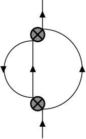
Figure 3: The lowest order self-energy diagram needed for the calculation of inclusive decays via the optical theorem (method 2).

This figure shows that inclusive decays are in fact related to double insertions, but in contrast to the case of section 5 they do not involve local four-quark operators as counterterms for double insertions. In fact, even local two-quark operator counterterms would only be needed to renormalize the real part, but the imaginary part of their matrix elements clearly vanishes. The only scheme dependence to be discussed is therefore the one associated with the $a_{kl}$’s, $b_{kl}$’s, etc., as there are no $\tilde{a}_{kl}$’s $\tilde{b}_{kl}$’s, etc. involved.

To discuss the dependence on the $a_{kl}$’s it is nevertheless advantageous to consider method 1, i.e. the calculation of the amplitude plus the subsequent phase space integration. From section 4 we already know most of the properties of the RG improved amplitude: At the upper renormalization scale the properly renormalized evanescent operators do not contribute and the scheme dependence cancels. Further we know the scheme dependence of the (RG improved) Wilson coefficients at the lower renormalization scale, because with (36) and (34) we can use the result of [10]. What we are left with is the calculation of the properly renormalized operators in perturbation theory, i.e. with on-shell external momenta. Clearly the form of the external states does not affect the scheme dependent terms of the matrix elements, they are again given by (35) and therefore trivially cancel between the Wilson coefficients and the matrix elements, because the scheme dependent terms are independent of the external momenta. Since we now have a finite amplitude which is scheme independent, we may continue the calculation in four dimensions and therefore forget about the evanescent operators. The remaining phase space integration and summation over final polarizations does not introduce any new scheme dependence, therefore we end up with a rate independent of the $a_{kl}$’s, $b_{kl}$’s, etc.

Alternatively one may use the approach via the optical theorem (method 2). Then one has to calculate the imaginary parts of the diagram in fig. 3 plus gluonic corrections. Of course the properly renormalized operators have to be plugged in:

$${\rm Im}\,\left\langle\hat{O}^{\mbox{\tiny ren}}_{k}\hat{O}^{\mbox{\tiny ren}}_{l}\right\rangle$$ (69)

One immediately ends up with a finite rate. What we only have to show is the consistency of the optical theorem with the presence of evanescent operators and with their arbitrary definition proposed in (5), (16). This means that evanescent operators must not contribute to the rate, i.e. diagrams containing an insertion of one or two evanescent operators must be of order $\varepsilon$

$${\rm Im}\,\left\langle\hat{E}_{i}\left[O_{k}\right]^{\mbox{\tiny ren}}\hat{O}^{\mbox{\tiny ren}}_{l}\right\rangle=O\left(\varepsilon\right)\hskip 8.5359pt \hskip 8.5359pt{\rm Im}\,\left\langle\hat{E}_{i}\left[O_{k}\right]^{\mbox{\tiny ren}}\hat{E}_{j}\left[O_{l}\right]^{\mbox{\tiny ren}}\right\rangle=O\left(\varepsilon\right).$$ and (70)

As in the previous sections one can discuss tensor integrals and Dirac algebra separately leading to (70).

7 Conclusions

In this work we have analyzed the effect of different definitions of evanescent operators. We have shown that one may arbitrarily redefine any evanescent operator by $(D-4)$ times any physical operator without affecting the block-triangular form of the anomalous dimension matrix, which ensures that properly renormalized evanescent operators do not mix into physical ones. Especially one is not forced to use the definition of the evanescent operators proposed in [6], whose implementation is quite cumbersome. Then we have analyzed the renormalization scheme dependence associated with the redefinition transformation in the next-to-leading order in renormalization group improved perturbation theory. We stress that it is meaningless to give some anomalous dimension matrix or some Wilson coefficients beyond leading logarithms without specifying the definition of the evanescent operators used during the calculation. In physical observables, however, this renormalization scheme dependence cancels between Wilson coefficients and the anomalous dimension matrix. One may take advantage of this feature by defining the evanescent operators such as to achieve a simple form for the anomalous dimension matrix. Then we have extended the work of [5] and [6] to the case of Green’s functions with two operator insertions and have also analyzed the abovementioned renormalization scheme dependence. For this we have set up the NLO renormalization group formalism for four-quark Green’s functions with two operator insertions, we have derived the renormalization scheme dependence of the corresponding anomalous dimension tensors and defined scheme-independent Wilson coefficients. Finally we have analyzed inclusive decay rates.

References

- [1] G. Bonneau, Nucl. Phys. B167(1980)261, Nucl. Phys. B171(1980)477.
- [2] J. Collins, Renormalization, Cambridge Univ. Press 1984.
- [3] P. Breitenlohner and D. Maison, Comm. Math. Phys. 52(1977)11.
- [4] W. Zimmermann, Ann. Phys. 77(1973)536.
- [5] A. J. Buras and P. H. Weisz, Nucl. Phys. B333(1990)66.
- [6] M. J. Dugan and B. Grinstein, Phys. Lett. B256(1991)239.
-
[7]
M. Bos,
Ann. Phys. 181(1988)177;
C. Schubert, Nucl. Phys. 323(1989)478. - [8] G. ’t Hooft and M. Veltman, Nucl. Phys. B44(1972)189.
- [9] A. J. Buras, M. E. Lautenbacher, M. Misiak, M. Münz, Nucl. Phys. B423(1994)349.
- [10] A. J. Buras, M. Jamin, M. E. Lautenbacher, P. H. Weisz, Nucl. Phys. B370(1992)69.
-
[11]
S. Herrlich and U. Nierste,
Nucl. Phys. B419(1994)292;
S. Herrlich, QCD Korrekturen höherer Ordnung zur – Mischung, in German, PhD Thesis, Technical University of Munich, 1994. -
[12]
S. Herrlich and U. Nierste,
The complete –hamiltonian in the next-to-leading
order, TUM-T31-86/95 (in preparation);
U. Nierste, Indirect CP Violation in the Neutral Kaon System Beyond Leading Logarithms, PhD Thesis, Technical University of Munich, 1995. - [13] G. Buchalla and A. J. Buras, Nucl. Phys. B412(1994)106.