Triply Differential Jet Cross Sections
for Hadron Collisions at Order $\alpha_{s}^{3}$ in QCD

Abstract

We discuss cross sections for $hadron+hadron\to 2\ jets+anything$ in which three jet variables are measured. Such cross sections are useful especially for determining parton distributions. We define a new cross section $d\sigma/dX_{A}\,dX_{B}\,d\eta_{*}$ for which the perturbation theory is nicely behaved even in the kinematic regime where the parton distributions are probed at large momentum fractions. The cross section $d\sigma/dE_{T1}\,d\eta_{1}\,d\eta_{2}$, which has been used in the past, is not so well behaved in this region. We calculate these cross sections at order $\alpha_{s}^{3}$ in QCD.

The experimental investigation of jet production in high energy hadron collisions provides a direct view of the underlying process, parton-parton scattering. It thus provides an opportunity to test quantum chromodynamics (QCD) in some detail. The one jet inclusive cross section $d\sigma/dE_{T}$, where $E_{T}$ is the transverse energy of the jet, provides an excellent probe of any possible breakdown of QCD at short distances [1]. The two jet inclusive cross section $d\sigma/dM_{JJ}$, where $M_{JJ}$ is the invariant mass of the two jet system, plays a similar role, and also tests for possible resonances that might be produced in parton-parton scattering [2]. The two jet angular distribution $[d\sigma/dM_{JJ}\,d\eta_{*}]/[d\sigma/dM_{JJ}]$, where $\eta_{*}$ is half the rapidity difference between the two jets, probes the angular dependence of the Feynman diagrams for parton-parton scattering [3]. These tests have confirmed QCD quite convincingly in a transverse momentum range from 30 GeV all the way to 400 GeV.

It is possible to study inclusive two jet production in even more detail. In a Born level description, the physical process is the scattering of two partons. Each of the two outgoing partons is described by three variables. However, transverse momentum conservation eliminates two of the six total variables, while symmetry about the beam axis makes one variable superfluous. Thus there are three independent variables. So at the Born level one can define, at most, a triply differential cross section for two jet production. For instance, the rapidities $\eta_{1}$ and $\eta_{2}$ of the two partons and the transverse energy $E_{T1}$ of one of them can serve as the three independent variables, leading to a cross section $d\sigma/dE_{T1}\,d\eta_{1}\,d\eta_{2}$. This choice of the three variables, however, is not unique and one may consider other sets of three variables to describe the two outgoing partons and thus other triply differential cross sections. One must also specify how the cross section definition is extended from the case of two partons to the real case of many particles. In this paper we discuss triply differential two-jet cross sections with the goal of using such a cross section to help determine parton distribution functions, particularly at large momentum fractions. We attempt to define the cross section such that the next-to-leading-order contributions are small compared to the Born-level contributions over the entire allowed phase space.

We begin with the cross section $d\sigma/dE_{T1}\,d\eta_{1}\,d\eta_{2}$, which has been measured by both the CDF [4] and D0 [5] groups at Fermilab and calculated at order $\alpha_{s}^{3}$ by Giele, Glover, and Kosower [6]. We define jets according to the standard cone algorithm [7], supplemented by certain algorithms for dealing with overlapping jet cones [1, 8]. Each jet is labeled with variables $E_{T}$, $\eta$ and $\phi$. Here $E_{T}$ is the sum of the absolute values of the transverse momenta of all the particles in the jet cone. (CDF adopts a slightly different definition of $E_{T}$ [1]). The variables $\eta$ and $\phi$ are the $E_{T}$-weighted averages of the rapidities and azimuthal angles of all the particles or calorimeter towers in the jet cone. In each event, we pick the two jets with the highest transverse energies. One of the two jets is defined to be the trigger jet, with transverse energy and rapidity $E_{T1},\,\eta_{1}$. Then $\eta_{2}$ is the rapidity of the other jet. Since there are two ways to choose which jet is the trigger jet, each event contributes to two bins of the cross section.

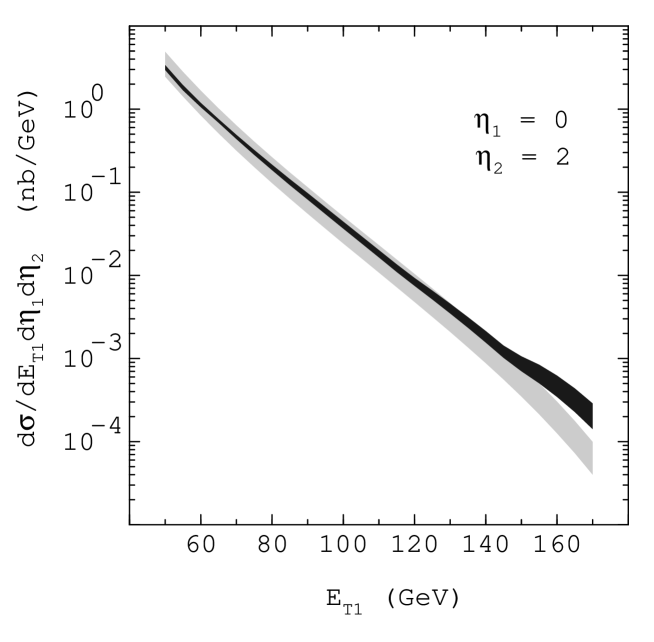
FIG. 1.: The cross section $d\sigma/dE_{T1}\,d\eta_{1}\,d\eta_{2}$ as defined in the text plotted against $E_{T1}$ for $\eta_{1}=0$ and $\eta_{2}=2$. Dark band: full order $\alpha_{s}^{3}$ cross section. Light band: Born cross section (order $\alpha_{s}^{2}$). The bands reflect the variation of the calculated cross section with the renormalization and factorization scales. We use the CTEQ2 parton distributions [9].

The agreement between theory and experiment for $d\sigma/dE_{T1}\,d\eta_{1}\,d\eta_{2}$ is satisfactory, given the experimental and theoretical errors [4, 5, 6]. However, as we shall see, the cross section has large theoretical errors in certain regions of the jet-variable space. In Fig. 1, we show the cross section at $\eta_{1}=0$ and $\eta_{2}=2$ plotted against $E_{T1}$. We plot both the Born cross section and the full order $\alpha_{s}^{3}$ cross section as bands whose widths reflect the theoretical error. The calculated cross section depends on an $\overline{{\rm MS}}$ renormalization scale, $\mu_{UV}$, describing the regulation of ultraviolet divergences, and an $\overline{{\rm MS}}$ factorization scale, $\mu_{CO}$, describing the regulation of collinear divergences. We define these parameters to be $\mu_{UV}=A_{UV}\,E_{T1}/2$, $\mu_{CO}=A_{CO}\,E_{T1}/2$. We choose $(A_{UV},A_{CO})=(1,1)$ as the standard value. Then we determine the bands by calculating the cross sections for $(\log(A_{UV}),\log(A_{CO}))$ chosen at eight points around the circle $\log^{2}(A_{UV})+\log^{2}(A_{CO})=2\log^{2}(2)=0.96$. The upper and lower edges of the error bands correspond to the maximum and minimum, respectively, of the cross section calculated in this range of $(A_{UV},A_{CO})$ values. Such an error band for the order $\alpha_{s}^{N}$ cross section constitutes an estimate of the error induced by omitting order $\alpha_{s}^{N+1}$ and higher contributions to the cross section.

The results shown in Fig. 1 indicate that the theory is well behaved in the central region, $50\ {\rm GeV}<E_{T1}<140\ {\rm GeV}$. However, the theory is not well behaved in the region $140\ {\rm GeV}<E_{T1}$. The $\alpha_{s}^{3}$ corrections to the Born cross section are large and so are the estimated errors. The reason is simple [6]. The allowed kinematic region for the Born cross section for $\eta_{1}=0$ and $\eta_{2}=2$ is $E_{T1}<215\ {\rm GeV}$. Beyond this value of $E_{T1}$, the momentum fraction of the incoming quark from hadron $A$ becomes larger than 1. Although the Born cross section is zero for $E_{T1}>215\ {\rm GeV}$, the full $\alpha_{s}^{3}$ cross section is not, as we will discuss below. Thus for $E_{T1}>215\ {\rm GeV}$, and even for some interval of $E_{T1}$ below this value, the order $\alpha_{s}^{3}$ cross section is effectively a leading order prediction. Generally speaking, leading order cross sections have large estimated errors. This case is no exception. The estimated error is greater than $\pm 15\%$ for $E_{T1}>140\ {\rm GeV}$. At the edge of our plot, the estimated error has reached $\pm 35\%$ and is still growing with $E_{T1}$.

The following general, if somewhat abstract, formalism will allow us to understand how the allowed region at order $\alpha_{s}^{N}$ is related to the definition of the jet cross section. In an order $\alpha_{s}^{N}$ calculation, one can have up to $N$ partons in the final state. These partons can be described by $3N-3$ parameters $v_{i}$ in a space ${\cal V}_{N}$. The definition of a specific triply differential cross section, i.e. of a specific set of three jet-variables, may be understood as a set of maps of the $N$-parton space ${\cal V}_{N}$ into a three dimensional space ${\cal V}_{0}$ of measured jet-variables. Equivalently, we can view the definition as mapping the ${\cal V}_{N}$ into ${\cal V}_{2}$, followed by a map of ${\cal V}_{2}$ into ${\cal V}_{0}$. Thus a point $v$ in ${\cal V}_{N}$ is mapped into a point ${\cal M}_{N}(v)$ in ${\cal V}_{2}$. Now there are many possible sets of maps ${\cal M}$ corresponding to different choices of the three variables. The only restriction comes from the requirement of infrared safety. When, in an $N$-parton configuration, one parton becomes soft or collinear to one of the beams or two partons become collinear, then that configuration must map to the same point in ${\cal V}_{2}$ as the physically equivalent ($N-1$)-parton configuration. This will ensure the cancellation of the relevant singularities in the perturbation theory.

Consider, now, the physically allowed region ${\cal A}_{N}$ in ${\cal V}_{N}$. This is the region determined by $x_{A}<1$ and $x_{B}<1$, where the incoming parton momentum fractions are

$$x_{A}=\sum_{n}{\frac{E_{Tn}}{\sqrt{s}}}\,e^{\eta_{n}},\quad x_{B}=\sum_{n}{\frac{E_{Tn}}{\sqrt{s}}}\,e^{-\eta_{n}}.$$ (1)

This region is mapped into a region ${\cal M}_{N}({\cal A}_{N})$ in ${\cal V}_{2}$ . How does ${\cal M}_{N}({\cal A}_{N})$ compare to ${\cal A}_{2}$? The infrared safety condition implies that

$${\cal M}_{N}({\cal A}_{N})\supseteq{\cal A}_{2}.$$ (2)

To see this, let $\tilde{v}$ be a two parton point in the allowed region ${\cal A}_{2}$. Then consider the physically equivalent point $v$ in ${\cal V}_{N}$ obtained by adding $N-2$ zero momentum partons to $\tilde{v}.$ The infrared safety of the map implies that ${\cal M}_{N}(v)=\tilde{v}$. Since $v\in{\cal A}_{N},$ Eq. (2) follows.

While Eq. (2) holds for any infrared safe definition of a triply differential cross section, the answer to the question of whether ${\cal M}_{N}({\cal A}_{N})$ is equal to ${\cal A}_{2}$ or bigger than ${\cal A}_{2}$ depends on which definition one chooses. Consider the particular cross section $d\sigma/dE_{T1}\,d\eta_{1}\,d\eta_{2}$ defined earlier, and denote the corresponding maps as ${\cal M}_{N}^{{\rm I}}$. It is easy to see that the region ${\cal M}_{N}^{{\rm I}}({\cal A}_{N})$ is bigger than ${\cal A}_{2}$. For instance, the three parton final state with

$$E_{T1} = 220\ {\rm GeV},\ \eta_{1}=0,\ \phi_{1}=0,$$ (3)

$$E_{T2} = 120\ {\rm GeV},\ \eta_{2}=2,\ \phi_{2}=\pi,$$ (4)

$$E_{T3} = 100\ {\rm GeV},\ \eta_{3}=0,\ \phi_{3}=\pi$$ (5)

has $x_{A}=0.67$, $x_{B}=0.19$. This kinematically allowed state is mapped to the two parton final state with

$$E_{T1} = 220\ {\rm GeV},\ \eta_{1}=0,\ \phi_{1}=0,$$ (6)

$$E_{T2} = 220\ {\rm GeV},\ \eta_{2}=2,\ \phi_{2}=\pi.$$ (7)

This state has $x_{B}=0.14$ but $x_{A}=1.03$, so it is not in the kinematically allowed region ${\cal A}_{2}$ and ${\cal M}_{N}^{{\rm I}}({\cal A}_{N})\supset{\cal A}_{2}$.

The results depicted in Fig. 1 suggest that the cross section $d\sigma/dE_{T1}\,d\eta_{1}\,d\eta_{2}$ provides a useful tool for exploring QCD and testing parton distributions, but that there are difficulties resulting from the fact that the allowed regions ${\cal M}_{N}({\cal A}_{N})$ at order $\alpha_{s}^{N}$ are larger than ${\cal A}_{2}$, the region allowed at the Born level. Now the question arises, can we define a triply differential jet cross section such that the maps of all of the allowed regions ${\cal M}_{N}({\cal A}_{N})$ equal ${\cal A}_{2}$? In this case the perturbative result can be well behaved over the entire allowed region. The answer is that there are many such solutions and one particular choice stands out as being particularly simple.

We define a cross section $d\sigma/dX_{A}\,dX_{B}\,d\eta_{*}$ as follows. Define jets according to the standard cone algorithm [7]. In each event, pick the two jets with the highest transverse energies $E_{T}$. Let

$$\eta_{*}=|\eta_{1}-\eta_{2}|/2,$$ (8)

where $\eta_{1}$ and $\eta_{2}$ are the rapidities of these two leading jets. (That is, $\eta$ is the $E_{T}$-weighted average of the rapidities of all the particles or calorimeter towers in the jet cone [7].) Let

$$X_{A}=\sum_{i\in{\rm jets}}{\frac{E_{Ti}}{\sqrt{s}}}\ e^{\eta_{i}},\quad X_{B}=\sum_{i\in{\rm jets}}{\frac{E_{Ti}}{\sqrt{s}}}\ e^{-\eta_{i}}.$$ (9)

The sum here runs over all of the particles (or calorimeter towers) in either of the jet cones.

Let us call the maps corresponding to this definition ${\cal M}_{N}^{{\rm II}}$. It is easy to see that the allowed regions ${\cal M}_{N}^{{\rm II}}({\cal A}_{N})$ are all the same. For an allowed $N$-parton configuration, the true momentum fractions $x_{A}$ and $x_{B}$, as given in Eq. (1), are less than 1. From Eq. (9) we obtain

$$X_{A}\leq x_{A},\quad X_{B}\leq x_{B}.$$ (10)

Thus an allowed $N$-parton state must have $X_{A}<1$ and $X_{B}<1$. In the two parton final state with the same jet variables, the momentum fractions of the final state partons are precisely $X_{A}$ and $X_{B}$. Thus an allowed $N$-parton final state is mapped into an allowed two-parton final state. That is, ${\cal M}_{N}^{{\rm II}}({\cal A}_{N})\subseteq{\cal A}_{2}$. Since we already know from Eq. (2) that ${\cal M}_{N}^{{\rm II}}({\cal A}_{N})\supseteq{\cal A}_{2}$, we have

$${\cal M}_{N}^{{\rm II}}({\cal A}_{N})={\cal A}_{2}.$$ (11)

The numerical example used earlier illustrates the point. We considered the allowed three parton configuration with parameters $v$ given by Eq. (4). With the new definition, this state has jet variables $X_{A}=0.61$, $X_{B}=0.13$, $\eta_{*}=1$. The corresponding two parton state $\tilde{v}={\cal M}_{3}^{{\rm II}}(v)$ is

$$E_{T1} = 166\ {\rm GeV},\ \eta_{1}=-0.23,\ \phi_{1}=0,$$ (12)

$$E_{T2} = 166\ {\rm GeV},\ \eta_{2}=1.77,\ \ \ \,\phi_{2}=\pi$$ (13)

with $x_{A}=X_{A}=0.61$ and $x_{B}=X_{B}=0.13$. Thus with the new definition the two parton state is kinematically allowed.

The variables $X_{A}$ and $X_{B}$ are conceptually straightforward. To calculate $X_{A}$, for instance, we sum of the plus-components $k_{i}^{+}=(k_{i}^{0}+k_{i}^{3})/\sqrt{2}$ of the four-momenta of the particles inside both jet cones and divide by the plus-component of hadron $A$’s momentum. On the experimental side, we note that, for large rapidity $\eta_{i}$, $E_{Ti}\exp(\eta_{i})$ is approximately twice the energy of particle $i$. Since calorimeters directly measure energy, the spreading of a large rapidity jet over a region of rapidity in the detector should not much affect the measurement of $X_{A}$.

The cross section $d\sigma/dX_{A}\,dX_{B}\,d\eta_{*}$ takes a very simple form at the Born level:

$$X_{A}^{2}X_{B}^{2}s\ \frac{\,d\sigma}{dX_{A}\,dX_{B}\,d\eta_{*}}=$$ (15)

$$\sum_{a,b}X_{A}f_{a/A}(X_{A},\mu_{A})\,X_{B}f_{b/B}(X_{B},\mu_{B})\,\alpha_{s}^{2}(\mu_{UV})\,H_{ab}(\eta_{*}).$$

Here $f_{a/A}(X_{A},\mu_{A})$ is the parton distribution function for finding a parton of type $a$ in hadron $A$, evaluated at some scale $\mu_{A}$; $f_{b/B}(X_{B},\mu_{B})$ is the corresponding function for hadron $B$. There are two powers of $\alpha_{s}$ evaluated at a scale $\mu_{UV}$. Finally there is a function $H_{ab}(\eta_{*})$ that gives the angular distribution for 2 parton $\to$ 2 parton scattering at c.m. energy squared $\hat{s}$:

$${\frac{d\sigma(a+b\to a^{\prime}+b^{\prime})}{d\eta_{*}}}={\frac{\alpha_{s}^{2}}{\hat{s}}}\ H_{ab}(\eta_{*}).$$ (16)

The incoming partons are of type $a,b$ here and we sum over types of outgoing partons. We see that the variables $X_{A}$, $X_{B}$, and $\eta_{*}$ are well adapted to probing the factors in the Born-level cross section, especially the parton distribution functions.

What of the scales $\mu$? Some sensible choices are suggested by the kinematics of parton-parton scattering at the Born level, as seen in the parton-parton c.m. frame. One choice might be half the energy of each of the outgoing partons, $E/2=[X_{A}X_{B}s]^{1/2}/4$, while another might be half the transverse momentum of each of the outgoing partons, $P_{T}/2=[X_{A}X_{B}s]^{1/2}/[4\cosh(\eta_{*})]$. In our next-to-leading order calculation, we use a compromise between these two approaches:

$$\mu_{UV} = A_{UV}{\ \sqrt{X_{A}X_{B}s}/[4\cosh(0.7\eta_{*})]},$$ (17)

$$\mu_{A} = A_{CO}{\ \sqrt{X_{A}X_{B}s}/[4\cosh([1-X_{A}]\eta_{*})]},$$ (18)

$$\mu_{B} = A_{CO}{\ \sqrt{X_{A}X_{B}s}/[4\cosh([1-X_{B}]\eta_{*})]}.$$ (19)

Here the factors $A_{UV}$ and $A_{CO}$ are adjustable. Any choices of these $A$’s that are of order 1 would be reasonable.

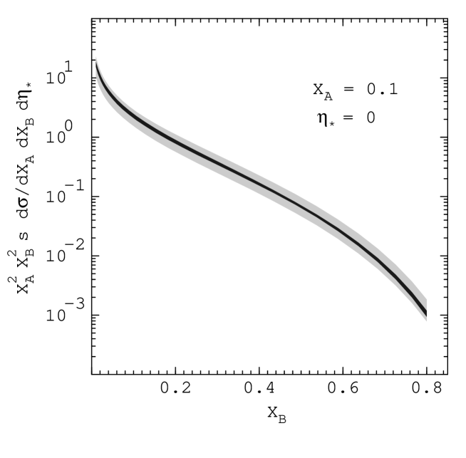
FIG. 2.: The cross section $d\sigma/dX_{A}\,dX_{B}\,d\eta_{*}$ as defined in the text plotted against $X_{B}$ for $X_{A}=0.1$ and $\eta_{*}=0$. Dark band: full order $\alpha_{s}^{3}$ cross section. Light band: Born cross section (order $\alpha_{s}^{2}$). The bands reflect the variation of the calculated cross section with the renormalization and factorization scales. We use the CTEQ2 parton distributions [9].

In Fig. 2, we show the cross section $d\sigma/dX_{A}\,dX_{B}\,d\eta_{*}$ at $X_{A}=0.1$ and $\eta_{*}=0$ plotted against $X_{B}$. We plot both the Born cross section and the full order $\alpha_{s}^{3}$ cross section, in each case as a band whose width reflects the theoretical error as determined by choosing $(\log(A_{UV}),\log(A_{CO}))$ at eight points around the circle $\log^{2}(A_{UV})+\log^{2}(A_{CO})=2\log^{2}(2)=0.96$, just as in Fig. 1.

The results shown in Fig. 2 indicate that the theory is well behaved in the entire $X_{B}$ range shown, even out to quite large $X_{B}$. The $\alpha_{s}^{3}$ corrections are not large and the $\alpha_{s}^{3}$ calculation has small estimated errors from higher order contributions, about 10%.

Our calculations in this paper are based on the subtraction algorithm and corresponding computer code for calculating next-to-leading order jet cross sections described in Ref. [10]. The desired definitions of jets and jet variables are inserted into certain small subroutines in the code. A new feature compared to previous versions of the code is that the program directly calculates the so-called $K$-factor, the ratio of the full order $\alpha_{s}^{3}$ cross section to the Born cross section. This has technical advantages stemming from the fact that the $K$-factor is normally nearly constant as a function of the three jet variables, at least for an appropriately defined cross section as here.

We conclude with a caveat. We have seen that the cross section $d\sigma/dX_{A}\,dX_{B}\,d\eta_{*}$ is reasonably well behaved for small $1-X_{A}$ or $1-X_{B}$. Nevertheless, the example of the Drell-Yan cross section teaches us that the perturbation series will contain terms with factors of $\log(1-X_{A})$ and $\log(1-X_{B})$. A summation of these logarithmic terms will be useful, and perhaps necessary, in order to explore with precision the small $1-X_{A}$ and $1-X_{B}$ regions. Substantial progress along these lines has been made in the Drell-Yan case [11].

This work was supported by the United States Department of Energy. We thank E. Kovacs, S. Kuhlmann, H. Weerts and Z. Kunszt for helpful conversations. We thank W. Giele for help in comparing our results to those of Ref. [6].

REFERENCES

- [1] S. D. Ellis, Z. Kunszt and D. E. Soper, Phys. Rev. Lett. 62, 726 (1988); Phys. Rev. Lett. 64, 2121 (1990); F. Aversa, M. Greco, P. Chiappetta and J. P. Guillet, Phys. Lett. 210B, 225 (1988); Phys. Lett. B 211, 465 (1988); Nucl. Phys. B327, 105 (1989) Z. Phys. C46, 253 (1990); Phys. Rev. Lett. 65, 401 (1990); CDF Collaboration, F. Abe et al., Phys. Rev. Lett. 68, 1104 (1992); Phys. Rev. Lett. 70, 1376 (1993); Phys. Rev. D 45, 1448 (1992).
- [2] CDF Collaboration, F. Abe et al., Phys. Rev. D 41, 1722 (1990).
- [3] S. D. Ellis, Z. Kunszt and D. E. Soper, Phys. Rev. Lett. 69, 1496 (1992);
- [4] CDF Collaboration, F. Abe et al., Fermilab Report No. FERMILAB-Conf-93/201-E (1993).
- [5] D0 Collaboration, F. Nang et al., Fermilab Report No. FERMILAB-Conf-94/323-E (1994).
- [6] W. T. Giele, E. W. N. Glover, and D. A. Kosower, Phys. Rev. Lett. 73, 2019 (1994); Fermilab Preprint FERMILAB-Pub-94/382-T, Bulletin Board: hep-ph@xxx.lanl.gov - 9412338.
- [7] J. E. Huth, N. Wainer, K. Meier, N. Hadley, F. Aversa, M. Greco, P. Chiappetta, J. Ph. Guillet, S. D. Ellis, Z. Kunszt and D. E. Soper, Proc. Summer Study on High Energy Physics, Research Directions for the Decade, Snowmass, CO, Jun 25 - Jul 13, 1990.
- [8] S. D. Ellis and D. E. Soper, Phys. Rev. D 48, 3160 (1993).
- [9] H. L. Lai, J. Botts, J. Huston, J. G. Morfin, J. F. Owens, J.-W. Qiu, W.-K. Tung and H. Weerts, Michigan State Preprint MSU-HEP-41024 (1994), Bulletin Board: hep-ph@xxx.lanl.gov - 9410404.
- [10] S. D. Ellis, Z. Kunszt and D. E. Soper, Phys. Rev. D 40, 2188 (1989); Z. Kunszt and D. E. Soper, Phys. Rev. D 46, 192 (1992).
- [11] J.-W. Qiu and G. Sterman, Nucl. Phys. B353, 105 (1991); Nucl. Phys. B353, 137 (1991); H. Contopanagos and G. Sterman, Nucl. Phys. B400, 211 (1993); Nucl. Phys. B419, 77 (1994).