CONSTRUCTING ${\cal CP}$-ODD OBSERVABLES

Abstract

In these lectures we review the general features necessary to construct ${\cal CP}$ odd observables and study illustrative examples. We present in some detail the case of ${\cal CP}$ violation in hyperon decays. We survey different observables sensitive to ${\cal CP}$ violating new physics, concentrating on the search for electric-dipole moments in high energy experiments.

1 Discrete Symmetries

We start by recalling some basic properties of the discrete symmetries corresponding to parity, charge conjugation and time reversal invariance. The first two are implemented by unitary transformations, and the last one by an anti-unitary transformation in free field theories.[1, 2, 3]

Parity $({\cal P})$ is the discrete symmetry that takes $\vec{x}\leftrightarrow-\vec{x}$. For free, single particle, momentum eigenstates, this simply reverses the particle momentum up to a phase $\eta=\pm 1$:

$${\cal P}\ket{\Psi(\vec{k},\vec{s})}=\eta^{\cal P}\ket{\Psi(-\vec{k},\vec{s})}.$$ (1)

For scalars the intrinsic phase is the same for particle and anti-particle, whereas for fermions it is opposite. Photons have intrinsic parity $\eta=-1$. For angular momentum eigenstates, a phase of $(-)^{l}$ is introduced by the parity transformation.

Charge conjugation $({\cal C})$ is the discrete symmetry that transforms particles into antiparticles up to a phase. For both scalars and fermions the intrinsic phase associated with an anti-particle is the complex conjugate of the intrinsic phase associated with the corresponding particle. The intrinsic phase for photons is $\eta=-1$. The phase associated with each particle is convention dependent and unphysical.

The discrete symmetry corresponding to a successive application of $({\cal P})$ and $({\cal C})$, $({\cal CP})$, is the subject of these lectures. Some examples of a ${\cal CP}$ transformation on common single particle states within our phase convention are:

$${\cal CP}\ket{\pi^{0}} = -\ket{\pi^{0}}$$

$${\cal CP}\ket{\pi^{\pm}} = -\ket{\pi^{\mp}}$$

$${\cal CP}\ket{K^{0}} = -\ket{\bar{K}^{0}}.$$ (2)

An important system is that of a fermion anti-fermion pair in their center of mass frame. This system transforms under ${\cal CP}$ as:

$${\cal CP}\ket{e^{-}(\vec{k},\vec{s})e^{+}(-\vec{k},\vec{s}^{\prime})} = {\cal C}(-)\ket{e^{-}(-\vec{k},\vec{s})e^{+}(\vec{k},\vec{s}^{\prime})}$$ (3)

$$= (-)\ket{e^{+}(-\vec{k},\vec{s})e^{-}(\vec{k},\vec{s}^{\prime})}$$

$$= \ket{e^{-}(\vec{k},\vec{s}^{\prime})e^{+}(-\vec{k},\vec{s})}$$

the net effect of the ${\cal CP}$ transformation is to interchange the spin vectors of particle and anti-particle. This result implies that it is possible to construct simple ${\cal CP}$-odd observables for processes that occur in $e^{+}e^{-}$ or $p\overline{p}$ colliders when the spin density matrix for the initial state is symmetric under a spin interchange.[4, 5] We will use this transformation repeatedly in the construction of ${\cal CP}$ odd observables.

Time reversal invariance $({\cal T})$ is the symmetry that takes $t\leftrightarrow-t$ classically. The requirement that under this transformation a Hamiltonian does not change sign, leads to the anti-unitary nature of ${\cal T}$.[3] For free, single particle, momentum eigenstates, the effect of this transformation is to reverse the direction of both momentum and spin vectors. There is also an intrinsic phase associated with this transformation. It is the same for particle and anti-particle. The anti-unitary nature of the transformation is responsible for the additional effect of interchanging incoming states into outgoing states and viceversa:

$${\cal T}\ket{p(\vec{k},\vec{s})}=\bra{p(-\vec{k},-\vec{s})}\equiv\bra{\tilde{p}}.$$ (4)

We will use the symbol $\tilde{p}$ to denote a reversal of all momenta and spin vectors in the state $p$.

The anti-unitary nature of the time reversal operator is also important when applying this transformation to multi-particle states. If the multi-particle state is a direct product of free (non-interacting, asymptotic) momentum eigenstates, then the ${\cal T}$ transformation is a straightforward generalization of Eq. 4. For angular momentum eigenstates, the transformation is:

$${\cal T}\ket{j,m}=(-)^{j+m}\ket{j,-m}.$$ (5)

However, if the multi-particle state consists of interacting particles, the interchange of “in” and “out” states plays a crucial role, as we will see in the example of hyperon decay. In general, the transformation is:

$${\cal T}\ket{f_{out}}=\bra{\tilde{f}_{in}}=\bra{\tilde{f}_{out}}S^{\dagger}.$$ (6)

The action of the anti-unitary operator ${\cal T}$ can be expressed in terms of that of a unitary operator $U_{T}$ following Wigner:[1, 6]

$${\cal T}\ket{n} = U_{T}\ket{n}^{*}$$

$${\cal T}{\cal O}{\cal T}^{-1} = U_{T}{\cal O}^{*}U_{T}^{\dagger}.$$ (7)

It is convenient to define an operator $(T)$ sometimes called “naive”-time reversal transformation. This operator which is not the same as the time reversal operator ${\cal T}$, simply reverses the sign of all momentum and spin vectors: $T\ket{p}=\ket{\tilde{p}}$. $T$ is a useful operator to classify ${\cal CP}$ odd observables.

Throughout these lectures we will assume that the combined operation of parity, charge conjugation and time reversal, ${\cal CP}{\cal T}$, is a good symmetry of the theories under consideration. As is well known from the ${\cal CP}{\cal T}$ theorem, this will be true for any theory defined by a hermitian, Lorentz invariant, normal ordered product of fields quantized with the usual spin-statistics connection.[2] Because of this assumption, ${\cal CP}$ violation (denoted by $\not\!\!{\cal CP}$) will be equivalent to ${\cal T}$ violation ($\not\!{\cal T}$).

2 Ingredients for $\not\!\!{\cal CP}$ Observables

A ${\cal CP}$-odd observable is an observable whose expectation value vanishes if ${\cal CP}$ is conserved. There are several ingredients necessary to construct ${\cal CP}$-odd observables.

The first of these ingredients is to have a ${\cal CP}$ violating phase in the theory. The theory must have a non-trivial phase (one that cannot be removed by field redefinitions) in order to violate ${\cal CP}$. As you already saw in lectures by previous speakers, the minimal standard model with three generations has one such phase.[7] This phase appears in the CKM matrix, and in the original parameterization of Kobayashi and Maskawa it is called $\delta$.[8]

Once we have a theory that contains a ${\cal CP}$ violating phase, we must still construct an observable that depends on the value of that phase. One possibility is to identify a process that is forbidden by ${\cal CP}$ invariance, typically a transition between ${\cal CP}$ eigenstates with different ${\cal CP}$ eigenvalues. Most processes, however, involve states that are not ${\cal CP}$ eigenstates. In this case ${\cal CP}$ invariance predicts relations between the process and its ${\cal CP}$ conjugate process. One can then construct observables that test these predictions.

A $\not\!\!{\cal CP}$ observable that compares a pair of ${\cal CP}$ conjugate processes, will vanish unless there are several amplitudes contributing to the processes, and these amplitudes can interfere. This can be seen by considering the process $i\rightarrow f$ and assuming that there is only one amplitude contributing to it, so that $M(i\rightarrow f)=e^{i\phi}A_{1}$. Even if this amplitude contains the ${\cal CP}$ violating phase $\phi$, observables will be proportional to $|M|^{2}=A_{1}^{2}$ and thus independent of $\phi$. However, if there is at least one other amplitude (with a different phase), then $M(i\rightarrow f)=e^{i\phi}A_{1}+A_{2}$, and observables will be proportional to $|M|^{2}=(A_{1}\cos\phi+A_{2})^{2}+A_{1}^{2}\sin^{2}\phi$. Interference is, therefore, necessary for observables to depend on ${\cal CP}$ violating phases. However, we do not yet have ${\cal CP}$-odd observables, since $|M|^{2}$ above does not vanish as $\phi\rightarrow 0$. It is still possible to extract information on ${\cal CP}$ violation from precision measurements of these observables. A known example is the determination of the CKM parameters by measurements of the sides of the unitarity triangle.[9]

The construction of ${\cal CP}$-odd observables (that vanish when $\phi\rightarrow 0$) requires an additional (usually ${\cal CP}$-conserving) phase. A very simple way to see this, is to rewrite the previous amplitude for our process $i\rightarrow f$ as $M(i\rightarrow f)=A_{1}\cos\phi+A_{2}+iA_{1}\sin\phi$. One can then see immediately, that it is only possible to obtain a term linear in $\sin\phi$ in the matrix element squared $|M|^{2}$, if there is another imaginary term in $M$ to interfere with the $iA_{1}\sin\phi$ term. If, for example, there is another ${\cal CP}$ conserving amplitude $A_{3}e^{i\delta}$ contributing to our process $i\rightarrow f$, it will be possible to find observables proportional to $\sin\phi\sin\delta$. A ${\cal CP}$ conserving phase such as this, usually arises from final state interactions (from the existence of real intermediate states beyond the Born approximation). You have already seen an example of this type of phase in the study of ${\cal CP}$ violation in the $K^{0}\rightarrow\pi\pi$ system[7]. In that case you wrote, for example, $A(K^{0}\rightarrow\pi^{+}\pi^{-})=A_{0}e^{i\delta_{0}}+A_{2}/\sqrt{2}e^{i\delta_{2}}$. In this expression, any ${\cal CP}$ violating phases are included in $A_{0},A_{2}$, and the phases $\delta_{0}$, $\delta_{2}$ are the $\pi\pi$ scattering phase shifts in the $I=0$, $I=2$ channels.

Using the discrete symmetry $T$ (recall that this is not the same as time reversal invariance) to classify ${\cal CP}$-odd observables, one finds in general that ${\cal CP}$-odd and $T$-even observables are proportional to quantities like $\sin\delta\sin\phi$. That is, that the simultaneous presence of a ${\cal CP}$ violating phase and a ${\cal CP}$ conserving “unitarity” phase is needed in order for the observable not to vanish. On the other hand, $T$-odd observables are found to be proportional to quantities like $\sin\delta\cos\phi+\sin\phi\cos\delta$. This result is consistent with the statement that $T$ violation is not the same as ${\cal CP}$ violation. Using $T$-odd quantities it is possible to construct ${\cal CP}$-odd observables that do not require additional “unitarity” phases.

We will see how this works in more detail when we discuss specific examples later on. At this point, however, it is convenient to ask two questions.

• In view of our earlier discussion, how is it possible to get $T$-odd and ${\cal CP}$-odd observables that do not require a “unitarity” phase? A typical $T$-odd quantity contains the triple product of three vectors (recall that $T$ reverses the sign of momentum and spin vectors), like $\vec{p_{1}}\cdot\vec{p_{2}}\times\vec{p_{3}}$. Such a quantity must come from a Lorentz invariant expression of the form $\epsilon^{\mu\nu\alpha\beta}k_{\mu}p_{1\nu}p_{2\alpha}p_{3\beta}$ (for example in the rest frame of $k$). In the case of amplitudes involving fermions, we would obtain an expression like this one from the Dirac trace of four $\gamma$ matrices and a $\gamma_{5}$, which has a factor of $i$ relative to expressions without the epsilon tensor. This relative phase is the one taking the place of the “unitarity” phase needed for a ${\cal CP}$-odd observable.

• Why is it possible to obtain a $T$-odd observable that does not violate ${\cal CP}$? As we said before, this is simply because $T$ is not the same as time reversal invariance. In some detail, we can see the origin of such $T$-odd observables when we go beyond the Born approximation for a given process. Writing the $S$-matrix as $S=I-iM$, unitarity implies that

  $$S^{\dagger}S=I = (I+iM^{\dagger})(I-iM)$$

  $$= I-i(M-M^{\dagger})+M^{\dagger}M$$

  $$\Rightarrow\;\;i(M-M^{\dagger}) = M^{\dagger}M.$$ (8)

  Taking the matrix element of this last expression between states $f$ and $i$, with the definition $M_{if}\equiv\bra{f}M\ket{i}$, and noticing that $\bra{f}M^{\dagger}\ket{i}=\bra{i}M\ket{f}^{*}$ one finds:

  $$i(M_{if}-M^{*}_{fi})=\sum_{n}M^{*}_{fn}M_{in}.$$ (9)

  This shows that for the left hand side to be different from zero, there must exist real intermediate states, $n$, that couple to $i$ and $f$. This is shown schematically in Figure 1.

  

  Figure 1: Unitarity phases from real intermediate states.

  Assuming time reversal invariance (and hence ${\cal CP}$ invariance) it is possible to relate the matrix elements for the process $i\rightarrow f$ and for its $T$ conjugated process $\tilde{i}\rightarrow\tilde{f}$:

  $$\bra{f}M\ket{i}=\bra{f}{\cal T}^{-1}{\cal T}M{\cal T}^{-1}{\cal T}\ket{i}=\eta\bra{\tilde{i}}M\ket{\tilde{f}}.$$ (10)

  We have allowed for a possible phase $\eta$ associated with the time reversal operation. If we write $M$ as:

  $$M={1\over 2}(M+M^{\dagger})+{1\over 2}(M-M^{\dagger}),$$ (11)

  we can rewrite Eqn. 10 as:

  $$\bra{f}(M+M^{\dagger})\ket{i}+\bra{f}(M-M^{\dagger})\ket{i}=\eta\biggl{(}\bra{\tilde{f}}(M+M^{\dagger})\ket{\tilde{i}}^{*}-\bra{\tilde{f}}(M-M^{\dagger})\ket{\tilde{i}}^{*}\biggr{)}.$$ (12)

  From this expression, it is clear that in the Born approximation, where $\bra{f}(M-M^{\dagger})\ket{i}=0$, time reversal invariance implies $T$ conservation (thus the name “naive” time reversal invariance sometimes used for $T$). It is also clear, that beyond the Born approximation, $\bra{f}(M-M^{\dagger})\ket{i}\not=0$, it is possible to construct $T$-odd observables even when time reversal invariance is a good symmetry.[10]

3 How large can $\not\!\!{\cal CP}$ be?

In this section we discuss how large the $\not\!\!{\cal CP}$ signals can be. We recall the unitarity bounds on ${\cal CP}$ violating phases in a few models. We also discuss generalities of other suppression factors and illustrate this with an example.

3.1 Minimal Standard Model

In the minimal standard model at least three generations of quarks are required to accommodate ${\cal CP}$ violation.[8] Even if there are three generations, there will only be ${\cal CP}$ violation if no two quarks of the same charge are degenerate in mass, and if all three generations mix; that is, no angle in the CKM matrix can be $0$ or $\pi/2$. A convenient way to express this, is to note that all ${\cal CP}$ violation is proportional to[11, 12]:

$$J={\rm Im}\left(V_{us}V_{cb}V^{*}_{ub}V^{*}_{cs}\right)={\rm Im}\left(V_{ud}V_{tb}V^{*}_{ub}V^{*}_{td}\right)$$ (13)

In the Wolfenstein parameterization of the CKM matrix $J=A^{2}\lambda^{6}\eta$. With present constraints, $\lambda=0.22$, $A=0.9\pm 0.1$, $\sqrt{\rho^{2}+\eta^{2}}=0.4\pm 0.2$ one finds:

$$|J|\leq 6.8\times 10^{-5}.$$ (14)

It is instructive to compute $J$ in the original KM parameterization:

$$J=\cos\theta_{1}\cos\theta_{2}\cos\theta_{3}\sin^{2}\theta_{1}\sin\theta_{2}\sin\theta_{3}\sin\delta.$$ (15)

From this expression, we can find the maximum value that $J$ can take. This parameterization in terms of cosines and sines of angles follows from three generation unitarity of the CKM matrix. Therefore, the maximum value that the expression for $J$ can take:

$$J_{max}={1\over 6\sqrt{3}}\approx 0.1$$ (16)

is referred to as the “unitarity” upper bound on ${\cal CP}$ violation. The purpose of this exercise is to see that in the CKM model of ${\cal CP}$ violation, the experimentally allowed upper bound for ${\cal CP}$ violation is at least three orders of magnitude smaller than the theoretical “unitarity” upper bound. This must be kept in mind when using unitarity upper bounds on ${\cal CP}$ violating parameters in other models of ${\cal CP}$ violation to estimate the potential size of observables.

For ${\cal CP}$ violation there is also the condition of non-degeneracy of quark masses. It is tempting to write this condition by saying that ${\cal CP}$ violation must be proportional to the factor:

$${(m_{t}^{2}-m_{c}^{2})(m_{t}^{2}-m_{u}^{2})(m_{c}^{2}-m_{u}^{2})(m_{b}^{2}-m_{s}^{2})(m_{b}^{2}-m_{d}^{2})(m_{s}^{2}-m_{d}^{2})\over M^{12}}$$ (17)

where $M$ is some typical mass in the problem. This, however, is not true. In general, the requirement that quarks of the same charge cannot be degenerate is fulfilled in a more subtle way.

3.2 Suppression factors in $Z\rightarrow d_{i}\overline{d}_{j}$

Let us consider the case of flavor changing decays of the $Z$ boson as an example. It is possible to construct a ${\cal CP}$ odd rate asymmetry:

$$\Delta\equiv{\Gamma(Z\rightarrow\overline{b}s)-\Gamma(Z\rightarrow\overline{s}b)\over\Gamma(Z\rightarrow\overline{b}s)+\Gamma(Z\rightarrow\overline{s}b)}$$ (18)

Clearly, this is a $T$-even observable, and according to our previous discussion it will vanish unless there are non-zero unitarity phases. In the standard model, in unitary gauge, the amplitude for the process $Z\rightarrow d_{i}\overline{d}_{j}$ would be computed from the diagrams in Figure 2 (plus all other related ones).

Figure 2: Some diagrams contributing to the asymmetry defined in Eq. 18.

It can be seen from Figure 2, that there can be real intermediate states when the intermediate $U_{k}$ quark is either an up or charm-quark. In this case, the first diagram has an absorptive part that provides the unitarity phase. The rate can be computed as a sum of contributions from each of the three possible intermediate quarks in the first diagram. The authors of Ref.[13] find:

$$\Gamma(Z\rightarrow d_{i}\overline{d}_{j})={g^{2}\over\cos^{2}\theta_{W}}{M_{Z}\over 8\pi}\left|{g^{2}\over 2^{5}\pi^{2}}\right|^{2}\left|\sum_{k}\xi_{k}I(r_{k},s)\right|^{2},$$ (19)

where $r_{k}=m_{k}^{2}/M_{W}^{2}$, $s=M_{Z}^{2}/M_{W}^{2}$ and $\xi_{k}=V^{*}_{ki}V_{kj}$, and the $I(r_{k},s)$ are the form factors obtained after the one-loop calculation. Using the unitarity of the CKM matrix, $\xi_{1}+\xi_{2}+\xi_{3}=0$, and defining $F_{2}=I_{2}-I_{1}$, $F_{3}=I_{3}-I_{1}$, the rate asymmetry is found to be[13]:

$$\Delta={-4{\rm Im}\left(\xi_{2}\xi_{3}^{*}\right){\rm Im}\left(F_{2}F^{*}_{3}\right)\over\left|\xi_{2}F_{2}+\xi_{3}F_{3}\right|^{2}+\left|\xi^{*}_{2}F_{2}+\xi_{3}^{*}F_{3}\right|^{2}}.$$ (20)

As expected, the rate asymmetry is proportional to the $\not\!\!{\cal CP}$ phase in the CKM matrix ${\rm Im}\left(\xi_{2}\xi_{3}^{*}\right)\sim J$. It is also proportional to the absorptive phase in the loop form factors ${\rm Im}\left(F_{2}F^{*}_{3}\right)$. This absorptive phase has a simple form in the limit $r_{u}<<1$, $r_{c}<<1$:[13]

$${\rm Im}F_{2}F_{3}^{*}\approx{m_{c}^{2}-m_{u}^{2}\over M_{W}^{2}}.$$ (21)

A numerical calculation of $\Delta$, with typical values of the CKM angles and quark masses, yields:[13]

$${\Gamma(Z\rightarrow\overline{b}s)\over\Gamma(Z\rightarrow\overline{s}s)} \approx 10^{-7}$$

$$\Delta \approx 10^{-5}$$ (22)

To understand how this result obtains, we can use the fact that the rate (and thus the denominator of Eq. 20) is dominated by the top-quark intermediate state. The CKM factors that enter into the rate are thus,

$$\Gamma(Z\rightarrow\overline{b}s)\sim|V_{ts}V^{*}_{tb}|^{2}\sim A^{2}\lambda^{4}$$ (23)

Assuming that $F_{3}$ is of order one (it will depend on $m_{t}^{2}/M_{W}^{2}$), the size of the rate asymmetry can be understood as:

$$\Delta\sim{(m_{c}^{2}-m_{u}^{2})\over M_{W}^{2}}{A^{2}\lambda^{6}\eta\over A^{2}\lambda^{4}}\sim{m_{c}^{2}\over M_{W}^{2}}\lambda^{2}\eta\sim 10^{-5}$$ (24)

The lessons to be learned from this example are:

• Part of the smallness of $J$ that comes into every ${\cal CP}$ odd observable in the standard model, can be compensated by looking at rare decays (in this case a full factor of $A^{2}\lambda^{4}$). The price to pay if one wants to look for large asymmetries, is that one has to look at very rare processes.

• The requirement that quarks of the same charge not be degenerate, acts as an additional suppression factor for high energy processes. In this case, after using the approximation $m_{u}=0$, we were left with a ratio of the charm-quark mass to the $Z$-mass.

• Not all the $m_{i}\not=m_{j}$ conditions appear as explicit mass ratios in the expression for an observable. In this case we do not see any mass factors associated with down-type quarks. This is because the down-type quarks in this problem appear as the external states. The condition that they cannot be degenerate has been used in the definition of the final states.

3.3 Models with extra scalars: basic features

We will not have time to discuss in detail any model with additional scalars. Some discussion of the model with two scalar doublets can be found in the lectures by S. Dawson. The important feature of the two doublet model for us, is that one can introduce additional ${\cal CP}$ violation in the scalar sector only at the expense of introducing tree-level flavor changing neutral currents.[14] To get around this problem one needs a model with at least three scalar doublets, or one with two doublets and additional singlets. These models turn out to have too many free parameters to be predictive. As an example let us look at the Weinberg three doublet model.[15] The scalars are:

$$\phi_{i}=\left(\begin{array}[]{c}\phi_{i}^{+}\\ \phi_{i}^{0}\end{array}\right),\;i=1,2,3$$ (25)

There are 12 scalar fields. Three of these 12 become the longitudinal components of the $W^{\pm}$ and $Z$ gauge bosons, and we are left with 9 physical scalars: $H_{1,2}^{\pm}$ and 5 neutral particles. Thus, there are many possible additional phases. If we concentrate for the time being in the charged sector, we can write the transformation between the original scalars and the mass eigenstate basis as:

$$\left(\begin{array}[]{c}\phi_{1}^{+}\\ \phi_{2}^{+}\\ \phi_{3}^{+}\end{array}\right)=Y\left(\begin{array}[]{c}\omega^{+}\\ H_{1}^{+}\\ H_{2}^{+}\end{array}\right)$$ (26)

where $Y$ is a three by three unitary matrix analogous to the CKM matrix. This matrix can be parameterized by three angles and one phase [16] in a similar fashion to the CKM matrix. The couplings to fermions are given by[16]:

$${\cal L}^{+}_{Y}=\left(2\sqrt{2}G_{F}\right)^{1\over 2}\sum_{i=1}^{2}\left(\alpha_{i}\overline{U}_{L}Vm_{D}D_{R}+\beta_{i}\overline{U}_{R}m_{U}VD_{L}+\gamma_{i}\overline{N}_{L}M_{E}E_{R}\right)H_{i}^{+}+{\rm h.~{}c.}$$ (27)

In this expression, $V$ is the CKM matrix, $m_{D},m_{U},m_{E}$ are mass matrices for the down-type quarks, up-type quarks and charged leptons. There are three vacuum expectation values, given in terms of the usual $v\approx 246$ GeV by:

$$v_{1} = \tilde{c}_{1}v$$

$$v_{2} = \tilde{s}_{1}\tilde{c}_{2}v$$

$$v_{3} = \tilde{s}_{1}\tilde{s}_{2}v$$ (28)

where the notation $\tilde{s}_{1}$ etc. stands for sines and cosines of the mixing angles in the $Y$ matrix, in complete analogy with the CKM angles. Imposing a discrete symmetry that removes tree-level flavor changing neutral currents the couplings in Eq. 27 are:[16]

$$\alpha_{1}=-\tilde{s}_{1}\tilde{c}_{3}{v\over v_{1}}\;\;\alpha_{2}=-\tilde{s}_{1}\tilde{s}_{3}{v\over v_{1}}$$

$$\beta_{1}=[-\tilde{c}_{1}\tilde{c}_{2}\tilde{c}_{3}+\tilde{s}_{2}\tilde{s}_{3}e^{i\tilde{\delta}}]{v\over v_{2}}\;\;\beta_{2}=[-\tilde{c}_{1}\tilde{c}_{2}\tilde{s}_{3}-\tilde{s}_{2}\tilde{c}_{3}e^{i\tilde{\delta}}]{v\over v_{2}}$$

$$\gamma_{1}=[\tilde{c}_{1}\tilde{s}_{2}\tilde{c}_{3}+\tilde{c}_{2}\tilde{s}_{3}e^{i\tilde{\delta}}]{v\over v_{3}}\;\;\gamma_{2}=[\tilde{c}_{1}\tilde{s}_{2}\tilde{s}_{3}-\tilde{c}_{2}\tilde{c}_{3}e^{i\tilde{\delta}}]{v\over v_{3}}$$ (29)

By analogy with the CKM matrix, one can easily show that all ${\cal CP}$ violation will be proportional to:[14]

$$J_{W}=\cos\tilde{\theta}_{1}\cos\tilde{\theta}_{2}\cos\tilde{\theta}_{3}\sin^{2}\tilde{\theta}_{1}\sin\tilde{\theta}_{2}\sin\tilde{\theta}_{3}\sin\tilde{\delta}=\left({v_{1}v_{2}\over v^{2}}\right)^{2}{\rm Im}\alpha_{1}\beta^{*}_{1}$$ (30)

and there is, of course, a unitarity upper bound:

$$J_{W}\leq{1\over 6\sqrt{3}}\approx 0.1.$$ (31)

Many estimates of ${\cal CP}$ odd observables in this model have been made using the unitarity upper bound for the unknown mixing angles. In this regard, it is convenient to keep in mind the situation in the CKM model of ${\cal CP}$ violation, where the maximum experimentally allowed value of $J$ is three orders of magnitude smaller than the unitarity upper bound. In the case of the Weinberg three doublet model, we can see that the unitarity bound is achieved if $\tilde{c}_{1}=1/\sqrt{3}$ and $\tilde{c}_{2}=1/\sqrt{2}$, so that $v_{1}/v_{2}=\sqrt{2/3}$. However, the model was constructed so that the up-type quarks get their mass from $v_{2}$ and the down-type quarks get their mass from $v_{1}$. One might therefore expect that $v_{1}/v_{2}\sim m_{b}/m_{t}<<1$. Of course, this need not be the case, but it just emphasizes that there is no reason for the mixing angles to be such as to maximize the ${\cal CP}$-odd invariant $J_{W}$.

As we said before, this model also contains five physical neutral scalars. If there is ${\cal CP}$ violation in the charged sector, it is natural to find it in the neutral sector as well.[17] One could proceed in a manner analogous to what we did for the charged sector, but things would be more complicated by the larger number of particles involved. It is conventional to assume that low energy observables will be dominated by the effects of the lightest neutral field, called $H^{0}$. This field couples to fermions in a way given by:

$${\cal L}=-\left({m_{f}\over v}\right)H^{0}\overline{f}\left(AP_{L}+A^{*}P_{R}\right)f=-\left({m_{f}\over v}\right)H^{0}\overline{f}\left({\rm Re}A-i{\rm Im}A\gamma_{5}\right)f.$$ (32)

This form exhibits the general result that the simultaneous presence of scalar and pseudo-scalar couplings of a neutral spinless field to fermions, signals the violation of ${\cal CP}$. Weinberg has performed a general analysis of unitarity bounds,[18] and assuming that $v_{1}\sim v_{2}\sim v_{3}$ the limit in this case reads:

$$\left|{\rm Im}A^{2}\right|<\sqrt{2}.$$ (33)

This limit has been used extensively in the literature to estimate the size of potential ${\cal CP}$ violating observables, and we shall use it in the examples that will be discussed later. Once more, however, we should keep in mind that there is no reason why the mixing angles would be such as to yield the largest possible ${\cal CP}$ violation.

In general, one finds that models of ${\cal CP}$ violation beyond the minimal standard model contain large numbers of parameters and new particles. It is reasonable to think that the first experimental evidence for this kind of model would be the actual discovery of one of the new particles. To search for evidence for this type of new physics through ${\cal CP}$ violation, only makes sense if the experiments are being performed at energies much lower than the threshold for production of the new particles. In this case we can treat the new particles as heavy, and discuss their low energy effects in terms of an effective ${\cal CP}$ violating (or conserving) Lagrangian that contains only the fields of the minimal standard model.[19] This would be a non-renormalizable Lagrangian, with arbitrary coupling constants that parameterize the effects of the heavy physics. It is in this context that we will discuss several examples later on.

We now turn our attention to the construction of examples of ${\cal CP}$-odd observables of different types.

4 $K_{L}\rightarrow\pi^{0}\nu\overline{\nu}$

In this section we will study one of the most interesting rare kaon decays, $K_{L}\rightarrow\pi^{0}\nu\overline{\nu}$.[20] From the perspective of our previous discussion, this is an example of a process that is forbidden by ${\cal CP}$ (at least to a very good approximation), and hence its simple observation would signal the violation of ${\cal CP}$.

We can see how this works by looking at this decay in the $\nu\overline{\nu}$ center of mass frame. To first order in the weak interactions, the neutrino pair is in a $J=1$ state, so the configuration of momenta and spin can look as in Fig. 3. As sketched in that figure, the reaction transforms into itself under ${\cal CP}$. Neglecting ${\cal CP}$ violation in the neutral kaon mass matrix, the initial state has ${\cal CP}$ eigenvalue $\eta^{{\cal CP}}_{K_{L}}=(-)$. The final state has a ${\cal CP}$ eigenvalue $\eta^{{\cal CP}}_{\pi^{0}}(-)(\eta^{\cal P}_{\nu})^{2}(\eta^{\cal C}_{\nu})^{2}=(+)$, where we have used the properties of the ${\cal P}$ and ${\cal C}$ phases discussed in Section 1. This means that observation of this decay at a level consistent with a transition of first order in the weak interactions, would be an unambiguous indication of ${\cal CP}$ violation.

Figure 3: $K_{L}\rightarrow\pi^{0}\nu\overline{\nu}$

In the minimal standard model this process occurs through the diagrams of Figure 4. They have been calculated by several authors, and the salient feature is that the amplitude is dominated by the top-quark intermediate state.[9] One finds that the direct ${\cal CP}$ violating amplitude is much larger than the indirect ${\cal CP}$ violating amplitude originating in the ${\cal CP}$ even component of the initial $K_{L}$ state. A convenient form to write the final result is:[9]

$$B(K_{L}\rightarrow\pi^{0}\nu\overline{\nu})\approx 1.3\times 10^{-10}\eta^{2}\biggl{[}{x_{t}\over 8}\biggl{(}{x_{t}+2\over x_{t}-1}+{3x_{t}-6\over(x_{t}-1)^{2}}\log x_{t}\biggr{)}\biggr{]}^{2}$$ (34)

where $x_{t}=M_{t}^{2}/M_{W}^{2}$ and $\eta$ is the imaginary element of the CKM matrix in the Wolfenstein parameterization.[21] You can see in this formula that the rate is directly proportional to $\eta^{2}$, that is, it vanishes if there is no ${\cal CP}$ violation.

Experimentally it is very difficult to observe this decay. Taking the different standard model parameters to lie in their current allowed ranges gives a branching ratio around $10^{-10}$ to $10^{-11}$. This is roughly the size of the smallest limit ever placed on a rare kaon decay $B(K_{L}\rightarrow\mu^{\pm}e^{\mp})\leq 3.3\times 10^{-11}$. However, the decay $K_{L}\rightarrow\pi^{0}\nu\overline{\nu}$ is much more difficult to study because the two neutrinos are missed. Currently, the best bound for this mode comes from FNAL-731 $B(K_{L}\rightarrow\pi^{0}\nu\overline{\nu})\leq 2.2\times 10^{-4}$ although a proposed experiment, FNAL-799, expects to reach the $10^{-8}$ level of sensitivity.[22]

Figure 4: $K_{L}\rightarrow\pi^{0}\nu\overline{\nu}$

5 Hyperon decays: $\Lambda^{0}\rightarrow p\pi^{-}$

In this section we will study in detail the reaction $\Lambda^{0}\rightarrow p\pi^{-}$. This will serve as an example of a sufficiently complicated system that allows the construction of many ${\cal CP}$-odd observables. In Table 1 we summarize the quantum numbers and naive quark model content of the particles we consider.

Table 1: Properties of the particles in $\Lambda\rightarrow N\pi$.

Particle	Quark Content	$J^{P}$	I
$\Lambda^{0}$	$uds$	${1\over 2}^{+}$	0
$p$	$uud$	${1\over 2}^{+}$	${1\over 2}$
$n$	$udd$	${1\over 2}^{+}$	${1\over 2}$
$\pi^{-}$	$\overline{u}d$	$0^{-}$	1
$\pi^{+}$	$\overline{d}u$	$0^{-}$	1
$\pi^{0}$	${1\over\sqrt{2}}(\overline{u}u-\overline{d}d)$	$0^{-}$	1

In Figure 5 we define the notation to be used for the kinematics of the reaction in the $\Lambda^{0}$ rest frame. In the $\Lambda^{0}$ rest frame, $\vec{\omega}_{i,f}$ represent unit vectors in the directions of the $\Lambda$ and $p$ polarizations, and $\vec{q}$ is the proton momentum. It can be seen that the final state has isospin $I=1/2\oplus 3/2=1/2{\rm~{}or~{}}3/2$. Since the initial particle has isospin $0$, the final state with isospin $1/2$ can be reached via the $\Delta I=1/2$ weak Hamiltonian and the final state with isospin $3/2$ can be reached via the $\Delta I=3/2$ weak Hamiltonian. The final state has an orbital parity $(-)^{l}$ with $l$ being the orbital angular momentum. From conservation of angular momentum we see that the final state must have $J=1/2$, so that there are two possible values of $l$. They correspond to the two possible parity states: the $s$-wave, $l=0$, parity odd state (thus reached via a parity violating amplitude); and the $p$-wave, $l=1$, parity even state reached via a parity conserving amplitude.

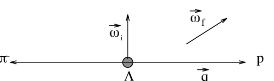
Figure 5: Kinematics of $\Lambda^{0}\rightarrow p\pi^{-}$ in the $\Lambda^{0}$ rest frame

By considering the measured branching ratios:

$$B(\Lambda^{0}\rightarrow p\pi^{-}) = 64\%$$

$$B(\Lambda^{0}\rightarrow n\pi^{0}) = 36\%,$$ (35)

and the pion-nucleon system in an isospin basis:

$$\ket{I={{1\over 2}},\;I_{3}=-{{1\over 2}}} = \sqrt{1\over 3}\ket{n\pi^{0}}-\sqrt{2\over 3}\ket{p\pi^{-}}$$

$$\ket{I={3\over 2},\;I_{3}=-{{1\over 2}}} = \sqrt{2\over 3}\ket{n\pi^{0}}+\sqrt{1\over 3}\ket{p\pi^{-}},$$ (36)

we can see that the final state is mostly an isospin $I=1/2$ state. This is the empirical result known as the $\Delta I=1/2$ rule.[23]

We first perform a model independent analysis of the decay by writing the most general matrix element consistent with Lorentz invariance:[23, 24]

$${\cal M}=G_{F}m_{\pi}^{2}\overline{U}_{P}(A-B\gamma_{5})U_{\Lambda}.$$ (37)

Because this is a two-body decay, the kinematics is fixed and $A$ and $B$ are simply constants. Other forms one could write, can be absorbed into $A$ and $B$, for example:

$$q_{\mu}\overline{U}_{P}\gamma_{\mu}U_{\Lambda}=m_{P}\overline{U}_{P}U_{\Lambda}$$ (38)

is equivalent to a contribution to $A$. The form Eq. 37 can be derived from an effective Lagrangian like:

$${\cal L}\sim\overline{\Psi}_{P}(A-B\gamma_{5})\Psi_{\Lambda}\pi.$$ (39)

Recalling the transformation properties of fermion bilinears and pions under parity:[2, 3]

$$\overline{\Psi}_{P}\Psi_{\Lambda} \stackrel{{\scriptstyle P}}{{\longrightarrow}} \overline{\Psi}_{P}\Psi_{\Lambda}$$

$$\overline{\Psi}_{P}\gamma_{5}\Psi_{\Lambda} \stackrel{{\scriptstyle P}}{{\longrightarrow}} -\overline{\Psi}_{P}\gamma_{5}\Psi_{\Lambda}$$

$$\pi \stackrel{{\scriptstyle P}}{{\longrightarrow}} -\pi,$$ (40)

one finds that

$${\cal L}\stackrel{{\scriptstyle P}}{{\longrightarrow}}\overline{\Psi}_{P}(-A-B\gamma_{5})\Psi_{\Lambda}\pi.$$ (41)

Thus, $A$ corresponds to the parity violating, $s$-wave amplitude; and $B$ to the parity conserving, $p$-wave amplitude.

To proceed, we write explicit expressions for the spinors in the $\Lambda$ rest frame:

$$U_{\Lambda}=\sqrt{2M_{\Lambda}}\left(\begin{array}[]{c}1\\ 0\end{array}\right)\chi_{i}\;\;U_{P}=\sqrt{E_{P}+M_{P}}\left(\begin{array}[]{c}1\\ {\vec{\sigma}\cdot\vec{q}\over E_{P}+M_{P}}\end{array}\right)\chi_{f}$$ (42)

where $\chi_{i,f}$ are two-component spinors. The spinor normalization is such that $\overline{U}(\vec{q},s)U(\vec{q},s^{\prime})=2M\delta_{ss^{\prime}}$. We then obtain:

$${\cal M}=G_{F}m_{\pi}^{2}\sqrt{2M_{\Lambda}(E_{P}+M_{P})}\left(A\chi^{\dagger}_{f}\chi_{i}+B\chi^{\dagger}_{f}{\vec{\sigma}\cdot\vec{q}\over E_{P}+M_{P}}\chi_{i}\right).$$ (43)

It is convenient to define:

$$\hat{q} = {\vec{q}\over|\vec{q}|}$$

$$s = A$$

$$p = {|\vec{q}|\over E_{P}+M_{P}}B$$

$$C = G_{F}m_{\pi}^{2}\sqrt{2M_{\Lambda}(E_{P}+M_{P})}.$$ (44)

In terms of these quantities we can compute the decay distribution. Squaring the matrix element:

$$|{\cal M}|^{2}=C^{2}\chi^{\dagger}_{f}(s+p\vec{\sigma}\cdot\hat{q})\chi_{i}\chi_{i}^{\dagger}(s^{*}+p^{*}\vec{\sigma}\cdot\hat{q})\chi_{f}.$$ (45)

We then make use of the projection operators:

$$\chi_{i,f}\chi^{\dagger}_{i,f}={1\over 2}(1+\vec{\sigma}\cdot\vec{\omega}_{i,f}),$$ (46)

and the identity $\sigma_{i}\sigma_{j}=\delta_{ij}+i\epsilon_{ijk}\sigma_{k}$ to find after some algebra:

$$|{\cal M}|^{2} = {|C|^{2}\over 2}\biggl{(}|s|^{2}+|p|^{2}\biggr{)}\biggl{[}1+\gamma\vec{\omega}_{i}\cdot\vec{\omega}_{f}+(1-\gamma)\hat{q}\cdot\vec{\omega}_{i}\hat{q}\cdot\vec{\omega}_{f}$$ (47)

$$+ \alpha\hat{q}\cdot(\vec{\omega}_{i}+\vec{\omega}_{f})+\beta\hat{q}\cdot(\vec{\omega}_{f}\times\vec{\omega}_{i})\biggr{]}.$$

We have introduced the notation:

$$\alpha \equiv {2{\rm Re}s^{*}p\over|s|^{2}+|p|^{2}}$$

$$\beta \equiv {2{\rm Im}s^{*}p\over|s|^{2}+|p|^{2}}$$

$$\gamma \equiv {|s|^{2}-|p|^{2}\over|s|^{2}+|p|^{2}}.$$ (48)

However, only two of these parameters are independent, since $\alpha^{2}+\beta^{2}+\gamma^{2}=1$. Sometimes one finds in the literature the parameters $\alpha$ and $\phi$, with $\beta=\sqrt{1-\alpha^{2}}\sin\phi$ and $\gamma=\sqrt{1-\alpha^{2}}\cos\phi$. The non-leptonic hyperon decay is therefore completely described by three observables: the total decay rate, and two parameters determining the angular distribution. We take the latter to be $\alpha$ and $\beta$.

The total decay rate is given by:

$$\Gamma={|\vec{q}|(E_{P}+M_{P})\over 4\pi M_{\Lambda}}G_{F}^{2}m_{\pi}^{4}\left(|s|^{2}+|p|^{2}\right).$$ (49)

One way to interpret the parameter $\alpha$ follows from considering the angular distribution in the case when the final baryon polarization is not observed:

$${d\Gamma\over d\Omega}={1\over 16\pi^{2}}{|\vec{q}|\over M_{\Lambda}}G_{F}^{2}m_{\pi}^{4}(E_{P}+M_{P})\left(|s|^{2}+|p|^{2}\right)\left(1+\alpha\hat{q}\cdot\vec{\omega}_{i}\right).$$ (50)

The polarization of the decay proton in the $\Lambda^{0}$ rest frame is given by:

$$\vec{\cal P}_{P}={1\over 1+\alpha\vec{\cal P}_{\Lambda}\cdot\hat{q}}\biggl{[}\left(\alpha+\vec{\cal P}_{\Lambda}\cdot\hat{q}\right)\hat{q}+\beta\left(\vec{\cal P}_{\Lambda}\times\hat{q}\right)+\gamma\left(\hat{q}\times\left(\vec{\cal P}_{\Lambda}\times\hat{q}\right)\right)\biggr{]}.$$ (51)

From this expression we can relate $\beta$ to the proton polarization in the direction perpendicular to the plane formed by the $\Lambda$ polarization and the proton momentum. Similarly, if the initial hyperon is unpolarized, $\alpha$ gives us the polarization of the proton. From all these expressions it is clear that $\alpha$ governs a $T$-even correlation, whereas $\beta$ governs a $T$-odd correlation. According to our general considerations, we will be able to construct a ${\cal CP}$-odd observable using the parameter $\beta$ that does not vanish in the absence of final state interactions. It will, however, be an observable extremely difficult to measure, as it will require the measurement of the polarization of both initial and final baryons. In practice, it is not possible to measure the proton polarization, so this observable is not useful for the reaction $\Lambda\rightarrow p\pi^{-}$. However, if one studies the decay chain:

$$\Xi^{-}\rightarrow\Lambda^{0}\pi^{-}\rightarrow p\pi^{-}\pi^{-}$$ (52)

it is possible to study the correlation that gives $\beta_{\Xi}$, since the polarization of the final baryon (in this case the $\Lambda$) can be obtained by analyzing the angular distribution of the second decay.

5.1 $\not\!\!{\cal CP}$ and unitarity phases

Even though we are discussing weak decays, the final state consists of strongly interacting particles, so there will be strong rescattering phases. These phases are responsible for the non-zero value of $\beta$ even in the absence of ${\cal CP}$ violation, in accordance with Eq. 12. It is convenient to analyze the final pion-nucleon system in terms of isospin and parity eigenstates. In that way we can have in mind the simple picture:

$$\Lambda^{0}\stackrel{{\scriptstyle H_{W}}}{{\longrightarrow}}\bigg{(}p\pi\bigg{)}^{I}_{\ell}\stackrel{{\scriptstyle H_{S}}}{{\longrightarrow}}\bigg{(}p\pi\bigg{)}^{I}_{\ell}.$$ (53)

At $t=0$ the weak Hamiltonian induces the decay of the $\Lambda^{0}$ into a pion-nucleon system with isospin and parity given by $I,~{}\ell$. This pion-nucleon system is then an eigenstate of the strong interaction. Furthermore, at an energy equal to the $\Lambda$ mass, it is the only state with these quantum numbers. The pion-nucleon system will then rescatter due to the strong interactions into itself, and in the process pick up a phase $\delta^{I}_{\ell}$. This is an example of what is known as Watson’s theorem, and an excellent discussion can be found in T.D.Lee’s book [1]. We reproduce here the main steps in the proof[1]. The matrix elements that we need are, to lowest order in the weak interactions:

$$A^{I}_{\ell}=\left<(p\pi)^{I}_{\ell}\right|H_{W}\left|\Lambda^{0}\right>_{m}.$$ (54)

Both states are eigenstates of angular momentum with $J={1\over 2}$ and $J_{z}=m$, but rotational invariance implies that this matrix element is independent of the quantum number $m$, so we will drop that subscript. The time evolution of the final state due to the strong interactions is given by:

$$\ket{(p\pi)^{I}_{\ell}}=U^{\dagger}_{S}(\infty,0)\ket{(p\pi)^{I}_{\ell},{\rm free}}.$$ (55)

Replacing Eq. 55 into Eq. 54, taking the complex conjugate, introducing several factors of $1=U^{\dagger}_{T}U_{T}$, and finally using Eq. 7:

$$A^{I}_{\ell} = \left<(p\pi)^{I}_{\ell},{\rm free}\right|U_{S}(\infty,0)H_{W}(0)\left|\Lambda^{0}\right>$$

$$A^{I*}_{\ell} = \bra{(p\pi)^{I}_{\ell},{\rm free}}^{*}U_{S}^{*}(\infty,0)H_{W}^{*}(0)\ket{\Lambda^{0}}^{*}$$ (56)

$$= \bra{(p\pi)^{I}_{\ell},{\rm free}}^{*}U^{\dagger}_{T}\left(U_{T}U_{S}^{*}(\infty,0)U_{T}^{\dagger}\right)\left(U_{T}H_{W}^{*}(0)U^{\dagger}_{T}\right)U_{T}\ket{\Lambda^{0}}^{*}$$

$$= \left<(p\pi)^{I}_{\ell},{\rm free}\right|{\cal T}^{-1}\left({\cal T}U_{S}(\infty,0){\cal T}^{-1}\right)\left({\cal T}H_{W}(0){\cal T}^{-1}\right){\cal T}\left|\Lambda^{0}\right>.$$

But we know that angular momentum eigenstates transform according to Eq. 5, so:

$${\cal T}\ket{\Lambda^{0}} = (-)^{{1\over 2}+m}\ket{\Lambda^{0}}_{-m}$$

$${\cal T}\ket{(p\pi)^{I}_{\ell},{\rm free}}_{m} = (-)^{{1\over 2}+m}\ket{(p\pi)^{I}_{\ell},{\rm free}}_{-m}.$$ (57)

Assuming time reversal invariance of both the strong and weak interactions we thus find:

$$A^{I*}_{\ell}=\left<(p\pi)^{I}_{\ell},{\rm free}\right|U_{S}(-\infty,0)H_{W}(0)\left|\Lambda^{0}\right>_{-m}.$$ (58)

Again, due to rotational invariance, we can drop the $-m$ subindex.We can also use

$$U_{S}(-\infty,0)=U_{S}(-\infty,\infty)U_{S}(\infty,0)=S^{\dagger}U_{S}(\infty,0)$$ (59)

to finally obtain:

$$A^{I*}_{\ell} = \left<(p\pi)^{I}_{\ell},{\rm free}\right|S^{\dagger}U_{S}(\infty,0)H_{W}(0)\left|\Lambda^{0}\right>$$ (60)

$$= \sum_{n}\left<(p\pi)^{I}_{\ell},{\rm free}\right|S^{\dagger}\left|n\right>\left<n\right|U_{S}(\infty,0)H_{W}(0)\left|\Lambda^{0}\right>.$$

However, we have argued that at an energy equal to the $\Lambda^{0}$ mass, the $p\pi$ state is the only state with quantum numbers $I,\ell$. The $S$-matrix element, thus, vanishes for all elements of the sum except for the case where the intermediate state is the same as the final state, in which case it is just equal to the strong phase shift

$$\left<(p\pi)^{I}_{\ell},{\rm free}\right|S^{\dagger}\left|(p\pi)^{I}_{\ell},{\rm free}\right>=e^{-2i\delta^{I}_{\ell}},$$ (61)

and thus

$$A^{I*}_{\ell}=e^{-2i\delta^{I}_{\ell}}A^{I}_{\ell}.$$ (62)

This completes the proof of the statement that in the absence of ${\cal CP}$ violation, the phase of the decay amplitude is equal to the strong rescattering phase of the final state. You already saw a similar result in the analysis of the parameters $\epsilon$ and $\epsilon^{\prime}$ in kaon decays.[7]

Getting back to our problem, we can write the matrix elements for the different isospin and parity channels as:

$$s = s_{1}e^{i(\delta^{1}_{s}+\phi^{1}_{s})}+s_{3}e^{i(\delta^{3}_{s}+\phi^{3}_{s})}$$

$$p = p_{1}e^{i(\delta^{1}_{p}+\phi^{1}_{p})}+p_{3}e^{i(\delta^{3}_{p}+\phi^{3}_{p})},$$ (63)

where the notation is such that: the indices $1,3$ refer to isospin $1/2,3/2$ final states; $\delta$ are the strong rescattering phases; and $\phi$ are possible ${\cal CP}$ violating phases. In this example, the final state with isospin $1/2$, $3/2$ can only be reached via the $\Delta I=1/2,3/2$ parts of the weak Hamiltonian. According to the $\Delta I=1/2$ rule, therefore, the final state is predominantly an isospin $1/2$ state.

We now relate this decay to the corresponding anti-particle decay $\overline{\Lambda}^{0}\rightarrow\overline{p}\pi^{+}$. To do this, we repeat the analysis used to prove Watson’s theorem, but without assuming time reversal invariance of the weak interactions. We find:

$$A^{I*}_{\ell} = e^{-2i\delta^{I}_{\ell}}\left<(p\pi)^{I}_{\ell}\right|{\cal T}H_{W}{\cal T}^{-1}\left|\Lambda\right>$$ (64)

$$= e^{-2i\delta^{I}_{\ell}}\left<(p\pi)^{I}_{\ell}\right|({\cal CP})^{-1}({\cal CP}{\cal T})H_{W}({\cal CP}{\cal T})^{-1}({\cal CP})\left|\Lambda\right>$$

We now assume ${\cal CP}{\cal T}$ invariance of the weak interactions to find:

$$A^{I*}_{\ell}=e^{-2i\delta^{I}_{\ell}}\left<(p\pi)^{I}_{\ell}\right|({\cal CP})^{-1}H_{W}({\cal CP})\left|\Lambda\right>$$ (65)

The next step involves a choice of ${\cal CP}$ phases. It is easy to convince yourself that the physics does not depend on this choice, although intermediate steps might look different. We choose, in accordance with Eq. 2:

$${\cal CP}\ket{\Lambda} = \ket{\overline{\Lambda}}$$

$${\cal CP}\ket{(p\pi)^{I}_{\ell}} = -(-)^{\ell}\ket{(p\pi)^{I}_{\ell}}.$$ (66)

Defining the amplitudes for the anti-lambda decay via the notation

$$\overline{A}^{I}_{\ell}\equiv\left<(\overline{p}\pi)^{I}_{\ell}\right|H_{W}\left|\overline{\Lambda}\right>$$ (67)

we then find[23]:

$$A^{I*}_{\ell}=-(-)^{\ell}\overline{A}^{I}_{\ell}e^{-2i\delta^{I}_{\ell}}.$$ (68)

If, on the other hand, we assume ${\cal CP}$ invariance of the weak Hamiltonian, we are led to

$$A^{I}_{\ell}=\left<(p\pi)^{I}_{\ell}\right|({\cal CP})^{-1}\left({\cal CP}H_{W}{\cal CP}^{-1}\right)({\cal CP})\left|\Lambda\right>.$$ (69)

With the same phase convention as above, we thus find that ${\cal CP}$ invariance would predict[23]:

$$A^{I}_{\ell}=-(-)^{\ell}\overline{A}^{I}_{\ell}.$$ (70)

If we parameterize the amplitudes in non-leptonic hyperon decays as:

$$S=\sum_{I}s_{I}e^{i(\delta^{I}_{s}+\phi^{I}_{s})}\;\;P=\sum_{I}p_{I}e^{i(\delta^{I}_{p}+\phi^{I}_{p})},$$ (71)

then ${\cal CP}{\cal T}$ invariance of the weak Hamiltonian predicts:[25]

$$\overline{S}=\sum_{I}-s_{I}e^{i(\delta^{I}_{s}-\phi^{I}_{s})}\;\;\overline{P}=\sum_{I}p_{I}e^{i(\delta^{I}_{p}-\phi^{I}_{p})},$$ (72)

whereas ${\cal CP}$ invariance of the weak interactions predicts:

$$\overline{S}=\sum_{I}-s_{I}e^{i(\delta^{I}_{s}+\phi^{I}_{s})}\;\;\overline{P}=\sum_{I}p_{I}e^{i(\delta^{I}_{p}+\phi^{I}_{p})}.$$ (73)

From this we see again that the $\phi^{I}_{\ell}$ phases violate ${\cal CP}$. Our task now, is to compare the hyperon and anti-hyperon decay to construct ${\cal CP}$ odd observables to extract $\phi^{I}_{\ell}$.

Once again we emphasize that

$$\beta={2{\rm Im}s^{*}p\over|s|^{2}+|p|^{2}}\not=0$$ (74)

even if ${\cal CP}$ is conserved. In our previous language, a (naive)-$T$-odd observable is not a ${\cal CP}$ or ${\cal T}$ odd observable.

5.2 Observables

With the expressions of the previous section, we can compute the three observables for the decay $\Lambda^{0}\rightarrow p\pi^{-}$:

$$\Gamma = {|\vec{q}|C^{2}\over 8\pi M_{\Lambda}^{2}}\biggl{\{}\sum_{I}\left(|s_{I}|^{2}+|p_{I}|^{2}\right)$$

$$+ \sum_{I\not=J}2s_{I}s_{J}\left[\cos(\phi^{I}_{s}-\phi^{J}_{s})\cos(\delta^{I}_{s}-\delta^{J}_{s})-\sin(\phi^{I}_{s}-\phi^{J}_{s})\sin(\delta^{I}_{s}-\delta^{J}_{s})\right]$$

$$+ \sum_{I\not=J}2p_{I}p_{J}\left[\cos(\phi^{I}_{p}-\phi^{J}_{p})\cos(\delta^{I}_{p}-\delta^{J}_{p})-\sin(\phi^{I}_{p}-\phi^{J}_{p})\sin(\delta^{I}_{p}-\delta^{J}_{p})\right]\biggr{\}}$$

$$\alpha\Gamma = {|\vec{q}|C^{2}\over 4\pi M_{\Lambda}^{2}}\sum_{I,J}s_{I}p_{J}\left[\cos(\phi^{I}_{s}-\phi^{J}_{p})\cos(\delta^{I}_{s}-\delta^{J}_{p})-\sin(\phi^{I}_{s}-\phi^{J}_{p})\sin(\delta^{I}_{s}-\delta^{J}_{p})\right]$$

$$\beta\Gamma = {|\vec{q}|C^{2}\over 4\pi M_{\Lambda}^{2}}\sum_{I,J}s_{I}p_{J}\left[\sin(\phi^{I}_{s}-\phi^{J}_{p})\cos(\delta^{I}_{s}-\delta^{J}_{p})+\cos(\phi^{I}_{s}-\phi^{J}_{p})\sin(\delta^{I}_{s}-\delta^{J}_{p})\right]$$ (75)

whereas for the $\overline{\Lambda}^{0}\rightarrow\overline{p}\pi^{+}$ decay we find:

$$\overline{\Gamma} = {|\vec{q}|C^{2}\over 8\pi M_{\Lambda}^{2}}\biggl{\{}\sum_{I}\left(|s_{I}|^{2}+|p_{I}|^{2}\right)$$

$$+ \sum_{I\not=J}2s_{I}s_{J}\left[\cos(\phi^{I}_{s}-\phi^{J}_{s})\cos(\delta^{I}_{s}-\delta^{J}_{s})+\sin(\phi^{I}_{s}-\phi^{J}_{s})\sin(\delta^{I}_{s}-\delta^{J}_{s})\right]$$

$$+ \sum_{I\not=J}2p_{I}p_{J}\left[\cos(\phi^{I}_{p}-\phi^{J}_{p})\cos(\delta^{I}_{p}-\delta^{J}_{p})+\sin(\phi^{I}_{p}-\phi^{J}_{p})\sin(\delta^{I}_{p}-\delta^{J}_{p})\right]\biggr{\}}$$

$$\overline{\alpha}\overline{\Gamma} = -{|\vec{q}|C^{2}\over 4\pi M_{\Lambda}^{2}}\sum_{I,J}s_{I}p_{J}\left[\cos(\phi^{I}_{s}-\phi^{J}_{p})\cos(\delta^{I}_{s}-\delta^{J}_{p})+\sin(\phi^{I}_{s}-\phi^{J}_{p})\sin(\delta^{I}_{s}-\delta^{J}_{p})\right]$$

$$\overline{\beta}\overline{\Gamma} = {|\vec{q}|C^{2}\over 4\pi M_{\Lambda}^{2}}\sum_{I,J}s_{I}p_{J}\left[\sin(\phi^{I}_{s}-\phi^{J}_{p})\cos(\delta^{I}_{s}-\delta^{J}_{p})-\cos(\phi^{I}_{s}-\phi^{J}_{p})\sin(\delta^{I}_{s}-\delta^{J}_{p})\right]$$ (76)

Comparing these expressions, we can construct the three ${\cal CP}$-odd observables:[26, 27]

$$\Delta \equiv {\Gamma-\overline{\Gamma}\over\Gamma+\overline{\Gamma}}$$

$$A \equiv {\alpha\Gamma+\overline{\alpha}\overline{\Gamma}\over\alpha\Gamma-\overline{\alpha}\overline{\Gamma}}=-{\sum_{I,J}s_{I}p_{J}\sin(\phi^{I}_{s}-\phi^{J}_{p})\sin(\delta^{I}_{s}-\delta^{J}_{p})\over\sum_{I,J}s_{I}p_{J}\cos(\phi^{I}_{s}-\phi^{J}_{p})\cos(\delta^{I}_{s}-\delta^{J}_{p})}$$

$$B \equiv {\beta\Gamma+\overline{\beta}\overline{\Gamma}\over\beta\Gamma-\overline{\beta}\overline{\Gamma}}=-{\sum_{I,J}s_{I}p_{J}\sin(\phi^{I}_{s}-\phi^{J}_{p})\cos(\delta^{I}_{s}-\delta^{J}_{p})\over\sum_{I,J}s_{I}p_{J}\cos(\phi^{I}_{s}-\phi^{J}_{p})\sin(\delta^{I}_{s}-\delta^{J}_{p})}$$ (77)

It is, perhaps, more useful to construct approximate expressions based on the fact that there are three small parameters in the problem:

• The strong rescattering phases are measured to be small.

• The $\Delta I=3/2$ amplitudes are much smaller than the $\Delta I=1/2$ amplitudes.

• The ${\cal CP}$ violating phases are small.

To leading order in all the small quantities one finds:[27]

$$\Delta = \sqrt{2}{s_{3}\over s_{1}}\sin\left(\delta_{s}^{3}-\delta_{s}^{1}\right)\sin\left(\phi_{s}^{3}-\phi_{s}^{1}\right)$$

$$A = -\tan\left(\delta_{p}^{1}-\delta_{s}^{1}\right)\sin\left(\phi_{p}^{1}-\phi_{s}^{1}\right)$$

$$B = -\cot\left(\delta_{p}^{1}-\delta_{s}^{1}\right)\sin\left(\phi_{p}^{1}-\phi_{s}^{1}\right)$$ (78)

We can see in these expressions that $\Delta$ arises mainly from an interference between a $\Delta I=1/2$ and a $\Delta I=3/2$ $s$-waves, and that it is suppressed by three small quantities. On the other hand, $A$ arises as an interference of $s$ and $p$-waves of the same isospin and, therefore, it is not suppressed by the $\Delta I=1/2$ rule. Finally, we can see that $B$ is not suppressed by the small rescattering phases. This is as we expected for a ${\cal CP}$ odd observable that is also (naive)-$T$ odd. The hierarchy $B>>A>>\Delta$ emerges.[26]

This is as far as we can go in a model independent manner. If we want to predict the value of these observables within a model for ${\cal CP}$ violation we take the value of $s_{3}/s_{1}$ and the strong rescattering phases from experiment and we try to compute the weak phases from theory.

5.3 Standard model calculation

In the case of the minimal standard model, the ${\cal CP}$ violating phase resides in the CKM matrix. For low energy transitions, this phase shows up as the imaginary part of the Wilson coefficients in the effective weak Hamiltonian.[28] In the notation of Buras [9],

$$H_{W}^{eff} = {G_{F}\over\sqrt{2}}V^{*}_{ud}V_{us}\sum_{i}c_{i}(\mu)Q_{i}(\mu)+{\rm~{}hermitian~{}conjugate}$$

$$Q_{1} = (\overline{s}d)_{V-A}(\overline{u}u)_{V-A}$$

$$Q_{2} = (\overline{s}u)_{V-A}(\overline{u}d)_{V-A}$$

$$Q_{3} = (\overline{s}d)_{V-A}\sum_{q=u,d,s}(\overline{q}q)_{V-A}$$

$$Q_{5} = (\overline{s}d)_{V-A}\sum_{q=u,d,s}(\overline{q}q)_{V+A}$$

$$Q_{6} = -8\sum_{q=u,d,s}(\overline{s}_{L}q_{R})(\overline{q}_{R}d_{L})$$

$$Q_{7} = {3\over 2}(\overline{s}d)_{V-A}\sum_{q=u,d,s}e_{q}(\overline{q}q)_{V+A}$$

$$Q_{8} = -12\sum_{q=u,d,s}e_{q}(\overline{s}_{L}q_{R})(\overline{q}_{R}d_{L})$$ (79)

The origin of the different terms in this Hamiltonian was discussed in the lectures by De Rafael. Here, I just remind you that the Wilson coefficients are typically written as

$$c_{i}(\mu) = z_{i}(\mu)+\tau y_{i}(\mu)$$

$$\tau = -{V^{*}_{td}V_{ts}\over V^{*}_{ud}V_{us}}$$ (80)

and the ${\cal CP}$ violating phase is the phase of $\tau$. Numerical values for these coefficients can be found, for example, in Buchalla et. al..[29]

The calculation would proceed as usual, by evaluating the hadronic matrix elements of the four-quark operators in Eq. 79 to obtain real and imaginary parts for the amplitudes, schematically:

$$\left<p\pi\right|H_{w}^{eff}\left|\Lambda^{0}\right>|^{I}_{\ell}={\rm Re}M^{I}_{\ell}+i{\rm Im}M^{I}_{\ell},$$ (81)

and to the extent that the ${\cal CP}$ violating phases are small, they can be approximated by

$$\phi^{I}_{\ell}\approx{{\rm Im}M^{I}_{\ell}\over{\rm Re}M^{I}_{\ell}}.$$ (82)

At present, however, we do not know how to compute the matrix elements so we cannot actually implement this calculation. If we try to follow what is done for kaon decays, we would compute the matrix elements using factorization and vacuum saturation as a reference point, then define some parameters analogous to $B_{K}$ that would measure the deviation of the matrix elements from their vacuum saturation value. A reliable calculation of the “$B$” parameters would probably have to come from lattice QCD.

For a simple estimate, we can take the real part of the matrix elements from experiment (assuming that the measured amplitudes are real, that is, that ${\cal CP}$ violation is small), and compute the imaginary parts in vacuum saturation. Since the vacuum saturation result is much smaller than the measured amplitudes, this provides a conservative estimate for the weak phases. There are many models in the literature that claim to fit the experimentally measured amplitudes. Without entering into the details of these models, it is obvious that to fit the data, the models must enhance some or all of the matrix elements with respect to vacuum saturation. Clearly, one would get completely different phases depending on which matrix elements are enhanced. It is not surprising, therefore, that a survey of these models yields weak $\not\!\!{\cal CP}$ phases that differ by an order of magnitude[30].

To compute some numbers, we take from experiment:[31, 32]

$${s_{3}\over s_{1}} = -0.019\pm 0.006$$

$$\delta^{1}_{s}=6^{\circ} \delta^{3}_{s}=-3.8^{\circ}$$

$$\delta^{1}_{p}=-1.1^{\circ} \delta^{3}_{p}=-0.7^{\circ}$$ (83)

and the approximate weak phases estimated in vacuum saturation:[30]

$$\phi^{1}_{s} \approx -3y_{6}{\rm Im}\tau$$

$$\phi^{1}_{p} \approx -0.3y_{6}{\rm Im}\tau$$

$$\phi^{3}_{s} \approx \left[3.56(y_{1}+y_{2})+4.1(y_{7}+2y_{8}){m_{\pi}^{2}\over m_{s}(m_{u}+m_{d})}\right]{\rm Im}\tau$$ (84)

To get some numerical estimates we use the values for the Wilson coefficients of Buchalla et. al.[29] with $\mu=1$ GeV, $\Lambda_{QCD}=200$ MeV. Although quantities such as the quark masses that appear in Eq. 84 are not physical[33], we will use for an estimate the value $m_{\pi}^{2}/(m_{s}(m_{u}+m_{d}))\sim 10$. For the quantity ${\rm Im}\tau$ we use the upper bound from Eq. 14, ${\rm Im}\tau\leq 0.0014$. With all this we find:

$$\Delta = \left\{\begin{array}[]{ll}-1.4\times 10^{-6}&{\rm~{}for~{}}m_{t}=150~{}GeV\\ -9.1\times 10^{-7}&{\rm~{}for~{}}m_{t}=200~{}GeV\end{array}\right.$$ (87)

$$A = 3.7\times 10^{-5}$$

$$B = 2.4\times 10^{-3}$$ (88)

A survey of several models for the hadronic matrix elements, combined with a careful analysis of the allowed range for the short distance parameters that enter the calculation yielded similar results: that $A$ was in the range of ${\rm``a~{}few"~{}}\times 10^{-5}$ and that $\Delta$ was two orders of magnitude smaller. The rate asymmetry exhibits a strong dependence on the top-quark mass: for a certain value of $m_{t}$, the two terms in Eq. 84 cancel against each other. The angular correlation asymmetries, on the other hand, depend mildly on the top-quark mass. This is understood from the point of view that the most important effect of a large top-quark mass is to enhance electroweak corrections to the effective weak Hamiltonian. This is important for the $\Delta I=3/2$ amplitudes but not for the $\Delta I=1/2$ amplitudes.

6 ${\cal CP}$-violating effective Lagrangian

In this section we show a few examples of ${\cal CP}$ violating new physics that can be discussed in terms of a low energy effective interaction. We use these interactions in the following section to estimate bounds that different observables can place on the new physics. An extensive list of $\not\!\!{\cal CP}$ operators compatible with the symmetries of the standard model has been given by Burgess and Robinson.[19] The importance of requiring the effective operators to be gauge invariant has been emphasized by de Rújula and collaborators.[34]

6.1 Operators that can appear at tree-level

An example of heavy particle exchange at tree-level, that results in a ${\cal CP}$ violating effective Lagrangian is that shown in Figure 6.

Figure 6: ${\cal CP}$ violating operators at tree-level.

Evaluating the diagram in Figure 6 with the couplings of Eq. 32 we find:

$${\cal M}=\left(-{m_{t}\over v}\right)^{2}\overline{t}\left({\rm Re}A-i{\rm Im}A\gamma_{5}\right)t\overline{t}\left({\rm Re}A-i{\rm Im}A\gamma_{5}\right)t{i\over q^{2}-M^{2}_{H}}.$$ (89)

In the heavy mass limit, this matrix element can be derived from the effective interaction:

$${\cal L}^{\not\!\!{\cal CP}}_{eff}=i\sqrt{2}\left({m_{t}\over v}\right)^{2}{1\over M_{H}^{2}}\overline{t}\gamma_{5}t\overline{t}t.$$ (90)

where we have assumed the unitarity upper bound for the $\not\!\!{\cal CP}$ coupling. Similarly, we can write down interactions like:

$${\cal L}^{\not\!\!{\cal CP}}_{eff}=i\overline{\eta}{g^{2}\over\Lambda^{2}}\overline{d}u\overline{t}\gamma_{5}b+{\rm~{}h.~{}c.}$$ (91)

obtained after Fierzing the operator that arises from an $s$-channel exchange of a charged scalar of mass $\Lambda$ that couples with strength $g$ and $\not\!\!{\cal CP}$ mixing angles $\overline{\eta}$.

6.2 One-loop effective operators: dipole moments

One of the most commonly studied $\not\!\!{\cal CP}$ operators that can appear at one-loop is the electric-dipole moment of a fermion and its generalizations to weak and strong couplings. The most general matrix element of the electromagnetic current between two spinors contains a ${\cal T}$-odd term:

$$\left<\Psi\right|j^{em}_{\mu}\left|\Psi\right>=iF_{3}(q^{2})\overline{U}(p_{2})\sigma_{\mu\nu}q^{\nu}\gamma_{5}U(p_{1}).$$ (92)

The value of this form factor at zero-momentum transfer:

$$F_{3}(q^{2}=0)\equiv d^{\gamma}_{\Psi}$$ (93)

is called the electric-dipole-moment. This induces a local interaction that can be derived form the effective Lagrangian:

$${\cal L}^{d}_{eff} = {1\over 2}d_{f}^{\gamma}\overline{\Psi}_{f}i\sigma_{\mu\nu}\gamma_{5}\Psi_{f}F^{\mu\nu}$$ (94)

$$+ {1\over 2}d_{f}^{Z}\overline{\Psi}_{f}i\sigma_{\mu\nu}\gamma_{5}\Psi_{f}Z^{\mu\nu}$$

$$+ {1\over 2}d_{f}^{g}\overline{\Psi}_{f}i\sigma_{\mu\nu}\gamma_{5}{\lambda_{a}\over 2}\Psi_{f}G^{\mu\nu}_{a}$$

where we have also added the generalizations to fermion couplings to the $Z$ boson and gluons.

Recalling that $\sigma_{\mu\nu}\gamma_{5}=(i/2)\epsilon_{\mu\nu\rho\sigma}\sigma^{\rho\sigma}$, it is easy to prove that this interaction is indeed ${\cal P}$ and ${\cal T}$ odd. Under parity:

$${\cal P}A^{\mu}{\cal P}^{-1}=A_{\mu} {\cal P}\partial^{\mu}{\cal P}^{-1}=\partial_{\mu}$$

$${\cal P}F^{\mu\nu}{\cal P}^{-1}=F_{\mu\nu} {\cal P}:\overline{\Psi}\sigma^{\mu\nu}\Psi:{\cal P}^{-1}=:\overline{\Psi}\sigma_{\mu\nu}\Psi:$$ (95)

and under time reversal invariance:

$${\cal T}A^{\mu}{\cal T}^{-1}=A_{\mu} {\cal T}\partial^{\mu}{\cal T}^{-1}=-\partial_{\mu}$$

$${\cal T}F^{\mu\nu}{\cal T}^{-1}=-F_{\mu\nu} {\cal T}:\overline{\Psi}\sigma^{\mu\nu}\Psi:{\cal T}^{-1}=-:\overline{\Psi}\sigma_{\mu\nu}\Psi:$$ (96)

using $\epsilon^{\mu\nu\rho\sigma}=-\epsilon_{\mu\nu\rho\sigma}$ it then follows that $d^{\gamma}_{f}$ is odd under both ${\cal P}$ and ${\cal T}$.

In the minimal standard model the electric dipole moment of a quark vanishes at the one-loop order. Diagrams that might contribute are shown in Figure 7, where it is seen that at one-loop there can be no $\not\!\!{\cal CP}$ phase.[35]

Figure 7: Potential contributions to a quark edm in the standard model at one loop.

Diagrams at two-loop order can have a $\not\!\!{\cal CP}$ phase, but it has been shown by Shabalin [36] that the sum of two-loop contributions to $F_{3}(q^{2}=0)$ vanishes. It is thus thought that in the standard model, the lowest order contribution to the quark electric dipole moment occurs at the three-loop level.

As an aside, it is worth commenting that the electric dipole moment of the neutron is a much more complicated quantity to calculate (as in many other cases the complication arises in computing the hadronic matrix elements of quark operators). It seems, however, that the value of the neutron EDM in the standard model is many orders of magnitude below the current experimental upper bound.[37] It has been claimed that it can be as large as $10^{-30}$ e-cm,[38] although more likely values are at the $10^{-33}$ e-cm level.[39] Recall that the experimental results for the neutron and electron edm are:

$$d_{n}^{\gamma} = (-1.4\pm 0.6)\times 10^{-25}{\rm e-cm}$$

$$d_{n}^{\gamma} = (-0.3\pm 0.5)\times 10^{-25}{\rm e-cm}$$

$$d_{e}^{\gamma} = (-2.7\pm 8.3)\times 10^{-27}{\rm e-cm}$$ (97)

where the numbers come respectively from experiments at Leningrad,[40] Grenoble,[41] and LBL.[42].

There are models where it is possible to obtain a non-zero quark electric-dipole moment at the one-loop level. Examples are the models of $\not\!\!{\cal CP}$ with extra scalars. In the case where the ${\cal CP}$ violation arises in the charged scalar sector, the electric-dipole moment is generated by the diagrams in Figure 8.

Figure 8: Quark edm from charged Higgs at one-loop.

For down-type quarks, one obtains:[43]

$$d_{D}^{\gamma}=e{\sqrt{2}G_{F}\over 12\pi^{2}}m_{D}{\rm Im}\alpha_{1}\beta_{1}^{*}\left|V_{td}^{*}\right|{x_{t}\over(1-x_{t})^{2}}\left({3\over 4}-{5\over 4}x_{t}+{1-{3\over 2}x_{t}\over 1-x_{t}}\log x_{t}\right)$$ (98)

where $x_{t}=m_{t}^{2}/M_{H}^{2}$. This result follows from the dominance of the top-quark in the loop and assumes that the dominant contribution comes from the lightest charged scalar $H^{+}$. For the case of an up-type quark the result is:[43]

$$d_{U}^{\gamma}=e{\sqrt{2}G_{F}\over 12\pi^{2}}m_{U}{\rm Im}\alpha_{1}\beta_{1}^{*}\sum_{i}\left|V_{ui}\right|^{2}{x_{i}\over(1-x_{i})^{2}}\left(x_{i}-{1-3x_{i}\over 2(1-x_{i})}\log x_{i}\right)$$ (99)

which is much smaller than the electric dipole moment of down-type quarks due to the small masses of the quarks in the loop.

When ${\cal CP}$ violation comes from the exchange of a neutral Higgs, the quark electric-dipole moment arises through the diagram of Figure 9.

Figure 9: Fermion edm from neutral Higgs at one-loop.

In this case the value for up-type quarks,down-type quarks, or charged leptons is given in the $M_{H}>>m_{f}$ limit by:[44]

$$d_{f}^{\gamma}={eQ_{f}\sqrt{2}G_{F}\over 32\pi^{2}}m_{f}^{3}{{\rm Im}A{\rm Re}A\over M_{H}^{2}}\log\left({m_{H}^{2}\over M_{f}^{2}}\right).$$ (100)

This is largest for the top-quark (although in the case of the top-quark it may be a poor approximation to take $q^{2}=0$).

There are several new features that arise at high energy, for example, in the generalization of the electric-dipole moments to couplings to the $Z$-boson. For example, if $q^{2}=0$ is not a good approximation, and the full form factor is important, it is possible to have absorptive phases as shown schematically in Figure 10.

Figure 10: Possible absorptive phase in $d^{Z}_{q}$.

In this one-loop diagram, for $q^{2}>>4m_{f}^{2}$ the size of the imaginary and real parts is comparable. In this type of problems there is, therefore, no “penalty” associated with ${\cal CP}$-odd observables that need unitarity phases, unlike previous examples. In the limit $m_{q}<<M_{Z}$, the diagram of Figure 10 generates a $Z$-dipole moment:

$$d_{q}^{Z}(q^{2}=M_{Z}^{2}) = -{g\over 4\cos\theta_{W}}{g_{V}\over 16\pi^{2}v^{2}}{\rm Re}A{\rm Im}A{m_{q}^{3}\over M_{Z}^{2}}$$ (101)

$$\cdot\left[{\rm Li}_{2}\left(-{q^{2}\over M_{H}^{2}}\right)+\log\left(-{q^{2}\over M_{H}^{2}}\right)\log\left(1+{q^{2}\over M_{H}^{2}}\right)\right]$$

Using, as always, the unitarity upper bound for the $\not\!\!{\cal CP}$ phase, this gives

$${\rm Im}d^{Z}_{b}\approx{g\over 4\cos\theta_{W}}\left\{\begin{array}[]{ll}10^{-8}~{}GeV^{-1}\sim 10^{-22}{\rm e-cm}&{\rm~{}if~{}}M_{H}=M_{Z}\\ 10^{-10}~{}GeV^{-1}\sim 10^{-24}{\rm e-cm}&{\rm~{}if~{}}M_{H}=10M_{Z}\end{array}\right.$$ (102)

As an aside, it is interesting to understand the origin of the absorptive part of the dipole moments in the effective Lagrangian formalism, where the couplings are really constants and not form factors. The same interaction that generates the dipole moment at one-loop, generates a $\not\!\!{\cal CP}$ four fermion operator at tree-level as in Eq. 90. In the effective theory calculation at one-loop, one must include both the tree-level $Z\rightarrow\overline{f}f$ graph with the $d^{Z}_{f}$ vertex, and the one-loop graph with a $Z\rightarrow\overline{f}f$ standard model vertex followed by a $\not\!\!{\cal CP}$ four fermion vertex. It is this second diagram that contains the absorptive part.

7 ${\cal CP}$-odd observables that probe $d^{\gamma,Z,g}_{f}$

In this section we consider several observables that can be used to place bounds on the couplings $d^{\gamma,Z,g}_{f}$.

7.1 ${\cal CP}$-even observable

The existence of a new coupling, even if it is a ${\cal CP}$-violating one, changes the cross-section fermion pair production. By measuring this cross-section precisely, one can place bounds on its deviations from minimal standard model predictions and, thus, on new couplings like the dipole moments. Barr and Marciano used this method to place bounds on the electric dipole moment of the $\tau$.[37] At PETRA energies, $\sqrt{s}=35$ GeV, the process $e^{+}e^{-}\rightarrow\tau^{+}\tau^{-}$ is dominated by photon exchange. The cross-section from standard model and electric-dipole moment couplings is given by:[37]

$$\sigma={4\pi\alpha^{2}\over 3s}\left(1-{4m_{\tau}^{2}\over s}\right)^{1\over 2}\left(1+{2m_{\tau}^{2}\over s}\right)\left[1+{s\over 2}\left({d^{\gamma}_{\tau}\over e}\right)^{2}\left(1-{4m_{\tau}^{2}\over s}\right)\left(1+{2m_{\tau}^{2}\over s}\right)^{-1}\right]$$ (103)

Since no deviations from the standard model have been observed, Barr and Marciano found that $|d^{\gamma}_{\tau}|\leq 1.3\times 10^{-16}$ e-cm by assuming that the cross-section can be measured to $5\%$. In order to asses the significance of this bound, consider the case of ${\cal CP}$ violation by exchange of a neutral Higgs boson, Eq. 100. Using the unitarity upper bound for the $\not\!\!{\cal CP}$ phases, Eq. 33, this gives $d_{\tau}^{\gamma}\sim 10^{-23}$ e-cm. The same formula, Eq. 100, applied to the electron gives $d^{\gamma}_{e}\sim 10^{-33}$ e-cm, which is also much smaller than the current experimental bound, Eq. 97.

7.2 ${\cal CP}$-even angular distribution

It was shown by Del Aguila and Sher [45], that the differential cross-section is also sensitive to the presence of an electric-dipole moment of the tau. In this case, one does not have to assume a future precision measurement of the cross-section, but can actually use what has been measured by PETRA. The result is:[45]

$${d\sigma\over d(\cos\theta)} = {\pi\alpha^{2}\over 2s}\left[1+\cos^{2}\theta+{1\over 4\sin^{2}\theta_{W}\cos^{2}\theta_{W}}{\rm Re}{s\over s-M_{Z}^{2}+i{\Gamma_{Z}\over M_{Z}}}\right]$$ (104)

$$+ {1\over 2}\pi\alpha^{2}\left({d^{\gamma}_{\tau}\over e}\right)^{2}\sin^{2}\theta,$$

Fitting the PETRA results for $\sqrt{s}=35$ GeV at the $1\sigma$ level, the bound $|d^{\gamma}_{\tau}|\leq 1.4\times 10^{-16}$ e-cm is obtained.[45]

7.3 ${\cal CP}$-odd angular correlations

If we ignore the possibility of absorptive phases in the dipole-moment form factors, and simply take $d^{\gamma}_{\tau}$ to be a constant, the largest absorptive phases present in the reaction $e^{+}e^{-}\rightarrow\tau^{+}\tau^{-}$ come from the $Z$ width and are proportional to $\Gamma_{Z}/M_{Z}<<1$. These are very small phases, and it therefore becomes important to study $T$-odd observables, as was the case in hyperon decays. Hoogeven and Stodolsky[46] studied the process $e^{+}e^{-}\rightarrow\tau^{+}\tau^{-}\rightarrow\pi^{+}\overline{\nu}_{\tau}\pi^{-}\nu_{\tau}$ and looked for the $\not\!\!{\cal CP}$, $T$-odd correlation:

$$A=\left(\vec{p}_{e^{+}}-\vec{p}_{e^{-}}\right)\cdot\left(\vec{p}_{\pi^{+}}\times\vec{p}_{\pi^{-}}\right).$$ (105)

Since this correlation consists of a product of three momentum vectors it is obviously $T$-odd. Recalling that in their center of mass, the initial $e^{+}e^{-}$ state transforms into itself under ${\cal CP}$ (Eq. 3), and using

$$\vec{p}_{\pi^{\pm}}\stackrel{{\scriptstyle{\cal CP}}}{{\longrightarrow}}-\vec{p}_{\pi^{\mp}},$$ (106)

one sees that Eq. 105 is also ${\cal CP}$ violating. This correlation is generated by the interference between the amplitude proportional to the electric-dipole moment of the tau and the $Z$ exchange amplitude. It is, therefore, proportional to the real part of the $Z$-exchange amplitude and vanishes on the $Z$ mass shell. A numerical computation of this asymmetry, scanning energies near the $Z$-mass with an integrated luminosity equivalent to $10^{7}$ $Z$ bosons if running on resonance, shows that one would be able to place a $1\sigma$ limit $|d^{\gamma}_{\tau}|\leq 3\times 10^{-16}$ e-cm.[46]

7.4 ${\cal CP}$-odd tensor observables

Bernreuther and Nachtmann [47] showed that it is possible to construct more complicated ${\cal CP}$-odd observables for the process $e^{+}(\vec{p}_{+})e^{-}(\vec{p}_{-})\rightarrow\tau^{+}(\vec{k}_{+},\vec{s}_{+})\tau^{-}(\vec{k}_{-},\vec{s}_{-})$. Recalling from Eq. 3, that under a ${\cal CP}$ transformation this reaction goes into itself with an interchange of the spin vectors (in the $e^{+}e^{-}$ center of mass frame ), it is easy to see that the following two correlations are both $T$ and ${\cal CP}$ odd:

$$A_{ij} = (\hat{k}_{+})_{i}[\hat{k}_{+}\times(\vec{s}_{-}-\vec{s}_{+})]_{j}$$

$$B_{ij} = (\hat{k}_{+})_{i}[\vec{s}_{-}\times\vec{s}_{+}]_{j}$$ (107)

The first of these correlations is useful at the $Z$ resonance, whereas the second one is useful at lower energies. In terms of the tensor

$$s_{ij}={1\over 2}(\hat{p}^{+}_{i}\hat{p}^{+}_{j}-{1\over 3}\delta_{ij})$$ (108)

they found[47]:

$$<A_{ij}> = {12\sqrt{3}\over 5}\left({d^{Z}_{\tau}M_{Z}\over e}\right)s_{ij}$$

$$<B_{ij}> = -{12\over 5}\left(1-{4m_{\tau}^{2}\over s}\right)^{1\over 2}\left(1+{4m_{\tau}\over 3\sqrt{s}}\right)\left(1+{2m^{2}_{\tau}\over s}\right)^{-1}\left({d^{\gamma}_{\tau}\over e}\right)\sqrt{s}s_{ij}$$ (109)

To construct more realistic observables one must specify how to measure the tau polarization. One possibility is to study the tau decay into a pion and a neutrino, where the angular distribution analyzes the tau polarization.[47] Specifically, looking at the reaction $e^{+}e^{-}\rightarrow\tau^{+}\tau^{-}\rightarrow\pi^{+}(q^{+})\overline{\nu}_{\tau}\pi^{-}(q^{-})\nu_{\tau}$ one can construct the correlation:

$$T_{ij}=\left(\vec{q}_{+}-\vec{q}_{-}\right)_{i}\left(\vec{q}_{+}\times\vec{q}_{-}\right)_{j}+\left(i\leftrightarrow j\right)$$ (110)

which can easily be seen to be $T$ and ${\cal CP}$ odd. Numerically[47], in units of $e$:

$$<T_{ij}>=\left\{\begin{array}[]{ll}-1.42\times 10^{-3}({\rm GeV})^{3}M_{Z}d^{Z}_{\tau}s_{ij}&{\rm~{}for~{}}\sqrt{s}=M_{Z}\\ 3.95({\rm GeV})^{3}\sqrt{s}d^{Z}_{\tau}s_{ij}&{\rm~{}for~{}}\sqrt{s}=10~{}GeV\end{array}\right..$$ (111)

With $10^{7}$ $Z$’s this could place the bound $|d^{Z}_{\tau}|\leq 6\times 10^{-18}$ e-cm. The same sensitivity can be achieved with $10^{6}$ $\tau$ pairs in a $B$ factory at $\sqrt{s}=10$ GeV.[47]

7.5 ${\cal CP}$-odd, ${\cal P}$ and $T$-even energy asymmetry

${\cal P}$-even observables in $Z$ decays are proportional to the vector coupling of fermions to the $Z$ boson. Since this coupling is accidentally small for leptons, let us consider here the weak dipole moment of the $b$-quark, $d^{Z}_{b}$. Specifically, we will consider a $T$-even observable that requires final state interactions as an example of how these can arise without additional suppression factors. We consider the three jet decay of the $Z$ boson as depicted in Figure 11.

Figure 11: Three jet decay of the $Z$.

The solid circle represents a vertex containing both the standard model coupling and an absorptive weak dipole moment. If ${\cal CP}$ is conserved, the average energy of the $b$ and $\overline{b}$ jets will be the same, whereas they may differ if ${\cal CP}$ is violated. This is clearly a $T$-even observable. We define it as:[48]

$${\cal O}=\left|{<E_{b}>-<E_{\overline{b}}>\over<E_{b}>+<E_{\overline{b}}>}\right|$$ (112)

Defining $x_{b}=2E_{b}/M_{Z}$, $x_{\overline{b}}=2E_{\overline{b}}/M_{Z}$ and using $g_{V}=1-4/3\sin^{2}\theta_{W}$, the tree-level partial width is:

$$\Gamma_{0}\equiv\Gamma(Z\rightarrow\overline{b}b)={\alpha M_{Z}\over 4\sin^{2}2\theta_{W}}(1+g_{V}^{2}).$$ (113)

The three jet decay width in the standard model (at tree-level) is:

$$\Gamma(Z\rightarrow\overline{b}bg)=\Gamma_{0}{2\alpha_{S}\over 3\pi}\int dx_{b}dx_{\overline{b}}{x_{b}^{2}+x_{\overline{b}}^{2}\over(1-x_{b})(1-x_{\overline{b}})},$$ (114)

and the average $b$-jet energy is:

$$<E_{b}>={\Gamma_{0}\over\Gamma(Z\rightarrow\overline{b}bg)}{2\alpha_{S}\over 3\pi}{m_{Z}\over 2}\int dx_{b}dx_{\overline{b}}{x_{b}(x_{b}^{2}+x_{\overline{b}}^{2})\over(1-x_{b})(1-x_{\overline{b}})}.$$ (115)

We define the three-jet event by requiring that the invariant mass of any pair of jets be larger than a minimum $5\%$ of the $Z$-mass. This value corresponds to $<E_{b}>=0.4M_{Z}$. Using an absorptive ${\rm Im}d^{Z}_{b}$ as computed before in Eq. 101, we find for the interference between this term and the standard model coupling:[48]

$${d\Gamma_{int}\over dx_{b}dx_{\overline{b}}}=M_{Z}{2\alpha\alpha_{s}m_{b}\over 3\pi\sin^{2}2\theta_{W}}{(x_{b}-x_{\overline{b}})(x_{b}+x_{\overline{b}}-2)\over(1-x_{b})(1-x_{\overline{b}})}4\sin\theta_{W}\cos\theta_{W}{\rm Im}{d^{Z}_{b}(M_{Z}^{2})\over e}.$$ (116)

With this expression we find that the expectation value of the ${\cal CP}$-violating correlation is:[48]

$$<{\cal O}>\approx 0.1m_{b}\left(4\sin\theta_{W}\cos\theta_{W}{\rm Im}{d^{Z}_{b}(M_{Z}^{2})\over e}\right)$$ (117)

We can place a rough constraint by considering the case where the $b$ quark becomes a $B$ or $B^{*}$ meson, and assuming that all the $b$-quark energy ends up in the $B$-meson. Looking at $Z\rightarrow BX$ events, there will be $6\times 10^{5}$ such events in a sample of $10^{7}$ $Z$ decays. With this number of events one can place a $1\sigma$ limit $|{\rm Im}d^{Z}_{b}(M_{Z}^{2})|\leq 10^{-17}$ e-cm.[48] Once again, recall that with the unitarity upper bound for ${\cal CP}$ violating phases, the exchange of a neutral Higgs generates this coupling at the $|{\rm Im}d^{Z}_{b}(M_{Z}^{2})|\sim 10^{-22}$ e-cm level.

7.6 $\overline{t}t$ production in colliders

We can pursue the line of argument that has been followed throughout the previous examples and ask for the largest possible signal of this type. Clearly, we want to look at the heaviest fermion, the top-quark, since the dipole-moment form factors are proportional to the third power of the fermion mass. Also, we would get a larger form factor if we look at the color-electric-dipole moment where the coupling is the strong coupling constant instead of $e$. For the high energies needed to look at the effect of a dipole-moment interaction in the production of a fermion pair, the $q^{2}=0$ limit is not a good approximation so we can’t really use the language of dipole-moments anymore. Nevertheless the origin of the ${\cal CP}$ violating interaction is the same. Peskin and Schmidt[49] have considered the production of top-quark pairs near threshold in hadron colliders. This would happen through diagrams as those in Figure 12.

Figure 12: Some diagrams contributing to $\overline{t}t$ production in hadron colliders

Helicity conservation implies that at very high energies, $E>>m_{t}$, one will mostly produce $\overline{t}_{L}t_{R}$ and $\overline{t}_{R}t_{L}$ pairs. However, near threshold, there is significant production of $\overline{t}_{L}t_{L}$ and $\overline{t}_{R}t_{R}$ pairs. Under a ${\cal CP}$ transformation

$$t(\vec{p}_{t},\vec{s}_{t})\overline{t}(\vec{p}_{\overline{t}},\vec{s}_{\overline{t}})\stackrel{{\scriptstyle{\cal CP}}}{{\longrightarrow}}\overline{t}(-\vec{p}_{t},\vec{s}_{t})t(-\vec{p}_{\overline{t}},\vec{s}_{\overline{t}})$$ (118)

so

$$\overline{t}_{L}t_{L}\stackrel{{\scriptstyle{\cal CP}}}{{\longleftrightarrow}}\overline{t}_{R}t_{R}$$ (119)

Thus, we can consider the ${\cal CP}$ violating observable:[49]

$$\Delta N_{LR}={N(\overline{t}_{L}t_{L})-N(\overline{t}_{R}t_{R})\over N(\overline{t}_{L}t_{L})+N(\overline{t}_{R}t_{R})}$$ (120)

This is a $T$ even observable that needs absorptive phases, however, as in the previous example, they may be generated at the one-loop level with no additional suppression factors as shown schematically in Figure 12. The resulting ${\cal CP}$ violating amplitude is closely related to the form factor ${\rm Im}d^{g}_{t}(s)$. As before, we must specify a way to look at the spin information of the top-quark. In this case, the top-quark is sufficiently heavy that it will decay weakly and its decay into $bW$ will analyze the polarization.[50] Peskin and Schmidt argue that the lepton energy in the subsequent decay $W\rightarrow\ell\nu$ retains information on the polarization of the parent top-quark. Assuming the unitarity upper bound for the ${\cal CP}$ violating phases, they find numerically that $|\Delta N_{LR}|\sim 10^{-3}$ is possible, and that at the level of lepton energy, it is still possible to find asymmetries of order $10^{-3}$.[49]

8 Inclusive tests of ${\cal CP}$ violation

Finally, we mention some “inclusive” tests of ${\cal CP}$ violation that have been described in the literature.[4, 51] The advantage of tests like these, is that they do not require complete flavor identification, crucial to most of the tests we have described so far, and that is very difficult to achieve in high energy experiments. One example considered in Ref. [4] involves a comparison of the processes:

$$e^{+}(p^{+})e^{-}(p^{-})\rightarrow t\overline{t}g\left\{\begin{array}[]{ll}\rightarrow b\ell\nu\overline{t}g&\\ \rightarrow t\overline{b}\overline{\ell}\overline{\nu}g&\end{array}\right.$$ (121)

Clearly, if ${\cal CP}$ is conserved, these two processes have the same rate. In the $e^{+}e^{-}$ center of mass frame, a ${\cal CP}$ transformation on the first reaction gives:

$$e^{+}(\vec{p}^{+})e^{-}(\vec{p}^{-})\rightarrow b(\vec{p}_{b})\ell(\vec{p}_{\ell})\nu\overline{t}(\vec{p}_{t})g\stackrel{{\scriptstyle{\cal CP}}}{{\longrightarrow}}$$

$$e^{+}(\vec{p}^{+})e^{-}(\vec{p}^{-})\rightarrow t(-\vec{p}_{t})\overline{b}(-\vec{p}_{b})\overline{\ell}(-\vec{p}_{\ell})\overline{\nu}g$$ (122)

We can construct the two observables

$$J_{1} = \vec{p}_{\overline{t}}\cdot\vec{p}_{b}\times\vec{p}_{\ell}$$

$$J_{2} = \vec{p}_{t}\cdot\vec{p}_{\overline{b}}\times\vec{p}_{\overline{\ell}}$$ (123)

and note that under ${\cal CP}$

$$J_{1}\stackrel{{\scriptstyle{\cal CP}}}{{\longleftrightarrow}}-J_{2}$$ (124)

If the differential cross-section for the first reaction has a correlation of the form $(d\sigma_{1}/d\Omega)\sim a+bJ_{1}$, the second reaction will have a correlation of the form $(d\sigma_{2}/d\Omega)\sim a+bJ_{2}$. If we can not tell apart the two reactions, but we know that they occur with equal probability, ${\cal CP}$ invariance requires that there be no correlation of the form $J=\vec{p}_{t}\cdot\vec{p}_{b}\times\vec{p}_{\ell}$ in the inclusive process.

This type of idea can be exploited to construct ${\cal CP}$-odd observables that require no flavor identification. For example, one can look at the reaction $e^{+}e^{-}\rightarrow 4{\rm~{}jets}$, and order the four jets in any ${\cal CP}$-blind way. For example, by “fastness” or “fatness”. The $T$-odd observable

$${\cal O}=\vec{p}_{1}\cdot\vec{p}_{2}\times\vec{p}_{3}$$ (125)

is, thus, also a ${\cal CP}$-odd observable. Using a simple model, with an interaction of the form Eq. 91, it has been found that asymmetries of order $10^{-3}$ are possible.[4] Clearly, searching for these asymmetries is a worthwhile enterprise, even though it would be difficult to interpret an observation of ${\cal CP}$ violation through a non-zero expectation value of an observable such as Eq. 125 in terms of specific models of ${\cal CP}$ violation.

9 Conclusions

${\cal CP}$ violation remains one of the unexplained aspects of particle physics, and has been observed only in the decays of $K_{L}$. In order to elucidate the origin of ${\cal CP}$ violation, it is crucial to observe it in other systems. In systems more complicated than the $K^{0}\rightarrow\pi\pi$ reaction, it is possible to construct many ${\cal CP}$-odd observables. They have different characteristics and probe different aspects of potential ${\cal CP}$ violating physics. In these lectures we have reviewed the basic ingredients that go into the construction of ${\cal CP}$-odd observables and we have sampled some of the proposals in the literature. Clearly, the subject of searching for ${\cal CP}$ violation is a vast one, and we cannot discuss it all in these lectures. The selection of topics presented here was, of course, biased by my own work in the field. Additional topics discussed recently that we did not have time to mention include $\not\!\!{\cal CP}$ at high energy colliders;[52] using $\gamma\gamma$ colliders with polarized photons;[53] studying the production of $W^{+}W^{-}$ pairs;[54] and additional observables in $e^{+}e^{-}$ collisions.[55]

10 Acknowledgements

I am grateful to J. F. Donoghue for many discussions on the subject of ${\cal CP}$ violation. I also wish to thank the organizers of the school, J. F. Donoghue and K. T. Mahanthappa for their hospitality.

11 References

References

- [1] T. D. Lee, Particle Physics and Introduction to Field Theory(Harwood, New York, 1982).
- [2] C. Itzykson and J. Zuber, Quantum Field Theory (McGraw Hill, New York, 1980).
- [3] F. Gross, Relativistic Quantum Mechanics and Field Theory (Wiley, New York, 1993).
- [4] J. F. Donoghue and G. Valencia, Phys. Rev. Lett. 58 (1987) 451; Erratum Phys. Rev. Lett. 60 (1988) 243.
- [5] J. F. Donoghue, B. R. Holstein and G. Valencia, Phys. Lett. 178B (1986) 319.
- [6] E. P. Wigner, Gött. Nach. Math. Naturw. Kl. (1932) 546.
- [7] E. de Rafael, these lectures.
- [8] M. Kobayashi and T. Maskawa, Prog. Theor. Phys49 (1973) 652.
- [9] A recent review with a complete list of references is A. Buras and M. Harlander in Heavy Flavors, ed. A. Buras and M. Lindner (WS, Singapore, 1992).
- [10] M. B. Gavela, et. al., Phys. Rev. D39 (1989) 1870.
- [11] C. Jarlskog, Phys. Rev. D35 (1987) 1685.
- [12] D. Wu, Phys. Rev. D33 (1986) 860.
- [13] J. Bernabeu, A. Santamaria and M. B. Gavela, Phys. Rev. Lett. 57 (1986) 1514.
- [14] A recent review with an extensive list of references is H. Y. Cheng, Int. Jou. Mod. Phys.A7 (1992) 1059.
- [15] S. Weinberg, Phys. Rev. Lett. 37 (1976) 657.
- [16] C. Albright, J. Smith and H. Tye, Phys. Rev. D21 (1980) 711.
- [17] N. Deshpande and E. Ma, Phys. Rev. D16 (1977) 1583.
- [18] S. Weinberg, Phys. Rev. D42 (1990) 860.
- [19] C. P. Burgess and J. A. Robinson, in Effective Lagrangians and CP Violation from New Physics, ed. S. Dawson and A. Soni (WS, Singapore, 1991).
- [20] L. Littenberg, Phys. Rev. D39 (1989) 3322.
- [21] L. Wolfenstein, Phys. Rev. Lett. 51 (1983) 1945.
- [22] A recent review with an extensive list of references is L. Littenberg and G. Valencia, Ann. Rev. Nucl. Part. Sci. 43 (1993) 729.
- [23] R. E. Marshak, Riazuddin and C. P. Ryan, Theory of Weak Interactions in Particle Physics (Wiley, New York, 1969).
- [24] E. Commins and P. Bucksbaum, Weak Interactions of Leptons and Quarks (Cambridge, New York, 1983).
- [25] A similar discussion for observables in decays can be found in L. Wolfenstein, Phys. Rev. D43 (1991) 151.
- [26] J. F. Donoghue and S. Pakvasa, Phys. Rev. Lett. 55 (1985) 162.
- [27] J. F. Donoghue, X. G. He and S. Pakvasa, Phys. Rev. D34 (1986) 833.
- [28] M. Wise and E. Witten, Phys. Rev. D20 (1979) 1216.
- [29] G. Buchalla, A. Buras and M. Harlander, Nucl. Phys. B337 (1990) 313.
- [30] X G. He, H. Steger and G. Valencia, Phys. Lett. 272B (1991) 411.
- [31] O. E. Overseth, Phys. Lett. 111B (1982) 286.
- [32] L. Roper, et. al., Phys. Rev.138 (1965) 190.
- [33] J. F. Donoghue, E. Golowich and B. R. Holstein, Dynamics of the Standard Model (Cambridge, Cambridge, 1992).
- [34] A. de Rújula, et. al., Nucl. Phys. B357 (1991) 311.
- [35] T. P. Cheng and L. F. Li, Gauge Theory of Elementary Particle Physics (Oxford, New York, 1984).
- [36] E. Shabalin, Sov. J. Nucl. Phys. 28 (1978) 75.
- [37] S. M. Barr and W. J. Marciano, in CP Violation, ed. C. Jarlskog (WS, Singapore, 1990).
- [38] M. B. Gavela, et. al., Phys. Lett. 109B (1982) 215.
- [39] E. Shabalin, Sov. J. Nucl. Phys. 31 (1980) 864.
- [40] I. Altarev, et. al. JETP Lett. 44 (1986) 461.
- [41] K. Smith, et. al., Phys. Lett. 234B (1990) 191.
- [42] K. Abdullah, et. al., Phys. Rev. Lett. 65 (1990) 2347.
- [43] G. Beall and N. Deshpande, Phys. Lett. 132B (1984) 427.
- [44] J. Liu and L. Wolfenstein, Nucl. Phys. B289 (1987) 1.
- [45] F. del Aguila and M. Sher, Phys. Lett. 252B (1990) 116.
- [46] F. Hoogeveen and L. Stodolsky, Phys. Lett. 212B (1988) 505.
- [47] W. Bernreuther and O. Nachtmann, Phys. Rev. Lett. 63 (1989) 2787.
- [48] G. Valencia and A. Soni, Phys. Lett. 263B (1991) 517.
- [49] C. R. Schmidt and M. E. Peskin, Phys. Rev. Lett. 69 (1992) 410.
- [50] I. Bigi and H. Krasemann, Z. Phys. C7 (1981) 127.
- [51] M. Kamionkowski, Phys. Rev. D41 (1990) 1672.
- [52] R. Barbieri, A. Georges and P. Le Doussal, Z. Phys. C32 (1986) 437.; S. Adler, in Snowmass 1986.
- [53] B. Grzadkowski and J. F. Gunion, Phys. Lett. 294B (1992) 361; J. Wudka, UCRHEP-T-122, (1994).
- [54] G. Gounaris, D. Schildknecht and F. Renard, Phys. Lett. 263B (1991) 291; D. Chang, W. Y. Keung and I. Phillips, Phys. Rev. D48 (1993) 4045.
- [55] W. Bernreuther, et. al., Z. Phys.C43 (1989) 117; S. Goozovat and C. A. Nelson, Phys. Lett. 267B (1991) 128, Erratum Phys. Lett. 271B (1991) 468; J. Körner, et. al., Z. Phys.C49 (1991) 447; C. J. Im, G. L. Kane and P. J. Malde, Phys. Lett. 317B (1993) 454.