Quenched Chiral Perturbation Theory for Heavy-Light Mesons

Quenched chiral perturbation theory is extended to include heavy-light mesons. Non-analytic corrections to the decay constants, Isgur-Wise function and masses and mixing of heavy mesons are then computed. The results are used to estimate the error due to quenching in lattice computations of these quantities. For reasonable choices of parameters, it is found that quenching has a strong effect on $f_{B_{s}}/f_{B}$, reducing it by as much as $28\%$. The errors are essentially negligible for the Isgur-Wise function and the mixing parameter.

(To Appear in Physical Review D)

PACS: 12.38.Gc, 12.39.Fe, 12.39.Hg

1 Introduction

Lattice simulations of hadron properties have made great progress in recent years and there is hope that they will soon yield accurate “measurements” of quantities that are difficult or impossible to access experimentally, such as the kaon mixing parameter $B_{K}$ and the $B$ and $D$ decay constants $f_{B}$ and $f_{D}$, play an important role in the phenomenology of the standard model. This progress has come not only through improvements in computer speed and algorithms but also through better understanding of errors. One systematic error present in most calculations is that arising from the use of the quenched (or valence) approximation, in which disconnected fermions loops are neglected. For heavy quarks, i.e. those with masses well above the QCD scale, such as the $b$ and $c$, the decoupling theorem ensures that quark loops can be accounted for by suitable adjustments of the coupling constants. But for lighter quarks, with masses below the QCD scale, it is expected that quenching will change not only the short-distance but also the long-distance properties of the theory; these latter changes are much more difficult to quantify.

A straightforward way to study this error is to perform simulations with dynamical fermions and compare the results to similar calculations in the quenched approximation. However, this is still a complicated undertaking because calculations with dynamical fermions are performed with larger lattice spacings and heavier quarks. This of course increases the errors and makes it more difficult to isolate the effect of quenching. For example, the study of $f_{B}$ in Ref. []HEMCGC:fB sees little effect due to quenching, but the interpretation is difficult because of the large lattice spacing used.

Another approach to understanding the error is to study how quenched QCD differs from full QCD in the continuum. That is, one compares the quenched and full QCD predictions for a given quantity. Then, to the extent that lattice calculations reproduce the continuum theory, the difference between the two predictions gives an indication of the error due to quenching. This analytic approach was initiated by Morel[2], who studied how chiral logarithms differ in the two theories. It was extended by Sharpe[3], who developed a diagrammatic analysis, and later Bernard and Golterman[4] formulated quenched chiral perturbation theory to discuss these logarithms in a systematic way. Corrections to light meson decay constants and masses, $B_{K}$ and recently baryon masses[5] have been studied using these techniques.

In this paper I will extend quenched chiral perturbation theory to include heavy-light mesons. This enables one to study the effect of quenching on lattice studies of these mesons. The paper is organized as follows. In section 2, I review the combination of chiral and heavy quark symmetries. I continue the review by showing how chiral perturbation theory can be formulated for the quenched approximation to QCD. Finally I show how to extend this to include heavy mesons. In section 3, I compute loop corrections to the heavy meson decay constants and mass splittings, the mixing parameter $B_{B}$ and the Isgur-Wise function $\xi$. In section 4, following a discussion of the parameters of the theory, the results are investigated numerically. In section 5 I conclude and comment on possibilities for future study. An appendix collects results for the renormalized couplings.

2 Quenched Chiral Perturbation Theory and the Inclusion of Heavy Mesons

2.1 Chiral Theories

To lowest order in the chiral expansion, the self-interactions of the light mesons are described by the Lagrangian

$${\cal L}={f^{2}\over 8}\left[\mathop{\rm tr}\nolimits(\partial_{\mu}\Sigma\partial^{\mu}\Sigma^{\dagger})+2\mu_{0}\mathop{\rm tr}\nolimits(M\Sigma+M\Sigma^{\dagger})\right]$$ (1)

with $\Sigma=\xi^{2}$ and

$$\xi=e^{i\phi(x)/f},$$ (2)

where the light mesons are grouped into the usual matrix

$$\phi=\pmatrix{\frac{1}{\sqrt{2}}\pi^{0}+\frac{1}{\sqrt{6}}\eta&\pi^{+}&K^{+}\cr\pi^{-}&-\frac{1}{\sqrt{2}}\pi^{0}+\frac{1}{\sqrt{6}}\eta&K^{0}\cr K^{-}&{\overline{K}}^{0}&-\sqrt{\frac{2}{3}}\eta\cr}.$$ (3)

The normalization is such that $f_{\pi}=128{\rm\,MeV}$. Under $SU(3)_{L}\times SU(3)_{R}$, $\xi$ transforms as

$$\xi\mapsto L\xi U^{\dagger}=U\xi R^{\dagger}.$$ (4)

This equation implicitly defines $U$ as a function of $L$, $R$, and $\xi$. The quark mass matrix $M$ is given by

$$M=\pmatrix{m_{u}&&\cr&m_{d}&\cr&&m_{s}\cr}.$$ (5)

For purposes of determining the allowed form of the Lagrangian, $M$ is given the “spurion” transformation rule

$$M\mapsto LMR^{\dagger},$$ (6)

so it is convenient to define the quantities

$$M_{\pm}=\frac{1}{2}(\xi^{\dagger}M\xi^{\dagger}\pm\xi M\xi),$$ (7)

which transform as

$$M_{\pm}\mapsto UM_{\pm}U^{\dagger}.$$ (8)

At leading order in the $1/M$ expansion, strong interactions of $B$ and $B^{*}$ mesons are governed by the chiral Lagrangian[6]

$${\cal L}=-\mathop{\rm tr}_{D}\nolimits\left[\overline{H}_{a}(v){\rm i}v\cdot D_{ba}H_{b}(v)\right]+g\,\mathop{\rm tr}_{D}\nolimits\left[\overline{H}_{a}(v)H_{b}(v)\mathchoice{\hbox to0.0pt{\hbox to7.50002pt{\hss\raise 0.33pt\hbox{$\displaystyle\mkern-13.0mu\mathchar 566\relax$}\hss}\hss}A}{\hbox to0.0pt{\hbox to7.50002pt{\hss\raise 0.33pt\hbox{$\textstyle\mkern-13.0mu\mathchar 566\relax$}\hss}\hss}A}{\hbox to0.0pt{\hbox to7.50002pt{\hss\raise 0.33pt\hbox{$\scriptstyle\mkern-13.0mu\mathchar 566\relax$}\hss}\hss}A}{\hbox to0.0pt{\hbox to7.50002pt{\hss\raise 0.33pt\hbox{$\scriptscriptstyle\mkern-13.0mu\mathchar 566\relax$}\hss}\hss}A}_{ba}\gamma_{5}\right]\,.$$ (9)

The $B$ and $B^{*}$ fields are incorporated into the $4\times 4$ matrix $H_{a}$ which conveniently encodes the heavy quark spin symmetry:

$$H_{a} = {1\over 2}(1+\mathchoice{\hbox to0.0pt{\hbox to5.20601pt{\hss\raise 0.33pt\hbox{$\displaystyle\mkern-13.0mu\mathchar 566\relax$}\hss}\hss}v}{\hbox to0.0pt{\hbox to5.20601pt{\hss\raise 0.33pt\hbox{$\textstyle\mkern-13.0mu\mathchar 566\relax$}\hss}\hss}v}{\hbox to0.0pt{\hbox to5.20601pt{\hss\raise 0.33pt\hbox{$\scriptstyle\mkern-13.0mu\mathchar 566\relax$}\hss}\hss}v}{\hbox to0.0pt{\hbox to5.20601pt{\hss\raise 0.33pt\hbox{$\scriptscriptstyle\mkern-13.0mu\mathchar 566\relax$}\hss}\hss}v})[\overline{B}^{*\mu}_{a}\gamma_{\mu}-\overline{B}_{a}\gamma_{5}],$$ (10)

$$\overline{H}_{a} = \gamma^{0}H_{a}^{\dagger}\gamma^{0}\,.$$ (11)

Here $v^{\mu}$ is the four-velocity of the heavy meson, the index $a$ runs over the light quark flavors, $u$, $d$, $s$ and the subscript “D” indicates that the trace is taken only over Dirac indices. Henceforth I will drop explicit reference to the heavy meson velocity. Under $SU(3)_{L}\times SU(3)_{R}$, $H$ transforms as

$$H\mapsto HU^{\dagger}.$$ (12)

The light mesons enter the heavy meson Lagrangian Eq. (9) through the quantities:

$$D_{\mu} = \partial_{\mu}+V_{\mu},$$

$$V_{\mu} = \frac{1}{2}\left(\xi\partial_{\mu}\xi^{\dagger}+\xi^{\dagger}\partial_{\mu}\xi\right),$$ (13)

$$A_{\mu} = \frac{i}{2}\left(\xi\partial_{\mu}\xi^{\dagger}-\xi^{\dagger}\partial_{\mu}\xi\right)=-{1\over f}\partial_{\mu}\phi+O(\phi^{3}),$$ (14)

It follows from the definitions that under $SU(3)_{L}\times SU(3)_{R}$

$$V_{\mu}\mapsto UV_{\mu}U^{\dagger}+iU\partial_{\mu}U^{\dagger},\qquad A_{\mu}\mapsto UA_{\mu}U^{\dagger},$$ (15)

while the covariant derivative transforms as

$$D_{\mu}X\mapsto UD_{\mu}XU^{\dagger}.$$ (16)

Finally, the left-handed current which mediates the decay $B\rightarrow l\nu$ is represented by

$$J_{a}^{\mu}=i\alpha\mathop{\rm tr}_{D}\nolimits[\Gamma^{\mu}H_{b}\xi^{\dagger}_{ba}]$$ (17)

where $\Gamma^{\mu}=\gamma^{\mu}L=\gamma^{\mu}(1-\gamma_{5})/2$. At lowest order the decay constants are related (in my normalization) by $f_{B}$ = $\alpha/\sqrt{M_{B}}$, $f_{B^{*}}$ = $\alpha\sqrt{M_{B}}$.

2.2 Quenched QCD

In the quenched approximation to QCD, the determinant which arises in the functional integral when the quark fields are integrated out, is omitted. This can be implemented in a formal way by introducing for each quark $q_{a}$ a “ghost” partner ${\tilde{q}}_{a}$ with the same mass, but bosonic statistics, so that the ghost determinant cancels the quark determinant[2]. The Lagrangian is then

$${\cal L}_{\rm quenched}=\sum_{a}{\overline{q}}_{a}(\mathchoice{\hbox to0.0pt{\hbox to8.55695pt{\hss\raise 0.33pt\hbox{$\displaystyle\mkern-13.0mu\mathchar 566\relax$}\hss}\hss}D}{\hbox to0.0pt{\hbox to8.55695pt{\hss\raise 0.33pt\hbox{$\textstyle\mkern-13.0mu\mathchar 566\relax$}\hss}\hss}D}{\hbox to0.0pt{\hbox to8.55695pt{\hss\raise 0.33pt\hbox{$\scriptstyle\mkern-13.0mu\mathchar 566\relax$}\hss}\hss}D}{\hbox to0.0pt{\hbox to8.55695pt{\hss\raise 0.33pt\hbox{$\scriptscriptstyle\mkern-13.0mu\mathchar 566\relax$}\hss}\hss}D}+m_{a})q_{a}+\sum_{a}{\overline{\tilde{q}}}_{a}(\mathchoice{\hbox to0.0pt{\hbox to8.55695pt{\hss\raise 0.33pt\hbox{$\displaystyle\mkern-13.0mu\mathchar 566\relax$}\hss}\hss}D}{\hbox to0.0pt{\hbox to8.55695pt{\hss\raise 0.33pt\hbox{$\textstyle\mkern-13.0mu\mathchar 566\relax$}\hss}\hss}D}{\hbox to0.0pt{\hbox to8.55695pt{\hss\raise 0.33pt\hbox{$\scriptstyle\mkern-13.0mu\mathchar 566\relax$}\hss}\hss}D}{\hbox to0.0pt{\hbox to8.55695pt{\hss\raise 0.33pt\hbox{$\scriptscriptstyle\mkern-13.0mu\mathchar 566\relax$}\hss}\hss}D}+m_{a}){\tilde{q}}_{a}.$$ (18)

Classically, when the masses vanish, the quenched Lagrangian (18) is invariant under the graded group $U(3|3)_{L}\times U(3|3)_{R}$, but at the quantum level the full symmetry is broken by the anomalyto the semi-direct product[4] $(SU(3|3)_{L}\times SU(3|3)_{R}){\bigcirc\kern-7.5pts\;}U(1)$. Elements of the graded symmetry group are represented by supermatrices (in block form)

$$U=\left(\matrix{A&B\cr C&D\cr}\right),$$ (19)

where $A$ and $D$ are matrices composed of even (commuting) elements and $B$ and $C$ are composed of odd (anti-commuting) elements. If we assume that chiral symmetry breaks in the usual way, then the dynamics of the remaining 18 Nambu-Goldstone bosons and the 18 Nambu-Goldstone fermions can be described by an effective chiral Lagrangian, just as for full QCD [4, 3, 7, 8, 5]. The meson matrix is extended to a supermatrix

$$\Phi=\left(\matrix{\phi&\chi^{\dagger}\cr\chi&{\tilde{\phi}}\cr}\right),$$ (20)

where $\chi^{\dagger}\sim{\tilde{q}}{\overline{q}}$, $\chi\sim q{\overline{\tilde{q}}}$ and ${\tilde{\phi}}\sim{\tilde{q}}{\overline{\tilde{q}}}$. Note that $\chi$ and $\chi^{\dagger}$ are fermionic fields, while $\phi$ and ${\tilde{\phi}}$ are bosonic. Group invariants are formed using the super trace $str$ and super determinant $sdet$, defined as

$$\mathop{\rm str}\nolimits(U) = \mathop{\rm tr}\nolimits(A)-\mathop{\rm tr}\nolimits(D),$$ (21)

$$\mathop{\rm sdet}\nolimits(U) = \exp(\mathop{\rm str}\nolimits\log{(U)})=\mathop{\rm det}\nolimits(A-BD^{-1}C)/\mathop{\rm det}\nolimits(D).$$ (22)

The lowest order Lagrangian would then have the same form as Eq. (1) above, with obvious notational changes. But because the full symmetry group is broken by the anomaly, extra terms are required to describe the dynamics of the anomalous field. In full QCD, this anomalous field is the $\eta^{\prime}$, and these extra terms can be neglected because the anomaly pushes the mass of the $\eta^{\prime}$ up beyond the chiral scale. However, in the quenched theory, because of the absence of disconnected quark loops, this decoupling does not occur: the super-$\eta^{\prime}$ remains in the theory and the extra terms must be included. To lowest order, the complete Lagrangian is then

$${\cal L}_{BG}={f^{2}\over 8}\left[\mathop{\rm str}\nolimits(\partial_{\mu}\Sigma\partial^{\mu}\Sigma^{\dagger})+4\mu_{0}\,\mathop{\rm str}\nolimits({\cal M}_{+})\right]+\frac{\alpha_{0}}{2}\partial_{\mu}\Phi_{0}\partial^{\mu}\Phi_{0}-\frac{m_{0}^{2}}{2}\Phi_{0}^{2}$$ (23)

with

$$\Phi_{0} = {1\over\sqrt{3}}\mathop{\rm str}\nolimits\Phi={1\over\sqrt{2}}(\eta^{\prime}-{\tilde{\eta}}^{\prime}),$$ (24)

$${\cal M} = \left(\matrix{M&0\cr 0&M\cr}\right),$$ (25)

and ${\cal M}_{\pm}$ defined analogously to $M_{\pm}$.

The propagators that are derived from this Lagrangian are the ordinary ones, except for the flavor-neutral mesons, for which the non-decoupling of $\Phi_{0}$ leads to a curious double-pole structure. For these mesons it is convenient to use a basis $U_{i}$, corresponding to $u\overline{u},d\overline{d}$ and so on, including the ghost quark counterparts. Then the propagator takes the form

$$G_{ij}={\delta_{ij}\epsilon_{i}\over p^{2}-M_{i}^{2}}+{(-\alpha_{0}p^{2}+m_{0}^{2})/3\over(p^{2}-M_{i}^{2})(p^{2}-M_{j}^{2})}$$ (26)

where $\epsilon=(1,1,1,-1,-1,-1)$ and $M^{2}_{i}=2\mu_{0}m_{i}$. It is convenient to treat the second term in the propagator as a new vertex, the so-called hairpin, with the rule that it can be inserted only once on a given meson line.

Heavy mesons can be incorporated into this framework by adding to $H$ extra fields ${\tilde{B}}$ and ${\tilde{B}}^{*}$ derived from the heavy fields $B$ and $B^{*}$ by replacing the light quark with a ghost quark. It is necessary to include in the Lagrangian vertices which couple $\Phi_{0}$ to $H$. Symmetry requires that this coupling occur through $\mathop{\rm str}\nolimits(A_{\mu})$, which no longer vanishes. Including also explicit $SU(3)$ breaking terms, the Lagrangian is

$${\cal L} = -\mathop{\rm tr}_{D}\nolimits\left[\overline{H}_{a}iv\cdot D_{ba}H_{b}\right]+g\mathop{\rm tr}_{D}\nolimits\left[\overline{H}_{a}H_{b}\,\mathchoice{\hbox to0.0pt{\hbox to7.50002pt{\hss\raise 0.33pt\hbox{$\displaystyle\mkern-13.0mu\mathchar 566\relax$}\hss}\hss}A}{\hbox to0.0pt{\hbox to7.50002pt{\hss\raise 0.33pt\hbox{$\textstyle\mkern-13.0mu\mathchar 566\relax$}\hss}\hss}A}{\hbox to0.0pt{\hbox to7.50002pt{\hss\raise 0.33pt\hbox{$\scriptstyle\mkern-13.0mu\mathchar 566\relax$}\hss}\hss}A}{\hbox to0.0pt{\hbox to7.50002pt{\hss\raise 0.33pt\hbox{$\scriptscriptstyle\mkern-13.0mu\mathchar 566\relax$}\hss}\hss}A}_{ba}\gamma_{5}\right]+\gamma\mathop{\rm tr}_{D}\nolimits\left[\overline{H}_{a}H_{a}\gamma_{\mu}\gamma_{5}\right]\mathop{\rm str}\nolimits(A^{\mu})$$ (27)

$$\mbox{}+2\lambda_{1}\mathop{\rm tr}_{D}\nolimits\left[\overline{H}_{a}H_{b}\right]({\cal M}_{+})_{ba}+k_{1}\mathop{\rm tr}_{D}\nolimits\left[\overline{H}_{a}iv\cdot D_{bc}H_{b}\right]({\cal M}_{+})_{ca}$$

$$\mbox{}+k_{2}\mathop{\rm tr}_{D}\nolimits\left[\overline{H}_{a}iv\cdot D_{ba}H_{b}\right]\mathop{\rm str}\nolimits({\cal M}_{+}).$$

The $B$ and $B^{*}$ propagators are ${i\over 2v\cdot k}$ and ${-i(g_{\mu\nu}-v_{\mu}v_{\nu})\over 2v\cdot k}$, respectively; the ghost mesons have the same propagators as their real counterparts. To the same order, the current is given by

$$J_{a}^{\mu} = i\alpha\mathop{\rm tr}_{D}\nolimits[\Gamma^{\mu}H_{b}\xi^{\dagger}_{ba}]+i\alpha\kappa_{1}\mathop{\rm tr}_{D}\nolimits[\Gamma^{\mu}H_{c}\xi^{\dagger}_{ba}]({\cal M}_{+})_{cb}+i\alpha\kappa_{2}\mathop{\rm tr}_{D}\nolimits[\Gamma^{\mu}H_{b}\xi^{\dagger}_{ba}]\mathop{\rm str}\nolimits({\cal M}_{+}).$$ (28)

In the sequel, the terms proportional to $m_{q}$ will be loosely referred to as counter-terms because they are required to absorb the divergences encountered in loop calculations. In addition, the presence of the additional mass scale $m_{0}$ means there will new divergences (not found in the unquenched theory) proportional to it. For completeness, the divergent portions of the counter-terms can be found in the appendix.

At this point let me pause to note a few peculiarities of the theory just formulated. First, while the symmetry allows terms involving $\mathop{\rm str}\nolimits({\cal M_{+}})$, they do not contribute at tree or one-loop level to any of the quantities I will consider (although they do contribute in the unquenched theory). Second, the loop structure of the quenched theory is rather odd. Because the heavy mesons contain only one light quark and there are no disconnected quark loops, none of the meson loops involve any flavor changing vertices. Consequently, the loop corrections for a generic heavy meson $B_{q}$ containing the light quark $q$ will be a function of $M_{q}$ alone. The three-flavor theory is then just three copies of a single-flavor theory. This tends to heighten the difference between the full and quenched theories because not only are the virtual quarks lost, but the “averaging” effect arising from the interaction with light mesons of different mass is also lost. This is in contrast with the situation for light mesons in quenched QCD, where a kaon has loop corrections involving $d\overline{d}$, $s\overline{s}$ and $d\overline{s}$ mesons, each (potentially) having a different mass. It is the cancelation between these different meson loops, for example, which is behind Sharpe’s result[3] that $B_{K}$ is the same in the full and quenched theories when $m_{s}=m_{d}$.

3 Loop Corrections

3.1 Loop Integrals

There are several loop integrals which will be encountered. Two of these integrals are shown below. The first (here $D=4-2\epsilon$, $1/\hat{\epsilon}=1/\epsilon+\log 4\pi-\gamma_{\rm E}+1$).

$${\rm i}\int\!{d^{D}\,p\over(2\pi)^{D}}{1\over p^{2}-m^{2}}={-m^{2}\over 16\pi^{2}}{1\over\hat{\epsilon}}+{1\over 16\pi^{2}}m^{2}\log(m^{2}/\mu^{2})\,,$$ (29)

arises from light meson tadpoles, while the heavy-light loops require

$$J^{\mu\nu}(m,\Delta) = {\rm i}\int\!{d^{D}\,p\over(2\pi)^{D}}{p^{\mu}p^{\nu}\over(p^{2}-m^{2})(p\cdot v-\Delta)}$$ (30)

$$= {\Delta\over 16\pi^{2}}\left[\{(m^{2}-{2\over 3}\Delta^{2})\frac{1}{\hat{\epsilon}}+({4\over 3}m^{2}-\frac{10}{9}\Delta^{2})+J_{1}(m,\Delta)\}g^{\mu\nu}\right.$$

$$+\mbox{}\biggl{.}\{(2m^{2}-{8\over 3}\Delta^{2})\frac{1}{\hat{\epsilon}}+{4\over 9}(7\Delta^{2}-3m^{2})+J_{2}(m,\Delta)\}v^{\mu}v^{\nu}\biggr{]}\,.$$

The remaining integrals can be obtained by differentiation with respect to $m^{2}$, which will be denoted with a prime. The definitions of the functions $J_{1}$ and $J_{2}$ can be found in Ref. []Glenn. For my purpose I need only the limiting values

$$J(m,0) = {2\pi\over 3}m^{3}$$ (31)

$${\partial J(m,0)\over\partial\Delta} = -m^{2}\log(m^{2}/\mu^{2}),$$ (32)

where I have defined $J(m,\Delta)=\Delta J_{1}(m,\Delta)$.

The graphs which contribute to the self-energy are shown in Fig. 2.

Figure 2: The diagrams which contribute to the heavy meson self energy. Solid lines represent heavy mesons, dashed lines represent light mesons and the cross represents an insertion of the “hairpin” vertex.

In diagram 1a, the ghost mesons will cancel the contribution from the real mesons unless one of the vertices involves the singlet field. Combining this with the contribution of the hairpin vertex diagram 1b, I obtain

$$i\,\Sigma(v\cdot k)={6i\over 16\pi^{2}f^{2}}\left[(2g\gamma-{1\over 3}\,g^{2}\alpha_{0})J(M_{d},-v\cdot k)+{1\over 3}\,g^{2}(m_{0}^{2}-\alpha_{0}M_{d}^{2})J^{\prime}(M_{d},-v\cdot k)+\,\ldots\,\right].$$ (33)

The terms not shown are analytic in $M_{d}$ and can be obtained from Eq. (30) above.

3.2 Wavefunction Renormalization and Decay Constants

The wavefunction renormalization constants are obtained by differentiating the self-energy with respect to $2v\cdot k$ and evaluating on-shell. I find

$$Z = 1+3g^{2}\,\mu_{q}+6(g\gamma-{1\over 3}\,g^{2}\alpha_{0})\,\mu_{d}+k_{1}m_{d}.$$ (34)

Here and below, it is convenient to adopt the definitions

$$\mu_{d} = {M_{d}^{2}\over 16\pi^{2}f^{2}}\log({M_{d}^{2}\over\mu^{2}}),\qquad\mu_{q}\,=\,{m_{0}^{2}/3\over 16\pi^{2}f^{2}}\log({M_{d}^{2}\over\mu^{2}}),$$

$$\mu_{P} = {m_{P}^{2}\over 16\pi^{2}f^{2}}\log({m_{P}^{2}\over\mu^{2}}),\qquad(P=\pi,K,\eta).$$ (35)

Loop corrections to the left-handed current vertex arise from the diagrams of Fig. 4.

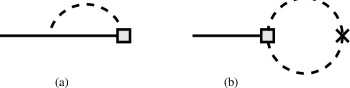
Figure 4: Corrections to the weak current vertex. The box represents an insertion of the weak current.

It is easy to see that the diagram Fig. 4a vanishes: the loop integral must be proportional to $v^{\mu}$, which will vanish when contracted with the projection operator in the numerator of the $B^{*}$ propagator. The remaining tadpole graph Fig. 4b yields

$${{\rm i}\alpha v^{\mu}\over 2}{(-2\alpha_{0}M_{d}^{2}+m_{0}^{2})/3\over 16\pi^{2}f^{2}}\log({M_{d}^{2}\over\mu^{2}}).$$ (36)

The final results for the decay constants are then found by combining the wavefunction and vertex corrections:

$$\sqrt{M_{B}}f_{B}=\alpha\left[1-{1\over 2}(1+3g^{2})\,\mu_{q}-(3g\gamma-(1+3g^{2}){\alpha_{0}\over 3})\,\mu_{d}+\kappa_{1}m_{d}\right].$$ (37)

In contrast, the results in the full theory are[10, 11]

$$\sqrt{M_{B_{d}}}f_{B_{d}} = \alpha\left[1-{1\over 2}(1+3g^{2})\left({3\over 2}\,\mu_{\pi}+\,\mu_{K}+{1\over 6}\,\mu_{\eta}\right)+\kappa_{1}m_{d}+\kappa_{2}(m_{s}+2m_{d})\right],$$

$$\sqrt{M_{B_{s}}}f_{B_{s}} = \alpha\left[1-{1\over 2}(1+3g^{2})\left(2\,\mu_{K}+{2\over 3}\,\mu_{\eta}\right)+\kappa_{1}m_{s}+\kappa_{2}(m_{s}+2m_{d})\right].$$ (38)

3.3 Masses

The correction to the mass is obtained by evaluating the self-energy on-shell and removing the wavefunction renormalization constant (though to the order I am working it does not contribute). Defining

$$M_{B}=\overline{M}_{B}-{3\over 4}\Delta+\delta M_{B}$$ (39)

where $\overline{M}_{B}$ is the spin-averaged mass in the chiral limit, $\Delta$ is the hyperfine splitting and $\delta M_{B}$ is the light-quark dependent contribution to the mass, I find

$$\delta M_{B^{0}}=2\lambda_{1}\,m_{d}-{2\pi\over 16\pi^{2}f^{2}}\left(g^{2}\,{m_{0}^{2}\over 3}M_{d}+(2g\gamma-5g^{2}{\alpha_{0}\over 3})M_{d}^{3}\right).$$ (40)

while in the unquenched theory[11, 12]

$$\delta M_{B_{s}}-\delta M_{B_{d}}=2\lambda_{1}(m_{s}-m_{d})-{\pi g^{2}\over 16\pi^{2}f^{2}}(-3m_{\pi}^{3}+2m_{K}^{3}+m_{\eta}^{3}).$$ (41)

3.4 Mixing

The constant $B_{B_{a}}$ is defined as the ratio

$$B_{B_{a}}={\langle\overline{B}_{a}|\overline{q}_{L}^{a}\gamma_{\mu}b_{L}\,\overline{q}_{L}^{a}\gamma^{\mu}b_{L}|B_{q}\rangle\over{8\over 3}\langle\overline{B}_{a}|\overline{q}_{L}^{a}\gamma_{\mu}b_{L}|0\rangle\langle 0|\overline{q}_{L}^{a}\gamma^{\mu}b_{L}|B_{a}\rangle}={\langle\overline{B}_{a}|\overline{q}_{L}^{a}\gamma_{\mu}b_{L}\,\overline{q}_{L}^{a}\gamma^{\mu}b_{L}|B_{q}\rangle\over{2\over 3}f_{B_{a}}^{2}m_{B_{a}}^{2}\,B_{B_{a}}}.$$ (42)

As shown by Grinstein and collaborators[10], in the effective theory the operator

$$\overline{q}_{L}^{a}\gamma_{\mu}b_{L}\,\overline{q}_{L}^{a}\gamma^{\mu}b_{L}$$ (43)

is represented by

$$4\beta\mathop{\rm tr}_{D}\nolimits\left[(\xi\overline{H}^{(b)})^{a}\gamma_{\mu}L\right]\mathop{\rm tr}_{D}\nolimits\left[(\xi H^{(\overline{b})})^{a}\gamma^{\mu}L\right],$$ (44)

which is essentially just the square of the left-handed current. The one-loop corrections to this operator are shown in Fig. (6).

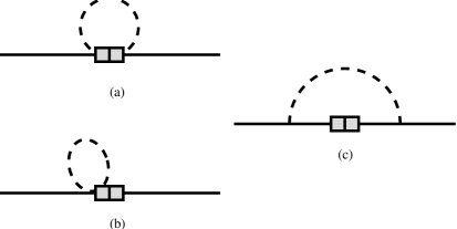
Figure 6: The corrections to $B-\overline{B}$ mixing. The double box represents an insertion of the mixing operator. Corresponding diagrams with hairpin vertices are not shown.

There are two types of tadpoles which arise from the operator Eq. (43): those where each $\xi$ is expanded to $O(\phi)$ (Fig. 6a) and those where only one of the $\xi$’s is expanded (Fig. 6b). The latter tadpoles just renormalize $f_{B}$ and will cancel in the ratio for $B_{B}$. Thus it is only necessary to consider the former. I find

$$B_{B_{d}}=4\beta\left[1-(1-3g^{2})\left((1-{2\over 3}\alpha_{0})\,\mu_{d}+\,\mu_{q}\right)+6g\gamma\,\mu_{d}+\beta_{1}m_{d}\right],$$ (45)

which should be compared with the unquenched results[10] ($\beta_{1}$ and $\beta_{2}$ are additional counter-terms)

$$B_{B} = 4\beta\left[1-(1-3g^{2}){2\over 3}\,\mu_{\eta}+\beta_{1}m_{d}+\beta_{2}(m_{s}+2m_{d})\right],$$ (46)

$$B_{B_{s}} = 4\beta\left[1-(1-3g^{2})\left({1\over 2}\,\mu_{\pi}+{1\over 6}\,\mu_{\eta}\right)+\beta_{1}m_{s}+\beta_{2}(m_{s}+2m_{d})\right].$$ (47)

The reader will note that in contrast to the earlier results, $B_{B}$ has true chiral logarithms even in the absence of the singlet coupling $\gamma$ and the kinetic coupling $\alpha_{0}$. A similar phenomenon occurs in $B_{K}$, as shown by Sharpe[3]. The reason is that flavor conservation allows disconnected quark loops to appear only in the guise of the $\eta^{\prime}$, so that even in full QCD they do not contribute.

3.5 Isgur-Wise Function

The heavy quark current which mediates the decay $B\rightarrow De\nu$ is represented at leading order by

$$\xi_{0}(w)\mathop{\rm tr}_{D}\nolimits[\overline{H}_{a}^{(c)}(v^{\prime})\gamma_{\mu}LH_{a}^{(b)}(v)],$$ (48)

where $\xi_{0}(w)$ ($w=v\cdot v^{\prime}$) is the leading-order Isgur-Wise function. In the full theory, the leading corrections are[11, 13] (here the counter-terms $\eta_{1}$ and $\eta_{2}$ are functions of $w$)

$$\xi_{u,d} = \xi_{0}(w)\left[1+2g^{2}(r(w)-1)\left({3\over 2}\,\mu_{\pi}+\,\mu_{K}+{1\over 6}\,\mu_{\eta}\right)\right.$$

$$\phantom{\xi_{0}(w)}+\left.2(r(w)-1)\biggl{(}\eta_{1}(w)m_{d}+\eta_{2}(w)(m_{s}+2m_{d})\biggr{)}\right],$$

$$\xi_{s} = \xi_{0}(w)\left[1+2g^{2}(r(w)-1)\left(2\,\mu_{K}+{2\over 3}\,\mu_{\eta}\right)\right.$$ (49)

$$\phantom{\xi_{0}(w)}+\left.2(r(w)-1)\biggl{(}\eta_{1}(w)m_{s}+\eta_{2}(w)(m_{s}+2m_{d})\biggr{)}\right],$$

where

$$r(w)={1\over\sqrt{w^{2}-1}}\log(w^{2}+\sqrt{w^{2}-1}).$$ (50)

The quenched results take the by-now-expected form

$$\xi_{d}(w)=\xi_{0}(w)\left[1+2(r(w)-1)\left(g^{2}\,\mu_{q}+(2g\gamma-{2\over 3}g^{2}\alpha_{0})\,\mu_{d}+\eta_{1}(w)m_{d}\right)\right].$$ (51)

4 Discussion and Numeric Results

To obtain numeric values it is necessary to know the values of the various couplings which enter the Lagrangian. Combining data on the $D^{*}$ width and branching fractions[14, 15], Amundson et al. Ref. ([]Amundson:g) obtained the constraint $0.1<g^{2}<0.5$. The spread is caused by the uncertainty in the branching fraction $BR(D^{*+}\rightarrow D^{+}\gamma)$; taking the central value yields $g\simeq 0.5$. QCD sum rules[17] and relativistic quark models[18] favor a smaller value, $g\sim 1/3$. Given this uncertainty, I will show results for different values of the coupling. There is no information on the coupling $\gamma$, but $1/N_{c}$ arguments suggest that it is small. They also suggest that $\alpha_{0}$ is small; direct evidence from $\eta-\eta^{\prime}$ mixing confirms this. Consequently, I will take both $\gamma$ and $\alpha_{0}$ to vanish. The maximum value of $w$ in the decay $B\rightarrow Dl\nu$ is about $1.8$, so I will use $r(1.8)=0.76$ when evaluating $\xi$. Finally, I will choose $\mu=1{\rm\,GeV}$.

There are several ways to determine $m_{0}$, each giving a different result. The Witten-Veneziano large $N_{c}$ formula[20] $m_{0}^{2}=m_{\eta^{\prime}}^{2}+m_{\eta}^{2}-2m_{K}^{2}$ gives $m_{0}\approx 852{\rm\,MeV}$, while from the $\eta-\eta^{\prime}$ mass splitting Sharpe[3] estimated $m_{0}\approx 900{\rm\,MeV}$. It has also been computed directly on the lattice. Early attempts[21] found $m_{0}\approx 570-920{\rm\,MeV}$, but with limited statistics and a strong dependence on the lattice spacing. Recently, a more accurate computation has been performed. Kuramashi et al.[22] extracted $m_{0}$ by comparing the one and two loop contributions to the $\eta^{\prime}$ propagator; they found $m_{0}=751(39){\rm\,MeV}$. Using the $U(1)$ Ward identity relation $m_{0}^{2}=6\chi/f_{\pi}^{2}$, with $\chi$ the topological susceptibility, the same group found $m_{0}=1146(67)$ with $\chi$ and $f_{\pi}$ obtained on the same lattice. They attributed this larger result to contamination from extra terms in the Ward identity induced by the use of Wilson fermions. I will choose $m_{0}=750{\rm\,MeV}$, but will also show some results for $m_{0}=1100{\rm\,MeV}$.

For an honest calculation, it is also necessary to specify the $O(m_{q})$ counter-terms. But it is an unfortunate fact that there is little to constrain them, save the general expectation that their natural scale is $\Lambda_{\chi}\approx 4\pi f$. A common practice when confronted with this situation to assume that the counter-terms are overshadowed by the logarithmic contributions. Another approach is to reduce the dependence on these unknown terms by taking appropriate ratios. Fortunately, since it is expected that the coefficients in the chiral expansion should be (almost) the same in the quenched and full theories, some of the counter-terms will cancel when the predictions of the two theories are subtracted to compute the error. In particular, the errors in $f_{B_{s}}/f_{B_{d}}$, $\xi_{s}/\xi_{d}$, $B_{B_{s}}/B_{B_{d}}$ and $\delta M_{B_{s}}-\delta M_{B_{d}}$ are free of counter-terms. Results for these quantities are shown in Table 2; in order to illustrate the $m_{0}$ dependence, the quenched results are shown at both $m_{0}=750{\rm\,MeV}$ and $m_{0}=1100{\rm\,MeV}$.

Table 2: Quenched and full heavy-light quantities. Only the non-analytic part of the mass difference is shown.

Quantity	Unquenched	$m_{0}=750{\rm\,MeV}$	$m_{0}=1100{\rm\,MeV}$
$f_{B_{s}}/f_{B_{d}}-1$	$0.074(1+3g^{2})$	$-0.11(1+3g^{2})$	$-0.23(1+3g^{2})$
$B_{B_{s}}/B_{B_{d}}-1$	$0.052(1-3g^{2})$	$-0.11(1-3g^{2})$	$-0.36(1-3g^{2})$
$\xi_{s}/\xi_{d}-1$	$0.059\,g^{2}$	$-0.086\,g^{2}$	$-0.18\,g^{2}$
$\delta M_{B_{s}}-\delta M_{B_{d}}$	$-450\,g^{2}{\rm\,MeV}$	$-340\,g^{2}{\rm\,MeV}$	$-740\,g^{2}{\rm\,MeV}$

The ratios in the quenched theory are computed by substituting $M_{s}=\sqrt{2m_{K}^{2}-m_{\pi}^{2}}=680{\rm\,MeV}$ and $M_{d}=m_{\pi}$. Concentrating on the results at $m_{0}=750{\rm\,MeV}$, one sees that the corrections to the ratios are similar in magnitude but opposite in sign to those in the full theory. This is a result of the fact that the quenched logarithms diverge in the chiral limit. Notice that the corrections for the mass splittings threaten to be larger than the splittings themselves unless $g$ is small. This suggests either a large cancelation occurs with the leading $\lambda_{1}$ term or higher-order corrections are important. Either solution casts doubt on the reliability of the error estimates in this case.

While the results in Table 2 suggest large quenching errors — particularly in $f_{B_{s}}/f_{B}$ — it is likely that the error in actual simulations will be less. The reason is the following. Currently, most simulations are performed with quark masses corresponding to pion masses in the range $400\mathrel{\mathchoice{\lower 3.0pt\vbox{\halign{$\m@th\displaystyle\hfill#\hfil$\cr<\crcr\sim\crcr}}}{\lower 3.0pt\vbox{\halign{$\m@th\textstyle\hfill#\hfil$\cr<\crcr\sim\crcr}}}{\lower 3.0pt\vbox{\halign{$\m@th\scriptstyle\hfill#\hfil$\cr<\crcr\sim\crcr}}}{\lower 3.0pt\vbox{\halign{$\m@th\scriptscriptstyle\hfill#\hfil$\cr<\crcr\sim\crcr}}}}M_{\pi}\mathrel{\mathchoice{\lower 3.0pt\vbox{\halign{$\m@th\displaystyle\hfill#\hfil$\cr<\crcr\sim\crcr}}}{\lower 3.0pt\vbox{\halign{$\m@th\textstyle\hfill#\hfil$\cr<\crcr\sim\crcr}}}{\lower 3.0pt\vbox{\halign{$\m@th\scriptstyle\hfill#\hfil$\cr<\crcr\sim\crcr}}}{\lower 3.0pt\vbox{\halign{$\m@th\scriptscriptstyle\hfill#\hfil$\cr<\crcr\sim\crcr}}}}1000{\rm\,MeV}$. The results are then extrapolated linearly (in the quark mass) to the chiral limit and the physical $m_{\pi}$. Due to the familiar property of the logarithm, quenched loop corrections change as much in the interval $140<M_{d}<350{\rm\,MeV}$ as they do in the interval $350<M_{d}<1000{\rm\,MeV}$. Consequently, in the mass range covered by lattice simulations the quenched logarithm appears linear. This can be seen in Fig. 8, where both the “true” quenched and linearly extrapolated predictions for $f_{B}$ are shown.

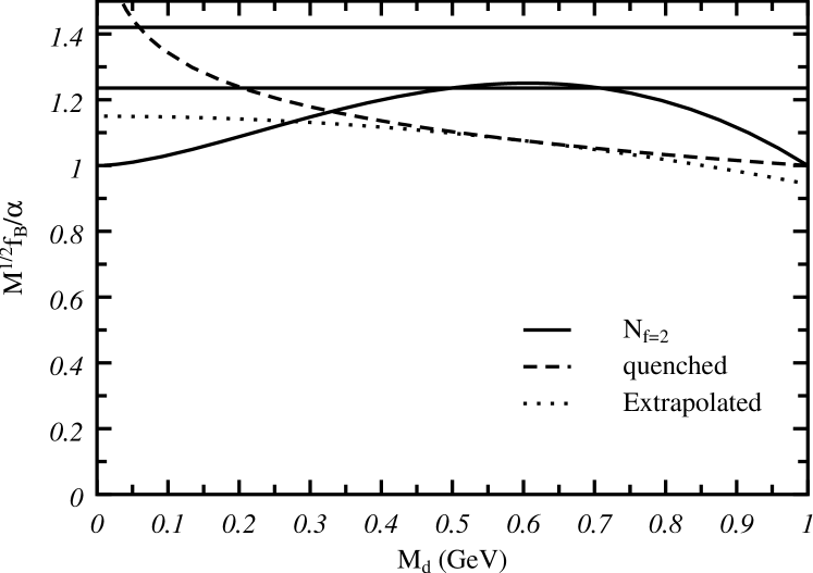
Figure 8: Quenched and unquenched corrections to $f_{B}$ as a function of meson mass. Also shown is a linear (in the quark, not the meson mass) extrapolation of the quenched $f_{B}$. The horizontal lines are the predictions for $f_{B_{s}}$ and $f_{B}$ in the full theory.

Clearly, the two cannot be distinguished for masses greater than say $300{\rm\,MeV}$, but the extrapolated result underestimates the “true” behavior by more than $10\%$ at $M_{d}=m_{\pi}$. While the primary motivation for this extrapolation is the desire to efficiently invert the quark propagators, it has the side-effect of reducing the quenching errors. Moreover, it is the correct thing to do, since the goal is to describe unquenched QCD and quenched ChPT clearly fails to do this in the chiral limit. Table 4 compares the two methods of computing the error at different values of the coupling.

Table 4: The errors for different choices of the coupling $g$. Results are shown using both the exact and extrapolated quenched predictions. An error is negative when the quenched quantity is smaller than the full.

Errors	Exact			Extrapolated
	$g=0.7$	0.5	0.33	0.7	0.5	0.33
$f_{B_{s}}/f_{B_{d}}$	$-0.45$	$-0.32$	$-0.24$	$-0.28$	$-0.20$	$-0.15$
$B_{B_{s}}/B_{B_{d}}$	$0.078$	$-0.041$	$-0.11$	$0.012$	$-0.0062$	$-0.017$
$\xi_{s}/\xi_{d}$	$-0.072$	$-0.036$	$-0.016$	$-0.045$	$-0.023$	$-0.010$
$M_{B_{s}}-M_{B_{d}}$	$49{\rm\,MeV}$	$25{\rm\,MeV}$	$11{\rm\,MeV}$	-	-	-

One sees that the error is substantially reduced by the extrapolation. The errors in $B_{B}$ and $\xi$ are relatively small to start with and become negligible when extrapolated. However, even with the extrapolation the error in $f_{B}$ is larger then one might have hoped. Note also that $f_{B_{s}}/f_{B}$ is smaller in the quenched theory.

In fact, the size of the error in $f_{B}$ is easy to understand. For the Isgur-Wise function, the error is small because the corrections themselves are small. Conversely, the corrections to $f_{B}$ are large and so the error is large. Moreover, they are driven by the tadpole terms, which remain large even if the coupling $g$ vanishes. The tadpoles, however, do not depend on the heavy quark mass, so it should be possible to eliminate them by studying the $1/M$ corrections[23].

Some additional understanding of the differences between the quenched and dynamical theories may be gained by comparing them in the mass range probed on the lattice. For this it may be better to consider a two quark theory with degenerate masses (rather than the full three-flavor theory), since it is closer to the type of theory studied in unquenched simulations. In Fig. 8 the predictions for $f_{B}$ are shown. Here I have neglected the unknown counter-terms, though it is clear from the graph that there must be a positive term of $O(m_{d})$ since lattice simulations find that $f_{B}$ increases with the light quark mass. There are two general features that should be noted in Fig. 8. First, that in both the quenched and two-flavor theories, $f_{B}$ is less than both $f_{B_{d}}$ and $f_{B_{s}}$. This may be attributed to the fact that the full theory has more mesons contributing to loop corrections. The second observation is that the gap between the two-flavor and quenched corrections grows as $M_{d}$ increases toward the point $M_{s}=\sqrt{2m_{K}^{2}-m_{\pi}^{2}}$. Thus, the fact that quenching decreases the ratio $f_{B_{s}}/f_{B_{d}}$ is due to the different nature of the quenched logarithm. Finally, Table 6 compares the quenched and two-flavor predictions at a representative mass of $M_{d}=600{\rm\,MeV}$ (again neglecting counter-terms).

Table 6: Quenched and unquenched results at $M_{d}\,(=m_{\pi})=600{\rm\,MeV}$.

Quantity	$m_{0}=750{\rm\,MeV}$	Unquenched ($N_{f}=2$)
$\sqrt{M}f_{B}/\alpha-1$	$0.031(1+3g^{2})$	$0.10(1+3g^{2})$
$B_{B}/4\beta-1$	$0.20(1-3g^{2})$	$0.069(1-3g^{2})$
$\xi_{d}/\xi_{0}-1$	$0.025\,g^{2}$	$0.083\,g^{2}$

It can be seen that the errors are comparable to those found in the extrapolated ratios.

5 Conclusions

I have included heavy mesons into the framework of quenched chiral perturbation theory and used it to study the error arising from the use of the quenched approximation in lattice studies of heavy-light mesons. These lattice studies are important for the phenomenology of the standard model. Because estimates of the error depend on the as-yet unmeasured value of the the $B^{*}B\pi$ coupling $g$, results were shown for several values of $g$ in the allowed range. It was seen that the errors in $B_{B}$ and $\xi(w)$ were negligible. However, the error in $f_{B}$ was surprisingly large, more than $15\%$ in the best case. It was observed that the large error follows from the large corrections present in both theories. These large corrections were traced to the tadpole corrections, and it was suggested that they might be eliminated by studying the $1/M$ corrections to the theory. Indeed, Grinstein[24, 9] has advocated doing just that in the continuum by studying the double ratio ${f_{B_{s}}/f_{B}\over f_{D_{s}}/f_{D}}$. This is done for the quenched theory in a forthcoming work[23].

A general conclusion that can be drawn from the quenched chiral calculation is that quenching tends to decrease the ratio $f_{D_{s}}/f_{D}$. This is in agreement with the one unquenched simulation[1], which found $f_{D_{s}}/f_{D}=1.34$, a value larger than that typically found in quenched calculations. This may have implications for reconciling lattice predictions of $f_{D_{s}}$ with the recent CLEO measurement[25].

In the future it would be interesting to study heavy baryons containing two light quarks within this framework. Because of the presence of two light quarks, the quenched theory will be less trivial and the loop corrections will have a more complicated flavor structure, more closely resembling that of the light mesons. It would also be useful to to move beyond $1/N_{c}$ arguments for the magnitude of $\gamma$. It appears that it could be calculated within QCD sum rules using the same techniques that have recently been applied to $g$[17].

A Renormalization Constants

Within the context of dimensional regularization, the singularities of the effective Lagrangian are customarily described in terms of the parameter $L(\mu)$ which contains the singularity at $D=4$ (recall $D=4-2\epsilon$, $1/\hat{\epsilon}=1/\epsilon+\log 4\pi-\gamma_{\rm E}+1$):

$$L(\mu)={1\over 16\pi^{2}}\mu^{-2\epsilon}{1\over\hat{\epsilon}}.$$ (A.1)

It is convenient to decompose an arbitrary coupling $k$ as $k=k^{\rm r}(\mu)+\overline{k}\,L(\mu)$.

To render the Lagrangian Eq. (27) finite, it is necessary to add the counter-term

$$3\,g^{2}{m_{0}^{2}\over f^{2}}\mathop{\rm tr}_{D}\nolimits\left[\overline{H}_{a}iv\cdot D_{ba}H_{b}\right]\,L(\mu).$$ (A.2)

In addition, $\overline{k}_{1}$ must be taken to be

$$\overline{k}_{1}=6(g\gamma-{1\over 3}\,g^{2}\alpha_{0}){2\mu_{0}\over f^{2}}.$$ (A.3)

The current Eq. (28) is renormalized with

$$\overline{\kappa}_{1}=-((1+3g^{2})\frac{\alpha_{0}}{3}-3g\gamma)\,{2\mu_{0}\over f^{2}}.$$ (A.4)

and in addition $\alpha$ must be rescaled:

$$\alpha^{\rm r}(\mu)=\alpha\left[1+{1\over 2}(1+3g^{2}){m_{0}^{2}/3\over f}\,L(\mu)\right].$$ (A.5)

The description of $B-\overline{B}$ mixing requires the counter-term (no sum on $a$)

$$4\,\beta\,\beta_{1}\mathop{\rm tr}_{D}\nolimits\left[(\xi\overline{H}^{(b)})^{a}\gamma_{\mu}L\right]\mathop{\rm tr}_{D}\nolimits\left[(\xi H^{(\overline{b})})^{a}\gamma^{\mu}L\right]({\cal M}_{+})_{aa},$$ (A.6)

and the couplings must be

$$\beta^{\rm r}(\mu) = \beta\left(1+(1-3g^{2}){m_{0}^{2}/3\over f}L(\mu)\right),$$ (A.7)

$$\overline{\beta}_{1} = \left((1-3g^{2})(1-{2\over 3}\alpha_{0})-6g\gamma\right){2\mu_{0}\over f^{2}}.$$ (A.8)

Finally, the Lagrangian for $b\rightarrow c$ transitions needs the counter-term

$$\eta(w)(r(w)-1)\mathop{\rm tr}_{D}\nolimits[\overline{H}_{a}^{(c)}(v^{\prime})\gamma_{\mu}LH_{b}^{(b)}(v)]({\cal M}_{+})_{ba},$$ (A.9)

with

$$\overline{\eta}(w)=-4(g\gamma-{1\over 3}g^{2}\alpha_{0})\,{2\mu_{0}\over f^{2}}$$ (A.10)

and the rescaled coupling

$$\xi_{0}^{\rm r}(w,\mu)=\xi_{0}(w)\left(1+2(r(w)-1)\,g^{2}{m_{0}^{2}/3\over 3}L(\mu)\right).\\$$ (A.11)

References

• [1] K. M. Bitar, et al. Phys. Rev. D 49, 3546 (1994).
• [2] A. Morel, J. Physique 48, 111 (1987).
• [3] S. R. Sharpe, Phys. Rev. D 46, 3146 (1992).
• [4] C. W. Bernard and M. F. L. Golterman, Phys. Rev. D 46, 853 (1992);
Nucl. Phys. B (Proc. Suppl.) 26, 360 (1992).
• [5] J. N. Labrenz and S. R. Sharpe, preprint UW-PT-93-07 (hep-lat/9312067), to be published in the proceedings of the International Symposium on Lattice Field Theory, Dallas, Texas, 1993.
• [6] M. Wise, Phys. Rev. D 45, 1992 (2188); G. Burdman and J. F. Donoghue, Phys. Lett. B 280, 287 (1992); T. M. Yan et al., Phys. Rev. D 46, 1148 (1992).
• [7] C. W. Bernard and M. F. L. Golterman, Nucl. Phys. B(Proc. Suppl.) 30 (1993) 217.
• [8] S. R. Sharpe, Nucl. Phys. B (Proc. Suppl.) 30, 213 (1993).
• [9] C. G. Boyd and B. Grinstein, UCSD/PTH 93-46 (hep-th/9402340).
• [10] B. Grinstein et al., Nucl. Phys. B 380, 369 (1992).
• [11] J. Goity, Phys. Rev. D 46, 3929 (1992).
• [12] E. Jenkins, Nucl. Phys. B 412, 181 (1994).
• [13] E. Jenkins and M. Savage, Phys. Lett. B 281, 331 (1992).
• [14] S. Barlag et al. (ACCMOR Collaboration), Phys. Lett. B 278, 480 (1992).
• [15] F. Butler et al.(CLEO Collaboration), Phys. Rev. Lett. 69, 2041 (1992).
• [16] J. Amundson, et al., Phys. Lett. B 296, 415 (1992); S. Stone, Heavy Flavors, A. Buras and H. Lindner, eds., World Scientific, Singapore (1992).
• [17] V. M. Belyaev et al., preprint MPI-PhT/94-62 (hep-ph/9410280); P. Colangelo et al., preprint UGVA-DPT 1994/06-856 (hep-ph/9406295); A. Grozin and O. I. Yakovlev, preprint BUDKERINP-94-3 (hep-ph/9401267); V. L. Eletsky and Ya. I. Kogan, Z. Phys. C 28, 155 (1985).
• [18] P. Colangelo, F. D. Fazio, and G. Nardulli, Phys. Lett. B 334, 175 (1994); M. Sutherland, B. Holdom, S. Jaimungal, and R. Lewis, preprint UTPT-94-25 (hep-ph/9410324).
• [19] T. Hatsuda, Nucl. Phys. B 329, 376 (1990).
• [20] E. Witten, Nucl. Phys. B 156, 269 (1979); G. Veneziano, Nucl. Phys. B 159, 213 (1979).
• [21] M. Fukugita, T. Kaneko and A. Ukawa, Phys. Lett. B 145, 93 (1984); S. Itoh, Y. Iwasaki and T. Yoshié, Phys. Rev. D 36, 527 (1987).
• [22] Y. Kuramashi et al., Phys. Rev. Lett. 72, 3448 (1994) and also Y. Kuramashi et al., preprint KEK-CP-010 (hep-lat/9312016), to be published in the proceedings of the International Symposium on Lattice Field Theory, Dallas, Texas, 1993.
• [23] M. J. Booth, preprint IFT-94-10.
• [24] B. Grinstein, Phys. Rev. Lett. 71, 3067 (1993).
• [25] D. Accosta et al. (CLEO Collaboration), Phys. Rev. D 49, 5690 (1994).