Semileptonic tau decays, structure functions, kinematics and polarisation

The most general angular distribution of two or three meson final states from semileptonic decays $\tau\rightarrow\pi\pi\nu$, $K\pi\nu$, $\pi\pi\pi\nu$, $K\pi\pi\nu$, $K\pi\nu$, $KKK\nu$, $\eta\pi\pi\nu,\,\ldots{}$ of polarized $\tau$ leptons can be characterized by 16 structure functions. Predictions for hadronic matrix elements, based on CVC and chiral Lagrangians and their relations to the structure functions are discussed. Most of them can be determined in currently ongoing high statistics experiments. Emphasis of the kinematical analysis is firstly put on $\tau$ decays in $e^{+}e^{-}$ experiments where the neutrino escapes detection and the $\tau$ rest frame cannot be reconstructed. Subsequently it is shown, how the determination of hadron tracks in double semileptonic events allows to fully reconstruct the $\tau$ kinematics. The implications for the spin analysis are indicated.

1 Structure functions

$\tau$-decays provide an ideal for studying strong interaction physics and resonance properties. Detailed information on the hadronic charged current for the decay into three pseudoscalar mesons can be derived in particular from the study of angular distributions. Consider the semileptonic $\tau$-decay

$$\tau(l,s)\rightarrow\nu(l^{\prime},s^{\prime})+h_{1}+h_{2}+h_{3}\>,$$ (1)

into the pseudoscalar mesons $h_{i}(q_{i},m_{i})$ and which is governed by the matrix element

$${\cal{M}}=\frac{G}{\sqrt{2}}\,\bigl{(}^{\cos\theta_{c}}_{\sin\theta_{c}}\bigr{)}\,M_{\mu}J^{\mu}\>,$$ (2)

with $G$ the Fermi-coupling constant. The cosine and the sine of the Cabbibo angle ($\theta_{C}$) in (2) enter for Cabibbo allowed $\Delta S=0$ and Cabibbo suppressed $|\Delta S|=1$ decays, respectively. The leptonic ($M_{\mu}$) and hadronic ($J^{\mu}$) currents are given by

$$M_{\mu}=\bar{u}(l^{\prime},s^{\prime})\gamma_{\mu}(g_{V}-g_{A}\gamma_{5})u(l,s)$$ (3)

and

$$J^{\mu}(q_{1},q_{2},q_{3})=\langle h_{1}h_{2}h_{3}|V^{\mu}(0)-A^{\mu}(0)|0\rangle.$$ (4)

$V^{\mu}$ and $A^{\mu}$ are the vector and axialvector quark currents, respectively. The most general ansatz for the matrix element of the quark current $J^{\mu}$ is characterized by four formfactors [1]

$$J^{\mu}=V_{1}^{\mu}\,F_{1}+V_{2}^{\mu}\,F_{2}+\,i\,V_{3}^{\mu}\,F_{3}+V_{4}^{\mu}\,F_{4}\>,$$ (5)

with

$$\begin{array}[]{ll}V_{1}^{\mu}&=q_{1}^{\mu}-q_{3}^{\mu}-Q^{\mu}\frac{Q(q_{1}-q_{3})}{Q^{2}}\>,\\[5.69054pt] V_{2}^{\mu}&=q_{2}^{\mu}-q_{3}^{\mu}-Q^{\mu}\frac{Q(q_{2}-q_{3})}{Q^{2}}\>,\\[5.69054pt] V_{3}^{\mu}&=\epsilon^{\mu\alpha\beta\gamma}q_{1\,\alpha}q_{2\,\beta}\>q_{3\,\gamma}\\[5.69054pt] V_{4}^{\mu}&=q_{1}^{\mu}+q_{2}^{\mu}+q_{3}^{\mu}\,=Q^{\mu}\>.\end{array}$$ (6)

The formfactors $F_{1}$ and $F_{2}$ ($F_{3}$) originate from the axial vector hadronic current (vector current) and lead to spin 1 states, whereas $F_{4}$ is due to the spin zero part of the axial current matrix element. The formfactors $F_{1}$ and $F_{2}$ can be predicted by chiral Lagrangians, supplemented by informations about resonance parameters. Parametrizations of the amplitude for the $3\pi$ final states can be found in [1, 2, 3]. In this case the axial formfactors $F_{3}$ is absent due to the $G$ parity of the pions. (The isospin violating transition $\tau\to\nu\pi\omega(\to\pi\pi)$ would, however, give rise to such terms. See [4]) The formfactor $F_{4}$ is assumed to be absent as a consequence of PCAC, an assumption to be tested experimentally. The $2\pi$ and $3\pi$ decay modes offer a unique tool for the study of $\rho,\rho^{\prime}$ resonance parameters in diffent hadronic enviroments, competing well with low enery $e^{+}e^{-}$ colliders with energies in the region below 1.7 GeV. As we will see later, the two body ($\rho$ and $\rho^{\prime}$) resonance parameters can be determined in the $3\pi$ mode by taking ratios of hadronic structure functions, whereas the measurement of four structure functions can be used to put constraints on the $a_{1}$ parameters. The decay modes involving different mesons (for example $K\pi\pi,\,KK\pi$ or $\eta\pi\pi$) allow for axial and vector current contributions at the same time. Explicit parametrizations for the form factors in these decay modes are presented in [5, 6, 7]. The vector formfactor $F_{3}$ is related to the Wess-Zumino anomaly [8], whereas the axial vector form factors are again predicted by chiral lagrangians. The latter decay modes allow also for the study of $J^{PC}=0^{-+}$ and $J^{PC}=1^{++}$ resonances which are not directly accessible in electron positron annihilation.

Let us now introduce the formalism of the hadronic structure functions. The differential decay rate is obtained from

$$d\Gamma(\tau\rightarrow\nu_{\tau}\,3h)=\frac{G^{2}}{4m_{\tau}}\,\bigl{(}^{\cos^{2}\theta_{c}}_{\sin^{2}\theta_{c}}\bigr{)}\,L_{\mu\nu}H^{\mu\nu}\,d\mbox{PS}$$

where $L_{\mu\nu}=M_{\mu}(M_{\nu})^{\dagger}$ and $H^{\mu\nu}\equiv J^{\mu}(J^{\nu})^{\dagger}$. The decays are most easily analyzed in the hadronic rest frame where $\vec{q}_{1}+\vec{q}_{2}+\vec{q}_{3}=\vec{Q}=0$. The orientation of the hadronic system is characterized by three Euler angles ($\alpha,\beta$ and $\gamma$) as introduced in [1, 3]. In the hadronic rest frame the product of the hadronic and the leptonic tensors reduces to the following sum [1]

$$L^{\mu\nu}H_{\mu\nu}=\sum_{X}L_{X}W_{X}.$$ (7)

In this system the hadronic tensor $H^{\mu\nu}$ is decomposed into 16 (real) hadronic structure functions $W_{X}$ corresponding to 16 density matrix elements for a hadronic system in a spin one [$V_{1}^{\mu},V_{2}^{\mu},V_{3}^{\mu}$] and spin zero state $[V_{4}^{\mu}]$ (nine of them originate from a pure spin one, one from a pure spin zero and six from interference terms). The 16 structure functions describe the dynamics of the three meson decay and depend only on $Q^{2}$ and the Dalitz plot variables $s_{i}$. The factors $L_{X}$ depend on the Euler angles (which determine the orientation of the hadronic system), on the $\tau$ polarization, on the chirality parameter $\gamma_{VA}$ of the $\tau\nu W$-vertex and on the total energy of the hadrons in the laboratory frame. This latter dependence disappears if one considers the $\tau$ decay in its restframe where it is replaced by the emission angle of the hadron relative to the $\tau$ spin. Analytical expressions for the 16 coefficients $L_{X}$ were first presented in [1]. The formalism can be applied to the case, where the $\tau$ rest frame cannot be reconstructed because of the unknown neutrino momentum and to the case discussed below, where the full kinematic information is available. The dependence of the coefficients $L_{X}$ on the $\tau$ polarization allows for an improved measurement of the $\tau$ polarization at LEP [see for example [9, 10, 11] and references therein].

Figure 1: Ratio of the spin one hadronic structure functions $w_{C}/w_{A},w_{D}/w_{A},w_{E}/w_{A}$ (from top to bottom) for $\tau\rightarrow\nu\pi\pi\pi$ as a function of $Q^{2}$.

The hadronic structure functions $W_{X}$ on the other hand contain the full dynamics of the hadronic decay. The measurement of these structure functions provides a unique tool for low enery hadronic physics. They can be calculated from the components of the hadronic current $J^{\mu}$ and expressed in terms of the form factors $F_{i}$. For brevity only the results for the pure spin one state are listed.

$$\hskip 8.53581ptW_{A} = \hskip 8.53581pt(x_{1}^{2}+x_{3}^{2})\,|F_{1}|^{2}+(x_{2}^{2}+x_{3}^{2})\,|F_{2}|^{2}$$

$$~{}~{}+2(x_{1}x_{2}-x_{3}^{2})\mbox{Re}\left(F_{1}F^{\ast}_{2}\right)\>,$$

$$W_{B} = \hskip 8.53581ptx_{4}^{2}|F_{3}|^{2}$$

$$W_{C} = \hskip 8.53581pt(x_{1}^{2}-x_{3}^{2})\,|F_{1}|^{2}+(x_{2}^{2}-x_{3}^{2})\,|F_{2}|^{2}$$

$$~{}~{}+2(x_{1}x_{2}+x_{3}^{2})\mbox{Re}\left(F_{1}F^{\ast}_{2}\right)$$

$$W_{D} = \hskip 8.53581pt2[x_{1}x_{3}\,|F_{1}|^{2}-x_{2}x_{3}\,|F_{2}|^{2}$$

$$~{}~{}+x_{3}(x_{2}-x_{1})\mbox{Re}(F_{1}F^{\ast}_{2})]$$

$$W_{E} = -2x_{3}(x_{1}+x_{2})\,\mbox{Im}\left(F_{1}F^{\ast}_{2}\right)$$ (8)

$$W_{F} = \hskip 8.53581pt2x_{4}\left[x_{1}\,\mbox{Im}\left(F_{1}F^{\ast}_{3}\right)+x_{2}\,\mbox{Im}\left(F_{2}F^{\ast}_{3}\right)\right]$$

$$W_{G} = -2x_{4}\left[x_{1}\,\mbox{Re}\left(F_{1}F^{\ast}_{3}\right)+x_{2}\,\mbox{Re}\left(F_{2}F^{\ast}_{3}\right)\right]]$$

$$W_{H} = \hskip 8.53581pt2x_{3}x_{4}\left[\,\mbox{Im}\left(F_{1}F^{\ast}_{3}\right)-\,\mbox{Im}\left(F_{2}F^{\ast}_{3}\right)\right]$$

$$W_{I} = -2x_{3}x_{4}\left[\,\mbox{Re}\left(F_{1}F^{\ast}_{3}\right)-\,\mbox{Re}\left(F_{2}F^{\ast}_{3}\right)\right].$$

The remaining structure functions originating from a possible (small) contribution of a spin zero state are presented in [1]. The variables $x_{i}$ are defined by $x_{1}=V_{1}^{x}=q_{1}^{x}-q_{3}^{x},\,x_{2}=V_{2}^{x}=q_{2}^{x}-q_{3}^{x},\,x_{3}=V_{1}^{y}=q_{1}^{y}=-q_{2}^{y},\,x_{4}=V_{3}^{z}=\sqrt{Q^{2}}x_{3}q_{3}^{x},\,$ where $q_{i}^{x}$ ($q_{i}^{y}$) denotes the $x$ ($y$) component of the momentum of meson $i$ in the hadronic rest frame. They can easily be expressed in terms of $s_{1}$, $s_{2}$ and $s_{3}$ [1, 3]. The structure functions can be extracted by taking suitable moments with respect to an appropriate product of sine or cosine of two Euler angles. An alternative method to extract the structure functions has been suggested in [11] where a direct fit to the expressions (8) was performed.

As an example, we will now present numerical results for the non vanishing structure functions $W_{A},W_{C},W_{D}$ and $W_{E}$ in the $3\pi$ decay mode. Figure 1 shows predictions for the structure function ratios $w_{C}/w_{A},w_{D}/w_{A}$ and $w_{E}/w_{A}$ as a function of $Q^{2}$, where we have integrated over the Dalitz plot variables $s_{i}$ [The integrated structure functions are denoted by lower case letter $w_{X}$]. The results are based on the same parametrization of the formfactors as those used in [1]. Although information on the resonance parameters in the two body decays is lost by integrating over $s_{1}$ and $s_{2}$, interesting structures are observed nevertheless. One observes that all normalized structure functions are sizable. $w_{C}/w_{A}$ approaches its maximal value $1$ for small $Q^{2}$. The “time reversal” invariant ratios $w_{C}/w_{A}$ and $w_{D}/w_{A}$ reach up to unity, the “non-invariant” ratio $w_{E}/w_{A}$ which is sensitive towards phases is significantly smaller. Note, that the dependence on the $a_{1}$ mass and width parameters cancel in the ratio $w_{X}/w_{A}$ in fig. 1.

Figure 2: Spin one hadronic structure functions $w_{A},w_{C},w_{D},w_{E}$ (from top to bottom) for $\tau\rightarrow\nu\pi\pi\pi$ as a function of $Q^{2}$. Results are shown for two sets of $a_{1}$ parameters: $m_{a_{1}}=1.251$ GeV, $\Gamma_{a_{1}}=0.599$ GeV (solid) and $m_{a_{1}}=1.251$ GeV, $\Gamma_{a_{1}}=0.550$ GeV (dashed)

On the other hand, the $Q^{2}$ distributions of the structure functions $w_{A,C,D,E}$ presented in fig. 2 are very sensitive to the $a_{1}$ parameters. As an example, fig. 2 shows predictions for the structure functions, where two different values for the $a_{1}$ width have been used. Therefore, the ratios in fig. 1 can be used to fix the model dependence in the two body resonances, whereas the structure functions themselves impose rigid contraints on the $a_{1}$ parameters. Through measurements of the $W_{X}$ it is therefore possible to determine the amplitudes in much more detail than through rate measurements alone.

The technique of structure functions also allow for a model independent search for a spin zero component in the hadronic current. Such a contribution would lead to the six forementioned additional structure functions originating from the interference with the (large) spin one contributions[1].

The analysis of angular distributions of the hadronic final states allows to determine not only the properties of the hadronic current, it is also an important tool for the determination of the $\tau$ polarization and the structure of the $\tau\nu W$ coupling. This holds true for single pion final states, but is equally valid for decays into two[12, 13, 14] or three[12, 14, 1, 3] pions, if the angular distributions are fully explored. As demonstrated in [15, 9, 10] the $L_{C}W_{C}$ term is particularly sensitive towards the $\tau$ polarization, whereas the $L_{E}W_{E}$ term determines the helicity of the $\tau$-neutrino.

A detailed discussion of the matrix elements for the decay modes involving different pseudoscalar mesons [$K\pi\pi\nu,\,KKK\nu,\,\eta\pi\pi\nu$] together with predictions for the corresponding structure functions and angular distributions is presented in [5]. In this case, all 9 structure functions in (8) are nonvanishing because of the interference of the anomaly with the axial vector contributions. The analysis of these distributions would allow to test the underlying hadronic physics, and to separate for example the contributions from the axial and the vector (Wess-Zumino anomaly) current. It is thus possible to confirm (not only qualitatively) the presence of the Wess-Zumino anomaly in the decay modes $\tau\rightarrow\nu K\pi\pi$ and $\tau\rightarrow\nu K\pi\pi$.

In [16] the technique of the structure functions has been extended to the $\tau\rightarrow\nu\omega\pi$ decay mode. This allows to test the model for the hadronic matrix element, which involves both a vector and a second class axial vector current.

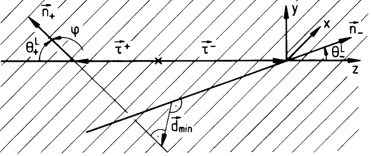
Figure 3: Kinematic configuration indicating the relative orientation of the hadronic tracks, the $\tau$ directions and the vector $\vec{d}_{min}$.

2 Tau kinematics

In all experimental and theoretical analysis of $\tau$ decays it has been implicitly assumed that the $\tau$ direction and its restframe cannot be fully reconstructed and appropriately averaged distributions are considered. However, as shown in [17], impact parameter measurements allow to fully reconstruct the $\tau$ direction.

In events where both leptons decay semileptonically and where all hadron momenta are determined, the original $\tau$ direction can be reconstructed up to a twofold ambiguity [18, 12, 15], which can be resolved with the help of vertex detectors employed in present experiments. Several possibilities may arise:

i.) If the beam spot is large compared to the typical impact parameter, the production vertex is unknown. Let us assume that both $\tau$ decay into one charged hadron each and that both charged tracks can be measured with high precision. The direction $\vec{d}_{min}$ of the minimal distance between the two nonintersecting charged tracks (Fig.1) resolves the ambiguity and introduces two additional constraints that can be used to reduce the measurement errors. The $\tau^{+}$ and $\tau^{-}$ decay points and their original directions of flight are then uniquely determined.

ii.) Precise knowledge of the beam axis (corresponding to a beam spot of negligible size) leads to a further constraint resulting from the requirement that the reconstructed $\tau$ axis and the beam axis intersect. If the production point would be known in addition then the momenta plus one charged track from the decay of only one $\tau$ would allow to reconstruct the event and double semileptonic decays would lead to a large number of additional constraints.

iii.) If one (or both) $\tau$ decay into several hadrons and if all momenta and two tracks (one from each side) are measured, the same reconstruction can be performed.

Let us first consider case i) where all relevant aspects can be explained most clearly. The angles $\theta^{L}_{\pm}$ between the $\tau^{\pm}$ and the hadron $h^{\pm}$ directions respectively as defined in the lab frame are given by the energies of $h^{+}$ and $h^{-}$ [12]:

$$\cos\theta^{L}_{-}=\frac{\gamma x_{-}-(1+r^{2}_{-})/2\gamma}{\beta\sqrt{\gamma^{2}x_{-}^{2}-r_{-}^{2}}}$$ (9)

$$\sin\theta^{L}_{-}=\sqrt{\frac{(1-r_{-}^{2})^{2}/4-(x_{-}-(1+r^{2}_{-})/2)^{2}/\beta^{2}}{\gamma^{2}x_{-}^{2}-r_{-}^{2}}}$$

$$x_{-}=E_{h^{-}}/E_{\tau}\hskip 56.9055ptr_{-}=m_{h^{-}}/m_{\tau}$$ (10)

and similarly for $\cos\theta^{L}_{+}$ and $\sin\theta^{L}_{+}$. The velocity $\beta$, and the boost factor $\gamma$ refer to the $\tau$ in the lab frame.

The original $\tau^{-}$ direction must therefore lie on the cone of opening angle $\theta^{L}_{-}$ around the direction of $h^{-}$ and on the cone of opening angle $\theta^{L}_{+}$ around the reflected direction of $h^{+}$. The extremal situation where $\theta^{L}_{+}$ or $\theta^{L}_{-}$ assume the values 0 or $\pi$, or where the two cones touch in one line, lead to a unique solution for the $\tau$ direction. In general a twofold ambiguity arises as is obvious from this geometric argument. The cosine of the relative azimuthal angle $\varphi$ between the directions of $h^{+}$ and $h^{-}$ denoted by $\vec{n}_{+}$ and $\vec{n}_{-}$ can be calculated from the momenta and energies of $h^{+}$ and $h^{-}$ as follows: In the coordinate frame (see Fig.1) with the $z$ axis pointing along the direction of $\tau^{-}$ and with $\vec{n}_{-}$ in the $xz$ plane and positive $x$ component

$$\frac{\vec{p}_{-}}{|\vec{p}_{-}|}\equiv\vec{n}_{-}=\left(\begin{array}[]{c}\sin\theta^{L}_{-}\\ 0\\ \cos\theta^{L}_{-}\end{array}\right)$$

$$\frac{\vec{p}_{+}}{|\vec{p}_{+}|}\equiv\vec{n}_{+}=\left(\begin{array}[]{c}\sin\theta^{L}_{+}\cos\varphi\\ \sin\theta^{L}_{+}\sin\varphi\\ -\cos\theta^{L}_{+}\end{array}\right)$$ (11)

and $\cos\varphi$ can be determined from

$$\vec{n}_{-}\vec{n}_{+}=-\cos\theta^{L}_{-}\cos\theta^{L}_{+}+\sin\theta^{L}_{-}\sin\theta^{L}_{+}\cos\varphi$$ (12)

The well-known twofold ambiguity in $\varphi$ is evident from this formula.

Additional information can be drawn from the precise determination of tracks close to the production point. Three-prong decays allow to reconstruct the decay vertex and the ambiguity can be trivially resolved.

However, also single-prong events may serve this purpose. Let us first consider decays into one charged hadron on each side. Their tracks and in particular the vector $\vec{d}_{min}$ of closest approach (Fig.1) can be measured with the help of microvertex detectors. The vector pointing from the $\tau_{-}$ to the $\tau_{+}$ decay vertex

$$\vec{d}\equiv\vec{\tau}_{+}-\vec{\tau}_{-}=-l\left(\begin{array}[]{c}0\\ 0\\ 1\end{array}\right)$$ (13)

is oriented by definition into the negative $z$ direction ($l>0)$. The vector $\vec{d}_{min}$ can on the one hand be measured, on the other hand calculated from $\vec{d}$, $\vec{n}_{+}$ and $\vec{n}_{-}$:

$$\vec{d}_{min}=\vec{d}\,+\,[(\vec{d}\vec{n}_{+}\,\vec{n}_{+}\vec{n}_{-}-\vec{d}\vec{n}_{-})\vec{n}_{-}$$ (15)

$$+(\vec{d}\vec{n}_{-}\,\vec{n}_{+}\vec{n}_{-}-\vec{d}\vec{n}_{+})\vec{n}_{+}]/(1-(\vec{n}_{-}\vec{n}_{+})^{2})$$

The sign of the projection of $\vec{d}_{min}$ on $\vec{n}_{+}\times\vec{n}_{-}$ then determines the sign of $\varphi$ and hence resolves the ambiguity.

$$\vec{d}_{min}(\vec{n}_{+}\times\vec{n}_{-})=l\sin\theta^{L}_{+}\sin\theta^{L}_{-}\sin\varphi$$ (16)

The length of the projection determines $l$ and hence provides a measurement of the lifetimes of $\tau_{+}$ plus $\tau_{-}$. Exploiting the fact that $\vec{d}\vec{n}_{-}=-l\cos\theta^{L}_{-}$ and $\vec{d}\vec{n}_{+}=l\cos\theta^{L}_{+}$ the direction of $\vec{d}$ can be geometrically constructed by inverting (15):

$$\vec{d}/l=\vec{d}_{min}/l\,-\,[(\cos\theta^{L}_{+}\,\vec{n}_{+}\vec{n}_{-}+\cos\theta^{L}_{-})\vec{n}_{-}+$$

$$(-\cos\theta^{L}_{-}\,\vec{n}_{+}\vec{n}_{-}-\cos\theta^{L}_{+})\vec{n}_{+}]/(1-(\vec{n}_{-}\vec{n}_{+})^{2})$$

In addition two constraint equations may be derived by comparing $\vec{d}_{min}/l$ as calculated from the $h_{+}$ and $h_{-}$ tracks with the direction calculated from (15) with the help of $\theta^{L}_{+}$, $\theta^{L}_{-}$ and $l$. These might be used to constrain the events even in cases where initial state radiation distorts the simple kinematics described above.

As stated before, the locations of both $\tau_{+}$ and $\tau_{-}$ decay vertices in space are then fixed. If the beam axis is known with high precision (high compared to the decay length $l$) the lines between the two decay vertices and the beam axis intersect, providing one additional constraint.

The generalization of this method to decays into multihadron states with one or several neutrals is straightforward: $\theta^{L}_{+}$, $\theta^{L}_{-}$ and $\cos\varphi$ are fixed by the hadron momenta as stated above. Only one of the two solutions for $\varphi$ is then compatible with $\vec{d}_{min}$ measured directly with the help of vertex detectors.

3 $\tau$-polarization

As discussed in chapter 1, the technique of structure functions serves as a usefull tool to analyse the hadronic current and the $\tau$-polarization. Once the $\tau$ restframe is reconstructed one may also proceed in a more direct way which allows to exploit maximally the spin information on an event by event basis.

The current $J_{\mu}$ depends generically on all hadron momenta. In [12] it has been demonstrated that the direction of the $\tau$-spin in the $\tau$-restframe in each event is given by

$$\vec{h}=\vec{H}/\omega$$ (18)

with

$$\omega=P^{\mu}(\Pi_{\mu}-\Pi^{5}_{\mu});~{}~{}~{}~{}~{}\vec{H}=m_{\tau}(\vec{\Pi}^{5}-\vec{\Pi})$$ (19)

$$\Pi_{\mu} = 2[(J^{*}\cdot N)J_{\mu}+(J\cdot N)J^{*}_{\mu}-(J^{*}\cdot J)N_{\mu}];$$

$$\Pi^{5}_{\mu} = 2\,{\rm Im}\,\epsilon_{\mu}^{\phantom{\mu}\nu\rho\sigma}J_{\nu}^{*}J_{\rho}N_{\sigma}.$$ (20)

The momenta $P$ and $N$ refer to the $\tau$ and its neutrino. The $V-A$ structure of the lepton current and a massless neutrino have been assumed for simplicity.

For the decay into a single pion $J_{\mu}\propto Q_{\mu}$ and the direction of the vector $\vec{h}$ is identical to that of the momentum of the pion, its normalization equal to one. For the decay into several pions the current $J_{\mu}$ and consequently the direction of $h$ will depend on all pion momenta. It is, however, a simple exercise to demonstrate that

$$\vec{h}^{2}=1\,$$ (21)

also in the general case. This follows directly from

$$(\Pi_{\mu}-\Pi_{\mu}^{5})(\Pi^{\mu}-\Pi^{5\mu})=0$$ (22)

and is a direct consequence of the $V-A$ coupling at the lepton vertex and of the fact that no spin summation has been performed for the hadronic system. Also decay modes with kaons or $\eta$’s only have maximal analysing power, corresponding to $|\vec{h}|=1$.

The argument is in particular also applicable for $\tau\to\nu\pi\omega(\to 3\pi)$ if all four pion momenta are measured and the full matrix element including also the $\omega\to 3\pi$ decay is used for the hadronic current. The argument would fail, if the spin of the $\omega$ meson would be averaged. Correspondingly, $|\vec{h}|\neq 1$ for leptonic decay modes.

However, one important assumption has been made tacidly throughout: The form of the current must be known for the analysis of multi-hadron states. For 2 pions this form is essentially fixed, for 3 pions it is highly plausible. For multi-meson states, in particular those including kaons, a carefull test of the functional form of $J$ is madatory.

To summarize: Semileptonic decay modes of the $\tau$-lepton carry important information on hadron physics and $\tau$-properties. Measurements of the structure functions are a convenient tool to constrain models and to determine the hadronic current in a model-independent way. Given sufficiently precise vertex detectors, double-semileptonic events can be fully reconstructed. Once the model for the hadronic current is reliable, the $\tau$ spin can be measured in semileptonic decays on an event by event basis.

References

- [1] J.H. Kühn and E. Mirkes, Z. Phys. C 56 (1992) 661.
- [2] J.H. Kühn and A. Santamaria, Z. Phys. C 48 (1990) 445.
- [3] J.H. Kühn and E. Mirkes, Phys. Lett. B 286 (1992) 381.
-
[4]
M. Schmidtler, Proc. Third Workshop
on Tau Lepton Physics,
Montreux 1994. - [5] R. Decker and E. Mirkes, Phys. Rev. D 47 (1993) 4012.
- [6] R. Decker, E. Mirkes, R. Sauer and Z. Was, Z. Phys. C 58 (1993) 445.
-
[7]
R. Decker, Proc. Third Workshop
on Tau Lepton Physics,
Montreux 1994. - [8] J. Wess and B. Zumino, Phys. Lett. B 37 (1971) 95.
- [9] ALEPH Collaboration, Z. Phys. C 59 (1993) 369.
- [10] P. Privitera, Phys. Lett. B 308 (1993) 163.
-
[11]
N. Wermes, Proc. Third Workshop
on Tau Lepton Physics,
Montreux 1994. - [12] J.H. Kühn and F. Wagner, Nucl. Phys. B 236 (1984) 16.
- [13] K. Hagiwara, A.D. Martin and D. Zeppenfeld, Phys. Lett. B 235 (1990) 198.
-
[14]
A. Rougé, First Workshop on Tau Lepton Physics, Orsay 1990,
M. Davier and B. Jean-Marie, eds, Editions Frontiéres(1991)213.
A. Rougé, Z. Phys. C 48 (1990) 75. - [15] M. Davier, L. Duflot, F. Le Diberder, A. Rougé Phys. Lett. B 306 (1993) 411.
- [16] R. Decker and E. Mirkes, Z. Phys. C 57 (1993) 495.
- [17] J.H. Kühn, Phys. Lett. B 313 (1993) 458.
- [18] P. Tsai and A.C. Hearn, Phys. Rev. 140 (1965) 721.