Bounds on the Higgs mass in the Standard Model and Bounds on the Higgs mass in the Standard Model and Minimal Supersymmetric Standard Model

We present bounds on the Higgs mass in the Standard Model and in the Minimal Supersymmetric Standard Model using the effective potential with next-to-leading logarithms resummed by the renormalization group equations, and physical (pole) masses for the top quark and Higgs boson. In the Standard Model we obtain lower bounds from stability requirements: they depend on the top mass and the cutoff scale. In the Minimal Supersymmetric Standard Model we obtain upper bounds which depend on the top mass and the scale of supersymmetry breaking. A Higgs mass measurement could discriminate, depending on the top mass, between the two models. Higgs discovery at LEP-200 can put an upper bound on the scale of new physics.

CERN–TH.7507/94

November 1994

CERN–TH.7507/94

IEM–FT–95/94

hep-ph/9411403

BOUNDS ON THE HIGGS MASS IN THE STANDARD MODEL AND

MINIMAL SUPERSYMMETRIC STANDARD MODEL

MARIANO QUIROS

TH Division, CERN, CH-1211

Geneva 23, Switzerland

ABSTRACT

We present bounds on the Higgs mass in the Standard Model and in the Minimal Supersymmetric Standard Model using the effective potential with next-to-leading logarithms resummed by the renormalization group equations, and physical (pole) masses for the top quark and Higgs boson. In the Standard Model we obtain lower bounds from stability requirements: they depend on the top mass and the cutoff scale. In the Minimal Supersymmetric Standard Model we obtain upper bounds which depend on the top mass and the scale of supersymmetry breaking. A Higgs mass measurement could discriminate, depending on the top mass, between the two models. Higgs discovery at LEP-200 can put an upper bound on the scale of new physics.

1 Introduction

In view of Higgs searches at future colliders (in particular at LEP-200) it is extremely important to compute theoretical bounds on the Higgs mass as accurately as possible. Indeed, the very measurement of the Higgs mass, apart from confirming our knowledge of renormalizable field theories, can shed some light on the particular model that Nature has chosen at the TeV scale.

The two most appealing models are: the Standard Model (SM), which is being confirmed at LEP with $\sim$ 1% precision, and its minimal supersymmetric extension, the Minimal Supersymmetric Standard Model (MSSM), which is very well motivated theoretically (it helps in technically solving the gauge hierarchy problem) but has received no experimental support from present colliders (TEVATRON, LEP). On the contrary what present colliders are doing is to establish lower bounds on all supersymmetric parameters, and therefore sending the scale of supersymmetry breaking to higher values.

The direct confirmation or exclusion of the MSSM will probably have to wait for the LHC. In the meantime, while present and future accelerators will continue to rise the bounds on supersymmetric parameters, we would like to know whether the discovery of the Higgs boson and the measurement of its mass could, apart from confirming the SM, give information about the possibility that the SM is embedded in an extended electroweak theory: in particular the MSSM. On the one hand, if all supersymmetric parameters are at the TeV scale, the lightest Higgs boson of the MSSM should have the same couplings to ordinary matter than the SM Higgs. On the other hand LEP-200 will cover a range of Higgs masses up to $\sim M_{Z}$ and direct detection of supersymmetry will not happen if supersymmetric masses are not $\stackrel{{\scriptstyle<}}{{{}_{\sim}}}M_{Z}$. If this is the case, the best tool LEP-200 will have to uncover new physics is through the Higgs search and the measurement of its mass.

In this talk we will review the theoretical knowledge we have on the SM Higgs mass and on the MSSM lightest Higgs boson mass. In Section 2 we will present lower bounds on the SM Higgs mass from the requirement of stability of the effective potential, i.e. from the requirement that we do not live in a metastable minimum. We will see that it imposes strong lower bounds on the mass of the Higgs boson, $M_{H}$, which will be a function of the top mass $M_{t}$ and of the SM cutoff $\Lambda$. In Section 3 we will review the upper bounds on the lightest Higgs boson mass $M_{H}$ that will depend on various supersymmetric parameters and $M_{t}$. In Section 4 we will draw some conclusions concerning the possible detection of the Higgs at LEP-200.

2 Lower bounds in the Standard Model: stability bounds

The vacuum stability requirement in the SM imposes a severe lower bound on the mass of the Higgs boson $M_{H}$ ^1-5, which depends on the mass of the top quark $M_{t}$ and on the cut-off $\Lambda$ beyond which the SM is no longer valid. Roughly speaking, this is due to the fact that the top Yukawa coupling $h_{t}$ drives the quartic coupling of the Higgs potential $\lambda$ from its initial value at $M_{Z}$ (which determines the Higgs mass) to negative values at large scales, thus destabilizing the standard electroweak vacuum.

In previous works, the stability bound was obtained from the tree level potential, improved by one-loop or two-loop renormalization group equations (RGE) for the $\beta$- and $\gamma$-functions of the running couplings, masses and the $\phi$-field ^?,?. However, it has been shown that the one-loop corrections to the Higgs potential are important in order to fix the boundary conditions for the electroweak breaking and calculate the Higgs mass in a consistent and scale-independent way. As we will see, they are also significant to properly understand the whole structure of the potential. Typically we find that the lower bound on $M_{H}$ is ${\cal O}$(10 GeV) lower than in previous estimates ^?.

The renormalization group improved effective potential of the SM, $V$, can be written in the ’t Hooft-Landau gauge and the $\overline{MS}$ scheme as ^?

$$V[\mu(t),\lambda_{i}(t);\phi(t)]\equiv V_{0}+V_{1}+\cdots\;\;,$$ (1)

where $\lambda_{i}\equiv(g,g^{\prime},\lambda,h_{t},m^{2})$ runs over all dimensionless and dimensionful couplings, and $V_{0}$, $V_{1}$ are respectively the tree level potential and the one-loop correction, namely

$$V_{0}=-{\displaystyle\frac{1}{2}}m^{2}(t)\phi^{2}(t)+{\displaystyle\frac{1}{8}}\lambda(t)\phi^{4}(t),$$ (2a)

$$V_{1}={\displaystyle\sum_{i=1}^{5}}{\displaystyle\frac{n_{i}}{64\pi^{2}}}M_{i}^{4}(\phi)\left[\log{\displaystyle\frac{M_{i}^{2}(\phi)}{\mu^{2}(t)}}-c_{i}\right]+\Omega(t),$$ (2b)

where $M_{i}^{2}(\phi,t)=\kappa_{i}\phi^{2}(t)-\kappa_{i}^{\prime}$ (1 $\equiv$ $W$, 2 $\equiv$ $Z$, 3 $\equiv$ top, 4 $\equiv$ Higgs and 5 $\equiv$ Goldstones) are the tree-level expressions for the masses of the particles that enter in the one-loop radiative corrections, and $n_{1}=6$, $\kappa_{1}=\frac{1}{4}g^{2}(t)$, $\kappa_{1}^{\prime}=0$, $c_{1}=\frac{5}{6}$; $n_{2}=3$, $\kappa_{2}=\frac{1}{4}[g^{2}(t)+g^{\prime 2}(t)]$, $\kappa_{2}^{\prime}=0$, $c_{2}=\frac{5}{6}$; $n_{3}=-12$, $\kappa_{3}=\frac{1}{2}h_{t}^{2}(t)$, $\kappa_{3}^{\prime}=0$, $c_{3}=\frac{3}{2}$; $n_{4}=1$, $\kappa_{4}=\frac{3}{2}\lambda(t)$, $\kappa_{4}^{\prime}=m^{2}(t)$, $c_{4}=\frac{3}{2}$; $n_{5}=3$, $\kappa_{5}=\frac{1}{2}\lambda(t)$, $\kappa_{5}^{\prime}=m^{2}(t)$, and $c_{5}=\frac{3}{2}$. $\Omega(t)\equiv\Omega[\lambda_{i}(t),\mu(t)]$ is the one-loop contribution to the cosmological constant ^?, which will turn out to be irrelevant in our calculation.

In the previous expressions the parameters $\lambda(t)$ and $m(t)$ are the SM quartic coupling and mass, whereas $g(t)$, $g^{\prime}(t)$, $h_{t}(t)$ are the SU(2), U(1) and top Yukawa couplings respectively. All of them are running with the RGE. The running of the Higgs field is $\phi(t)=\xi(t)\phi_{c}$, $\phi_{c}$ being the classical field and $\xi(t)=\exp\{-\int^{t}_{0}\gamma(t^{\prime})dt^{\prime}\}$, where $\gamma(t)$ is the Higgs field anomalous dimension. Finally the scale $\mu(t)$ is related to the running parameter $t$ by $\mu(t)=\mu e^{t}$, where $\mu$ is a fixed scale, we will take equal to the physical $Z$ mass, $M_{Z}$.

It has been shown ^? that the $L$-loop effective potential improved by ($L$+1)-loop RGE resums all $L$th-to-leading logarithm contributions. Consequently, we will consider all the $\beta$- and $\gamma$-functions of the previous parameters to two-loop order, so that our calculation will be valid up to next-to-leading logarithm approximation.

As has been pointed out ^?, working with $\partial V/\partial\phi$ (and higher derivatives) rather than with $V$ itself allows us to ignore the cosmological constant  aterm $\Omega$. In fact, the structure of the potential can be well established once we have determined the values of $\phi$, say $\phi_{{\mathrm{e}xt}}$, in which $V$ has extremals (maxima or minima). Thus we only need to evaluate $\partial V/\partial\phi$ and $\partial^{2}V/\partial\phi^{2}$.

The structure of maxima and minima of $V$ for large $\phi$ can be evaluated at a scale $\mu(t)$ within the region where $V$ is scale-invariant. As was previously discussed ^?, $\mu(t)=\phi(t)$ is always a correct choice (other choices, such that $\mu(t)=\phi(t)/2$, are equally valid and lead to essentially the same results). Then the extremal condition, neglecting the Higgs and Goldstone contributions, reads ^?

$$\phi^{2}_{{\mathrm{e}xt}}=\frac{2m^{2}}{\tilde{\lambda}},$$ (3)

$$\tilde{\lambda} = \lambda-{\displaystyle\frac{1}{16\pi^{2}}}\left\{6h_{t}^{4}\left[\log{\displaystyle\frac{h_{t}^{2}}{2}}-1\right]-{\displaystyle\frac{3}{4}}g^{4}\left[\log{\displaystyle\frac{g^{2}}{4}}-{\displaystyle\frac{1}{3}}\right]\right.$$ (4)

$$- \left.{\displaystyle\frac{3}{8}}\left(g^{2}+g^{\prime 2}\right)^{2}\left[\log{\displaystyle\frac{\left(g^{2}+g^{\prime 2}\right)}{4}}-{\displaystyle\frac{1}{3}}\right]\right\},$$

[all quantities in (3,4) are evaluated at $\mu(t)=\phi_{{\mathrm{e}xt}}(t)$]. From (3) we see that, if $V$ develops an extremal for large values of $\phi$, this must occur for a value of $\phi$ such that

$$0<\tilde{\lambda}[\mu(t)=\phi(t)]\ll 1.$$ (5)

On the other hand, for large values of $\phi$ the second derivative of the potential (1) can be very accurately expressed as ^?

$$\left.\frac{\partial^{2}V}{\partial\phi^{2}(t)}\right|_{\phi(t)=\phi_{{\mathrm{e}xt}}(t)} = \frac{1}{2}(\beta_{\lambda}-4\gamma\lambda)\phi^{2}(t),$$ (6)

where $\beta_{\lambda}$ is the one-loop $\beta$-function. Since near the extremum $\lambda$ is very small, we see from (6) that depending on the sign of $\beta_{\lambda}$ we will have a maximum or a minimum.

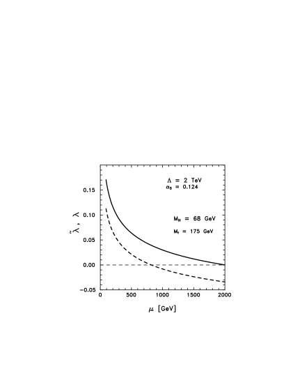
Figure 1: Plot of $\lambda$ (dashed line) and $\tilde{\lambda}$ (solid line) as a function of the scale $\mu(t)$ for $M_{t}=175$ GeV, $\Lambda=2$ TeV, $M_{H}=68$ GeV and $\alpha_{S}=0.124$.

We have illustrated these features in Fig. 1 with a typical example. It represents the evolution of $\lambda$ (dashed line) and $\tilde{\lambda}$ (solid line) with $\mu(t)$. It is worth noticing that they do not cross the horizontal axis at the same value of $\mu(t)$, but they differ by a relatively large amount. This is important since the point where the maximum of the potential is located, say $\phi_{MAX}$, does correspond ^? to $\tilde{\lambda}\sim 0$ rather than ${\lambda}\sim 0$. This is so in Fig. 2, where the scalar potential, $V(\phi)$, has been represented for a typical choice of parameters. Notice that for values of $\phi$ very slightly higher than $\phi_{MAX}$, the potential is negative and much deeper than the electroweak minimum. This is simply because for values of $\mu(t)$ just beyond $\mu_{MAX}=\phi_{MAX}$, the value of $\tilde{\lambda}$ becomes negative and the potential is dominated by the contribution $\frac{1}{8}\tilde{\lambda}\phi^{4}$. Consequently, a sensible criterion for a model to be safe is to require one of the two following conditions: a) The potential has no maximum; b) The maximum occurs for $\phi_{M}>\Lambda$. In the following we will assume $\Lambda\leq 10^{19}$ GeV. With this criterion [in particular condition (b)] we see that the model represented in Fig. 2 is acceptable for $\Lambda\leq 2.7\times 10^{11}$ GeV. Beyond this scale, the stability of the vacuum requires the appearance of new physics. Note from this discussion that conditions (a), (b) are not equivalent to require $\lambda(\mu)>0$ for $\mu(t)<\Lambda$, as is usually done. Instead, the significant parameter is $\tilde{\lambda}$ rather than ${\lambda}$.

Figure 2: Plot of the effective potential $V(\phi)$ corresponding to $M_{t}=160$ GeV, $M_{H}=100$ GeV, $\alpha_{S}=0.124$ and $\Lambda=10^{19}$ GeV, represented in a convenient choice of units.

The running Higgs mass, $m_{H}^{2}(t)$, defined as the curvature of the scalar potential at the minimum, can be readily obtained from

$$m_{H}^{2}(t^{*})=\left.\frac{\partial^{2}V}{\partial\phi^{2}(t^{*})}\right|_{\phi(t^{*})=\langle\phi(t^{*})\rangle},$$ (7)

where $t^{*}$ is the scale at which we define the electroweak minimum ^?. The scale invariance of the second derivative of the potential, $\frac{\partial}{\partial t}\left[\xi^{2}(t)\frac{\partial^{2}V}{\partial\phi^{2}(t)}\right]=0$, allows us to write $m_{H}^{2}(t)$ at any arbitrary scale

$$m_{H}^{2}(t)=m_{H}^{2}(t^{*}){\displaystyle\frac{\xi^{2}(t^{*})}{\xi^{2}(t)}}.$$ (8)

The physical (pole) Higgs mass, $M_{H}^{2}$, is then given by

$$M_{H}^{2}=m_{H}^{2}(t)+{{\mathrm{R}e}}[\Pi(p^{2}=M_{H}^{2})-\Pi(p^{2}=0)],$$ (9)

where $\Pi(p^{2})$ is the renormalized self-energy of the Higgs boson ^? (the $t$-dependence drops out from (9)).

Figure 3: SM lower bound on $M_{H}$ as a function of $M_{t}$ for $\alpha_{S}(M_{Z})=0.124$ and different values of $\Lambda$ in the range $10^{3}$ GeV $\leq\Lambda\leq 10^{19}$ GeV. The values of $\Lambda$ for consecutive curves differ by two orders of magnitude.

As has been stated above, the choice of $\mu^{*}$, i.e. the scale at which we evaluate the minimum conditions, is not important for physical quantities, provided it is within a (quite wide) region around the optimal value ^?. The lack of flatness of $M_{H}$ reflects the effect of all non-considered (higher-order) contributions in the calculation and, therefore, it is a measure of the total error in our estimate of $M_{H}$. We deduced ^? that the error is typically $\stackrel{{\scriptstyle<}}{{{}_{\sim}}}$ 3 GeV, which is the uncertainty we should assign to our results. Had we performed the previous calculations just with the (RGE-improved) tree-level part of $V$ in Eq. (1) ^?,?, the Higgs mass would have a strong dependence on $\mu^{*}$. Choosing ^?,? $\mu^{*}=M_{Z}$ results in an error in the estimate of $M_{H}$, whose precise value depends on the top mass and is typically of ${\cal O}(10\ {{\mathrm{G}eV}})$, showing the need of a more careful treatment of the problem, as the one exposed above ^?.

Finally, let us note that in the previous equations the top Yukawa coupling $h_{t}(t)$ enters in several places. Therefore, the Higgs mass depends on the boundary condition chosen for $h_{t}(t)$, and thus on the top mass $M_{t}$. However the running top mass, defined as $m_{t}(t)=vh_{t}(t)$, does not coincide with the physical (pole) mass $M_{t}$. In the Landau gauge the relationship between the running $m_{t}$ and the physical (pole) mass $M_{t}$ is given by ^?

$$M_{t}=\left\{1+{\displaystyle\frac{4}{3}}{\displaystyle\frac{\alpha_{S}(M_{t})}{\pi}}+\left[16.11-1.04\sum_{i=1}^{5}\left(1-\frac{M_{i}}{M_{t}}\right)\right]\left(\frac{\alpha_{S}(M_{t})}{\pi}\right)^{2}\right\}m_{t}(M_{t}),$$ (10)

where $M_{i}$, $i=1,\ldots,5$ represent the masses of the five lighter quarks.

As has become clear from the previous discussion, the lower bound on $M_{H}$ is a function of $M_{t}$ and $\Lambda$. However, apart from the previously estimated error $\stackrel{{\scriptstyle<}}{{{}_{\sim}}}$ 3 GeV in our calculation, there is an additional source of uncertainty coming from the value of $\alpha_{s}$, which enters in several places in the previous calculation. The most recent estimate of $\alpha_{s}$ gives

$$\alpha_{s}=0.124\pm 0.006.$$ (11)

Using the central value of (11), we have represented in Fig. 3 the lower bound on $M_{H}$ as a function of $M_{t}$ for different values of $\Lambda$. The form of the curves is easily understandable from the previous discussion. In Fig. 4, we have fixed $\Lambda$ at its maximum value, $\Lambda=10^{19}$ GeV, and represented the lower bound on $M_{H}$ for the central value of $\alpha_{s}$ in (11) (diagonal solid line) and the two extreme values (diagonal dashed lines).

If we use the recent evidence for the top quark production at CDF with a mass $M_{t}=174\pm 17$ GeV ^?, we obtain the following lower bound on $M_{H}$:

$$M_{H}>128\pm 33\ {{\mathrm{G}eV}},$$ (12)

i.e. $M_{H}>$ 95 GeV (1$\sigma$). If the Higgs is observed in the present or forthcoming accelerators with a mass below the bound of Eq. (12), this would be a clear signal of new physics beyond the SM.

Comparing these bounds with previous evaluations ^?, we see that our values of $M_{H}$ are lower by an amount increasing with $M_{t}$, going from $\sim 5$ GeV for $M_{t}\sim$ $130$ GeV to $\sim 15$ GeV for $M_{t}\sim 200$ GeV. As has been discussed previously the main reason of this difference is the way in which the Higgs mass was previously computed ^?. Accordingly, our results give more room to the Higgs mass in the framework of the Standard Model.

3 Upper bounds in the Minimal Supersymmetric Standard Model

The MSSM has an extended Higgs sector with two Higgs doublets with opposite hypercharges: $H_{1}$, responsible for the mass of the charged leptons and the down-type quarks, and $H_{2}$, which gives a mass to the up-type quarks. After the Higgs mechanism there remain three physical scalars, two CP-even and one CP-odd Higgs bosons. In particular, the lightest CP-even Higgs boson mass satisfies the tree-level bound

$$m_{H}^{2}\leq M_{Z}^{2}\cos^{2}2\beta,$$ (13)

where $\tan\beta=v_{2}/v_{1}$ is the ratio of the Vacuum Expectation Values (VEVs) of the neutral components of the two Higgs fields $H_{2}$ and $H_{1}$. Relation (13) implies that $m_{H}^{2}<M_{Z}^{2}$, for any value of $\tan\beta$, which, in turn, implies that it should be found at LEP-200 ^?. However, the tree-level relation (13) is spoiled by one-loop radiative corrections, which were computed by several groups using: the effective potential approach ^?, diagrammatic methods ^? and renormalization group (RG) techniques ^?. All methods found excellent agreement with one another and large radiative corrections, mainly controlled by the top Yukawa coupling, which could make the lightest CP-even Higgs boson escape experimental detection at LEP-200. In particular, the RG approach (which will be followed in this talk) is based on the fact that supersymmetry decouples and, below the scale of supersymmetry breaking $M_{S}$, the effective theory is the SM, with some matching conditions at $M_{S}$. Assuming $M_{Z}^{2}\ll M_{S}^{2}$ the tree-level bound (13) is saturated at the scale $M_{S}$ and the effective SM at scales between $M_{Z}$ and $M_{S}$ contains the Higgs doublet $H=H_{1}\cos\beta+i\sigma_{2}H_{2}^{*}\sin\beta$, with a quartic coupling taking, at the scale $M_{S}$, the (tree-level) value of

$$\lambda={\displaystyle\frac{1}{4}}(g^{2}+g^{\prime 2})\cos^{2}2\beta.$$ (14)

In these analyses ^? the Higgs mass was considered at the tree level, improved by one-loop renormalization group equations (RGE) in the $\gamma$- and $\beta$-functions, thus collecting all leading logarithm corrections.

Since the relative size of one-loop corrections to the Higgs mass is large (mainly for large top quark mass and/or small tree-level Higgs mass) it was compelling to analyse them at the two-loop level. A first step in that direction was given some time ago ^? where two-loop RGE-improved tree-level Higgs masses were considered. It was found that two-loop corrections were negative and small. The Higgs mass received all leading logarithm and part of the next-to-leading logarithm corrections ^?. As we have described in Section 2, for fully taking into account all next-to-leading logarithm corrections the one-loop effective potential (improved by two-loop RGE) is needed.

The tree-level quartic coupling (14) receives one-loop threshold contributions at the $M_{S}$ scale. These are given by

$$\Delta\lambda={\displaystyle\frac{3h_{t}^{4}}{16\pi^{2}}}{\displaystyle\frac{X_{t}^{2}}{M_{S}^{2}}}\left(2-{\displaystyle\frac{X_{t}^{2}}{6M_{S}^{2}}}\right),$$ (15)

where $h_{t}$ is the top Yukawa coupling in the SM and $X_{t}=A_{t}+\mu\cot\beta$ is the stop mixing.

The correction (15) has a maximum for $X_{t}^{2}=6M_{S}^{2}$. For that reason, in our numerical applications we will take $X_{t}^{2}=6M_{S}^{2}$, i.e. maximal threshold effect. Notice also that $X_{t}^{2}=6M_{S}^{2}$ is barely consistent with the bound from colour-conserving minimum ^?, so that the case of maximal threshold really represents a particularly extreme situation. In addition to the previous effect, there appear effective higher-order operators ($D\geq 6$), which for $M_{S}\geq 1$ TeV turn out to be negligible ^?.

Upper bounds on the lightest Higss boson mass in the MSSM depend therefore on three supersymmetric parameters (besides $M_{t}$): $M_{S}$ (from naturality reasons $M_{S}\stackrel{{\scriptstyle<}}{{{}_{\sim}}}1$ TeV ^?), $\tan\beta$ and $X_{t}=A_{t}+\mu/\tan\beta$, which is responsible for the threshold correction to the Higgs quartic coupling. The larger the threshold correction and $\tan\beta$, the less stringent the supersymmetric bounds. Therefore, the most conservative situation takes place considering maximum threshold correction (which is achieved for $X_{t}^{2}=6M_{S}^{2}$) and $\tan\beta=\infty$. Likewise, the larger $M_{S}$, the less stringent the bounds; but, as mentioned above, it is not sensible to consider $M_{S}$ much larger than $1$ TeV. Consequently, to be on the safe side, we have represented in Fig. 4 the MSSM upper bounds (transverse solid and dashed lines), as recently obtained up to next-to-leading-log order ^?, in the most conservative situation with $M_{S}=1$ TeV.

Figure 4: Diagonal (thick) lines: SM lower bound on $M_{H}$ as a function of $M_{t}$ for $\Lambda=10^{19}$ GeV and $\alpha_{s}=0.124$ (solid line), $\alpha_{s}=0.118$ (upper dashed line), $\alpha_{s}=0.130$ (lower dashed line). Transverse (thin) lines: MSSM upper bounds on $M_{H}$ for $\Lambda_{S}=1$ TeV and $\alpha_{s}$ as in the diagonal lines.

Two papers have recently tried to incorporate radiative corrections to the Higgs mass up to the next-to-leading order, and with qualitatively different results. Using the RG approach, positive and large next-to-leading corrections, with respect to the one-loop results, were found by Kodaira, Yasui and Sasaki (KYS) ^?. Using diagrammatic and effective potential methods in a particular MSSM, as well as various approximations, Hempfling and Hoang (HH) ^? found that two-loop corrections are also sizeable, but negative with respect to the one-loop result! Using the RG approach, we have found ^? that two-loop corrections are negative with respect to the one-loop result. We have traced back the origin of this disagreement with KYS ^? in their choice of the minimization scale. Furthermore KYS neglected various effects (as the contribution of gauge bosons to the one-loop effective potential, or the wave function renormalization of top quark and Higgs boson) and considered only the case with zero stop mixing. On the other hand, we have found that the abnormal size of the two-loop corrections obtained by HH ^? is a consequence of an excessively rough estimate of the one-loop result, but we are in agreement with their final two-loop result. In fact our two-loop results differ from those of HH ^? by less than $3\%$. Also our results show a large sensitivity of the Higgs mass to the stop mixing parameter.

Finally we would like to comment briefly on the generality of our results. As was already stated, we are assuming average squark masses $M_{S}^{2}\gg M_{Z}^{2}$, and that all supersymmetric particle masses are $\stackrel{{\scriptstyle>}}{{{}_{\sim}}}M_{S}$. If we relax the last assumption, i.e. if some supersymmetric particles were much lighter, the value of the quartic coupling at $M_{S}$ (see Eq. (14)) would be slightly increased and, correspondingly, our bounds would be slightly relaxed. We have made an estimate of this effect. Assuming an extreme case where all gauginos, higgsinos and sleptons have masses $\sim M_{Z}$, we have found for $M_{S}=1$ TeV and $\cos^{2}2\beta=1$ an increase of the Higgs mass $\sim 2\%$. For values of $\tan\beta$ close to 1 (as those appearing in infrared fixed point scenarios) the corresponding effect is negligible. On the other hand, our numerical results have been computed for $M_{S}=1$ TeV. For values of $M_{S}<1$ TeV the bounds on the lightest Higgs mass are lowered. Hence, in this sense, all our results can be considered as absolute upper bounds.

4 Conclusions

We want to conclude with comments on the two questions we raised at the beginning of this talk: i) Can the Higgs mass measurement disentangle between the SM and the MSSM? ii) Can eventually a Higgs mass measurement at LEP-200 help in putting upper bounds on the scale of new physics?

As for question i), a quick glance at Fig. 4 shows that for $M_{t}=173\pm 4$ GeV, i.e. the crossing area of the SM and MSSM curves, the Higgs mass eventually measured will be compatible either with the pure SM or with the MSSM, but not with both at the same time. Accordingly, the experimental Higgs mass either will discard the MSSM or will be a clear signal of new physics beyond the SM compatible with the MSSM. For $M_{t}<169$ GeV, the situation is analogous, but there is a wider range of Higgs masses (area within the two curves) compatible with both SM and MSSM. For $M_{t}>177$ GeV, there is no region of Higgs masses simultaneously compatible with the SM and MSSM. On the contrary there is a range of $M_{H}$ (within the two curves) that would discard both. This means that for $M_{t}>M_{t}^{c}=177$ GeV a Higgs mass measurement could always discriminate between the SM and the MSSM. This statement has two caveats: one is that it is based upon assuming that the SM holds up to the Planck scale. Had we considered the validity of the SM up to a lower scale, we should have obtained a value $M_{t}^{c}>177$ GeV, with a larger overlapping region where the Higgs mass measurement cannot discriminate between the SM and MSSM. The second caveat is that we are requiring absolute stability for the effective potential: instead, the requirement of metastability of the electroweak minimum will decrease the lower bound and go along the same direction as the previous effect. A detailed calculation along these lines is at present being performed.

Figure 5: SM lower bound on $M_{H}$ as a function of $M_{t}$ for $\alpha_{s}(M_{Z})=0.124$ and different values of $\Lambda$ in the range $10^{3}$ GeV $\leq\Lambda\leq 10^{19}$ GeV. Thick lines correspond to $\Lambda=10^{3},\ 10^{4},\ 10^{5}$ and $10^{19}$ GeV. Thin lines correspond to $\Lambda\equiv$1.5, 2, 3, 4, 6 and 8 TeV.

As for question ii), we can see from Fig. 5 that an upper bound on the scale of new physics can be deduced from the Higgs mass measurement. For instance, if $M_{H}<M_{Z}$, and fixing $M_{t}\sim 175$ GeV, we obtain from Fig. 5 that $\Lambda\stackrel{{\scriptstyle<}}{{{}_{\sim}}}10$ TeV. This bound crucially depends on the value of the top mass and will be softened by the second (metastability bound) effect just mentioned.

5 Acknowledgements

I want to express my deepest gratitude to my collaborators on the topics covered by this talk, Alberto Casas, José Ramón Espinosa and Antonio Riotto. I also acknowledge discussions with Marcela Carena, Gordy Kane, Santi Peris, Nir Polonsky, Stephan Pokorski, Carlos Wagner and Fabio Zwirner. I finally wish to thank Fabio Zwirner for a careful reading of the manuscript.

6 References

References

- [1] N. Cabibbo, L. Maiani, G. Parisi and R. Petronzio, Nucl. Phys. B158 (1979) 295.
- [2] M. Lindner, Z. Phys. C31 (1986) 295; M. Sher, Phys. Rep. 179 (1989) 273; M. Lindner, M. Sher and H.W. Zaglauer, Phys. Lett. B228 (1989) 139.
- [3] M. Sher, Phys. Lett. B317 (1993) 159; Addendum: [hep-ph/9404347].
- [4] C. Ford, D.R.T. Jones, P.W. Stephenson and M.B. Einhorn, Nucl. Phys. B395 (1993) 17.
- [5] G. Altarelli and G. Isidori, Phys. Lett. B337 (1994) 141.
- [6] B. Kastening, Phys. Lett. B283 (1992) 287; M. Bando, T. Kugo, N. Maekawa and H. Nakano, Phys. Lett. B301 (1993) 83; Prog. Theor. Phys. 90 (1993) 405.
- [7] J.A. Casas, J.R. Espinosa, M. Quirós and A. Riotto, preprint CERN-TH.7334/94 [hep-ph/9407389], to appear in Nucl. Phys. B.
- [8] J.A. Casas, J.R. Espinosa and M. Quirós, preprint IEM-FT-93/94 [hep-ph/9409458], to appear in Phys. Lett. B.
- [9] N. Gray, D.J. Broadhurst, W. Grafe and K. Schilcher, Z. Phys. C48 (1990) 673.
- [10] F. Abe et al., CDF Collaboration, Phys. Rev. D50 (1994) 2966 and Phys. Rev. Lett. 73 (1994) 225.
- [11] Z. Kunszt and W.J. Stirling, Phys. Lett. B262 (1991) 54.
- [12] Y. Okada, M. Yamaguchi and T. Yanagida, Prog. Theor. Phys. 85 (1991) 1; J. Ellis, G. Ridolfi and F. Zwirner, Phys. Lett. B257 (1991) 83 and B262 (1991) 477; R. Barbieri and M. Frigeni, Phys. Lett. B258 (1991) 395; D. Pierce, A. Papadopoulos and S. Johnson, Phys. Rev. Lett. 68 (1992) 3678.
- [13] H.E. Haber and R. Hempfling, Phys. Rev. Lett. 66 (1991) 1815; A. Yamada, Phys. Lett. B263 (1991) 233; A. Brignole, Phys. Lett. B281 (1992) 284; P.H. Chankowski, S. Pokorski and J. Rosiek, Phys. Lett. B274 (1992) 191.
- [14] Y. Okada, M. Yamaguchi and T. Yanagida, Phys. Lett. B262 (1991) 54; R. Barbieri, M. Frigeni and F. Caravaglios, Phys. Lett. B258 (1991) 167; H.E. Haber and R. Hempfling, Phys. Rev. D48 (1993) 4280.
- [15] J.R. Espinosa and M. Quirós, Phys. Lett. B266 (1991) 389.
- [16] J.M. Frère, D.R.T. Jones and S. Raby, Nucl. Phys. B222 (1983) 11; C. Kounnas, A.B. Lahanas, D.V. Nanopoulos and M. Quirós, Nucl. Phys. B236 (1984) 438; J.-P. Derendinger and C.A. Savoy, Nucl. Phys. B237 (1984) 307; J.A. Casas, A. Lleyda and C. Muñoz, in preparation.
- [17] R. Barbieri and G.F. Giudice, Nucl. Phys. B306 (1988) 63; B. de Carlos and J.A. Casas, Phys. Lett. B309 (1993) 320.
- [18] J. Kodaira, Y. Yasui and K. Sasaki, Hiroshima preprint HUPD-9316, YNU-HEPTh-93-102 (November 1993).
- [19] R. Hempfling and A.H. Hoang, Phys. Lett. B331 (1994) 99.