Bounds on Scalar Leptoquarks from Z Physics

Abstract

We analyse the constraints on scalar leptoquarks coming from radiative corrections to $Z$ physics. We perform a global fitting to the LEP data including the contributions of the most general effective Lagrangian for scalar leptoquarks, which exhibits the $SU(2)_{L}\times U(1)_{Y}$ gauge invariance. We show that the bounds on leptoquarks that couple to the top quark are much stronger than the ones obtained from low energy experiments.

Submitted to Nuclear Physics B

I Introduction

The Standard Model (SM) of electroweak interactions is extremely successful in explaining all the available experimental data [1], which is a striking confirmation of the $SU(2)_{L}\times U(1)_{Y}$ invariant interactions involving fermions and gauge bosons. However, not only has the SM some unpleasant features, like the large number of free parameters, but it also leaves some questions answered, such as the reason for the proliferation of fermion generations and their complex pattern of masses and mixing angles. These problems must be addressed by models that are intended to be more fundamental than the SM. A large number of such extensions of the SM predict the existence of colour triplet particles carrying simultaneously leptonic and baryonic number, the so-called leptoquarks. Leptoquarks are present in models that treat quarks and leptons on the same footing, and consequently quark-lepton transitions are allowed. This class of models includes composite models [2], grand unified theories [3], technicolour models [4], and superstring-inspired models [5].

Since leptoquarks are an undeniable signal for physics beyond the SM, there have been several direct searches for them in accelerators. At the CERN Large Electron-Positron Collider (LEP), the experiments established a lower bound $M_{LQ}\gtrsim 45$–$73$ GeV for scalar leptoquarks [6]. On the other hand, the search for scalar leptoquarks decaying into an electron-jet pair in $p\bar{p}$ colliders constrained their masses to be $M_{LQ}\gtrsim 113$ GeV [7]. Furthermore, the experiments at the DESY $ep$ collider HERA [8] place limits on their masses and couplings, leading to $M_{LQ}\gtrsim 92-184$ GeV depending on the leptoquark type and couplings. There have also been many studies of the possibility of observing leptoquarks in the future $pp$ [9], $ep$ [10, 11], $e^{+}e^{-}$ [12], $e\gamma$ [13], and $\gamma\gamma$ [14] colliders.

One can also constrain the masses and couplings of leptoquarks using the low-energy experiments [15, 16]. For energies much smaller than the leptoquarks mass, they induce two-lepton–two-quark effective interactions that can give rise to atomic parity violation, contributions to meson decay, flavour-changing neutral currents (FCNC), and to meson–anti-meson mixing. However, only leptoquarks that couple to first and second generation quarks and leptons are strongly constrained.

In the present work we study the constraints on scalar leptoquarks that can be obtained from their contributions to the radiative corrections to the $Z$ physics. We evaluated the one-loop contribution due to leptoquarks to all LEP observables and made a global fit in order to extract the 95% confidence level limits on the leptoquarks masses and couplings. The more stringent limits are for leptoquarks that couple to the top quarks. Therefore, our results turn out to be complementary to the low energy limits bounds [15, 16] since these constrain more strongly first and second generation leptoquarks.

The outline of this paper is as follows. In Sec. II we introduce the effective $SU(2)_{L}\times U(1)_{Y}$ invariant effective Lagrangians that we analysed and we also discuss the existing low energy constraints. Section III contains the relevant analytical expressions for the one-loop corrections induced by leptoquarks. Our results and respective discussion are shown in Sec. IV, and we summarize our conclusions in Sec. V. This paper is supplemented with an appendix that contains the relevant Feynman rules.

II Effective Interaction and Their Low Energy Constraints

A natural hypothesis for theories beyond the SM is that they exhibit the gauge symmetry $SU(2)_{L}\times U(1)_{Y}$ above the symmetry breaking scale $v$. Therefore, we imposed this symmetry on the leptoquark interactions. In order to avoid strong bounds coming from the proton lifetime experiments, we required baryon ($B$) and lepton ($L$) number conservation, which forbids the leptoquarks to couple to diquarks. The most general effective Lagrangian for leptoquarks satisfying the above requirements and electric charge and colour conservation is given by [10]

$${\cal L}_{\text{eff}}~{} =~{}{\cal L}_{F=2}~{}+~{}{\cal L}_{F=0}\;,$$ (1)

$${\cal L}_{F=2}~{} =~{}\left(g_{\text{1L}}~{}\bar{q}^{c}_{L}~{}i\tau_{2}~{}\ell_{L}+g_{\text{1R}}~{}\bar{u}^{c}_{R}~{}e_{R}\right)~{}S_{1}+\tilde{g}_{\text{1R}}~{}\bar{d}^{c}_{R}~{}e_{R}~{}\tilde{S}_{1}+g_{3L}~{}\bar{q}^{c}_{L}~{}i\tau_{2}~{}\vec{\tau}~{}\ell_{L}\cdot\vec{S}_{3}\;,$$ (2)

$${\cal L}_{F=0}~{} =~{}h_{\text{2L}}~{}R_{2}^{T}~{}\bar{u}_{R}~{}i\tau_{2}~{}\ell_{L}+h_{\text{2R}}~{}\bar{q}_{L}~{}e_{R}~{}R_{2}+\tilde{h}_{\text{2L}}~{}\tilde{R}^{T}_{2}~{}\bar{d}_{R}~{}i\tau_{2}~{}\ell_{L}\;,$$ (3)

where $F=3B+L$, $q$ ($\ell$) stands for the left-handed quark (lepton) doublet, and $u_{R}$, $d_{R}$, and $e_{R}$ are the singlet components of the fermions. We denote the charge conjugated fermion fields by $\psi^{c}=C\bar{\psi}^{T}$ and we omitted in (2) the flavour indices of the couplings to fermions and leptoquarks. The leptoquarks $S_{1}$ and $\tilde{S}_{1}$ are singlets under $SU(2)_{L}$ while $R_{2}$ and $\tilde{R}_{2}$ are doublets, and $S_{3}$ is a triplet. Furthermore, we assumed in this work that the leptoquarks belonging to a given $SU(2)_{L}$ multiplet are degenerate in mass, with their mass denoted by $M$.

Local invariance under $SU(2)_{L}\times U(1)_{Y}$ implies that leptoquarks also couple to the electroweak gauge bosons. To obtain the couplings to $W^{\pm}$, $Z$, and $\gamma$, we substituted $\partial_{\mu}$ by the electroweak covariant derivative in the leptoquark kinetic Lagrangian:

$${\cal L}_{\text{kin}}=\left(D_{\mu}\Phi\right)^{\dagger}D^{\mu}\Phi\;,$$ (4)

with

$$D_{\mu}\Phi=\left[\partial_{\mu}-i\frac{e}{\sqrt{2}s_{W}}\left(W_{\mu}^{+}T^{+}+W_{\mu}^{-}T^{-}\right)-ieQ_{Z}Z_{\mu}+ieQ^{\gamma}A_{\mu}\right]\Phi\;,$$ (5)

where $\Phi$ stands for the leptoquarks interpolating fields, $Q^{\gamma}$ is the electric charge matrix of the leptoquarks, $s_{W}$ is the sine of the weak mixing angle, and the $T$’s are the generators of $SU(2)_{L}$ for the representation of the leptoquarks. The weak neutral charge $Q_{Z}$ is given by

$$Q_{Z}=\frac{{T_{3}-s_{W}^{2}Q^{\gamma}}}{{s_{W}c_{W}}}\;.$$ (6)

In the last reference of [12], for instance, there is a table with all the quantum numbers for all scalar leptoquarks. In the Appendix we present the Feynman rules for the interactions defined by Eqs. (2) and (4).

Low-energy experiments can lead to strong bounds on the couplings and masses of leptoquarks, due to induced four fermion interactions:

$\bullet$ Leptoquarks can give rise to FCNC processes if they couple to more than one family of quarks or leptons [17, 18]. In order to avoid strong bounds from FCNCs, we assumed that the leptoquarks couple to a single generation of quarks and a single one of leptons. However, due to mixing effects on the quark sector, there is still some amount of FCNC [15] and, therefore, leptoquarks that couple to the first two generations of quarks must comply with some low-energy bounds [15].

$\bullet$ The analyses of the decays of pseudoscalar mesons, like the pions, put stringent bounds on leptoquarks unless their coupling is chiral – that is, it is either left-handed or right-handed [17].

$\bullet$ Leptoquarks that couple to the first family of quarks and leptons are strongly constrained by atomic parity violation [19]. In this case, there is no choice of couplings that avoids the strong limits.

It is interesting to keep in mind that the low-energy data constrain the masses of the first generation leptoquarks to be bigger than $0.5$–$1$ TeV when the coupling constants are equal to the electromagnetic coupling $e$ [15].

III Analytical Expressions

In this work we employed the on-shell-renormalization scheme, adopting the conventions of Ref. [20]. We used as inputs the fermion masses, $G_{F}$, $\alpha_{\text{em}}$, and the $Z$ mass, and the electroweak mixing angle being a derived quantity that is defined through $\sin^{2}\theta_{w}=s_{W}^{2}\equiv 1-M^{2}_{W}/M^{2}_{Z}$. We evaluated the loops integrals using dimensional regularization [21], since it is a gauge-invariant regularization procedure, and we adopted the Feynman gauge to perform the calculations.

Close to the $Z$ resonance, the physics can be summarized by the effective neutral current

$$J_{\mu}=\left(\sqrt{2}G_{\mu}M_{Z}^{2}\rho_{f}\right)^{1/2}\left[\left(I_{3}^{f}-2Q^{f}s_{W}^{2}\kappa_{f}\right)\gamma_{\mu}-I_{3}^{f}\gamma_{\mu}\gamma_{5}\right]\;,$$ (7)

where $Q^{f}$ ($I_{3}^{f}$) is the fermion electric charge (third component of weak isospin). The form factors $\rho_{f}$ and $\kappa_{f}$ have universal contributions, i.e. independent of the fermion species, as well as non-universal parts:

$$\rho_{f} = 1+\Delta\rho_{\text{univ}}+\Delta\rho_{\text{non}}\;,$$ (8)

$$\kappa_{f} = 1+\Delta\kappa_{\text{univ}}+\Delta\kappa_{\text{non}}\;.$$ (9)

Leptoquarks can affect the physics at the $Z$ pole through their contributions to both universal and non-universal corrections. The universal contributions can be expressed in terms of the unrenormalized vector boson self-energy ($\Sigma$) as

$$\Delta\rho^{LQ}_{\text{univ}}(s) = -\frac{\Sigma^{Z}_{LQ}(s)-\Sigma^{Z}_{LQ}(M_{Z}^{2})}{s-M_{Z}^{2}}+\frac{\Sigma^{Z}_{LQ}(M_{Z}^{2})}{M_{Z}^{2}}-\frac{\Sigma^{W}_{LQ}(0)}{M_{W}^{2}}-2\frac{s_{W}}{c_{W}}~{}\frac{\Sigma^{\gamma Z}_{LQ}(0)}{M_{Z}^{2}}-\chi_{e}-\chi_{\mu}\;,$$ (10)

$$\Delta\kappa^{LQ}_{\text{univ}} = -\frac{c_{W}}{s_{W}}~{}\frac{\Sigma^{\gamma Z}_{LQ}(M_{Z}^{2})}{M_{Z}^{2}}-\frac{c_{W}}{s_{W}}~{}\frac{\Sigma^{\gamma Z}_{LQ}(0)}{M_{Z}^{2}}+\frac{c_{W}^{2}}{s_{W}^{2}}\left[\frac{\Sigma_{LQ}^{Z}(M_{Z}^{2})}{M_{Z}^{2}}-\frac{\Sigma_{LQ}^{W}(M_{W}^{2})}{M_{W}^{2}}\right]\;,$$ (11)

where the factors $\chi_{\ell}$ are defined below. The diagrams with leptoquark contributions to the self-energies are shown in Fig. 1. They can be easily evaluated, yielding

$${\Sigma}^{\gamma}_{\text{LQ}}(k^{2}) = -\frac{\alpha_{\text{em}}}{4\pi}N_{c}\sum_{j}(Q^{\gamma}_{j})^{2}~{}{\cal H}\left(k^{2},M^{2}\right)\;,$$ (12)

$${\Sigma}^{Z}_{\text{LQ}}(k^{2}) = -\frac{\alpha_{\text{em}}}{4\pi}N_{c}\sum_{j}\left(Q_{Z}^{j}\right)^{2}{\cal H}\left(k^{2},M^{2}\right)\;,$$ (13)

$${\Sigma}^{\gamma Z}_{\text{LQ}}(k^{2}) = \frac{\alpha_{\text{em}}}{4\pi}N_{c}\sum_{j}Q^{\gamma}_{j}Q_{Z}^{j}{\cal H}\left(k^{2},M^{2}\right)\;,$$ (14)

$${\Sigma}^{W}_{\text{LQ}}(k^{2}) = -\frac{\alpha_{\text{em}}}{4\pi s_{W}^{2}}N_{c}\sum_{j}\left(T_{3}^{j}\right)^{2}{\cal H}\left(k^{2},M^{2}\right)\;,$$ (15)

where $N_{c}=3$ is the number of colours and the sum is over all members of the leptoquark multiplet. The function ${\cal H}$ is defined according to:

$${\cal H}(k^{2},M^{2})= -\frac{k^{2}}{3}\Delta_{M}-\frac{2}{9}k^{2}$$ (17)

$$-\frac{4M^{2}-k^{2}}{3}\int^{1}_{0}dx~{}\ln\left[\frac{{x^{2}k^{2}-xk^{2}+M^{2}-i\epsilon}}{M^{2}}\right]\;,$$

with

$$\Delta_{M}=\frac{2}{4-d}-\gamma_{E}+\ln(4\pi)-\ln\left(\frac{M^{2}}{\mu^{2}}\right)\;,$$ (18)

and $d$ being the number of dimensions. In this section we denote the leptoquark masses by capital $M$ with no subindex.

The factors $\chi_{\ell}$ ($\ell=e$, $\mu$) stem from corrections to the effective coupling between the $W$ and fermions at low energy. Leptoquarks modify this coupling through the diagrams shown in Fig. 2, inducing a contribution that we parametrize as

$$i\frac{e}{\sqrt{2}s_{W}}~{}\chi_{\ell}~{}\gamma_{\mu}P_{L}\;,$$ (19)

where $P_{L}$ ($P_{R}$) is the left-handed (right-handed) projector and $\ell$ stands for the lepton flavour. Since this correction modifies the muon decay, it contributes to $\Delta r$, and consequently, to $\Delta\rho_{\text{univ}}$. Leptoquarks with right-handed couplings, as well as the $F=0$ ones, do not contribute to $\chi_{\ell}$, while the evaluation of the diagrams of Fig. 2, for left-handed leptoquarks in the $F=2$ sector, leads to

$$\begin{array}[]{ll}\chi_{\ell}=&{\displaystyle\lim_{p_{W}^{2}\rightarrow 0}\frac{g^{2}_{\text{LQ,L}}}{16\pi^{2}}}N_{c}\left\{\frac{1}{2}{\displaystyle\sum_{\text{$j$,q}}}{M^{j}_{\ell q}}^{\dagger}M^{j}_{q\ell}B_{1}(0,m_{q}^{2},M^{2})+\frac{1}{2}{\displaystyle\sum_{\text{$j$,$q^{\prime}$}}}{M^{j}_{\nu q^{\prime}}}^{\dagger}M^{j}_{q^{\prime}\nu}B_{1}(0,m_{q^{\prime}}^{2},M^{2})\right.\\ &{\displaystyle\sum_{\text{q, $q^{\prime}$, $j$}}}{M^{j}_{\ell q}}^{\dagger}M^{j}_{q^{\prime}\nu}V_{qq^{\prime}}\left[(2-d)C_{00}(0,p_{W}^{2},0,M^{2},m_{q^{\prime}}^{2},m_{q}^{2})+p_{W}^{2}C_{12}(0,p_{W}^{2},0,M^{2},m_{q^{\prime}}^{2},m_{q}^{2})\right]\\ &\left.-2{\displaystyle\sum_{\text{q, $j$, $j^{\prime}$}}}T^{-}_{j,j^{\prime}}{M^{j^{\prime}}_{\ell q}}^{\dagger}M^{j}_{q\nu}C_{00}(0,p_{W}^{2},0,m_{q}^{2},M^{2},M^{2})\right\}\;,\end{array}$$ (20)

where $j$ stands for the leptoquarks belonging to a given multiplet and $V_{qq^{\prime}}$ is the Cabibbo-Kobayashi-Maskawa mixing matrix for the quarks, which, for simplicity, we will take to be the unit matrix. The functions $B_{1}$, $C_{0}$, $C_{00}$, and $C_{12}$ are the Passarino-Veltman functions [22]. It is interesting to notice that for degenerate massless quarks the above expression vanishes, and none of the leptoquarks contribute to $\chi_{\ell}$. On the other hand, for the leptoquarks coupling to the third family (neglecting the bottom quark mass), we have that

$$\chi_{\ell}=\frac{g_{1L}^{2}}{64\pi^{2}}N_{c}\left\{\frac{m_{\text{top}}^{2}}{M^{2}-m_{\text{top}}^{2}}{}~{}+~{}\frac{m_{\text{top}}^{4}-2m_{\text{top}}^{2}M^{2}}{(M^{2}-m_{\text{top}}^{2})^{2}}~{}\ln\left(\frac{M^{2}}{m_{\text{top}}^{2}}\right)\right\}\;,$$ (21)

for the $S_{1L}$ leptoquark, while the $S_{3L}$ contribution can be obtained from (21) by the substitution $g_{1L}^{2}\Rightarrow-g_{3L}^{2}$.

Corrections to the vertex $Zf\bar{f}$ give rise to non-universal contributions to $\rho_{f}$ and $\kappa_{f}$. Leptoquarks affect these couplings of the $Z$ through the diagrams given in Fig. 3 whose results we parametrize as

$$i\frac{e}{2s_{W}c_{W}}\left[\gamma_{\mu}F_{VLQ}^{Zf}-\gamma_{\mu}\gamma_{5}F_{ALQ}^{Zf}+I_{3}^{f}\gamma_{\mu}(1-\gamma_{5})\frac{c_{W}}{s_{W}}~{}\frac{\Sigma^{\gamma Z}_{LQ}(0)}{M_{Z}^{2}}\right]\;,$$ (22)

where for leptons ($\ell$) and leptoquarks with $F=2$

$$\begin{array}[]{ll}F^{\ell}_{VLQ}=&\pm F^{\ell}_{ALQ}=\frac{g_{LQ,X}^{2}}{32\pi^{2}}N_{c}{\displaystyle\sum_{j,q}}{M^{j}_{\ell q}}^{\dagger}M^{j}_{q\ell}\\ &\left\{\frac{g^{q}_{X}}{2}-s_{W}c_{W}Q_{Z}^{j}-\left(g_{X}^{q}+2s_{W}c_{W}Q_{Z}^{j}\right)~{}\frac{M^{2}-m_{q}^{2}}{M_{Z}^{2}}\left[-\frac{1}{2}\ln\left(\frac{M^{2}}{m_{q}^{2}}\right)+\bar{B_{0}}(0,m_{q}^{2},M^{2})\right]\right.\\ &+2s_{W}c_{W}Q_{Z}^{j}\frac{M^{2}-m_{q}^{2}-\frac{1}{2}M_{Z}^{2}}{M_{Z}^{2}}\left[-\ln\left(\frac{M^{2}}{m_{q}^{2}}\right)+\bar{B_{0}}(M_{Z}^{2},M^{2},M^{2})\right]\\ &+g_{X}^{q}\frac{M^{2}-m_{q}^{2}-\frac{1}{2}M_{Z}^{2}}{M_{Z}^{2}}\bar{B_{0}}(M_{Z}^{2},m_{q}^{2},m_{q}^{2})+g^{\ell}_{X}\bar{B_{1}}(0,m_{q}^{2},M^{2})\\ &+\left[g_{-X}^{q}m_{q}^{2}+g_{X}^{q}\frac{(M^{2}-m_{q}^{2})^{2}}{M_{Z}^{2}}\right]C_{0}(0,M_{Z}^{2},0,M^{2},m_{q}^{2},m_{q}^{2})\\ &\left.-2s_{W}c_{W}Q_{Z}^{j}\frac{(M^{2}-m_{q}^{2})^{2}+m_{q}^{2}M_{Z}^{2}}{M_{Z}^{2}}C_{0}(0,M_{Z}^{2},0,m_{q}^{2},M^{2},M^{2})\right\}\;,\end{array}$$ (23)

where the $+$ $(-)$ corresponds to left- (right-) handed leptoquarks and $g_{L/R}^{f}=v^{f}\mp a^{f}$, the neutral current couplings being $a_{f}=I_{3}^{f}$ and $v_{f}=I_{3}^{f}-2Q^{f}s_{W}^{2}$. We used the convention $X=L,R$ and $-L=R$ ($-R=L$). We also defined

$$B_{0}(k^{2},M^{2},{M^{\prime}}^{2}) \equiv \frac{1}{2}\Delta_{M}+\frac{1}{2}\Delta_{M^{\prime}}+\bar{B_{0}}(k^{2},M^{2},{M^{\prime}}^{2})\;,$$ (24)

$$B_{1}(k^{2},M^{2},{M^{\prime}}^{2}) \equiv -\frac{1}{2}\Delta_{M}+\bar{B_{1}}(k^{2},M^{2},{M^{\prime}}^{2})\;,$$ (25)

with $\Delta_{M}$ given by Eq. (18). From this last expression we can obtain the effect of $F=2$ leptoquarks on the vertex $Zq\bar{q}$ simply by the change $\ell\Leftrightarrow q$. Moreover, we can also employ the expression (23) to $F=0$ leptoquarks provided we substitute $g_{LQ,X}\Rightarrow h_{LQ,X}$ and $g^{q}_{\pm X}\Rightarrow-g^{q}_{\mp X}$.

With all this we have

$$\Delta\rho^{LQ}_{\text{non}} = \frac{F_{ALQ}^{Zf}}{a_{f}}(M_{Z}^{2})\;,$$ (26)

$$\Delta\kappa^{LQ}_{\text{non}} = -\frac{1}{2s_{W}^{2}Q^{f}}\left[F_{VLQ}^{Zf}(M_{Z}^{2})-\frac{v_{f}}{a_{f}}~{}F_{ALQ}^{Zf}(M_{Z}^{2})\right]\;.$$ (27)

One very interesting property of the general leptoquark interactions that we are analysing is that all the physical observables are rendered finite by using the same counter-terms as appear in the SM calculations [20]. For instance, starting from the unrenormalized self-energies (12–15) and the mass and wave-function counter-terms we obtain finite expression for the two-point functions of vector bosons. Moreover, the contributions to the vertex functions $Zf\bar{f}$ and $Wf\bar{f^{\prime}}$ are finite, as can be seen from the explicit expressions (20) and (23).

In order to check the consistency of our calculations, we analysed the effect of leptoquarks to the $\gamma f\bar{f}$ vertex at zero momentum, which is used as one of the renormalization conditions in the on-shell scheme. This vertex function can be obtained from (23) by the substitutions $Q_{Z}^{j}\Rightarrow-Q_{j}^{\gamma}$, $g^{f}_{X}=Q_{f}$, $e/2s_{W}c_{W}\Rightarrow-e$, and $M_{Z}^{2}\Rightarrow k^{2}$, with $k^{2}$ being the squared four momentum of the photon. It turns out that the leptoquark contribution to the vertex function $\gamma f\bar{f}$ not only is finite but also vanishes at $k^{2}=0$ for all fermion species. Therefore, our expressions for the different leptoquark contributions satisfy the appropriate QED Ward identities [23], and leave the fermion electric charges unchanged. Moreover, we also verified explicitly that the leptoquarks decouple in the limit of large $M$.

IV Results and Discussion

The above expressions for the radiative corrections to $Z$ physics due to leptoquarks are valid for couplings and masses of any leptoquark. For the sake of simplicity, we assumed that the leptoquarks couple to leptons and quarks of the same family. In the conclusions, we comment on how we can extend our results to other cases.

In order to gain some insight on which corrections are the most relevant, let us begin our analyses by studying just the oblique corrections [24], which can be parametrized in terms of the variables $\epsilon_{1}$, $\epsilon_{2}$, and $\epsilon_{3}$. The parameter $\epsilon_{1}$ vanishes since it is proportional to $\Delta\rho(0)$ and we assumed the multiplets to be degenerate. The parameter $\epsilon_{3}$ also vanishes, while

$$\epsilon_{2}=\frac{2N_{c}}{\pi}\sum_{j}\left(T_{3}^{j}\right)^{2}~{}~{} \left\{-\left(\frac{1}{6}-\frac{2}{3}~{}\frac{M^{2}}{M_{W}^{2}}\right)\bar{B_{0}}(M^{2}_{W},M^{2},M^{2})\right.$$ (29)

$$+\left.\left(\frac{1}{6}-\frac{2}{3}~{}\frac{M^{2}}{M_{Z}^{2}}\right)\bar{B_{0}}(M^{2}_{Z},M^{2},M^{2})\right\}\;,$$

where the sum is over all members of a given multiplet. Leptoquarks that are singlets under $SU(2)_{L}$ also lead to $\epsilon_{2}=0$. Notice that the above results depend only upon the interaction of leptoquarks with the gauge bosons. Imposing that the leptoquark contribution to $\epsilon_{2}$ must be within the limits allowed by the LEP data [25], we find out that the constraints coming from oblique corrections are less restrictive than the available experimental limits [6, 7, 8]. Therefore, the contribution of the leptoquarks to the oblique parameters are very small and do not lead to new bounds.

We then performed a global fit to all LEP data including both universal and non-universal contributions. In Table I we show the most recent combined results of the four LEP experiments. These results are not statistically independent and the correlation matrix can be found in [1]. We can express the theoretical predictions to these observables in terms of $\kappa^{f}$, $\rho^{f}$, and $\Delta r$, with the SM contributions being obtained from the program ZFITTER [26]. In order to perform the global fit we constructed the $\chi^{2}$ function and minimized it using the package MINUIT. In our fit we used five parameters, three from the SM ($m_{\text{top}}$, $M_{H}$, and $\alpha_{s}(M_{Z}^{2})$) and two new ones: $M$ and $g_{LQ}$. We present our results as 95% CL lower limits in the leptoquark mass and study the dependence of these limits upon all the other parameters.

The parameter of the SM that most strongly affects our results is the top mass ($m_{\text{top}}$), as expected. For this reason, Figs. 4 exhibit the 95% CL limits obtained for a third generation leptoquark as a function of $m_{\text{top}}$ for several values of the coupling constants $g_{LQ}$ ($=\sqrt{4\pi}$, 1, and $e/s_{W}$). In these figures, we fixed the value of $M_{H}=300$ GeV and $\alpha_{s}(M_{Z}^{2})=0.126$, which are the best values obtained from a fit in the framework of the SM [1]. We can see from these figures that the limits on the leptoquarks $S_{1}$, $S_{3}$, and $R_{2}$ become stronger as $m_{\text{top}}$ increases. This result is analogous to the SM result for the radiative corrections to $Z\rightarrow b\bar{b}$ [27], where there is an enhancement by powers of the top quark mass, as can be seen, for instance, in Eq. (21). We can also learn from these figures that the limits are better for left-handed leptoquarks than for right-handed ones, given a leptoquark type.

The contributions from $\tilde{R}_{2}$ and $\tilde{S}_{1}$ are not enhanced by powers of the top quark mass since these leptoquarks do not couple directly to up-type quarks. Therefore, the limits are much weaker, depending on $m_{\text{top}}$ only through the SM contribution, and the bounds for these leptoquarks are worse than the present discovery limits unless they are strongly coupled ($g_{LQ}^{2}=4\pi$). Therefore, we do not plot the bounds for these cases. Moreover, the limits on first and second generation leptoquarks are also uninteresting for the same reason. Nevertheless, if we allow leptoquarks to mix the third generation of quarks with leptons of another generation the bounds obtained are basically the same as the ones discussed above, since the main contribution to the constraints comes from the $Z$ widths.

Let us finally comment on the dependence of our bounds on other SM parameters besides $m_{\text{top}}$. For a fixed $m_{\text{top}}$, the dependence on $\alpha_{s}(M_{Z}^{2})$ and $M_{H}$ is rather weak, but it shows the pattern that the limits are more stringent as $\alpha_{s}(M_{Z}^{2})$ increases and $M_{H}$ decreases. For instance, the limits vary by about $10\%$ when $\alpha_{s}(M_{Z}^{2})$ is in the interval $0.12<\alpha_{s}(M_{Z}^{2})<0.13$ and by about $25\%$ for $60<M_{H}<1000$ GeV.

V Summary and Conclusions

We summarize our results in Table II, where we assumed a top mass of $175$ GeV. Our analyses show that the LEP data constrain more strongly the leptoquarks that couple to the top quark. Since the most important ingredients in the bounds are the widths of the $Z$, we can conclude that our results should also give a good estimate for the cases where the leptoquarks couple to quarks and leptons from different families. It is interesting to notice that the constraints on leptoquarks coming from LEP data are complementary to the low-energy ones, since these are more stringent for leptoquarks that couple to the first two families, while the former are stronger when the coupling is to the top quark.

The bounds on scalars leptoquarks coming from low-energy and $Z$ physics exclude large regions of the parameter space where the new collider experiments could search for these particles, however, not all of it [9, 11, 12, 13, 14]. Nevertheless, we should keep in mind that nothing substitutes the direct observation.

ACKNOWLEDGEMENTS

We want to thank D. Bardine and A. Olchevsky for providing us with the latest version of ZFITTER. O.J.P.E. is grateful to the CERN Theory Division for its kind hospitality. This work was supported by Conselho Nacional de Desenvolvimento Científico e Tecnológico (CNPq-Brazil) and by Fundação de Amparo à Pesquisa do Estado de São Paulo (FAPESP).

Feynman rules for scalar leptoquarks

In this section we denote by $\Phi$ the scalar leptoquark multiplet that is a vector in the weak isospin space. The Feynman rules for the gauge couplings of scalar leptoquarks are

The couplings to fermions are different for $F=2$ and $F=0$ leptoquarks. They can be parametrized as:

where for $S_{1}$

$$\begin{array}[]{ll}M_{L}=\left(\begin{array}[]{cc}0&1\\ -1&0\end{array}\right)\;,&M_{R}=\left(\begin{array}[]{cc}0&1\\ 0&0\end{array}\right)\\ \end{array}\;,$$ (30)

while for $\tilde{S}_{1}$

$$M_{R}=\left(\begin{array}[]{cc}0&0\\ 0&1\end{array}\right)\;.$$ (31)

The triplet $S_{3}$ in the diagonal basis $S_{3}=(S_{3}^{+},S_{3}^{0},S_{3}^{-})$ leads to

$$\begin{array}[]{lll}M^{+}_{L}=\sqrt{2}\left(\begin{array}[]{cc}0&0\\ 0&-1\end{array}\right)&M^{0}_{L}=\left(\begin{array}[]{cc}0&-1\\ -1&0\end{array}\right)&M^{-}_{L}=\sqrt{2}\left(\begin{array}[]{cc}1&0\\ 0&0\end{array}\right)\end{array}\;,$$ (32)

and the doublet $R_{2}=(R_{2}^{1/2},R_{2}^{-1/2})$ is associated to

$$\begin{array}[]{ll}M^{+}_{L}=\left(\begin{array}[]{cc}0&1\\ 0&0\end{array}\right)&M^{-}_{L}=\left(\begin{array}[]{cc}-1&0\\ 0&0\end{array}\right)\;,\\[28.45274pt] M^{+}_{R}=\left(\begin{array}[]{cc}0&1\\ 0&0\end{array}\right)&M^{-}_{R}=\left(\begin{array}[]{cc}0&0\\ 0&1\end{array}\right)\;.\\ \end{array}$$ (33)

For $\tilde{R}_{2}$ we have

$$\begin{array}[]{ll}M^{+}_{L}=\left(\begin{array}[]{cc}0&0\\ 0&1\end{array}\right)&M^{-}_{L}=\left(\begin{array}[]{cc}0&0\\ -1&0\end{array}\right)\end{array}\;.$$ (34)

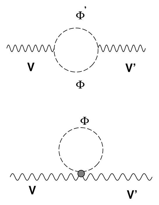
FIG. 1.: Feynman diagrams leading to leptoquark contribution to vector-boson self-energies.

FIG. 2.: Feynman diagrams leading to leptoquark contribution to the muon decay. The direction of the lines depends upon the leptoquark type.

FIG. 3.: Feynman diagrams leading to leptoquark contribution to the vertex $Zf\bar{f}$. The direction of the lines depends upon the leptoquark type.

FIG. 4.: Bounds (95% CL) on the leptoquark masses as a function of $m_{\text{top}}$ for $S_{1}$ (a), $S_{3}$ (b), and $R_{2}$ (c). The solid (dashed) lines stand for left-handed (right-handed) leptoquarks, while upper (medium, lower) lines correspond to a coupling $g_{LQ}=\sqrt{4\pi}$ ($1$, $e/s_{W}$).

TABLE I.: LEP data

$$\begin{array}[]{|l|l|}\hline\cr\hline\cr\mbox{Quantity}&\mbox{Experimental value}\\ \hline\cr M_{Z}\mbox{[GeV]}&91.1888\pm 0.0044\\ \Gamma_{Z}\mbox{[GeV]}&2.4974\pm 0.0038\\ \sigma_{\rm had}^{0}\mbox{[nb]}&41.49\pm 0.12\\ R_{e}=\frac{\Gamma({\rm had})}{\Gamma(e^{+}e^{-})}&20.850\pm 0.067\\ R_{\mu}=\frac{\Gamma({\rm had})}{\Gamma(\mu^{+}\mu^{-})}&20.824\pm 0.059\\ R_{\tau}=\frac{\Gamma({\rm had})}{\Gamma(\mu^{+}\mu^{-})}&20.749\pm 0.070\\ A_{FB}^{0e}&0.0156\pm 0.0034\\ A_{FB}^{0\mu}&0.041\pm 0.0021\\ A_{FB}^{0\tau}&0.0228\pm 0.0026\\ A_{\tau}^{0}&0.143\pm 0.010\\ A_{e}^{0}&0.135\pm 0.011\\ R_{b}=\frac{\Gamma(b\bar{b})}{\Gamma({\rm had})}&0.2202\pm 0.0020\\ R_{c}=\frac{\Gamma(c\bar{c})}{\Gamma({\rm had})}&0.1583\pm 0.0098\\ A_{FB}^{0b}&0.0967\pm 0.0038\\ A_{FB}^{0c}&0.0760\pm 0.0091\\ \hline\cr\hline\cr\end{array}$$

TABLE II.: Lower limits (95 % CL) for the mass of third generation leptoquarks in GeV for different values of the couplings, assuming $m_{\text{top}}=175$ GeV, $\alpha_{s}(M_{Z}^{2})=0.126$, and $M_{H}=300$ GeV.

g	$S_{1}^{R}$	$S_{1}^{L}$	$S_{3}$	$R_{2}^{R}$	$R_{2}^{L}$	$\tilde{S}_{1}^{R}$	$\tilde{R}_{2}^{L}$
$\sqrt{4\pi}$	4000	5000	6000	4000	5000	280	400
1	750	900	1100	850	1000	—	—
${\displaystyle\frac{e}{s_{W}}}$	350	400	600	400	500	—	—

REFERENCES

• [1] See, for instance, D. Schaile, Precision Tests of the Electroweak Interaction, plenary talk (Pl-2) presented at the 27th International Conference on High Energy Physics, Glasgow, Scotland, July 1994; “Combined Preliminary data on $Z^{0}$ Parameters from the LEP experiments and Constraints on the Standard Model”, The LEP Collaborations and The LEP Electroweak Working Group, report in preparation.
• [2] See, for instance, W. Buchmüller, Acta Phys. Austriaca Suppl. XXVII (1985) 517.
• [3] See, for instance, P. Langacker, Phys. Rep. 72 (1981) 185.
• [4] See, for instance, E. Farhi and L. Susskind, Phys. Rep. 74 (1981) 277.
• [5] See, for instance, J. L. Hewett and T. G. Rizzo, Phys. Rep. 183 (1989) 193.
• [6] L3 Collaboration, B. Adeva et al., Phys. Lett. B261 (1992) 169; OPAL Collaboration, G. Alexander et al., Phys. Lett. B263 (1992) 123; DELPHI Collaboration, P. Abreu et al., Phys. Lett. B316 (1993) 620.
• [7] CDF Collaboration, F. Abe et al., Phys. Rev. D48 (1993) 3939; D0 Collaboration, Phys. Rev. Lett. 72 (1994) 965.
• [8] ZEUS Collaboration, M. Derrick et al., Phys. Lett. B306 (1993) 173; H1 Collaboration, I. Abt et al., Nucl. Phys. B396 (1993) 3.
• [9] O. J. P. Éboli and A. V. Olinto, Phys. Rev. D38 (1988) 3461; J. L. Hewett and S. Pakvasa, ibid. D37 (1988) 3165; J. Ohnemus, S. Rudaz, T. F. Wash, and P. Zerwas, Phys. Lett. B334 (1994) 203.
• [10] W. Buchmüller, R. Rückl, and D. Wyler, Phys. Lett. B191 (1987) 442.
• [11] J. Wudka, Phys. Lett. B167 (1986) 337; M. A. Doncheski and J. L. Hewett, Z. Phys. C56 (1992) 209; J. Blümlein, F. Boos, and A. Pukhov, preprint DESY-94-072, hep-ph/9404321.
• [12] J. L. Hewett and T. G. Rizzo, Phys. Rev. D36 (1987) 3367; J. L. Hewett and S. Pakvasa Phys. Lett. B227 (1987) 178; J. E. Cieza and O. J. P. Éboli, Phys. Rev. D47 (1993) 837; J. Blümein and R. Rückl, Phys. Lett. B304 (1993) 337; J. Blümlein and E. Boos, preprint DESY-94-114, hep-ph/9408250.
• [13] O. J. P. Éboli et al., Phys. Lett. B311 (1993) 147; H. Nadeau and D. London, Phys. Rev. D47, (1993) 3742; M. A. Doncheski and S. Godfrey, University of Ottawa preprint OCIP-C-94-7, hep-ph/9407317.
• [14] G. Bélanger, D. London, and H. Nadeau, Phys. Rev. D49 (1994) 3140.
• [15] M. Leurer, Phys. Rev. Lett. 71 (1993) 1324; Phys. Rev. D49 (1994) 333.
• [16] S. Davidson, D. Bailey, and A. Campbell, Z. Phys. C61 (1994) 613.
• [17] O. Shanker, Nucl. Phys. B204 (1982) 375.
• [18] W. Buchmüller and D. Wyler, Phys. Lett. B177 (1986) 377; J. C. Pati and A. Salam, Phys. Rev. D10 (1974) 275.
• [19] P. Langacker, Phys. Lett. B256 (1991) 277; P. Langacker, M. Luo, and A. K. Mann, Rev. Mod. Phys. 64 (1992) 87.
• [20] See, for example, W. Hollik, in the Proceedings of the VII Swieca Summer School, editors O. J. P. Éboli and V. O. Rivelles (World Scientific, Singapore, 1994).
• [21] G. ’t Hooft and M. Veltman, Nucl. Phys. B44 (1972) 189; C. G. Bollini and J. J. Giambiagi, Nuovo Cim. 12B (1972) 20.
• [22] G. Passarino and M. Veltman, Nucl. Phys. B160 (1979) 151.
• [23] J. C. Ward, Phys. Rev. 78 (1950) 182; Y. Takahashi, Nuovo Cim. 6 (1957) 317; J. C. Taylor, Nucl. Phys. B33 (1971) 436; A. A. Slavnov, Theor. and Math. Phys. 10 (1972) 99.
• [24] M. E. Peskin and Takeuchi, Phys. Rev. Lett. 65 (1990) 964; G. Altarelli, R. Barbieri, and F. Caravaglios, Nucl. Phys. B405 (1993) 3.
• [25] G. Altarelli, preprint CERN-TH.7464/94.
• [26] D. Bardine et al., Z. Phys. C44 (1989) 493; Comput. Phys. Commun. 59 (1990) 303; Nucl. Phys. B351 (1991) 1; Phys. Lett. B255 (1991) 290; CERN-TH 6443/92 (May 1992).
• [27] J. Bernabeu, A. Pich, and A. Santamaria, Phys. Lett. B200 (1988) 569; Nucl. Phys. B363 (1991) 326.
• [28] G. Bhattacharyya, J. Ellis, and K. Sridhar, Phys. Lett. B336 (1994) 100.
Refer to caption