Cavendish–HEP–94/17

hep-ph/9411384

HADRONIZATION

B.R. Webber

Cavendish Laboratory, University of Cambridge,

Madingley Road, Cambridge CB3 0HE, U.K.

Abstract

Hadronization corrections to the predictions of perturbative QCD are reviewed. The existing models for the conversion of quarks and gluons into hadrons are summarized. The most successful models give a good description of the data on e⁺e^- event shapes and jet fragmentation functions, and suggest that the dominant hadronization effects have a $1/Q$ dependence on the hard process energy scale $Q$. In several cases the $1/Q$ terms can be understood in terms of a simple longitudinal phase-space model. They can also be inferred by relating non-perturbative renormalon effects to the infrared cutoff dependence of perturbative contributions.

Cavendish–HEP–94/17

hep-ph/9411384

November 1994

1 Introduction

Hadronic jet production at high energy colliders has proved to be one of the most valuable testing-grounds for quantum chromodynamics (QCD). At high energies, or more precisely at large momentum transfers, the QCD coupling ${\alpha}_{\mbox{\scriptsize{S}}}$ becomes small and perturbation theory becomes more reliable. Perturbative predictions to next-to-leading order, and to higher order in a few cases, give a good account of the broad features of jet production processes in e⁺e^-  hadron-hadron, and lepton-hadron collisions [1,2].

A serious barrier to further progress in jet physics, however, is our lack of understanding of the process of hadronization, in which the quarks and gluons of perturbative QCD are converted into the hadrons that are seen in the detectors. On general grounds, we expect that hadronization and other non-perturbative effects should give rise to power-suppressed corrections to quantities that are computable in perturbation theory. By power-suppressed, we mean corrections proportional to $1/Q^{p}$, where $Q$ is the hard process scale (the centre-of-mass energy in e⁺e^- annihilation). At present there are no solid arguments to exclude contributions with $p<2$ for observables like e⁺e^- event shapes, which are not fully inclusive with respect to final-state hadrons. Indeed, as we shall see, there are strong indications that the leading corrections are proportional to $1/Q$ in these cases. This is in contrast to deep inelastic structure functions and the total e⁺e^- hadronic cross section, where arguments based on the operator product expansion suggest that the dominant power corrections should decrease like $1/Q^{2}$ and $1/Q^{4}$ respectively [3].

The general picture of jet production and fragmentation which has developed and proved highly successful over the past decade has three fairly distinct stages [4]. First, on a scale of energy and time characterized by a large momentum transfer-squared $Q^{2}$, a hard subprocess takes place involving a small number of primary partons (quarks and/or gluons). For example, in e⁺e^- annihilation the hard subprocess would be e⁺e^- $\to q\bar{q}$ or, more rarely, e⁺e^- $\to q\bar{q}g$. Next, over a period characterized by scales $t$ such that $Q^{2}>t>t_{0}$, the primary partons develop into multi-parton cascades or showers by multiple gluon bremsstrahlung (Fig. 1). These cascades, which tend to develop along the directions of the primary partons owing to the collinear enhancements in QCD matrix elements, are the precursors of the jets that are observed experimentally. The showering cutoff scale, $t_{0}$, should be much greater than the intrinsic QCD scale $\Lambda^{2}$, but is otherwise somewhat arbitrary, being set by the requirement that a perturbative description in terms of partons should remain appropriate down to that scale.

Figure 1: Parton cascade in e⁺e^- annihilation.

After the parton shower has terminated, we are left with a set of partons with virtualities (virtual masses-squared) of the order of the cutoff scale $t_{0}$. From this point we enter the low momentum-transfer, long-distance regime in which non-perturbative effects cannot be neglected. The most important of these is hadronization, which converts the partons into the observed hadrons. As long as this stage of the process involves only small momentum transfers, presumably on a scale set by the QCD scale $\Lambda\sim 250$ MeV, it can be expected to lead to power corrections to quantities that are finite in perturbation theory, which are determined mainly by the two earlier stages of jet production and development.

At present the only detailed descriptions of the hadronization process are provided by models, which are discussed briefly in the following section. In Sect. 3, we consider the predictions of these models for hadronization corrections in e⁺e^- event shapes, where a rather clear pattern of $1/Q$ corrections emerges.

Next, in Sect. 4, we turn to a discussion of hadron energy spectra in jet fragmentation. Here hadronization enters in two distinct ways. First, the the shapes and normalizations of the spectra of the various hadronic species provide detailed tests of hadronization models. Such quantities cannot be computed from perturbation theory, because they involve the observation of individual hadrons. However, once a fragmentation spectrum has been measured at a particular hard process energy scale $Q$, then its form at any other large scale can be predicted perturbatively using the factorization properties of QCD. The only ambiguity in the prediction, apart from the effect of higher-order terms that can be computed in principle, is again due to unknown power-suppressed corrections. We review the evidence on these corrections, which are poorly understood compared with the analogous (higher-twist) terms in deep inelastic scattering.

One formal theoretical approach to power corrections that may be useful is the study of infrared renormalons, which are generated by the divergence of perturbation theory at high orders. Renormalons are associated with power-suppressed effects but it is not so clear what they have to do with the hadronization process. However, it appears likely that there is a renormalon contribution to event shapes, corresponding to a $1/Q$ correction. This is discussed in Sect. 5. Finally, in Sect. 6, some conclusions are drawn.

2 Hadronization models

One general approach to hadronization, based on the observation that perturbation theory seems to work well down to rather low scales, is the hypothesis of local parton-hadron duality [5]. Here one supposes only that the flow of momentum and quantum numbers at the hadron level tends to follow the flow established at the parton level. Thus, for example, the flavour of the quark initiating a jet should be found in a hadron near the jet axis. The extent to which the hadron flow deviates from the parton flow reflects the irreducible smearing of order $\Lambda$ due to hadron formation. Perhaps the most striking example of local parton-hadron duality is the shape of the hadron spectrum in jet fragmentation at relatively low energies, which will be discussed in Sect. 4.4.

The simplest more explicit hadronization model [6] is the longitudinal phase-space or ‘tube’ model, in which a parton (or, more realistically, a colour-connected pair of partons) produces a jet of light hadrons which occupy a tube in $(y,p_{t})$-space, where $y=\mbox{\small${{1}\over{2}}$}\log[(E+p_{z})/(E-p_{z})]$ is rapidity and $p_{t}$ is transverse momentum, both measured with respect to the direction of the initial parton. If the hadron density in this space is $\rho(p_{t})$, the energy and momentum of a tube of rapidity length $Y$ are

$$E = \int_{0}^{Y}dy\,d^{2}p_{t}\rho(p_{t})p_{t}\cosh y=\lambda\sinh Y$$

$$P = \int_{0}^{Y}dy\,d^{2}p_{t}\rho(p_{t})p_{t}\sinh y=\lambda(\cosh Y-1)\sim E-\lambda\;,$$ (1)

where $\lambda=\int d^{2}p_{t}\rho(p_{t})p_{t}$ sets the hadronization scale. Notice that the jet momentum $P$ receives a negative hadronization correction of relative order $\lambda/E=2\lambda/Q$ for a two-jet configuration of total energy $Q$. Thus one generally expects hadronization effects to scale with energy like $1/Q$.

From Eqs. (2) we expect a mean-square hadronization contribution to jet masses of

$${\left\langle M^{2}\right\rangle}_{\mbox{\scriptsize{had}}}=E^{2}-P^{2}\sim\lambda Q\;.$$ (2)

Comparing the perturbative predictions for jet masses with experiment, one finds that a hadronization correction corresponding to

$$\lambda\sim 0.5\;\mbox{GeV}$$ (3)

is required. Note that this implies a fairly large jet mass, about $7$ GeV at $Q\sim{M}_{\mbox{\scriptsize{Z}}}$, in addition to the perturbative contribution.

We shall see that the above simple model successfully describes many of the gross features of hadronization. In order to make more detailed predictions, we need a specific model for the mechanism of hadronization. Over the years, three classes of models have been developed, which we outline briefly in the following subsections.

2.1 Independent fragmentation model

The simplest scheme for generating hadron distributions from those of partons is to suppose that each parton fragments independently. The original approach of Field and Feynman [7] was designed to reproduce the limited transverse momenta and approximate scaling of energy fraction distributions observed in quark jets produced in e⁺e^- annihilation at moderate energies. The fragmenting quark is combined with an antiquark from a $q\bar{q}$ pair created out of the vacuum, to give a “first-generation” meson with energy fraction $z$. The leftover quark, with energy fraction $(1-z)$, is fragmented in the same way, and so on until the leftover energy falls below some cutoff. Scaling follows from the energy independence of the distribution assumed for $z$, which is known as the fragmentation function. The limited transverse momenta come from the relative transverse momenta of the created $q\bar{q}$ pairs, which are given a Gaussian distribution.

For gluon fragmentation, the gluon is first split into a quark-antiquark pair, either assigning all the gluon’s momentum to one or the other ($z=0$ or 1) with equal probability [8], so that the gluon behaves at a quark of random flavour, or using the $g\to q\bar{q}$ Altarelli-Parisi splitting function [9].

With about four parameters to describe the fragmentation function, the width of the transverse momentum distribution, the ratio of strange to nonstrange pair creation, and the ratio of vector to pseudoscalar meson production, the model proved quite successful in describing the broad features of two-jet and three-jet final states in e⁺e^- annihilation at moderate energies [8-10].

A weakness of the independent fragmentation scheme, as formulated above, is that the fragmentation of a parton is supposed to depend on its energy rather than its virtuality. Indeed, the fragmenting parton is usually assumed to remain on mass shell, leading to violations of momentum conservation that have to be corrected by rescaling momenta after hadronization is completed. The residual colour and flavour of the leftover parton in each jet also have to be neutralized at this stage. There are further problems when jets become close together in angle. Instead of merging smoothly together into a single jet, as would happen if their fragmentation depended on their combined effective mass, even two precisely collinear jets remain distinguishable from a single jet.

2.2 String model

The string model of hadronization [11-14] is most easily described for e⁺e^- annihilation. Neglecting for the moment the possibility of gluon bremsstrahlung, the produced quark and antiquark move out in opposite directions, losing energy to the colour field, which is supposed to collapse into a stringlike configuration between them. The string has a uniform energy per unit length, corresponding to a linear quark confining potential, which is consistent with quarkonium spectroscopy. The string breaks up into hadron-sized pieces through spontaneous $q\bar{q}$ pair production in its intense colour field.

In practice, the string fragmentation approach does not look very different from independent fragmentation for the simple quark-antiquark system. The string may be broken up starting at either the quark or the antiquark end, or both simultaneously (the breaking points have spacelike separations, so their temporal sequence is frame dependent), and it proceeds iteratively by $q\bar{q}$ pair creation, as in independent fragmentation. What one gains is a more consistent and covariant picture, together with some constraints on the fragmentation function [13], to ensure independence of whether one starts at the quark or the antiquark, and on the transverse momentum distribution [14], which is now related to the tunnelling mechanism by which $q\bar{q}$ pairs are created in the colour field of the string.

The string model becomes more distinct from independent fragmentation when gluons are present [15]. These are supposed to produce kinks on the string, each initially carrying localized energy and momentum equal to that of its parent gluon. The fragmentation of the kinked string leads to an angular distribution of hadrons in e⁺e^- three-jet final states that is different from that predicted by independent fragmentation and in better agreement with experiment [16].

For multiparton states, such as those produced by parton showering at high $Q^{2}$ (Fig. 1), there is ambiguity about how strings should be connected between the various endpoints (quarks and antiquarks) and kinks (gluons). However, to leading order in $N_{c}^{-2}$ where $N_{c}=3$ is the number of colours, it is always possible to arrange the produced partons in a planar configuration, such that each has an equal and opposite colour to that of a neighbour (both neighbours, in the case of a gluon), like the quark and antiquark in the simplest e⁺e^- final state. The natural prescription is then to stretch the string between colour-connected neighbours, so as to make colour singlet strings of minimum invariant mass. The reformulation of parton showers in terms of sequential splitting of colour dipoles [17] leads to the same rule for string connection.

2.3 Cluster model

An important property of the parton showering process is the preconfinement of colour [18]. Preconfinement implies that the pairs of colour-connected neighbouring parton discussed above have an asymptotic mass distribution that falls rapidly at high masses and is asymptotically $Q^{2}$-independent and universal. This suggests a class of cluster hadronization models, in which colour-singlet clusters of partons form after the perturbative phase of jet development and then decay into the observed hadrons.

The simplest way for colour-singlet clusters to form after the parton cascade is through non-perturbative splitting of gluons into $q\bar{q}$ pairs [19]. Neighbouring colour-connected quarks and antiquarks can then combine into singlet clusters. The resulting cluster mass spectrum is again universal and steeply falling at high masses. Its precise form is determined by the QCD scale $\Lambda$, the parton shower cutoff $t_{0}$, and to a lesser extent the gluon-splitting mechanism. Typical cluster masses are normally two or three times $\sqrt{t_{0}}$.

If a low value of the cutoff $t_{0}$ is used, of the order of 1 GeV² or less, most clusters have masses of up to a few GeV/c² and it is reasonable to treat them as superpositions of meson resonances. In a popular model [19,20], each such cluster is assumed to decay isotropically in its rest frame into a pair of hadrons, with branching ratios determined simply by density of states. The reduced phase space for cluster decay into heavy mesons and baryons is then sufficient to account fairly well for the multiplicities of the various kinds of hadrons observed in e⁺e^- final states. Furthermore, the hadronic energy and transverse momentum distributions agree well with experiment, without the introduction of any adjustable fragmentation functions. Also, the angular distribution in e⁺e^- three-jet events is successfully described, as in the string model [16], provided soft gluon coherence is taken into account in the parton shower via ordering of the opening angles of successive branchings [21-23].

An alternative approach to cluster formation and decay is to use a higher value of the cutoff $t_{0}$ and an anisotropic, multihadron decay scheme for the resulting heavy clusters [24]. Clearly, this approach lies somewhere between the low-mass cluster and string models. In practice, even with a low value of $t_{0}$ one needs to invoke some such decay scheme for the small fraction of clusters that have masses of more that an few GeV/c², for which isotropic two-body decay is an implausible hypothesis.

2.4 QCD event generators

There are three classes of programs for generating full events from parton showers, using each of the three above-mentioned hadronization models.

Because of the difficulties discussed in connection with the independent fragmentation model, one would expect it to work best for the higher-momentum hadrons in final states consisting of a few well-separated jets. Probably on account of its simplicity, it was initially the model used most widely in conjunction with initial- and final-state parton showering for the simulation of hard hadron-hadron collisions, in the programs ISAJET [25], COJETS [26] and FIELDAJET [27].

The string hadronization model outlined above, with many further refinements, is the basis of the JETSET simulation program [28], which also includes final-state parton showering with optional angular ordering. This program gives a very good detailed description of hadronic final states in e⁺e^- annihilation up to the highest energies studied so far [29].

The JETSET hadronization scheme is also used, in combination with initial- and final-state parton cascades, in the other very successful Lund simulation programs PYTHIA [30] for hadron-hadron and LEPTO [31] for lepton-hadron collisions. The alternative formulation of parton showers in terms of colour dipole splitting mentioned above is implemented in the program ARIADNE [32], which also uses JETSET for hadronization.

The program HERWIG [33] uses a low-mass cluster hadronization model [20] in conjunction with initial- and final-state parton cascades to simulate a wide variety of hard scattering processes. The showering algorithm includes angular ordering and azimuthal correlations due to coherence and gluon polarization. This approach gives a good account of diverse data with relatively few adjustable parameters [29].

More detailed descriptions and comparisons of event generators for e⁺e^- physics may be found in Ref. [34].

3 Event shapes

A popular way to study the jet-like characteristics of hadronic final states in e⁺e^- annihilation is to use event shape variables. The procedure is to define a quantity $X$ which measures some particular aspect of the shape of the hadronic final states, for example whether the distribution of hadrons is pencil-like, planar, spherical etc. The differential cross section $d\sigma/dX$ can be measured and compared with the theoretical prediction. For the latter to be calculable in perturbation theory, the variable should be infrared safe, i.e. insensitive to the emission of soft or collinear particles. This is because the QCD matrix elements have singularities whenever a soft gluon or collinear pair of massless partons is emitted. In particular, if ${\mbox{\boldmath$p$}}_{i}$ is any 3-momentum occurring in its definition, $X$ must be invariant under the branching

$${\mbox{\boldmath$p$}}_{i}\to{\mbox{\boldmath$p$}}_{j}+{\mbox{\boldmath$p$}}_{k}$$ (4)

whenever ${\mbox{\boldmath$p$}}_{j}$ and ${\mbox{\boldmath$p$}}_{k}$ are parallel or one of them goes to zero. Quantities made out of linear sums of momenta meet this requirement. The most widely-used example is the thrust [35]

$$T=\max\,{\sum_{i}|{\mbox{\boldmath$p$}}_{i}\cdot{\mbox{\boldmath$n$}}|\over\sum_{i}|{\mbox{\boldmath$p$}}_{i}|}\;,$$ (5)

where ${\mbox{\boldmath$p$}}_{i}$ are the final-state hadron (or parton) momenta and $n$ is an arbitrary unit vector. If the ${\mbox{\boldmath$p$}}_{i}$ form an almost collinear pair of jets, then after the specified maximization or minimization $n$ will lie along the jets, defining the thrust axis of the event. As the jets become more pencil-like, the thrust approaches unity.

A event shape variable that does not require finding an event axis is the C-parameter [36]

$$C={3\over 2}\;{{\sum_{i,j}|{\mbox{\boldmath$p$}}_{i}|\,|{\mbox{\boldmath$p$}}_{j}|\,\sin^{2}\theta_{ij}}\over{(\sum_{i}|{\mbox{\boldmath$p$}}_{i}|)^{2}}}\;.$$ (6)

In the case of a pencil-like two-jet event, the $C$-parameter is close to zero; the normalization is such that the maximum value of $C$ is unity.

As mentioned in Sect. 2.4, the QCD Monte Carlo event generator programs HERWIG and JETSET are quite successful in describing the properties of e⁺e^- final states, including the distributions of event shape variables [29]. From these successes, we can hope that the models built into those programs provide some guidance on the broad features of the hadronization process. What the programs suggest is that corrections to event shapes are still substantial at energy scales $Q\sim{M}_{\mbox{\scriptsize{Z}}}$, typically around 10% of the leading-order QCD predictions. This is comparable with the next-to-leading ${\cal O}({\alpha}_{\mbox{\scriptsize{S}}}^{2})$ terms. Furthermore hadronization effects fall off rather slowly with increasing energy, apparently like $1/Q$. Thus it is imperative to understand hadronization better in order to reap the benefit of any future ${\cal O}({\alpha}_{\mbox{\scriptsize{S}}}^{3})$ calculations of event shapes.

We saw in Sect. 2 that $1/Q$ corrections are in fact generated by the simplest ‘tube’ model of hadronization. Consider for example the thrust distribution. The thrust of a two-jet event is precisely the jet momentum divided by the jet energy, and therefore in the tube model we expect a hadronization correction of $-2\lambda/Q$. Thus for $\lambda\sim 500$ MeV the hadronization correction to the thrust is expected to be

$${\left\langle\delta T\right\rangle}_{\mbox{\scriptsize{had}}}\sim-{{1\;\mbox{GeV}}\over{Q}}\;.$$ (7)

The purely perturbative prediction for the mean thrust is [38]

$$\left\langle 1-T\right\rangle=0.335{\alpha}_{\mbox{\scriptsize{S}}}+1.02{\alpha}_{\mbox{\scriptsize{S}}}^{2}+{\cal O}({\alpha}_{\mbox{\scriptsize{S}}}^{3})\;,$$ (8)

which implies that $\left\langle 1-T\right\rangle\sim 0.055$ at $Q=M_{Z}$, assuming ${\alpha}_{\mbox{\scriptsize{S}}}({M}_{\mbox{\scriptsize{Z}}})\sim 0.12$. In fact, the value measured at LEP is $\left\langle 1-T\right\rangle=0.068\pm 0.003$, consistent with an additional non-perturbative contribution of (1 GeV)$/Q$, which also agrees with the energy dependence of $\left\langle 1-T\right\rangle$ down to about $Q=15$ GeV (Fig. 2).

Figure 2: Mean value of 1 – thrust in e⁺e^- annihilation.

For the mean value of the $C$-parameter (6), the tube model predicts a hadronization correction of $3\pi\lambda/Q$, giving

$${\left\langle\delta C\right\rangle}_{\mbox{\scriptsize{had}}}\sim{{5\;\mbox{GeV}}\over{Q}}\;.$$ (9)

The perturbative prediction is

$$\left\langle C\right\rangle=1.374{\alpha}_{\mbox{\scriptsize{S}}}+4.00{\alpha}_{\mbox{\scriptsize{S}}}^{2}+{\cal O}({\alpha}_{\mbox{\scriptsize{S}}}^{3})\;,$$ (10)

which implies $\left\langle C\right\rangle\sim 0.222$ at $Q=M_{Z}$, again assuming ${\alpha}_{\mbox{\scriptsize{S}}}({M}_{\mbox{\scriptsize{Z}}})\sim 0.12$. The value measured at LEP is $\left\langle C\right\rangle=0.260\pm 0.006$, which is consistent with the expected additional non-perturbative contribution, although in this case there are no published lower-energy measurements with which to check the $Q$-dependence.

Turning to the differential distributions of event shape variables, hadronization seems mainly to cause a smearing by an amount proportional to $1/Q$. The effect is therefore most pronounced in the neighbourhood of the peak of the distribution, as shown for the thrust distribution in Fig. 3. The shaded band shows the variation in the hadronization corrections deduced from JETSET and HERWIG, where the correction is defined as the ratio of the parton- and hadron-level Monte Carlo predictions. The predominant effect of hadronization is to smear out the parton-level peak at low values of $1-T$, enhancing the hadron-level distribution at intermediate values of the thrust.

Figure 3: Thrust distribution in Z⁰ $\to$ hadrons, with detector and hadronization corrections.

4 Jet fragmentation

We have illustrated in Sect. 3 the use of perturbation theory to calculate ‘infrared safe’ quantities such as e⁺e^- event shapes. There are in addition predictions that can be made concerning some quantities that are ‘infrared sensitive’, i.e. that have infrared and collinear singularities in perturbation theory. Such quantities can still be handled provided the singularities can be collected into an overall factor which describes the sensitivity of the quantity to long-distance physics. The divergence of this factor corresponds to the fact that long-distance phenomena are not reliably predicted by perturbation theory. Therefore the divergent factor must be replaced by a finite factor determined either by experiment or according to some non-perturbative model. Once this is done, perturbation theory can be used to predict the scale dependence of the quantity.

The best known example of a perturbative prediction concerning a factorizable infrared-sensitive quantity is the phenomenon of scaling violation in hadron structure functions. There one studies the parton distributions inside a hadron, probed by deep inelastic lepton scattering. Here we consider the related phenomenon for the fragmentation of a jet, produced for example in e⁺e^- annihilation, into hadrons of a given type $h$.

4.1 Fragmentation functions

The total fragmentation function for hadrons of type $h$ in e⁺e^- annihilation at c.m. energy $\sqrt{s}$ as is defined as

$$F^{h}(x,s)={{1}\over{{\sigma}_{\mbox{\scriptsize{tot}}}}}{{d\sigma}\over{dx}}(e^{+}e^{-}\to hX)$$ (11)

where $x=2E_{h}/\sqrt{s}\leq 1$ is the scaled hadron energy. These functions are predicted by the QCD event generators discussed in Sect. 2.4, and experimental data for the various identifiable hadron species provide strong constraints on the hadronization models used in the programs. Generally speaking, the most developed event generators, JETSET and HERWIG, give fairly good agreement with experiment, although there are problems with the yields of heavy strange particles [29].

The fragmentation function (11) can be represented as a sum of contributions from the different primary partons $i=u,d,\ldots,g$:

$$F^{h}(x,s)=\sum_{i}\int{{dz}\over{z}}C_{i}(s;z,{\alpha}_{\mbox{\scriptsize{S}}})D^{h}_{i}(x/z,s)\;.$$ (12)

In lowest order the coefficient function $C_{g}$ for gluons is zero, while for quarks $C_{i}=g_{i}(s)\delta(1-z)$ where $g_{i}(s)$ is the appropriate electroweak coupling.

We cannot compute the parton $\to$ hadron fragmentation functions $D^{h}_{i}$ from perturbation theory, since the production of hadrons is not a perturbative process. We might consider trying to compute functions $D^{j}_{i}$ that would describe the fragmentation of partons of type $i$ into partons of type $j$. However, they would be infinite, since the probability of emitting a collinear gluon or light quark is divergent. Nevertheless, it can be shown [37] that all such divergences are factorizable in the sense that one can write

$$D^{j}_{i}(x,t)=\sum_{k}\int_{x}^{1}dz\,K^{k}_{i}(z,t,t_{0})\,D^{j}_{k}(x/z,t_{0})$$ (13)

where the kernel function $K^{k}_{i}$ is perturbatively calculable and $K^{k}_{i}(z,t,t)=\delta_{ik}\,\delta(1-z)$.

In the real world, hadrons are formed and fragmentation functions are not divergent. As long as the scales $t$ and $t_{0}$ are large, we would not expect the form of Eq. (13) to be affected by such long-distance phenomena. Therefore we replace $j$ by $h$ and apply the equation to hadronic fragmentation functions. After measuring these functions at some scale $t_{0}$, we can use the equation to predict their form at any other scale $t$, as long as both $t$ and $t_{0}$ are large enough for perturbation theory to be applicable in the calculation of the kernel $K^{k}_{i}$.

4.2 Scaling violation in jet fragmentation

Consider the change in a fragmentation function $D_{i}(x,t)$ when the hard process scale is increased from $t$ to $t+dt$. Such a change can only occur via the splitting of a parton of type $i$ in this scale interval. Hence the fragmentation functions $D_{i}$ satisfy evolution equations of the Altarelli-Parisi type, first introduced for deep inelastic scattering [39]:

$$t{{\partial}\over{\partial t}}D_{i}(x,t)=\sum_{j}\int{{dz}\over{z}}{{{\alpha}_{\mbox{\scriptsize{S}}}}\over{2\pi}}P_{ji}(z,{\alpha}_{\mbox{\scriptsize{S}}})D_{j}(x/z,t)\;.$$ (14)

The $i\to j$ parton splitting function $P_{ji}$ has a perturbative expansion of the form

$$P_{ji}(z,{\alpha}_{\mbox{\scriptsize{S}}})=P^{(0)}_{ji}(z)+{{{\alpha}_{\mbox{\scriptsize{S}}}}\over{2\pi}}P^{(1)}_{ji}(z)+\cdots$$ (15)

where the lowest-order splitting function $P^{(0)}_{ji}(z)$ is the same in fragmentation and deep inelastic scattering but the higher-order terms are different. The effect of splitting is qualitatively the same in both cases: as the scale increases, one observes a scaling violation in which the $x$ distribution is shifted towards lower values.

The most common strategy for solving the evolution equations (14) is to take moments (Mellin transforms) with respect to $x$:

$$\tilde{D}(N,t)=\int_{0}^{1}dx\;x^{N-1}\;D(x,t)\;,$$ (16)

the inverse Mellin transform being

$$D(x,t)={{1}\over{2\pi i}}\int_{C}dN\;x^{-N}\;\tilde{D}(N,t)\;,$$ (17)

where the integration contour $C$ in the complex $N$ plane is parallel to the imaginary axis and to the right of all singularities of the integrand. After Mellin transformation, the convolution on the right-hand side of Eq. (14) becomes simply a product.

The moments $\tilde{P}_{ji}$ of the splitting functions are called anomalous dimensions, usually denoted by $\gamma_{ji}(N,{\alpha}_{\mbox{\scriptsize{S}}})$. In lowest order they take the form

$$\gamma^{(0)}_{qq}(N) = C_{F}\Bigg{[}-{{1}\over{2}}+{{1}\over{N(N+1)}}-2\sum^{N}_{k=2}{{1}\over{k}}\Bigg{]}$$

$$\gamma^{(0)}_{qg}(N) = T_{R}\Bigg{[}{{(2+N+N^{2})}\over{N(N+1)(N+2)}}\Bigg{]}$$

$$\gamma^{(0)}_{gq}(N) = C_{F}\Bigg{[}{{(2+N+N^{2})}\over{N(N^{2}-1)}}\Bigg{]}$$ (18)

$$\gamma^{(0)}_{gg}(N) = 2C_{A}\Bigg{[}-{{1}\over{12}}+{{1}\over{N(N-1)}}+{{1}\over{(N+1)(N+2)}}-\sum_{k=2}^{N}{{1}\over{k}}\Bigg{]}-{{2}\over{3}}N_{f}T_{R}\;,$$

where the QCD colour factors are $C_{F}=\mbox{\small${{4}\over{3}}$}$, $C_{A}=3$, $T_{R}=\mbox{\small${{1}\over{2}}$}$, and $N_{f}$ is the number of quark flavours with masses less than the relevant scale $\sqrt{t}$.

We can consider fragmentation function combinations which are non-singlet in flavour space, such as $D_{V}=D_{q_{i}}-D_{\bar{q}_{i}}$ or $D_{q_{i}}-D_{q_{j}}$. In these combinations the mixing with the flavour singlet gluons drops out and for a fixed value of ${\alpha}_{\mbox{\scriptsize{S}}}$ the solution is simply

$$\tilde{D}_{V}(N,t)=\tilde{D}_{V}(N,t_{0})\left({{t}\over{t_{0}}}\right)^{\gamma_{qq}(N,{\alpha}_{\mbox{\scriptsize{S}}})}\;.$$ (19)

For a running coupling ${\alpha}_{\mbox{\scriptsize{S}}}(t)$, the scaling violation is no longer power-behaved in $t$. Inserting the lowest-order form for the running coupling,

$${\alpha}_{\mbox{\scriptsize{S}}}(t)={{1}\over{b\ln(t/\Lambda^{2})}}$$ (20)

where $b=(11C_{A}-2N_{f})/12\pi$, we find the solution

$$\tilde{D}_{V}(N,t)=\tilde{D}_{V}(N,t_{0})\left({{{\alpha}_{\mbox{\scriptsize{S}}}(t_{0})}\over{{\alpha}_{\mbox{\scriptsize{S}}}(t)}}\right)^{d_{qq}(N)},\;\;d_{qq}(N)={{\gamma^{(0)}_{qq}(N)}\over{2\pi b}}\;,$$ (21)

which varies like a power of $\ln t$.

For the singlet quark fragmentation function

$$D_{S}=\sum_{i}(D_{q_{i}}+D_{\bar{q}_{i}})\;,$$ (22)

we have mixing with the fragmentation of the gluon and the evolution equation becomes a matrix relation of the form

$$t{{\partial}\over{\partial t}}\left(\begin{array}[]{c}\tilde{D}_{S}\\ \tilde{D}_{g}\end{array}\right)=\left(\begin{array}[]{cc}\gamma_{qq}&2N_{f}\gamma_{gq}\\ \gamma_{qg}&\gamma_{gg}\end{array}\right)\left(\begin{array}[]{c}\tilde{D}_{S}\\ \tilde{D}_{g}\end{array}\right)\;.$$ (23)

The anomalous dimension matrix in this equation has two real eigenvalues $\gamma_{\pm}$ given by

$$\gamma_{\pm}=\mbox{\small${{1}\over{2}}$}[\gamma_{gg}+\gamma_{qq}\pm\sqrt{(\gamma_{gg}-\gamma_{qq})^{2}+8N_{f}\gamma_{gq}\gamma_{qg}}]\;.$$ (24)

Expressing $D_{S}$ and $D_{g}$ as linear combinations of the corresponding eigenvectors $D_{+}$ and $D_{-}$, we find that they evolve as superpositions of terms of the form (21) with $\gamma_{+}$ and $\gamma_{-}$ in the place of $\gamma_{qq}$.

At small $x$, corresponding to $N\to 1$, the $g\to g$ anomalous dimension becomes dominant and we find $\gamma_{+}\to\gamma_{gg}\to\infty$, $\gamma_{-}\to\gamma_{qq}\to 0$. This region requires special treatment, as we discuss in the following two sections.

There are several complications in the experimental study of scaling violation in jet fragmentation [40]. First, the energy dependence of the electroweak couplings $g_{i}(s)$ that enter into Eq. (12) is especially strong in the energy region presently under study ($\sqrt{s}=20-90$ GeV). In particular, the $b$-quark contribution more than doubles in this range. The fragmentation of the $b$ quark into charged hadrons, including the decay products of the $b$-flavoured hadron, is expected to be substantially softer than that of the other quarks, so its increased contribution can give rise to a ‘fake’ scaling violation that has nothing to do with QCD. A smaller, partially compensating effect is expected in charm fragmentation. These effects can be eliminated by extracting the $b$ and $c$ fragmentation functions at $\sqrt{s}={M}_{\mbox{\scriptsize{Z}}}$ from tagged heavy quark events, and evolving them separately to other energies.

Secondly, one requires the gluon fragmentation function $D_{g}(x,s)$ in addition to those of the quarks. Although the gluon does not couple directly to the electroweak current, it contributes in higher order, and mixes with the quarks through evolution. Its fragmentation can be studied in tagged heavy-quark three-jet ($Q\bar{Q}g$) events, or via the longitudinal fragmentation function (see Sect. 4.5).

A final complication is that power corrections to fragmentation functions, of the form $f(x)/Q^{p}$, are not well understood. As in the case of event shapes, Monte Carlo studies [40] suggest that hadronization can lead to $1/Q$ corrections. Therefore, possible contributions of this form should be included in the parametrization when fitting the scaling violation.

Preliminary results of an analysis of scaling violation in the charged hadron spectrum by the ALEPH collaboration [41], based on a comparison of LEP data with those from lower-energy experiments, are shown in Fig. 4. Also included are their separate fragmentation functions for light ($u,d,s$) quarks, $b$ quarks and gluons, showing that the latter two functions are significantly softer (quite similar to each other, within the errors) at $\sqrt{s}={M}_{\mbox{\scriptsize{Z}}}$. An overall fit in the range $22\leq\sqrt{s}\leq 91.2$ GeV, $0.1<x<0.8$, incorporating full next-to-leading-order evolution and a simple parametrization of $1/Q$ power corrections, gives a good description of the data in the fitted region, as shown by the curves. The fitted power corrections are small and the value obtained for ${\alpha}_{\mbox{\scriptsize{S}}}({M}_{\mbox{\scriptsize{Z}}})$ ($0.127\pm 0.011$) is not highly sensitive to the form assumed for them. Indeed, a $1/Q^{2}$ dependence is not ruled out, and it may be that in this case the Monte Carlo models are misleading and $1/Q$ corrections are in fact absent. An operator-product approach to fragmentation, developed in Ref. [42], does indeed suggest that 1/Q corrections are absent.

Figure 4: Scaling violation in e⁺e^- fragmentation functions.

4.3 Average multiplicity

The average number of hadrons of type $h$ in a jet initiated by a parton $i$ at scale $t$, ${\cal N}^{h}_{i}(t)$, is just the integral of the fragmentation function, which is the $N=1$ moment in the notation of Eq. (16):

$${\cal N}^{h}_{i}(t)=\int_{0}^{1}dx\,D^{h}_{i}(x,t)=\tilde{D}^{h}_{i}(1,t)\;.$$ (25)

If we try to compute the $t$ dependence of this quantity, we immediately encounter the problem that the anomalous dimensions $\gamma_{gq}$ and $\gamma_{gg}$ given in Eq. (4.2) have poles at $N=1$. The reason is that for $N\leq 1$ the moment integrals are dominated by the region of small $z$, where $P_{gi}(z)$ has a divergence associated with soft gluon emission.

In fact, however, we can still solve the evolution equation for the average multiplicity provided we take into account the suppression of soft gluon emission due to QCD coherence [22,23]. The leading effect of coherence is obtained simply by changing the evolution variable from virtual mass-squared to the quantity $t=E^{2}[1-\cos\theta]$, where $\theta$ is the opening angle, and imposing angular ordering, $\theta^{\prime}<\theta$ [22,43]. Thus in terms of the newly-defined evolution variable the ordering condition is $t^{\prime}<z^{2}t$ and Eq. (14) becomes

$$t{{\partial}\over{\partial t}}D_{i}(x,t)=\sum_{j}\int_{x}^{1}{{dz}\over{z}}{{{\alpha}_{\mbox{\scriptsize{S}}}}\over{2\pi}}P_{ji}(z,{\alpha}_{\mbox{\scriptsize{S}}})D_{j}(x/z,z^{2}t)\;.$$ (26)

Notice that this differs from the conventional Altarelli-Parisi equation only in the $z$-dependent change of scale on the right-hand side. This change is not important for most values of $x$ but we shall see that it is crucial at small $x$.

For simplicity, consider first the solution of Eq. (26) taking ${\alpha}_{\mbox{\scriptsize{S}}}$ fixed and neglecting the sum over different branchings. Then taking moments as usual we have

$$t{{\partial}\over{\partial t}}\tilde{D}(N,t)={{{\alpha}_{\mbox{\scriptsize{S}}}}\over{2\pi}}\int_{x}^{1}dz\,z^{N-1}P(z)\tilde{D}(N,z^{2}t)\;.$$ (27)

Now if we try a solution of the form

$$\tilde{D}(N,t)\propto t^{\gamma(N,{\alpha}_{\mbox{\scriptsize{S}}})}$$ (28)

we find that the anomalous dimension $\gamma(N,{\alpha}_{\mbox{\scriptsize{S}}})$ must satisfy the implicit equation

$$\gamma(N,{\alpha}_{\mbox{\scriptsize{S}}})={{{\alpha}_{\mbox{\scriptsize{S}}}}\over{2\pi}}\int_{0}^{1}dz\,z^{N-1+2\gamma(N,{\alpha}_{\mbox{\scriptsize{S}}})}P(z)\;.$$ (29)

When $N-1$ is not small, we may neglect the $2\gamma(N,{\alpha}_{\mbox{\scriptsize{S}}})$ in the exponent of Eq. (29) and then we obtain the usual explicit formula for the anomalous dimension. For $N\simeq 1$, the region we are interested in, the $z\to 0$ behaviour of $P(z)$ dominates and we may as a first approximation keep only those terms that are singular at $z=0$. The most important such term appears in the gluon-gluon splitting function: $P_{gg}(z)\to 2C_{A}/z$ as $z\to 0$. Then Eq. (29) implies that near $N=1$

$$\gamma_{gg}(N,{\alpha}_{\mbox{\scriptsize{S}}})={{C_{A}{\alpha}_{\mbox{\scriptsize{S}}}}\over{\pi}}{{1}\over{N-1+2\gamma_{gg}(N,{\alpha}_{\mbox{\scriptsize{S}}})}}\;,$$ (30)

and hence

$$\gamma_{gg}(N,{\alpha}_{\mbox{\scriptsize{S}}})\;=\;{{1}\over{4}}\left[\sqrt{(N-1)^{2}+{{8C_{A}{\alpha}_{\mbox{\scriptsize{S}}}}\over{\pi}}}-(N-1)\right]$$

$$=\sqrt{{{C_{A}{\alpha}_{\mbox{\scriptsize{S}}}}\over{2\pi}}}-{{1}\over{4}}(N-1)+{{1}\over{32}}\sqrt{{{2\pi}\over{C_{A}{\alpha}_{\mbox{\scriptsize{S}}}}}}(N-1)^{2}+\cdots\;.$$ (31)

Thus for $N\to 1$ the gluon-gluon anomalous dimension behaves like the square root of ${\alpha}_{\mbox{\scriptsize{S}}}$. How can this behaviour emerge from perturbation theory, which deals only in integer powers of ${\alpha}_{\mbox{\scriptsize{S}}}$? The answer is that at any fixed $N\neq 1$ we can expand Eq. (4.3) in a different way for sufficiently small ${\alpha}_{\mbox{\scriptsize{S}}}$:

$$\gamma_{gg}(N,{\alpha}_{\mbox{\scriptsize{S}}})={{C_{A}{\alpha}_{\mbox{\scriptsize{S}}}}\over{\pi(N-1)}}-2\left({{C_{A}{\alpha}_{\mbox{\scriptsize{S}}}}\over{\pi}}\right)^{2}{{1}\over{(N-1)^{3}}}+\cdots\;.$$ (32)

This series displays the terms that are most singular as $N\to 1$ in each order. These terms have been resummed in the expression (4.3), allowing the perturbation series to be analytically continued outside its circle of convergence $|{\alpha}_{\mbox{\scriptsize{S}}}|<(\pi/8C_{A})|N-1|^{2}$. By definition, the behaviour outside this circle (in particular, for the average multiplicity, at $N=1$) cannot be represented by the series any more, even though it is fully implied by it.

At sufficiently small $x$, the $N\to 1$ singularity of the gluon-gluon anomalous dimension dominates in all fragmentation functions. Thus we obtain the behaviour (28) with $\gamma=\gamma_{gg}$ for the total fragmentation function defined in Eq. (12). To predict this behaviour quantitatively we need to take account of the running of ${\alpha}_{\mbox{\scriptsize{S}}}$, which can be done in the same way as for the other moments. Writing Eq. (28) in the form

$$\tilde{F}(N,t)\sim\tilde{D}(N,t)\propto\exp\left[\int^{t}\gamma_{gg}(N,{\alpha}_{\mbox{\scriptsize{S}}}){{dt^{\prime}}\over{t^{\prime}}}\right]\;,$$ (33)

we have to replace $\gamma_{gg}(N,{\alpha}_{\mbox{\scriptsize{S}}})$ in the integrand by $\gamma_{gg}(N,{\alpha}_{\mbox{\scriptsize{S}}}(t^{\prime}))$. We then write

$$\int^{t}\gamma_{gg}(N,{\alpha}_{\mbox{\scriptsize{S}}}(t^{\prime})){{dt^{\prime}}\over{t^{\prime}}}=\int^{{\alpha}_{\mbox{\scriptsize{S}}}(t)}{{\gamma_{gg}(N,{\alpha}_{\mbox{\scriptsize{S}}})}\over{\beta({\alpha}_{\mbox{\scriptsize{S}}})}}\,d{\alpha}_{\mbox{\scriptsize{S}}}\;,$$ (34)

where $\beta({\alpha}_{\mbox{\scriptsize{S}}})=-b{\alpha}_{\mbox{\scriptsize{S}}}^{2}+\cdots$, and find

$$\tilde{F}(N,t) \sim \exp\Biggl{[}{{1}\over{b}}\sqrt{{{2C_{A}}\over{\pi{\alpha}_{\mbox{\scriptsize{S}}}}}}-{{1}\over{4b{\alpha}_{\mbox{\scriptsize{S}}}}}(N-1)$$ (35)

$$+ {{1}\over{48b}}\sqrt{{{2\pi}\over{C_{A}{\alpha}_{\mbox{\scriptsize{S}}}^{3}}}}(N-1)^{2}+\cdots\Biggr{]}_{{\alpha}_{\mbox{\scriptsize{S}}}={\alpha}_{\mbox{\scriptsize{S}}}(t)}\;.$$

In e⁺e^- annihilation the scale $t$ (the upper limit on $E^{2}[1-\cos\theta]$ for any branching) is of the order of the centre-of-mass energy-squared $s$, and so the average multiplicity of any hadronic species has the asymptotic behaviour

$$\left\langle n(s)\right\rangle=\tilde{F}(1,s)\sim\exp{{1}\over{b}}\sqrt{{{2C_{A}}\over{\pi{\alpha}_{\mbox{\scriptsize{S}}}(s)}}}\sim\exp\sqrt{{{2C_{A}}\over{\pi b}}\ln\left({{s}\over{\Lambda^{2}}}\right)}\;.$$ (36)

If the next-to-leading singularities of the anomalous dimensions, i.e. the terms with one less power of $1/(N-1)$ in Eq. (32), are also resummed, the expression (36) is multiplied by a power of ${\alpha}_{\mbox{\scriptsize{S}}}(s)$ [44]. The resulting prediction, shown by the solid curve in Fig. 5, is in very good agreement with experiment [45].

Figure 5: Average multiplicity of charged hadrons in e⁺e^- annihilation.

4.4 Small-$x$ fragmentation

The behaviour of $\tilde{F}(N,s)$ away from $N=1$ determines the form of small-$x$ fragmentation functions via the inverse Mellin transformation (17). Keeping the first three terms in the Taylor expansion of the exponent, as displayed in Eq. (35), gives a simple Gaussian function of $N$ which transforms into a Gaussian in the variable $\xi\equiv\ln(1/x)$:

$$xF(x,s)\propto\exp\left[-{{1}\over{2\sigma^{2}}}(\xi-\xi_{p})^{2}\right]\;,$$ (37)

where the peak position is

$$\xi_{p}={{1}\over{4b{\alpha}_{\mbox{\scriptsize{S}}}(s)}}\sim{{1}\over{4}}\ln s$$ (38)

and the width of the distribution of $\xi$ is

$$\sigma=\left({{1}\over{24b}}\sqrt{{{2\pi}\over{C_{A}{\alpha}_{\mbox{\scriptsize{S}}}^{3}(s)}}}\right)^{{{1}\over{2}}}\propto(\ln s)^{{{3}\over{4}}}\;.$$ (39)

Again, one can compute next-to-leading corrections to these predictions [46], and the results agree very well with the form and energy dependence of fragmentation functions at small $x$ as measured in e⁺e^- annihilation (Fig. 6) [47]. This provides support for the notion of local parton-hadron duality mentioned in Sect. 2. We assumed in Eq. (33) that the $N$-dependence of the Mellin-transformed fragmentation function is dominated by the perturbative part involving the anomalous dimension, and that the non-perturbative factor is relatively smooth. Smoothness in $N$ transforms into locality in $x$. Although the violation of scaling ensures that this is valid asymptotically, it seems to be a good approximation already at energies as low as 14 GeV.

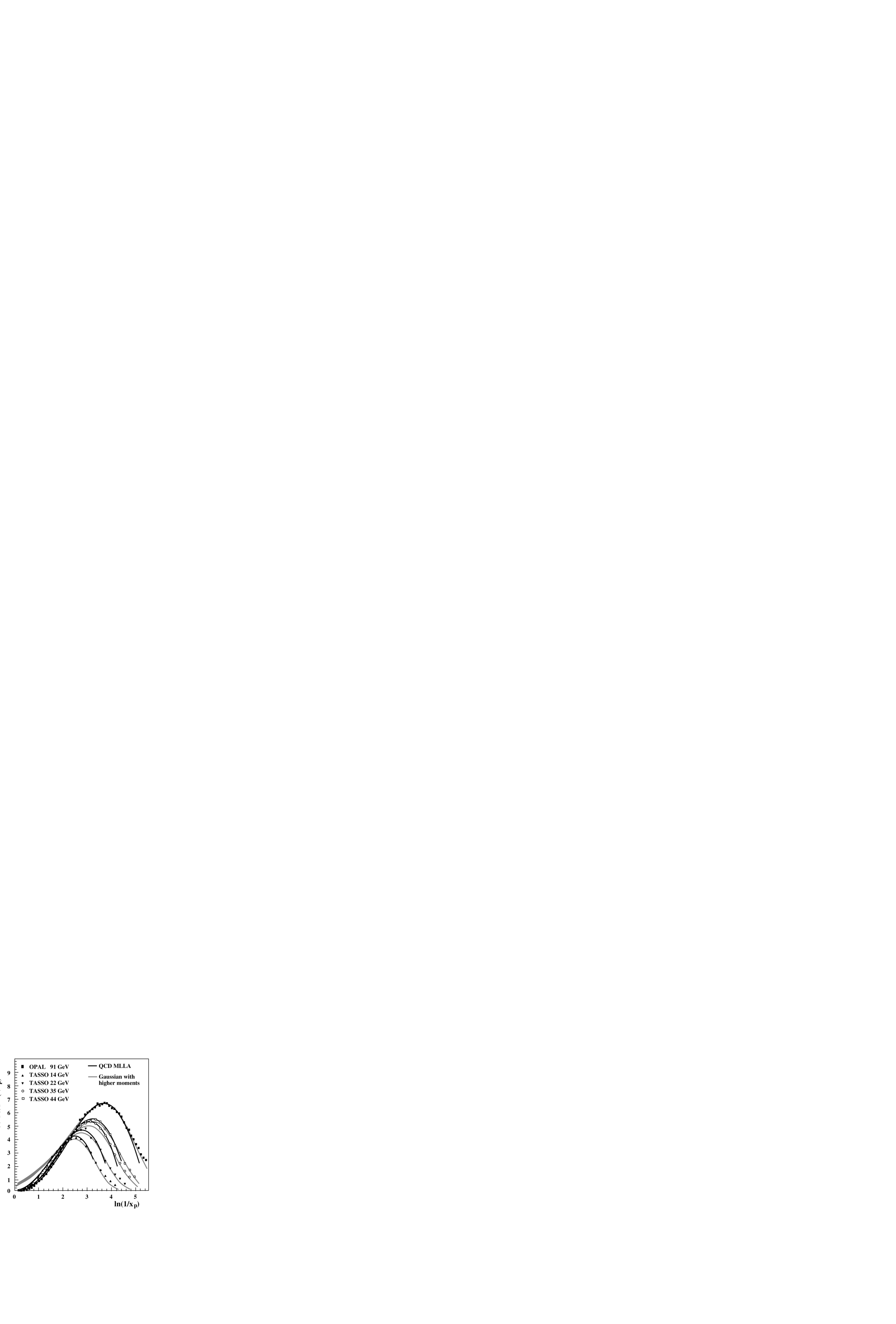
Figure 6: Distribution of $\xi=\ln(1/x)$ in e⁺e^- annihilation.

The energy-dependence (38) of the peak in the $\xi$-distribution is also a striking illustration of soft gluon coherence, which is the origin of the suppression of hadron production at small $x$. Of course, a decrease at very small $x$ is expected on purely kinematical grounds, but this would occur at particle energies proportional to their masses, i.e. at $x\propto m/\sqrt{s}$ and hence $\xi\sim{{1}\over{2}}\ln s$. Thus if the suppression were purely kinematic the peak position $\xi_{p}$ would vary twice as rapidly with energy, which is ruled out by the data (Fig. 7).

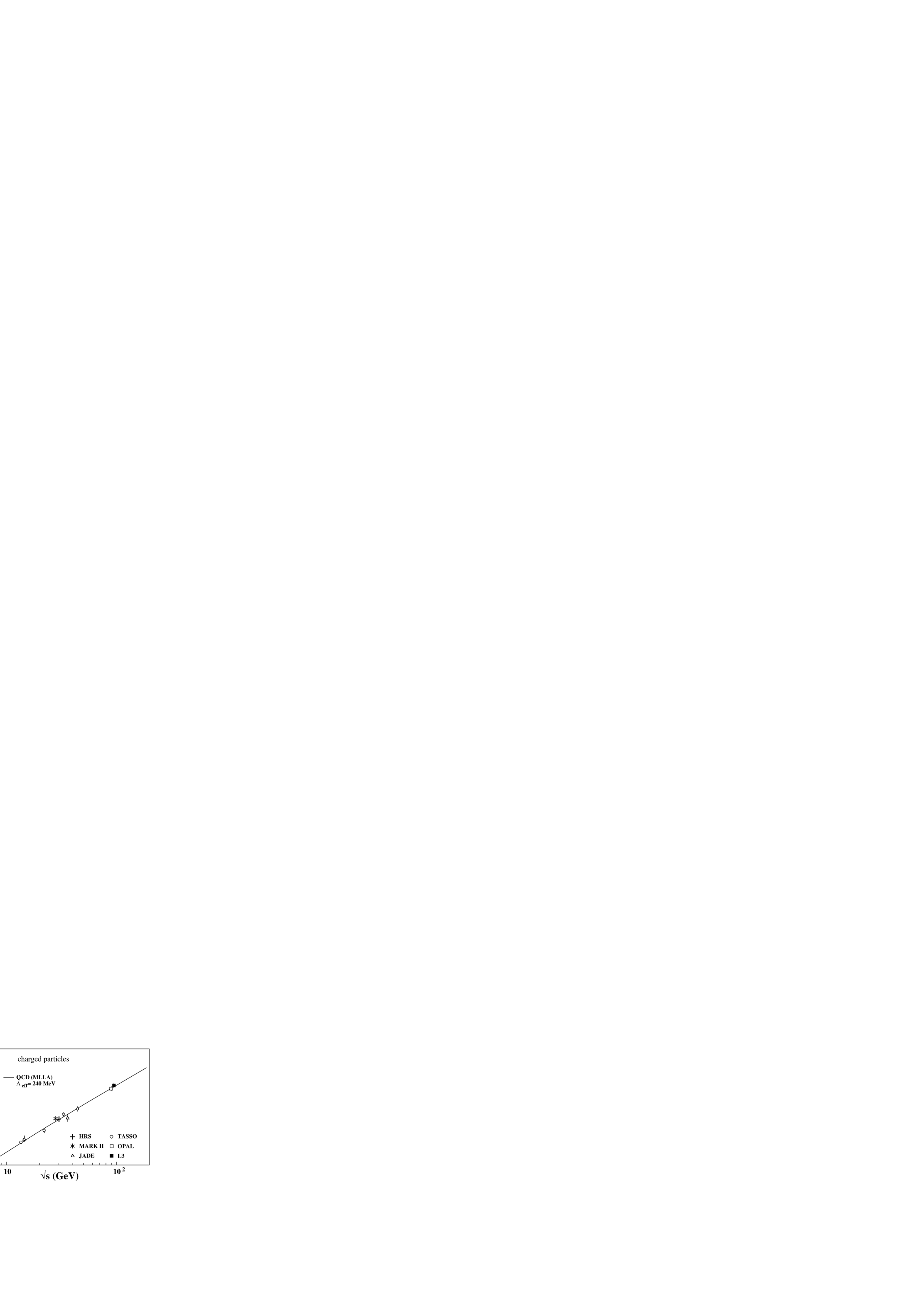
Figure 7: Position of the peak in the $\xi$-distribution.

4.5 Longitudinal fragmentation

Recently, the ALEPH [41] and OPAL [48] collaborations at LEP have presented preliminary results of the first analyses of the longitudinal fragmentation function in e⁺e^- annihilation. This is defined in terms of the joint distribution in the energy fraction $x$ and the angle $\theta$ between the observed hadron and the incoming electron beam [40]:

$${{1}\over{{\sigma}_{\mbox{\scriptsize{tot}}}}}{{d^{2}\sigma}\over{dx\,d\cos\theta}}={{3}\over{8}}(1+\cos^{2}\theta)\,{F}_{\mbox{\scriptsize{T}}}(x)+{{3}\over{4}}\sin^{2}\theta\,{F}_{\mbox{\scriptsize{L}}}(x)+{{3}\over{4}}\cos\theta\,{F}_{\mbox{\scriptsize{A}}}(x)\;,$$ (40)

where ${F}_{\mbox{\scriptsize{T}}}$, ${F}_{\mbox{\scriptsize{L}}}$ and ${F}_{\mbox{\scriptsize{A}}}$ are respectively the transverse, longitudinal and asymmetric fragmentation functions. Like the total fragmentation function, $F={F}_{\mbox{\scriptsize{T}}}+{F}_{\mbox{\scriptsize{L}}}$, each of these functions can be represented as a convolution of the parton fragmentation functions $D_{i}$ with appropriate coefficient functions $C_{i}^{\mbox{\scriptsize T,L,A}}$ [49] as in Eq. (12). In fact the transverse and longitudinal coefficient functions are related in such a way that

$${F}_{\mbox{\scriptsize{L}}}(x)={{{\alpha}_{\mbox{\scriptsize{S}}}}\over{2\pi}}C_{F}\int{{dz}\over{z}}\Bigl{[}{F}_{\mbox{\scriptsize{T}}}(z)+4\left({{z}\over{x}}-1\right)D_{g}(z)\Bigr{]}+{\cal O}({\alpha}_{\mbox{\scriptsize{S}}}^{2})\;.$$ (41)

Thus the gluon fragmentation function $D_{g}$ can be extracted to leading order from measurements of ${F}_{\mbox{\scriptsize{T}}}$ and ${F}_{\mbox{\scriptsize{L}}}$.

Fig. 8 shows the preliminary OPAL data [48] on the transverse and longitudinal fragmentation functions for charged particles. Note from Eq. (41) that ${F}_{\mbox{\scriptsize{L}}}$ is ${\cal O}({\alpha}_{\mbox{\scriptsize{S}}})$ relative to ${F}_{\mbox{\scriptsize{T}}}$; it also falls more steeply with $x$. Therefore even with LEP statistics the errors are large for $x>0.3$. However, one still obtains useful information on the gluon fragmentation function over the full range of $x$, as shown in Fig. 9. Because the relation (41) is known only to leading order, there is an ambiguity about the energy scale at which $D_{g}$ is measured. Comparisons with JETSET predictions at various scales are shown.

Figure 8: Transverse and longitudinal fragmentation functions in Z⁰ $\to$ hadrons.

Figure 9: Gluon fragmentation function extracted from ${F}_{\mbox{\scriptsize{T,L}}}$.

Similar, although systematically somewhat lower, preliminary results on the longitudinal fragmentation function have been obtained by the ALEPH collaboration [41], who include this information in their fit to scaling violation as a further constraint on the gluon fragmentation function shown in Fig. 4.

Summed over all particle types, the total fragmentation function satisfies the energy sum rule

$${{1}\over{2}}\int dx\,xF(x)=1\;.$$ (42)

Similarly the integrals

$${{1}\over{2}}\int dx\,x{F}_{\mbox{\scriptsize{T,L}}}(x)\equiv{{{\sigma}_{\mbox{\scriptsize{T,L}}}}\over{{\sigma}_{\mbox{\scriptsize{tot}}}}}$$ (43)

tell us the transverse and longitudinal fractions of the total cross section. The perturbative prediction is

$${{{\sigma}_{\mbox{\scriptsize{L}}}}\over{{\sigma}_{\mbox{\scriptsize{tot}}}}}={{{\alpha}_{\mbox{\scriptsize{S}}}}\over{\pi}}+{\cal O}({\alpha}_{\mbox{\scriptsize{S}}}^{2})\;,$$ (44)

that is, the whole of the ${\cal O}({\alpha}_{\mbox{\scriptsize{S}}})$ correction to ${\sigma}_{\mbox{\scriptsize{tot}}}$ comes from the longitudinal part. Surprisingly, the ${\cal O}({\alpha}_{\mbox{\scriptsize{S}}}^{2})$ correction has not yet been calculated. Once this has been done, Eq. (44) will provide an interesting new way of measuring ${\alpha}_{\mbox{\scriptsize{S}}}$.

The preliminary OPAL data point for ${\sigma}_{\mbox{\scriptsize{L}}}/{\sigma}_{\mbox{\scriptsize{tot}}}$ is shown, together with JETSET Monte Carlo predictions, in Fig. 10. It should be noted that neither of the JETSET parton-level predictions fully includes the ${\cal O}({\alpha}_{\mbox{\scriptsize{S}}}^{2})$ contribution [50]. We see, however, that the data lie well above the leading-order prediction (dashed), which suggests that higher-order and/or non-perturbative corrections are significant. An estimate of the latter is provided by the difference between the JETSET curves for hadrons and partons. This difference shows a clear $1/Q$ behaviour, with a coefficient of about 1 GeV, illustrating once again the characteristic energy dependence of hadronization effects.

In fact, in the simple ‘tube’ model of hadronization discussed in Sect. 2, the correction to the longitudinal cross is found to be

$${\left\langle{{\delta{\sigma}_{\mbox{\scriptsize{L}}}}\over{{\sigma}_{\mbox{\scriptsize{tot}}}}}\right\rangle}_{\mbox{\scriptsize{had}}}={{\pi\lambda}\over{2Q}}\sim{{0.8\;\mbox{GeV}}\over{Q}}\;,$$ (45)

which agrees well with the JETSET prediction shown in Fig. 10. The correction arises from mixing between the transverse and longitudinal angular dependences in Eq. (40) due to hadronization. The transverse cross section receives an equal and opposite correction, and so there is of course no $1/Q$ term in the total cross section.

Figure 10: Longitudinal fraction of the e⁺e^- hadronic cross section.

4.6 Jet fragmentation in deep inelastic scattering

Jet physics in ep collisions promises to be a rich field of study for the new HERA collider at DESY. One can for example compare the properties of jets in e⁺e^- and ep collisions, which is a good test of the factorizability of jet fragmentation functions discussed above.

The appropriate comparison is between one hemisphere of an e⁺e^- event, defined with respect to the thrust axis, and the “current jet hemisphere” of deep inelastic scattering in the Breit frame of reference [6,22]. The Breit frame is the one in which the momentum transfer from the lepton, $q^{\mu}$, has only a $z$-component: $q^{\mu}=(0,0,0,Q)$. In the parton model, in this frame the struck quark enters from the right with $z$-momentum $p_{z}=-\mbox{\small${{1}\over{2}}$}Q$ and sees the exchanged virtual boson as a “brick wall”, from which it simply rebounds with $p_{z}=+\mbox{\small${{1}\over{2}}$}Q$. Thus the right-hand hemisphere of the final state should look just like one hemisphere of an e⁺e^- annihilation event at ${E}_{\mbox{\scriptsize{cm}}}=Q$. The left-hand (“beam jet”) hemisphere, on the other hand, is different from e⁺e^- because it contains the proton remnant, moving with momentum $p_{z}=-(1-x)Q/2x$ in this frame.

Fig. 11 shows the preliminary results of such a comparison by the ZEUS collaboration [51], in this case comparing the charged multiplicity in the Breit frame current hemisphere with that in e⁺e^- annihilation, already shown in Fig. 5. We see that the two sets of data do seem to follow the same curve.

A more elaborate comparison is shown in Fig. 12. Here the position of the peak in the distribution of $\ln(1/x_{p})$, where $x_{p}=2p/Q$ in the Breit frame, is compared with that found in e⁺e^- annihilation (Fig. 7). We see again that the preliminary HERA data follow and extrapolate the e⁺e^- curve, in remarkable agreement with the theoretical predictions derived in Sect. 4.4.

Figure 11: Mean charged multiplicity in e⁺e^- and ep current jet fragmentation.

Figure 12: Position of the peak in $\ln(1/x_{p})$ in e⁺e^- and ep current jet fragmentation.

5 Power corrections from perturbation theory?

We have seen that model studies suggest that for many infrared safe quantities, such as e⁺e^- event shapes, hadronization corrections are proportional to $1/Q$ where $Q$ is the centre-of-mass energy. This is in contrast to the e⁺e^- total cross section, which for massless quarks has a leading power correction of order $1/Q^{4}$. The smallness of non-perturbative effects in the total cross section and related quantities has in fact led to a preference for such quantities as a means of determining ${\alpha}_{\mbox{\scriptsize{S}}}$, even though event shapes have a stronger perturbative dependence on ${\alpha}_{\mbox{\scriptsize{S}}}$.

In the case of the total cross section, we also have some understanding of the leading power correction [52]. It is believed to arise from the vacuum expectation value of the gluon condensate, $\left\langle{\alpha}_{\mbox{\scriptsize{S}}}G^{2}\right\rangle$, which is the relevant gauge-invariant operator of lowest dimension, giving a correction proportional to $\left\langle{\alpha}_{\mbox{\scriptsize{S}}}G^{2}\right\rangle/Q^{4}$. From this viewpoint, we do not even know why the corrections to event shapes should be of order $1/Q$: there are no local operators of dimension one to which they could be related.

A possibly fruitful way of discussing power corrections is in terms of renormalons [53-55]. These are singularities of the Borel transform of the all-orders perturbative expression for a quantity, generated by factorial growth of the perturbation series at high orders. The idea of Borel transformation is that for any perturbation series

$$P({\alpha}_{\mbox{\scriptsize{S}}})=\sum_{n=0}^{\infty}p_{n}{\alpha}_{\mbox{\scriptsize{S}}}^{n+1}$$ (46)

we can define a more convergent series

$$\hat{P}(b)=\sum_{n=0}^{\infty}{{p_{n}}\over{n!}}b^{n}\;.$$ (47)

If this series converges we can define $P({\alpha}_{\mbox{\scriptsize{S}}})$ by

$$P({\alpha}_{\mbox{\scriptsize{S}}})=\int_{0}^{\infty}db\,e^{-b/{\alpha}_{\mbox{\scriptsize{S}}}}\,\hat{P}(b)$$ (48)

even when the original series is divergent. Then the series is said to be Borel summable. Probably the QCD perturbation series is not fully Borel summable [3], but we may still hope to resum important sets of contributions in this way.

The growth of QCD matrix elements in the soft region is thought to give rise to a singularity (an infrared renormalon) in the $b$-plane at the position $b=2/b_{0}$ ($b_{0}=[11C_{A}-2N_{f}]/12\pi$, called $b$ in earlier sections), generating a power correction proportional to

$$\exp\left[-{{2}\over{b_{0}{\alpha}_{\mbox{\scriptsize{S}}}(Q^{2})}}\right]\sim{{\Lambda^{4}}\over{Q^{4}}}\;.$$ (49)

The existence of a renormalon is supposed to indicate that the full QCD prediction would exhibit the same power correction. In this language, the appearance of $1/Q$ corrections to event shapes would be associated with a new infrared renormalon at $1/2b_{0}$ in the Borel transforms of these quantities.

In a recent paper [55], an idea about renormalons due to Bigi, Shifman, Uraltsev and Vainshtein [56] was applied to e⁺e^- event shapes. Those authors suggested that there is a simple correspondence between infrared renormalon positions and the power corrections to fixed-order perturbative predictions evaluated with an infrared cutoff. In e⁺e^-$\to$ hadrons, to first order in ${\alpha}_{\mbox{\scriptsize{S}}}$ all diagrams are QED-like and a suitable cutoff can be imposed by introducing a small mass $\mu$ (in principle much greater than $\Lambda$) into the gluon propagator. According to Ref. [56], the first-order perturbative total cross section with such a cutoff, normalized to the Born value, takes the form

$$R_{p}=1+{\alpha}_{\mbox{\scriptsize{S}}}/\pi-D\,{\alpha}_{\mbox{\scriptsize{S}}}\,\mu^{4}/Q^{4}+\ldots$$ (50)

where $D$ is a constant and the ellipsis represents non-leading power corrections. The dependence on $\mu$ must cancel between this expression and the soft contribution, which builds the renormalon. Thus the leading renormalon has to occur at $2/b_{0}$, as stated above, and we expect a non-perturbative contribution of the form

$$R_{np}=[C\,\Lambda^{4}+D\,{\alpha}_{\mbox{\scriptsize{S}}}(\mu)\,\mu^{4}]/Q^{4}$$ (51)

where $C$ is a constant. The $\mu$-dependence appears as an arbitrariness in the part of the correction that we attribute to the renormalon and the part that is generated in fixed order.

In the case of event shapes, however, one finds that the introduction of a gluon mass leads to corrections of order ${\alpha}_{\mbox{\scriptsize{S}}}\mu/Q$, which cancel in the total cross section. That is, for a generic (infrared safe) event shape $S$ one has in first order

$$S_{p}=A_{S}\,{\alpha}_{\mbox{\scriptsize{S}}}-D_{S}\,{\alpha}_{\mbox{\scriptsize{S}}}\,\mu/Q+\ldots$$ (52)

instead of a result of the form (50). The coefficients $D_{S}$ are easily computed; to this order they arise entirely from the reduction of phase space for real gluon emission. The values obtained in Ref. [55] for some representative quantities are listed, together with the leading coefficients $A_{S}$, in Table 1. Here $T$ is the thrust, $C$ is the $C$-parameter, and $\sigma_{L}$ is the longitudinal cross section, as defined in earlier sections.

$S$	$A_{S}$	$D_{S}$	$C_{S}\,\Lambda$
$\left\langle 1-T\right\rangle$	$0.335$	$\mbox{\small${{16}\over{3\pi}}$}=1.7$	$\sim 1.0$ GeV
$\left\langle C\right\rangle$	$1.375$	8	$\sim 5.0$ GeV
$\sigma_{L}$	$1/\pi$	$4/3$	$\sim 0.8$ GeV

Table 1: Coefficients of terms in Eqs. (52) and (53).

From Eq. (52) we expect that a new infrared renormalon at $1/2b_{0}$ is present in event shapes, leading to a non-perturbative contribution

$$S_{np}=[C_{S}\,\Lambda+D_{S}\,{\alpha}_{\mbox{\scriptsize{S}}}(\mu)\,\mu]/Q\;,$$ (53)

whose dependence on the arbitrary cutoff $\mu$ cancels against that of the perturbative part, leaving a cutoff-independent power correction $C_{S}\,\Lambda/Q$. The observed values of these corrections, given by Eqs. (7), (9) and (45), are also shown in Table 1.

It is remarkable that the observed $1/Q$ corrections are, within the uncertainties, proportional to the perturbative coefficients $D_{S}$, suggesting that Eq. (53) takes the general form

$$S_{np}=C_{S}{{\Lambda}\over{Q}}\,\left[1+d\,{\alpha}_{\mbox{\scriptsize{S}}}(\mu){{\mu}\over{\Lambda}}\right]$$ (54)

where $d$ is a constant. In fact, for the quantities shown, the cutoff dependence is proportional to the hadronization correction computed using the simple ‘tube’ model introduced in Sect. 2. Thus one could argue that the success of that model is due to some underlying connection with the renormalon contribution. Similarly the success of the Monte Carlo hadronization models could be a reflection of the fact that introducing an infrared cutoff on the parton shower (called $t_{0}$ in Sect. 2) is sufficient to reproduce the systematics of the leading power corrections to event shapes.

It would be interesting to apply the above approach to a wide variety of quantities, and to try to construct event shapes from which $1/Q$ corrections are absent. From Table 1 we see that the combination $T+2C/3\pi$ might be of this type. It would be desirable to extend the treatment to higher orders in perturbation theory, but it is difficult to see how this can be done in a gauge-invariant way.

6 Conclusions

One firm conclusion that can be drawn about hadronization is that we are still far from understanding it. More experimental information is needed: it would be particularly valuable to have data on power corrections for a wide range of e⁺e^- observables, along the lines of Fig. 2 for thrust, with proper analysis of errors on the fitted powers of $Q$ and their coefficients. Analyses of hadronization corrections to event shape distributions in terms of smearing rather than correction factors would be useful: how do ${\left\langle\delta T\right\rangle}_{\mbox{\scriptsize{had}}}$ and ${\left\langle(\delta T)^{2}-\left\langle\delta T\right\rangle^{2}\right\rangle}_{\mbox{\scriptsize{had}}}$ depend on $T$ and $Q$? Some information on $Q$-dependence will be obtained from LEP2, but it would be sensible and profitable to go back and re-analyse as much lower-energy data as possible in new ways.

The motivation for further experimental and theoretical study of hadronization is twofold. First, after a long period of inactivity, apart from some model building, there has recently been a revival of theoretical interest in power corrections to perturbative predictions in general. The interest stems mainly from new ideas about the behaviour of perturbation theory at high orders, and about the relationship between perturbative and non-perturbative effects. Thus there are new theoretical conjectures to be tested experimentally.

The second motivation is more pragmatic: ${\cal O}({\alpha}_{\mbox{\scriptsize{S}}}^{3})$ calculations of more and more observables are steadily becoming available. To use the extra power of these predictions to measure ${\alpha}_{\mbox{\scriptsize{S}}}$ we need better control of power corrections. In particular, it would be useful if $1/Q$ corrections could be calculated, or if combinations of observables could be found from which they are absent. As an example, it was conjectured in Sect. 5 that this might be the case for the quantity $T+2C/3\pi$.