CERN-TH.7432/94

LA-UR-94-3410

August 22, 1994

Finite Energy Instantons in the $O(3)$ Non-linear Sigma Model

Peter G. Tinyakov^⋆, Emil Mottola^†, and Salman Habib^†

^∗CERN

European Laboratory for Particle Physics

CH-1211 Genéve 23

and

Institute for Nuclear Research of the Russian Academy of Sciences

60th October Anniversary Prospect, 7a

Moscow, 117312

^†Theoretical Division

Los Alamos National Laboratory

Los Alamos, NM 87545

Abstract

We consider winding number transitions in the two dimensional $O(3)$ non-linear sigma model, modified by a suitable conformal symmetry breaking term. We discuss the general properties of the relevant instanton solutions which dominate the transition amplitudes at finite energy, and find the solutions numerically. The Euclidean period of the solution increases with energy, contrary to the behavior found in the abelian Higgs model or simple one dimensional systems. This indicates that there is a sharp crossover from instanton dominated tunneling to sphaleron dominated thermal activation at a certain critical temperature in this model. We argue that the electroweak theory in four dimensions should exhibit a similar behavior.

e-mail:
peter@amber.inr.free.net
emil@pion.lanl.gov
habib@predator.lanl.gov

Gauge theories of the strong and electroweak interactions are characterized by a multiple vacuum structure. Tunneling transitions between different vacua are responsible for physically interesting effects, such as baryon number violation in the electroweak theory. At zero temperature and energy these winding number transitions are dominated by the familiar zero energy instanton solutions of the Euclidean field equations, with vacuum boundary conditions.

At finite temperatures thermal activation over the potential barrier separating the multiple vacua can occur in addition to quantum tunneling. The static classical solution whose energy is equal to the top of this barrier between neighboring vacua is the sphaleron solution. At sufficiently high temperatures transitions between different winding number sectors are dominated by classical thermal activation with a rate controlled by the energy of the sphaleron.

In simple one dimensional systems there is a smooth crossover from the zero energy instanton dominated tunneling transition to the high temperature sphaleron dominated regime. The corresponding classical solutions interpolating between these two situations are known as periodic instantons with turning points at finite Euclidean time $\beta$, which give a non-pertubative contribution to the partition function and transition rate at temperature $\beta^{-1}$. One would expect similar considerations to apply in quantum field theory, although the situation is much less well explored and very few classical solutions of this kind are known.

Periodic instantons appear naturally also in the context of zero temperature field theory, if one considers the transition probability between different winding number sectors at fixed energy, $E$. This probability may be expressed in the form,

$$P(E)=\sum_{i,f}|\left\langle f\right|{\cal S}{\cal P}_{E}\left|i\right\rangle|^{2}\;,$$ (1)

where ${\cal S}$ is the ${\cal S}$-matrix, ${\cal P}_{E}$ is a projector onto energy $E$ and the initial and final states $\left|i\right\rangle$ and $\left\langle f\right|$ lie in different winding sectors. The path integral for $P(E)$ is saturated by a periodic instanton solution [1], and the probability is given, with exponential accuracy, by the exact analog of the quantum-mechanical formula,

$$P(E)\sim\exp[E\beta-S(\beta)]\;,$$ (2)

where $S(\beta)$ is the Euclidean action of the periodic instanton. The Euclidean period $\beta$ is related to the energy by

$${dS(\beta)\over d\beta}=E\;.$$ (3)

The initial and final multi-particle states can be read off from the analytic continuation of the periodic instanton into Minkowski time at its turning points. Hence periodic instanton solutions to the classical Euclidean equations contain non-trivial information about multi-particle transition amplitudes between different winding number sectors at finite energy. It has been suggested that by suitably modifying the boundary conditions in the complex time plane, information about transition amplitudes from few particle initial states to many particle final states may be obtained as well [2]. For these reasons it is interesting to study more thoroughly the possible classical periodic instanton solutions in field theories with winding number transitions.

Because of the absence of analytical methods for finding periodic instanton solutions to the Euclidean equations in interesting field theories, one must rely on a numerical approach. In earlier work periodic instantons have been studied numerically in the two dimensional abelian Higgs model [3]. In this letter we present the results of a numerical study of periodic instanton solutions in the two dimensional non-linear $O(3)$ sigma model, which differs from the abelian Higgs model by the absence of a scale parameter (before the addition of any $O(3)$ symmetry breaking). As a result, zero energy instantons in the unbroken $O(3)$ sigma model can have arbitrary size, exactly as is the case for unbroken $SU(2)$ gauge theory in four dimensions. As we shall see, this leads to a dependence of the period of the periodic instanton on energy which is quite different from that observed in systems with only one degree of freedom or the abelian Higgs model, and a sharp rather than smooth transition from quantum tunneling to thermal activation at a certain critical temperature.

The two-dimensional $O(3)$ sigma model has the Euclidean action

$$S_{0}={1\over 2g^{2}}\int d^{2}x\,(\partial_{\mu}n_{a})^{2}\;,$$ (4)

where $n_{a}(x)$, $a=1,2,3$ are three components of a unit vector, $n_{a}n_{a}=1$. The model is well known to possess instanton solutions [4], which may be pictured geometrically by first conformally mapping two dimensional Euclidean space $R^{2}$ onto $S^{2}$ with all points at infinity identified, and then taking the field configuration which is just the identity mapping of this $S^{2}$ onto the $S^{2}$ of $n_{a}$ field space. Hence the zero energy instanton covers the entire sphere pictured in Fig. 1 as Euclidean space and time vary over the infinite range $[-\infty,+\infty]$. Because of the conformal invariance of the action (4), the zero energy instanton can have arbitrary scale $\rho$. This implies that the energy barrier between winding number sectors, proportional to $1/\rho$, can be made arbitrarily small and no finite energy sphaleron solution exists in the symmetric $O(3)$ model. This is precisely as in the pure Yang-Mills theory in four dimensions.

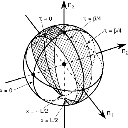
Figure 1: Geometric representation of the periodic instanton.

In the electroweak theory conformal invariance is broken in the Higgs sector which then makes possible the existence of a classical sphaleron solution. In the $O(3)$ sigma model the conformal invariance can be broken by adding to the action (4) the term

$$S_{1}={m^{2}\over g^{2}}\int d^{2}x(1+n_{3})\;,$$ (5)

which also violates the O(3) symmetry and fixes the vacuum state to be $n^{a\,(vac)}=(0,0,-1)$. With the conformal symmetry breaking term (5), the modified model with total action $S=S_{0}+S_{1}$ possesses the classical sphaleron solution [5]

$$n^{(sph)}_{a}(x)=\biggl{(}-2{\mbox{sh}(mx)\over\mbox{ch}^{2}(mx)},\,0\,,-1+{2\over\mbox{ch}^{2}(mx)}\biggr{)}\;,$$ (6)

which has the energy

$$E_{sph}={8m\over g^{2}}\,.$$ (7)

Geometrically, this solution maps the infinite spatial line onto a great circle beginning and ending at the south pole in Fig. 1.

The spectrum of perturbations around the sphaleron has exactly one normalizable negative mode with the eigenfunction $u_{a}(x)=(0,\,\mbox{ch}^{-2}(mx),\,0)$ and the eigenvalue $\omega_{-}^{2}=-3m^{2}$. Because of the existence of this negative mode it is possible to determine the form of the periodic instanton for energies just below the sphaleron energy (7). Adding a small amplitude $\epsilon$ of the negative mode to the static sphaleron gives a Euclidean time-dependent periodic instanton solution,

$$n^{(sph)}_{a}(x)+\epsilon\;{\sin}(|\omega_{-}|\tau)u_{a}(x)$$ (8)

with an energy just below the sphaleron energy. The period of the periodic instanton approaches the critical value $\beta_{crit}=2\pi/|\omega_{-}|=2\pi/(\sqrt{3}m)\approx 3.628/m$ as $\epsilon\rightarrow 0$ and the energy approaches the sphaleron energy, $E\rightarrow E_{sph}$.

In the other limit of very low energies, $E\ll E_{sph}$, the periodic instanton solution can be found by considering an infinite chain of instanton-anti-instanton pairs on the Euclidean time axis. The infinite chain acts as a set of images for the field configuration in one link with fundamental period $\beta$. The classical action of this approximate solution over the fundamental period is

$$S(\beta)\approx{8\pi\over g^{2}}\Bigl{(}1-\pi^{2}{\rho^{2}\over\beta^{2}}-m^{2}\rho^{2}\ln(m\rho)\Bigr{)}\ .$$ (9)

The corrections to the action are suppressed by factors of $m^{2}\beta^{2}$, $m^{2}\rho^{2}$ and $\rho^{2}/\beta^{2}$ which all go to zero for $E\ll E_{sph}$, as we shall see in a moment. Substituting this action into the expression for the rate of tunneling transitions at fixed energy, (2) gives

$$P(E)\sim\exp\Bigl{(}-{1\over g^{2}}W\Bigr{)}$$ (10)

with

$$W=8\pi-g^{2}\beta E-8\pi^{3}{\rho^{2}\over\beta^{2}}-8\pi m^{2}\rho^{2}\ln(m\rho)\$$ (11)

where the values of the period $\beta$ and the instanton size $\rho$ are determined by the saddle-point equations [1]

$${\partial{W}\over\partial{\beta}}={\partial W\over\partial{\rho}}=0.$$ (12)

In the limit $E\ll E_{sph}$ we find

$$\beta(E) \approx {1\over m}\biggl{\{}{2\pi^{2}\over\ln(m/g^{2}E)}\biggr{\}}^{1/2},$$ (13)

$$\rho(E) \approx {(g^{2}E/m)^{1/2}\over 2^{5/4}m}\biggl{\{}{1\over\ln(m/g^{2}E)}\biggr{\}}^{3/4},$$ (14)

which implies

$$W(E)\approx 8\pi-{g^{2}E\over m}\biggl{\{}{2\pi^{2}\over\ln(m/g^{2}E)}\biggr{\}}^{1/2}\ ,$$ (15)

and justifies the neglect of the corrections to the action in the limit of very small energies.

This approximate behavior of the periodic instanton at low energy leads us to observe that the conformal symmetry breaking term in the action (5) serves only to fix the scale of energy and instanton size. It does not distort the periodic instanton from the configuration obtained by a simple linear superposition of zero energy instanton-anti-instanton pairs of the model with unbroken symmetry. This is possible only because $\beta(E)$ goes to zero as $E\rightarrow 0$, i.e., $\beta(E)$ is an increasing function of energy,

$${d\beta(E)\over dE}>0\ .$$ (16)

Notice that this behavior is nevertheless consistent with the linear superposition or dilute gas approximation because the parameter that controls the validity of this approximation is $\rho^{2}/\beta^{2}$, and $\rho$ goes to zero even faster than $\beta$ as $E\rightarrow 0$. Hence it is already clear that the behavior of the periodic instantons in the $O(3)$ model is very different from that of systems with only one quantum mechanical degree of freedom or the abelian Higgs model. In those models $\beta(E)\rightarrow\infty$ as $E\rightarrow 0$, and the periodic instanton contributes to the transition rate as the temperature $\beta^{-1}$ goes smoothly to zero [6]. Periodic instantons in the present model with period going to zero as $E\rightarrow 0$ cannot contribute to the low temperature transition rate, although they can contribute, and in fact dominate transitions between non-thermal low energy states. We shall see presently that the behavior of the period with energy (16) persists up to the sphaleron energy.

At energy comparable, but not very close to the sphaleron energy, the periodic instanton solution has to be found numerically. For that one must solve the Euclidean field equations

$$-(\partial_{\tau}^{2}+\partial_{x}^{2})n_{a}+m^{2}\delta_{a3}-\lambda n_{a}=0,$$ (17)

together with the constraint,

$$n_{a}n_{a}=1\,.$$ (18)

Here, $\lambda$ is a Lagrange multiplier enforcing the constraint, which is easily found by multiplying (17) by $n_{a}$ and using (18). The periodic instanton solution we seek has vanishing time derivative at initial time $\tau=0$, evolves to another turning point at half-period $\beta/2$ where it reflects and then returns to its initial configuration at $\tau=\beta$ by simply reversing the sign of all $\tau$ derivatives. Thus we enforce the half-period boundary conditions,

$${\partial n_{a}(\tau=0,x)\over\partial\tau}={\partial n_{a}(\tau=\beta/2,x)\over\partial\tau}=0\ .$$ (19)

This removes the time translation invariance of the solution. The other boundary condition we require is that at spatial infinity the solution approaches the vacuum. Since we shall work in a finite box of length $L$ we require,

$$n_{a}(\tau,x=-L/2)=n_{a}(\tau,x=L/2)=n^{(vac)}_{a}=(0,0,-1)$$ (20)

for $mL\gg 1$.

Figure 2: The finite rectangular region $(\tau,x)$ of coordinate space that maps onto the shaded region of the sphere in Fig. 1.

Geometrically, the periodic instanton solution obeying these boundary conditions maps the rectangular region of $(\tau,x)$ coordinate space pictured in Fig. 2 into the shaded region of the sphere in Fig. 1. From these figures it should be clear that the solution may be chosen to have well-defined symmetry properties under reflection through the lines bisecting the rectangular region of Fig. 2, so that at $x=0$, $n_{1}$ vanishes while $n_{2}$ and $n_{3}$ reach extrema, and at $\tau=\beta/4$, $n_{2}$ vanishes while $n_{1}$ and $n_{3}$ reach extrema. Imposing these symmetries fixes completely the spatial translational invariance and rotation invariance around the $n_{3}$ axis of the solution, as well as reduces the region we must consider to only one quarter of the full rectangle in Fig. 2. Hence we must solve the differential eqs. (17) subject to the boundary conditions,

$$\begin{array}[]{lcl}x=-L/2&:&n_{1}=0;\;\;n_{2}=0;\;\;n_{3}=-1;\\ t=0&:&dn_{1}/dt=dn_{2}/dt=dn_{3}/dt=0;\\ x=0&:&n_{1}=0;\;\;dn_{2}/dx=dn_{3}/dx=0;\\ t=\beta/4&:&n_{2}=0;\;\;dn_{1}/dt=dn_{3}/dt=0.\end{array}$$ (21)

The lattice version of eqs. (17) can be obtained by a variational principle starting from the discretized action. Let $(t_{i},x_{j})$, where $i=0,\ldots,I$ and $j=0,\ldots,J$ , be the coordinates of lattice sites. The lattice version of the action (4-5) reads

$$S=\sum\limits_{i,j}\Bigl{\{}{1\over 2}(n^{a}_{i+1,j}-n^{a}_{ij})^{2}{d\tilde{x}_{j}\over dt_{i}}+{1\over 2}(n^{a}_{i,j+1}-n^{a}_{ij})^{2}{d\tilde{t}_{i}\over dx_{j}}+m^{2}(1+n^{3}_{ij})d\tilde{t}_{i}d\tilde{x}_{j}\Bigr{\}}$$ (22)

where we have used the notations $dt_{i}=t_{i+1}-t_{i}$, $d\tilde{t}_{i}=(1/2)(dt_{i-1}+dt_{i})$ and similarly for $dx_{j}$, $d\tilde{x}_{j}$.

The equations which follow from the action (22) can be written in the form

$$[B^{a}(\delta^{ab}-n^{a}n^{b})]_{ij}=0,$$ (23)

where

$$B^{a}_{ij}\equiv-{n^{a}_{i+1,j}\over d\tilde{t}_{i}dt_{i}}-{n^{a}_{i-1,j}\over d\tilde{t}_{i}dt_{i-1}}-{n^{a}_{i,j+1}\over d\tilde{x}_{j}dx_{j}}-{n^{a}_{i,j-1}\over d\tilde{x}_{j}dx_{j-1}}+m^{2}\delta_{a3}.$$ (24)

Eqs. (23) actually contain only two independent equations since its projection onto the vector $n^{a}_{ij}$ is identically zero. Together with the constraint equation (18) these comprise a complete set of three independent equations associated with each lattice site. From eqs. (23) it is clear that $B^{a}$ must be parallel to $n^{a}$ at each point $(i,j)$. Since $n^{a}$ is normalized to unity, the eqs. (23)–(24) can be rewritten in the equivalent, symmetric form,

$$n^{a}\sqrt{B^{c}B^{c}}+B^{a}=0,$$ (25)

for every $(i,j)$. This form is more convenient for numerical calculations.

To obtain a numerical solution of (25) we use Newton’s method. That is, we

1. choose an initial field configuration as a first guess;

2. linearize the equations in the background of the initial field;

3. solve the linearized equations to obtain an improved configuration; and

4. iterate until the procedure converges.

The choice of initial configuration is guided by the known behavior of the periodic instanton solution near $E=0$ and $E=E_{sph}$. For example, for $E$ just below $E_{sph}$ an initial configuration of the form (8) with $\epsilon\sim 0.5$ works well. The convergence of the scheme is quadratic, and double precision accuracy is typically reached in $5$ to $7$ iterations.

The solution of the linearized equations in step (3) of the algorithm requires an inversion of the matrix of small fluctuations about the trial configuration. Negative eigenvalues of this matrix are treated on the same footing as positive eigenvalues, and pose no special problem for Newton’s method, which is important for the present application. Because of the boundary conditions which fix the translational and rotational symmetries there are no zero eigenvalues of the matrix near the desired solution, which otherwise would be disastrous for this method.

For a $I\times J$ spacetime grid the matrix to be inverted has $I^{2}J^{2}$ elements. In general, it takes of order $I^{3}J^{3}$ operations to invert such a matrix. However, the sparseness of the matrix makes it more efficient to follow a procedure of forward elimination and back substitution along either the $x$ or $\tau$ directions instead. That is, starting with one edge of the region in Fig. 2, such as $\tau=0$, we solve for each $\tau$ slice of the grid in terms of the successive two $\tau$ slices until the edge $\tau=\beta/4$ is reached, where the boundary condition determines the unknown quantities. Then we reverse direction and solve for the unknowns on the previous $\tau$ slices successively. This allows for the matrix to be inverted in order $IJ^{3}$ operations (or $I^{3}J$ operations if the $x$ direction is chosen), and speeds up the algorithm considerably. In practice, a grid size of order $100\times 100$ can be handled on a typical workstation, which already provides reasonable accuracy ($\sim 1\%$) for the problem at hand.

The numerical method described works quite well and yields a periodic instanton solution for energies in the range of $1$ to $8$ in units of $m/g^{2}$. Smaller energies require finer lattices to obtain the same accuracy, since the instanton size becomes smaller. The results of our calculations are summarized in Figs. 3. They were obtained on a $40\times 40$ grid in a spatial box of size $L=8$ in units of $m^{-1}$.

Fig. 2 illustrates a typical periodic instanton solution. As one can see, at the turning points $\tau=0$ and $\tau=\beta/2$ the field configuration is non-vacuum, and the components of the vector $n^{a}$ cover the shaded patch of the sphere in Fig. 1.

Fig. 3a shows the dependence of the action of the periodic instanton, in units of $1/g^{2}$, on its half-period, as the latter varies from $\beta/2\sim 1.3$ to $\beta/2\sim\beta_{crit}/2$. The action grows smoothly from a value close to $S_{0}=4\pi$ to $\beta_{crit}E_{sph}/2\approx 14.5$.

Fig. 3b shows the dependence of the half-period $\beta/2$ as a function of energy. Near the sphaleron energy ($8$ in units $m/g^{2}$), the period reaches the critical period $\beta_{crit}$.

Fig. 3c shows the exponent, $W=S-E\beta$, in the suppression factor for the tunneling probability $P(E)$, as a function of energy. $W$ varies from a value slightly below $4\pi$ at low energies to zero at $E\sim E_{sph}$.

Figure 3: (a) Action of periodic instanton versus half-period.

Figure 3: (b) Half-period versus energy for the periodic instanton.

Figure 3: (c) The suppression factor $W$ (in $P(E)$) as a function of energy.

The behavior of all quantities in these graphs is smooth, so that greater accuracy may be obtained in a straightforward way by increasing the number of lattice sites.

The periodic instanton solutions we have found numerically dominate the winding number transition rate at fixed energy. At fixed temperature, the transition rate is given to exponential accuracy by

$$\Gamma(T)=\int_{0}^{\infty}dE\,e^{-E/T}P(E),$$ (26)

where $T$ is the temperature. Evaluating this integral by the method of steepest descent (which is valid in the limit of arbitrarily weak coupling $g^{2}\rightarrow 0$ provided $T$ is coupling independent) gives the saddle point condition

$$T^{-1}=-{dW\over dE}=\beta(E)\ .$$ (27)

However, evaluating the second derivative of the exponent at this saddle point yields

$$-{d^{2}W\over dE^{2}}=+{d\beta(E)\over dE}>0\ ,$$ (28)

which tells us that this extremum is a minimum of the exponent rather than a maximum, for the periodic instanton solutions we have found obeying (16). Hence this saddle point does not give the dominant contribution to the rate $\Gamma$, and the periodic solutions we have found are not the relevant ones for finite temperature transitions.

If these periodic solutions are the only ones obeying the saddle point periodicity condition (27), then the integral in eq. (26) is saturated either at $E=0$, which implies

$$\Gamma(T)\sim\exp(-2S_{0})=\exp(-8\pi)\;,$$

or at $E=E_{sph}$, where the exponent $W(E)$ reaches zero and the exponential suppression in $P(E)$ disappears. In the latter case one finds

$$\Gamma(T)\sim\exp(-E_{sph}/T)\;.$$

The crossover between these two cases occurs when the two contributions become equal, i.e., at

$$T_{cr}={E_{sph}\over 2S_{0}}={m\over\pi}\;.$$

At temperatures above $T_{cr}$ the transition rate is dominated by the thermal activation over the top of the barrier, and the sphaleron solution plays a dominant role. At temperatures less than $T_{cr}$, the transition rate coincides with the zero energy tunneling rate. At temperatures $T<T_{cr}$ there would then be no exact classical solution which dominates the finite temperature transition rate, and we would expect instead that the field configurations which saturate the rate at $T<T_{cr}$ are the same as those saturating the zero temperature transition rate, viz., the constrained instantons [7] which are not exact solutions to the Euclidean field equations. Indeed, at $T=0$ the absence of any exact real finite action solutions immediately follows from scaling arguments (Derrick’s theorem), and at finite $T$ imposing periodic boundary conditions at Euclidean time $T^{-1}$ does not alter this argument as long as $T\ll m$.

The other possibility is that the real periodic instanton solutions we have considered in this letter are not the only solutions to the field equations satisfying the periodicity condition (27), but that there are other solutions, perhaps complex, for which the periodicity decreases with increasing energy, and which do dominate the finite temperature rate $\Gamma(T)$. Since we know that at sufficiently low temperatures there are no other real periodic solutions than the ones we have found, any other solutions would have to be complex, in order to evade the scaling argument. Indeed it is interesting to speculate that the reason the constrained instanton configurations can dominate the zero temperature transition rate even though they are not exact solutions is that they are a good approximation (in their action) to some exact complex solution to the field equations, yet to be discovered. If this speculation is correct, then we would have to reconsider the question of whether the real periodic solutions obeying the boundary conditions (21) are the correct configurations maximizing the transition probability at fixed energy as well.

We would like to conclude by stressing the analogy between the two dimensional sigma model with the symmetry breaking term (5) and the spontaneously broken $SU(2)$ gauge theory. In both cases, in the unbroken phase, instanton solutions exist and can have arbitrary size. In the broken phase, exact real instanton solutions do not exist, and the dominant contribution to the zero temperature (energy) transition rate comes from approximate solutions, the constrained instantons. Like in the sigma model, in the spontaneously broken $SU(2)$ gauge theory the period of the periodic instanton increases with energy at low energies, where perturbation theory is applicable [1]. Hence the situation is in all important respects exactly the same as in our broken $O(3)$ sigma model, and one may expect that the finite temperature transition rate in the $SU(2)$ + Higgs system is saturated either by zero energy tunneling or by sphaleron activation, with a sharp crossover between these two regimes at temperatures of order $M_{W}$, or else new complex periodic solutions to the equations of motion of the $SU(2)$- Higgs system exist which are still awaiting discovery.

The authors are grateful to M. Shaposhnikov and V. Rubakov for enlightening discussions. One of us (P.T.) wishes to thank D. T. Son, A. Kuznetsov, and S. Khlebnikov for helpful discussions, and the Theory Division of CERN for hospitality. The work of P.T. is supported in part by the Russian Foundation for Fundamental Research (project 93-02-3812) and by the International Science Foundation. E.M. and S.H. acknowledge support from the United States Department of Energy. This research was performed in part using the resources located at the Advanced Computing Laboratory, Los Alamos National Laboratory.

References

- [1] S. Yu. Khlebnikov, V. A. Rubakov and P. G. Tinyakov, Nucl. Phys. B 367, 334 (1991).
-
[2]
V. A. Rubakov and P. G. Tinyakov, Phys. Lett. 279B, 165 (1992);
P. G. Tinyakov, Phys. Lett. 284B, 410 (1992);
V. A. Rubakov, D. T. Son, and P. G. Tinyakov, Phys. Lett. 287B, 342 (1992). - [3] V. V. Matveev, Phys. Lett. 304B, 291 (1993).
- [4] A. A. Belavin and A. M. Polyakov, Pisma ZhETF 22, 245 (1975).
- [5] E. Mottola and A. Wipf, Phys. Rev. D 39, 588 (1989).
- [6] I. Affleck, Phys. Rev. Lett. 46, 388 (1981).
- [7] I. Affleck, Nucl. Phys. B 191, 429 (1981).