CERN-TH.7306/94
SISSA 83/94/EP

Studying $\varepsilon^{\prime}/\varepsilon$ in the Chiral Quark Model:
$\gamma_{5}$-Scheme Independence and NLO Hadronic Matrix Elements

Stefano Bertolini

INFN, Sezione di Trieste, and
Scuola Internazionale Superiore di Studi Avanzati
Via Beirut 4, I-34013 Trieste, Italy

Jan O. Eeg and Marco Fabbrichesi

CERN, Theory Division
CH-1211 Geneva 23, Switzerland

Abstract

We study the $CP$-violating, $|\Delta S|=1$ parameter $\varepsilon^{\prime}/\varepsilon$ by computing the hadronic matrix elements in the chiral quark model. We estimate in the chiral expansion the coefficients of the next-to-leading order terms that correspond to the operators $Q_{6}$ and $Q_{11}$. We consider the impact of these corrections on the value of $\varepsilon^{\prime}/\varepsilon$. We also investigate the possibility that the chiral quark model might drastically reduce the dimensional regularization $\gamma_{5}$-scheme dependence of current evaluations of $\varepsilon^{\prime}/\varepsilon$.

CERN-TH.7306/94
SISSA 83/94/EP
August 1994

1 Foreword and Summary

A detailed study of the $CP$-violating, $|\Delta S|=1$ parameter $\varepsilon^{\prime}/\varepsilon$ puts us at the crossroad of different aspects of standard model physics and, accordingly, provides a promising testing ground of model-dependent features.

As the precision in the experimental measurements of $\varepsilon^{\prime}/\varepsilon$ improves [1], all theoretical predictions face the challenge of reducing their uncertainties. These have a twofold origin as, on the one hand, the analysis of the Wilson coefficients must be pushed to higher orders in $\alpha_{s}$ and $\alpha$ (as well as including all the relevant operators) while, on the other hand, the estimate of the hadronic matrix elements has to be substantially improved.

Indeed, a great deal of work has been done in this direction. In recent years the Wilson coefficients of the effective lagrangian for $|\Delta S|=1$ weak decays have been computed to the next-to-leading order (NLO) [2, 3], and matrix elements have been calculated by a variety of techniques like $1/N_{c}$ [4], quark models [5] and lattice [3]. Yet it is perhaps fair to say that, all efforts notwithstanding, the current uncertainty in the theoretical prediction of $\varepsilon^{\prime}/\varepsilon$ is still large, most of it arising from the hadronic matrix elements.

There are at least four relevant perturbative expansions which are important in estimating hadronic matrix elements. These are the $1/N_{c}$ and $\alpha_{s}/\pi$ expansions for non-factorizable contributions, which have been studied in [4] and [5], respectively. Then we have the chiral expansion, which comes in two varieties according to the energy scale at which it is considered. The coefficients of the chiral lagrangian take contributions from chiral loops (corresponding to momenta below the scale $\Lambda_{QCD}$ at which all quark fields are integrated out) as well as from light-quark loops (between $\Lambda_{QCD}$ and the chiral symmetry breaking scale $\Lambda_{\chi}$).

The chiral quark model ($\chi$QM) [6, 7, 8] can be thought as interpolating between the lower-end of the perturbative short-distance analysis ($\approx 1$ GeV) and the chiral lagrangian energy region ($\Lambda_{QCD}\approx M$). In the model, the scale $M$ is identified with the constituent quark mass. This is the only free parameter in our analysis and most matrix elements are a sensitive function of it. What are the allowed values for this parameter? As we shall discuss in section 2, a rather large range ($100<M<400$ MeV) is possible, different analyses having different outcomes according to the actual physical processes considered.

In this paper, we begin a study of $\varepsilon^{\prime}/\varepsilon$ in the $\chi$QM by focusing on two aspects: the relevance of the NLO corrections to the hadronic matrix elements and the problem of the $\gamma_{5}$-scheme independence of the estimate. Our original motivation was to study the gluonic magnetic dipole penguin operator

$$Q_{11}\simeq\frac{g_{s}}{16\pi^{2}}\,m_{s}\>\overline{s}\,\sigma_{\mu\nu}t^{a}G^{\mu\nu}_{a}(1-\gamma_{5})\,d\,,$$ (1.1)

which until recently has been tacitly neglected in all discussions of $\varepsilon^{\prime}/\varepsilon$. The potential relevance of the operator $Q_{11}$ for $\varepsilon^{\prime}/\varepsilon$ has been discussed in a previous work [9]. We confirm the result of ref. [9] up to an overall sign. In section 3 we discuss in detail the bosonization of $Q_{11}$. The first non-vanishing contribution of $Q_{11}$ to the $K\to\pi\pi$ matrix elements comes from a term that is NLO in the chiral expansion (O$(p^{4})$). Even though the corresponding coefficient of the chiral expansion—as well as the short-distance Wilson coefficient—is large, the matrix element turns out to be kinematically suppressed by a factor $m_{\pi}^{2}/m_{K}^{2}$ with respect to the dominant operators, making its contribution to $\varepsilon^{\prime}/\varepsilon$ subleading.

In order to better gauge the significance of this NLO contribution, we estimate, in section 4, the NLO correction to the matrix element of the ordinary gluonic penguin operator

$$Q_{6}=\overline{s}_{\alpha}\gamma_{\mu}(1-\gamma_{5})d_{\beta}\sum_{q}\overline{q}_{\beta}\gamma^{\mu}(1+\gamma_{5})q_{\alpha}\,,$$ (1.2)

which gives the dominant contribution to $\varepsilon^{\prime}/\varepsilon$. Such an NLO correction to the hadronic matrix element of $Q_{6}$ turns out to be generally larger than the contribution of the operator $Q_{11}$, as well as the leading-order (LO) contributions of the operators $Q_{3}$, $Q_{5}$ and $Q_{7}$ (see section 5 for definitions). Its size increases monotonically with $M$, ranging from 14% of the LO term for $M=120$ MeV up to 25% and more for $M\ \raisebox{-1.72218pt}{\hbox to0.0pt{$\sim$\hss}}\raisebox{1.72218pt}{$>$}\ 220$ MeV. Our perturbative results (we perform an expansion in powers of $M^{2}/\Lambda_{\chi}^{2}$) should not be trusted for larger values of $M$, higher-order corrections being needed.

Our approach makes it also possible to study the dimensional regularization $\gamma_{5}$-scheme dependence of the matrix elements of these operators. This is an important problem since it causes, if we take the NLO results for the Wilson coefficients in the two schemes, a significant part of the current theoretical uncertainty (see for instance ref. [2])—as large as 70–80% for $m_{t}=170$ GeV. One expects this scheme dependence to disappear when matrix elements are consistently evaluated [10]. This cannot be done within the lattice or $1/N_{c}$ approach.

As a preliminary analysis, in section 5 we use the $\chi$QM to study the $\gamma_{5}$-scheme dependence of $\varepsilon^{\prime}/\varepsilon$ in a toy model, made of the LO matrix elements of the operators $Q_{6}$ (for the $I=0$ amplitude) and of the electroweak penguin operator (for $I=2$):

$$Q_{8}=\frac{3}{2}\,\overline{s}_{\alpha}\gamma_{\mu}(1-\gamma_{5})d_{\beta}\sum_{q}e_{q}\ \overline{q}_{\beta}\gamma^{\mu}(1+\gamma_{5})q_{\alpha}\,,$$ (1.3)

which becomes important for a heavy top quark. As a matter of fact, the Wilson coefficients of these two operators exhibit the largest scheme dependence. In comparison, the scheme dependence of the Wilson coefficients of $Q_{4}$ and $Q_{9}$, next in relevance to $Q_{6}$ and $Q_{8}$, is ten times smaller.

We find that the $\gamma_{5}$-scheme dependence of $\varepsilon^{\prime}/\varepsilon$ in our toy model is reduced below the 10% level for values of the parameter $M$ well within the allowed range. This means that, for any value of $\Lambda_{QCD}^{(4)}$ in the 200–400 MeV range and of the renormalization scale $\mu$ between 1 GeV and $m_{c}$, it is possible to find a value of $M$ in a restricted range (120–220 MeV) for which the scheme dependence of the hadronic matrix elements exactly cancels that of the Wilson coefficients.

Notice that in the $\chi$QM the matrix element of $Q_{11}$ turns out to be scheme-independent, as it happens for its “LO” Wilson coefficient [11].

The range of values for which we find scheme independence is consistent with the values of $M$ for which we can trust our perturbative results at the order $M^{2}/\Lambda_{\chi}^{2}$ ($M\ \raisebox{-1.72218pt}{\hbox to0.0pt{$\sim$\hss}}\raisebox{1.72218pt}{$<$}\ 200$ MeV). To extend our analysis in a reliable manner to values of $M$ of 300 MeV and more requires considering higher-loop effects—a difficult computational problem.

As encouraging as these results might be, we should remember that we are considering a toy model for $\varepsilon^{\prime}/\varepsilon$ in which only the two leading operators $Q_{6}$ and $Q_{8}$ are included. In order to ascertain conclusively the scheme independence and the size of $\varepsilon^{\prime}/\varepsilon$, all relevant operators should be evaluated in the $\chi$QM and consistently included. Preliminary estimates show that such an extension stabilizes the range of values of $M$ for which the scheme independence is substantially weakened, further reducing the renormalization scale dependence.

In the final part of the paper (section 6) we compare the contribution to $\varepsilon^{\prime}/\varepsilon$ of the dipole penguin operator $Q_{11}$ to the other ten traditional operators. Since the hadronic matrix elements of the other operators beside $Q_{6}$ are known in the $\chi$QM only to the leading factorizable order, we follow for the ten traditional operators the $1/N_{c}$ approach of ref. [2].

A detailed anatomy of all individual contributions is summarized in tables 6, 7 and 8. We find these tables a useful way of displaying the available information and a standard reference for future developments.

The Wilson coefficients are computed to the NLO level, at least to the extent made possible by the entries of the anomalous dimensions currently available—the three-loop NLO mixing between $Q_{11}$ and the other operators and related two-loop initial conditions are still missing. This may amount to a 40–50% uncertainty in the $Q_{11}$ Wilson coefficient at the 1 GeV scale (extrapolating the results for $b\to s\gamma$ given in ref. [12]). Nonetheless, this little affects the final result for $\varepsilon^{\prime}/\varepsilon$ since the evolution of the first ten Wilson coefficients is independent on the presence of the $Q_{11}$ (and $Q_{12}$) operator.

Our analysis shows that the inclusion of the magnetic penguin operator affects the prediction of $\varepsilon^{\prime}/\varepsilon$ always below the $10^{-4}$ level, therefore putting $Q_{11}$ in the same class as other operators like $Q_{3}$, $Q_{5}$ and $Q_{7}$, whose contributions are even smaller; yet, for $m_{t}\ \raisebox{-1.72218pt}{\hbox to0.0pt{$\sim$\hss}}\raisebox{1.72218pt}{$>$}\$ 170 GeV, the size of $\varepsilon^{\prime}/\varepsilon$ itself becomes of the same order as the $Q_{11}$ contribution.

The completion of the study of $\varepsilon^{\prime}/\varepsilon$ in the $\chi$QM approach is needed to ascertain conclusively the $\gamma_{5}$-scheme independence of the result and, what is equally relevant, the corresponding size of $\varepsilon^{\prime}/\varepsilon$. Corrections of the order of the current quark masses and $\alpha/\pi$ will then have to be included. We expect the mass corrections to be of the order or less than 10%, while those of (soft) gluon contributions to be larger ($\ \raisebox{-1.72218pt}{\hbox to0.0pt{$\sim$\hss}}\raisebox{1.72218pt}{$<$}\ 50$%). We recall that in our toy model we find systematically a factor of 3–4 enhancement with respect to the average of the $1/N_{c}$ results with $Q_{6}$ and $Q_{8}$ only and $m_{t}=170$ GeV. This is partially due to a reduced cancellation between the two operators in the $\chi$QM.

We also stress the relevance of the calculation of NLO corrections to all relevant matrix elements, which become crucial for $m_{t}\ \raisebox{-1.72218pt}{\hbox to0.0pt{$\sim$\hss}}\raisebox{1.72218pt}{$>$}\ 170$ GeV, due to the large cancellations that occur between gluonic and electromagnetic penguin contributions.

2 Bosonization of quark operators

In general, the effective lagrangian at the quark level has the form

$${\cal{L}}_{Q}\,=\,\sum_{i}\,C_{i}\;Q_{i}\;,$$ (2.1)

where the coefficients $C_{i}$ contain the short-distance physics above the renormalization point $\mu\simeq 1$ GeV, and $Q_{i}$ are operators containing quark fields (at the scale $\mu$). When the quark operators are bosonized, they will be represented by some linear combination of meson operators ${\cal{L}}_{j}^{(\chi)}$:

$$Q_{i}\,\rightarrow\,\sum_{j}\,b_{ij}\;{\cal{L}}_{j}^{(\chi)}\,,$$ (2.2)

leading to the following chiral lagrangian at the meson level:

$${\cal{L}}_{Q}\,\rightarrow\,{\cal{L}}_{\chi\mbox{\scriptsize PT}}\,=\,\sum_{i,j}\,G_{j}(Q_{i})\,{\cal{L}}_{j}^{(\chi)}\,=\,\sum_{j}\,G_{j}\,{\cal{L}}_{j}^{(\chi)}\,,$$ (2.3)

where $G_{j}(Q_{i})\equiv C_{i}\,b_{ij}$ (no sum on $i$).

One way to perform the bosonization is to give the complete list of operators ${\cal{L}}_{j}^{(\chi)}$ to which some quark operator $Q_{i}$ could a-priori contribute [13, 14, 15]. To determine the various coefficients $b_{ij}$, one tries combinations of experimental data and phenomenological estimates. In this work, we have chosen a version of the $\chi$QM advocated by various authors [6, 7]. This type of effective low-energy model is obtained by adding a new term to the ordinary QCD lagrangian:

$${\cal{L}}_{\chi\mbox{\scriptsize QM}}=-M\left(\overline{q}_{R}\;\Sigma q_{L}+\overline{q}_{L}\;\Sigma^{\dagger}q_{R}\right)\;,$$ (2.4)

where $\overline{q}=(\overline{u},\overline{d},\overline{s})$, and the $3\times 3$ matrix $\Sigma\equiv\exp\left(2i\,\Pi/f\right)$ contains the pseudoscalar octet mesons $\Pi=\sum_{a}\pi^{a}\lambda^{a}/2$ $(a=1,..,8)$. The scale $f$ is identified with the (bare) pion decay constant, so that numerically $f\simeq f_{\pi}\simeq 93.3$ MeV (and equal to $f_{K}$ in the chiral limit).

The parameter $M$ is characteristic of the $\chi$QM and represents a typical constituent quark mass for the light quarks. For $M\neq 0$ the chiral symmetry is broken and the quark condensate acquires a non-vanishing vacuum expectation value. A central value of 320 MeV is found in ref. [5], albeit with a comparable uncertainty. Smaller values are found by fitting data relevant to meson physics, as in ref. [16], where $M=223\pm 9$ MeV is quoted. It seems fair to consider the range $100\,\mbox{MeV}<M<400\,\mbox{MeV}$, as a reasonable present-day uncertainty on the determination of the parameter $M$.

The resulting field theory with pseudoscalar quark-meson couplings (see appendix A) and quark loops gives a good description of the $K\rightarrow\pi\pi$ amplitudes to leading order in $1/N_{c}$ [5], and under certain conditions of the anomalous $\pi^{0}\rightarrow\gamma\gamma$ amplitude [17, 16], as well as $K^{0}\rightarrow\gamma\gamma$ [18, 19]. It is also worth recalling that the $\Delta=1/2$ rule in $CP$-conserving kaon decays is reproduced within the model up to factors 2–3 [5], whereas other approaches fail by an order of magnitude.

When performing loop integrals within this model, the logarithmic and quadratic divergences are identified with $f_{\pi}$ and the quark condensate $\langle\overline{q}q\rangle$, respectively, that is:

$$f_{\pi}^{(0)}\,=\,\frac{N_{c}M^{2}}{4\pi^{2}f}\hat{f}_{\pi}\qquad\mbox{and}\qquad\langle\overline{q}q\rangle^{(0)}\,=\,\frac{N_{c}M}{4\pi^{2}}\hat{C}_{q}\;,$$ (2.5)

where $f^{(0)}_{\pi}$ and $\langle\overline{q}q\rangle^{(0)}$ are the pion decay constant and the quark condensate to zeroth order in $\alpha_{s}$ (no gluon-condensate corrections and zero current-quark masses, see eq. (4.20)). We distinguish between $f^{(0)}_{\pi}$ and $f$ because of their different origin, even though at out level of approximation $f^{(0)}_{\pi}=f\simeq f_{\pi}$.

In dimensional regularization ($d=4-2\epsilon$) we have

$$\hat{f}_{\pi}=\frac{1}{\epsilon}-\gamma_{E}+\ln 4\pi+\ln\frac{\mu^{2}}{M^{2}}\qquad\mbox{and}\qquad\hat{C}_{q}=M^{2}(\hat{f}_{\pi}+1)\,.$$ (2.6)

It is perhaps useful to recall that, introducing in the effective theory a cut-off $\Lambda$ one obtains [8]

$$\hat{f}_{\pi}=\log(\Lambda^{2}/M^{2})+...\qquad\mbox{and}\qquad\hat{C}_{q}=-\Lambda^{2}+M^{2}\log(\Lambda^{2}/M^{2})+...$$ (2.7)

To the order we work we cannot remove the cut-off. Equations (2.5) are thus a convenient book-keeping device to identify $f_{\pi}$ and $\langle\overline{q}q\rangle$ in the loop integrals.

The model has a “rotated” picture, where the term ${\cal{L}}_{\chi\mbox{\scriptsize QM}}$ in (2.4) is transformed into a pure mass term $-M\overline{{\cal{Q}}}{\cal{Q}}$ for rotated ”constituent quark” fields ${\cal{Q}}_{L,R}$ :

$$q_{L}\rightarrow{\cal{Q}}_{L}=\xi q_{L}\quad\mbox{and}\quad q_{R}\rightarrow{\cal{Q}}_{R}=\xi^{\dagger}q_{R}\,,$$ (2.8)

where $\xi\,\cdot\,\xi=\Sigma$. The meson–quark couplings in this rotated picture arise from the kinetic (Dirac) part of the constituent quark lagrangian. These interactions can be described in terms of vector and axial vector fields coupled to constituent quark fields ${\cal{Q}}={\cal{Q}}_{R}+{\cal{Q}}_{L}$:

$${\cal{L}}_{int}\,=\,\overline{{\cal{Q}}}\Bigl{[}\gamma^{\mu}{\cal{V}}_{\mu}\,+\,\gamma^{\mu}\gamma_{5}{\cal{A}}_{\mu}\,\Bigr{]}{\cal{Q}}\,,$$ (2.9)

where

$${\cal{V}}_{\mu}\,=\,(R_{\mu}+L_{\mu})/2\,,\qquad{\cal{A}}_{\mu}\,=\,(R_{\mu}-L_{\mu})/2\,,$$ (2.10)

and

$$L_{\mu}\,=\,\xi\,(i\partial_{\mu}\,\xi^{\dagger})+\xi\,l_{\mu}\,\xi^{\dagger}\,,\qquad R_{\mu}\,=\,\xi^{\dagger}(i\partial_{\mu}\xi)+\xi^{\dagger}r_{\mu}\,\xi\,.$$ (2.11)

Here $l_{\mu}$ and $r_{\mu}$ are the external fields containing the photon (as well as the $W$ field).

Using (2.9), the strong chiral lagrangian $O(p^{2})$ can be understood as two axial currents ${\cal{A}}_{\mu}$ attached to a quark loop, leading to

$${\cal{L}}^{(2)}_{s}\,\sim\,\mathop{\mbox{Tr}}\,\Bigl{[}{\cal{A}}_{\mu}\,{\cal{A}}^{\mu}\Bigr{]}\,.$$ (2.12)

Using the relations [16, 20]

$$2i\,{\cal{A}}_{\mu}\,=\;-\,\xi^{\dagger}(D^{\mu}\Sigma)\xi^{\dagger}\;=\;\xi(D_{\mu}\Sigma^{\dagger})\xi\,,$$ (2.13)

one obtains the leading strong chiral lagrangian

$${\cal{L}}^{(2)}_{s}\,=\,\frac{f^{2}}{4}\,\mathop{\mbox{Tr}}\,\Bigl{(}D^{\mu}\Sigma^{\dagger}\,D_{\mu}\Sigma\Bigr{)}\;,$$ (2.14)

where $D_{\mu}$ is the covariant derivative. Note that ${\cal{A}}_{\mu}$ is invariant under local chiral transformations [6], in agreement with the invariance of ${\cal{L}}^{(2)}_{s}$. In contrast, the vector field ${\cal{V}}_{\mu}$ transforms as a gauge field. Therefore, terms involving the vector field would manifestly break local chiral invariance and cannot appear in a chiral lagrangian, except for the anomaly term [19]. The vector field can only be present indirectly through some field tensor obtained from the commutator of the total covariant derivative of the lagrangian. In addition, the covariant derivative of ${\cal{A}}_{\mu}$ may occur in higher-order terms [5, 15, 20, 21].

In the version of the $\chi$QM given by (2.4) (the unrotated picture) the momenta which correspond to derivatives of the fields have to be extracted from the quark propagators in the loop diagram, and it is in general difficult to see the correspondence between the quark and the bosonized version of the operators. The rotated picture, where the axial vector fields in eq. (2.9) couple to the quark loops with derivative couplings, is more transparent in this sense. For example, for $O(p^{4})$ terms (with two momenta and one current quark mass), no momenta have to be extracted from the quark propagators, and we can readily deduce the chiral lagrangian (bosonized quark operator) in terms of the rotated fields.

3 Bosonization of $Q_{11}$

The magnetic dipole operator (1.1) can be rewritten as

$$Q_{11}\,=\,\frac{g_{s}}{8\pi^{2}}\overline{s}\;\Bigl{[}m_{d}\,R+m_{s}\,L\Bigr{]}\,\,\sigma\cdot G\;d\,+\,h.c.\;,$$ (3.1)

where $\sigma\cdot\,G\equiv\sigma^{\mu\nu}\,G^{a}_{\mu\nu}t^{a}$, $G^{a}_{\mu\nu}$ is the gluon field, $t^{a}$ are the SU(3) generators, normalized as $\mathop{\mbox{Tr}}\,(t^{a}t^{b})=(1/2)\delta^{ab}$, and $(L,R)=(1\mp\gamma_{5})/2$. The Hermitian conjugate is there to remind us of the corresponding $s\rightarrow d$ transition. This will be understood throughout the paper. The dipole operator in eq. (3.1) can be written in a chiral $SU(3)$ covariant form as

$$Q_{11}\,=\,\frac{g_{s}}{8\pi^{2}}\,\Bigl{[}\overline{q}_{R}\;{\cal{M}}_{q}\lambda_{-}\;\sigma\cdot G\,q_{L}\,+\,\overline{q}_{L}\;\;\sigma\cdot G\;\lambda_{-}{\cal{M}}_{q}^{\dagger}\;q_{R}\Bigr{]}\,,$$ (3.2)

where ${\cal{M}}_{q}\,=\,\mbox{diag}\,(m_{u},m_{d},m_{s})$ is the current quark matrix. The Gell-Mann matrices $\lambda_{\pm}\,=\,(\lambda_{6}\pm i\,\lambda_{7})/2$ project $\Delta S\,=\,\pm 1$ transitions out of the quark fields $\overline{q}_{L}\,=\,(\overline{u}_{L},\,\overline{d}_{L},\,\overline{s}_{L})$. Note that in eq. (3.2) the operator transforms as $(\underline{8}_{L},\underline{1}_{R})$ under the chiral $SU(3)_{L}\times SU(3)_{R}$ symmetry if the current quark matrix is taken to transform as ${\cal{M}}_{q}\to U_{R}{\cal{M}}_{q}U_{L}^{\dagger}$, where $U_{R}$ and $U_{L}$ are the chiral $SU(3)$ transformation matrices.

In the rotated picture, $Q_{11}$ reads

$$Q_{11}\,=\,\frac{g_{s}}{8\pi^{2}}\,\overline{{\cal{Q}}}\Bigl{[}F_{(-)}^{V}\,+\,F_{(-)}^{A}\,\gamma_{5}\Bigr{]}\>\sigma\cdot G\;{\cal{Q}}\,,$$ (3.3)

where $F_{(-)}^{V,A}=\left(F_{(-)}^{R}\pm F_{(-)}^{L}\right)/2$, with

$$F_{(-)}^{L}\;=\,\xi^{\dagger}\,{\cal{M}}_{q}\lambda_{-}\xi^{\dagger}\,,\qquad\mbox{and}\qquad F_{(-)}^{R}\;=\;\xi\,\lambda_{-}{\cal{M}}_{q}^{\dagger}\,\xi\,.$$ (3.4)

The operator corresponding to $Q_{11}$ is understood in terms of a quark loop. Let us first note that the lowest-order contribution is given by a quark loop where only the field $F_{(-)}^{V}$ is interacting

$${\cal{L}}^{(2)}(Q_{11})\,\sim\,\mathop{\mbox{Tr}}\,(F_{(-)}^{V})\;=\;\mathop{\mbox{Tr}}\,\Bigl{[}\Sigma^{\dagger}\,{\cal{M}}_{q}\,\lambda_{-}+\lambda_{-}\,{\cal{M}}_{q}^{\dagger}\,\Sigma\Bigr{]}\;.$$ (3.5)

This is the contribution that cancels against the pole term induced by a non-vanishing $\langle 0|Q_{11}|K^{0}\rangle$ transition [22], in agreement with the FKW theorem [23]. To the NLO, we obtain a term corresponding to an interaction of $F_{(-)}^{V}$ and two axial fields attached to a quark loop:

$${\cal{L}}^{(4)}(Q_{11})\,\sim\,\mathop{\mbox{Tr}}\,\Bigl{[}F_{(-)}^{V}{\cal{A}}_{\mu}\,{\cal{A}}^{\mu}\Bigr{]}\,.$$ (3.6)

Note that $F_{(-)}^{A}$ is not contributing in eqs. (3.5)–(3.6), because there must be an even number of $\gamma_{5}$’s in the quark loop. Using (2.13) and (3.4), we find that ${\cal{L}}^{(4)}(Q_{11})$ can be written in the form

$${\cal{L}}^{(4)}(Q_{11})=G_{\underline{8}}^{(4)}(Q_{11})\,\mathop{\mbox{Tr}}\,\Bigl{[}\left(\Sigma^{\dagger}\,{\cal{M}}_{q}\lambda_{-}+\lambda_{-}{\cal{M}}_{q}^{\dagger}\Sigma\right)\,D^{\mu}\Sigma^{\dagger}D_{\mu}\Sigma\Bigr{]}\,.$$ (3.7)

In eq. (3.2), we see that $\lambda_{-}$ and ${\cal{M}}_{q}$ are always next to each other, and so they must be in the bosonized version of $Q_{11}$. We neglect the possible terms appearing as the product of two traces. The latter correspond to two quark loops connected by (soft) gluons and will therefore be suppressed by a factor $(\alpha_{s}/\pi)^{2}$, at least. Due to the $CPS$ symmetry [24] of the quark operators, also the corresponding bosonized operators have to exhibit such a symmetry. As a consequence the two terms in eq. (3.7) must appear with equal weight. Among all the possible terms for $|\Delta S|=1$ kaon decays, which can be obtained by inserting the flavor-changing matrix $\lambda_{-}$ into various places within the trace in ${\cal{L}}^{(4)}_{s}$ [15], we are thus left with the unique term in eq. (3.7).

The coefficient in eq. (3.7) can be most easily calculated in the unrotated picture, by considering, for instance, the off-shell $K\rightarrow\pi$ transition. In order to calculate $G_{\underline{8}}^{(4)}(Q_{11})$, we expand ${\cal{L}}^{(4)}(Q_{11})$ to find the amplitude

$${\cal A}(K^{+}\rightarrow\pi^{+};Q_{11})\,=\,\langle\pi^{+}|i\ {\cal L}_{\chi}(Q_{11})|K^{+}\rangle\,=\,\frac{2i}{f^{2}}\,(m_{s}+m_{d})\,k^{2}\,G_{\underline{8}}^{(4)}(Q_{11})\,,$$ (3.8)

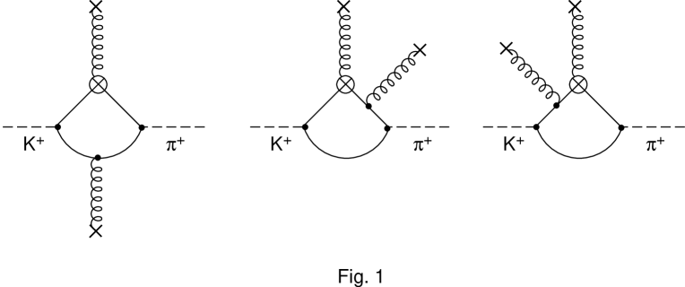
Figure 1: The relevant diagrams for the $K^{+}\rightarrow\pi^{+}$ transition induced by $Q_{11}$. The circled cross indicates the operator insertion.

where $k$ is the off-shell momentum. Matching eq. (3.8) with the corresponding quark loop amplitude, represented by the diagrams in Fig. 1, leads to

$$G_{\underline{8}}^{(4)}(Q_{11})\,=\,-\,\frac{11}{4}\,\langle\overline{q}q\rangle_{G}\,\left(\frac{C_{11}}{16\pi^{2}}\right)\,,$$ (3.9)

where we have used

$$\langle\overline{q}q\rangle_{G}\;\;\equiv\;\;-\frac{1}{12M}\,\langle\frac{\alpha_{s}}{\pi}GG\rangle\ ,$$ (3.10)

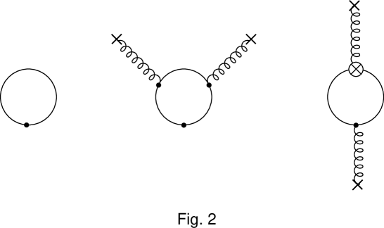
Figure 2: The diagrams for the bare quark condensate, its gluon-condensate correction, and the mixed condensate $g_{s}\langle\overline{q}\sigma\cdot Gq\rangle$. The circled cross indicates the insertion of $Q_{11}$.

which represents the two-gluon condensate contribution to the quark condensate (second diagram in Fig. 2). Diagrams analogous to those in Fig. 1 with the two meson lines entering at the same point do not contribute to momentum dependent terms, and are disregarded. In Table 1 we show the values of $\langle\overline{q}q\rangle_{G}$ as a function of $M$. For the gluon condensate we have taken the central value of the lattice evaluation $\langle\frac{\alpha_{s}}{\pi}GG\rangle=(460\pm 20)^{4}$ MeV⁴ [25]. The entries shown can be scaled accordingly for other values of the gluon condensate.

Having determined $G_{\underline{8}}^{(4)}(Q_{11})$ from the $K\rightarrow\pi$ transition, we can deduce the $K\rightarrow 2\pi$ amplitude from the chiral structure of ${\cal{L}}^{(4)}(Q_{11})$:

$${\cal A}(K^{0}\rightarrow\pi^{+}\pi^{-};Q_{11})\,=\,\frac{\sqrt{2}}{f^{3}}\,(m_{s}-m_{d})\,m_{\pi}^{2}\,\,G_{\underline{8}}^{(4)}(Q_{11})\;,$$ (3.11)

Even though the coefficient in ${\cal{L}}^{(4)}(Q_{11})$ is large, the $Q_{11}$ contribution to $K\rightarrow 2\pi$ is small because of the factor $m_{\pi}^{2}$ (in place of $m_{K}^{2}$ obtained for $Q_{6}$). The modest role played by $Q_{11}$ in $\varepsilon^{\prime}/\varepsilon$ comes therefore from this kinematical suppression rather than from its contribution being NLO in the chiral expansion.

4 Next-to-leading order bosonization of $Q_{6}$

The bosonization of $Q_{6}$ follows basically the same line as for $Q_{11}$ in the preceding section. The standard expression (obtained from eq. (1.2) by a Fierz transformation)

$$Q_{6}\,=\,-\,8\,\sum_{q}(\overline{s}_{L}q_{R})\,(\overline{q}_{R}d_{L})\;,$$ (4.1)

can be rewritten in the rotated picture as

$$Q_{6}\,=\,-\,8\,(F_{(-)})_{\alpha\beta}\,(\overline{\cal{Q}}_{L})_{\alpha}({\cal{Q}}_{R})_{\delta}(\overline{\cal{Q}}_{R})_{\delta}({\cal{Q}}_{L})_{\beta}\,,$$ (4.2)

where $F_{(-)}\;=\,\xi\,\lambda_{-}\xi^{\dagger}$, and the greek letters are flavor indices. Thus, likewise to ${\cal{L}}^{(4)}(Q_{11})$, the chiral representation of $Q_{6}$ to leading order can be written as

$${\cal{L}}^{(2)}(Q_{6})\,\sim\,\mathop{\mbox{Tr}}\,\Bigl{[}F_{(-)}{\cal{A}}_{\mu}\,{\cal{A}}^{\mu}\Bigr{]}\,,$$ (4.3)

which by means of eq. (2.13) can be written in the same familiar form as the other $|\Delta S=1|$ octet operators $O(p^{2})$ [26]:

$${\cal{L}}^{(2)}_{\Delta S=1}\,=\,G^{(2)}_{\underline{8}}(Q_{6})\,\mathop{\mbox{Tr}}\,\Bigl{(}\lambda_{-}D^{\mu}\Sigma^{\dagger}D_{\mu}\Sigma\Bigr{)}\,,$$ (4.4)

where $G^{(2)}_{\underline{8}}(Q_{6})$ is the most important component. The term in eq. (4.4) gives rise to the amplitudes

$${\cal A}(K^{+}\rightarrow\pi^{+};\,Q_{6}) = \frac{2i}{f^{2}}\ k^{2}\ G_{\underline{8}}^{(2)}(Q_{6})\,,$$ (4.5)

$${\cal A}(K^{0}\rightarrow\pi^{+}\pi^{-};\,Q_{6}) = \frac{\sqrt{2}}{f^{3}}\Bigl{[}m_{K}^{2}-m_{\pi}^{2}\Bigr{]}\,G_{\underline{8}}^{(2)}(Q_{6})\,.$$ (4.6)

Now, we want to find the bosonization of $Q_{6}$ to the same order as ${\cal{L}}^{(4)}(Q_{11})$ in the preceding section. That is, the bosonized operator has to contain a mass insertion in addition to what is already included in ${\cal{L}}^{(2)}(Q_{6})$. The QCD mass lagrangian can be written as

$${\cal{L}}_{\ \mbox{\scriptsize mass}}\,=\,-\,\left[\overline{q}_{R}\,{\cal{M}}_{q}\,q_{L}\,+\,\overline{q}_{L}\,{\cal{M}}_{q}^{\dagger}\,q_{R}\right]\;,$$ (4.7)

which can be transformed to the form ${\cal{L}}_{\ \mbox{\scriptsize mass}}\,=\,-\,\overline{{\cal{Q}}}\widetilde{M}_{q}{\cal{Q}}$, where

$$\widetilde{M}_{q}\;\equiv\;\xi^{\dagger}\,{\cal{M}}_{q}\xi^{\dagger}\,L\;+\;\xi\,{\cal{M}}_{q}^{\dagger}\,\xi\,R\,.$$ (4.8)

Therefore, a possible NLO representation of $Q_{6}$ is given by

$${\cal{L}}^{(4)}(Q_{6})\,\sim\,\mathop{\mbox{Tr}}\,\Bigl{[}F_{(-)}\,{\cal{A}}_{\mu}\,\widetilde{M}_{q}^{X}\,{\cal{A}}^{\mu}\Bigr{]}\,,$$ (4.9)

with the addition of two other terms, where the quantities within the trace are permuted. In eq. (4.9) $\widetilde{M}_{q}^{X}$ represents some part of $\widetilde{M_{q}}$ (i.e. $X=R,L,V,A$). Using eq. (2.13), we obtain three different $CPS$-symmetric terms:

$${\cal{L}}^{(4)}_{E}(Q_{6})\;=\;G_{E}^{(4)}(Q_{6})\,\mathop{\mbox{Tr}}\,\Bigl{[}\left(\Sigma^{\dagger}\,{\cal{M}}_{q}\lambda_{-}\,+\;\lambda_{-}{\cal{M}}_{q}^{\dagger}\,\Sigma\right)\,D^{\mu}\Sigma^{\dagger}D_{\mu}\Sigma\Bigr{]}\;,$$ (4.10)

$${\cal{L}}^{(4)}_{H}(Q_{6})\;=\;G_{H}^{(4)}(Q_{6})\,\mathop{\mbox{Tr}}\,\Bigl{[}\left(\lambda_{-}\,\Sigma^{\dagger}\,{\cal{M}}_{q}\,+\;{\cal{M}}_{q}^{\dagger}\,\Sigma\,\lambda_{-}\right)\,D^{\mu}\Sigma^{\dagger}D_{\mu}\Sigma\Bigr{]}\;,$$ (4.11)

$${\cal{L}}^{(4)}_{K}(Q_{6})\;=\;G_{K}^{(4)}(Q_{6})\,\mathop{\mbox{Tr}}\,\Bigl{[}\left(\Sigma\,{\cal{M}}_{q}^{\dagger}\;+\;{\cal{M}}_{q}\,\Sigma^{\dagger}\right)\,D^{\mu}\Sigma\,\lambda_{-}\,D_{\mu}\Sigma^{\dagger}\Bigl{]}\,.$$ (4.12)

These three terms are in fact linear combinations of those given in ref. [15] (again we have discarded subleading terms which are the product of two traces). Note that the last term is not immediately obtained by inserting $\lambda_{-}$ within the trace in ${\cal{L}}^{(4)}_{s}$; in order to obtain (4.12), one has to use $D^{\mu}\Sigma\,=\,-\Sigma\,(D_{\mu}\Sigma^{\dagger})\,\Sigma$ and $1=\Sigma\,\Sigma^{\dagger}\rightarrow\Sigma\,\lambda_{-}\,\Sigma^{\dagger}$. In the case of ${\cal{L}}^{(4)}(Q_{11})$ it was sufficient to calculate the $K\rightarrow\pi$ transition induced by $Q_{11}$ to determine the unique coefficient. Here we have to find three coefficients instead.

The $K\rightarrow\pi$ transitions are given by:

$${\cal A}(K^{+}\rightarrow\pi^{+})_{E,H}\,=\,\frac{2i}{f^{2}}\,(m_{s}+m_{d})\,k^{2}\,G_{E,H}^{(4)}\;,$$ (4.13)

$${\cal A}(K^{+}\rightarrow\pi^{+})_{K}\,=\,\frac{4i}{f^{2}}\,m_{u}\,k^{2}\,G_{K}^{(4)}\,,$$ (4.14)

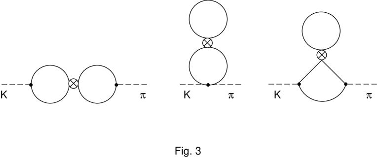
Figure 3: The relevant diagrams for the $K\rightarrow\pi$ transition induced by $Q_{6}$. The circled cross indicates the $Q_{6}$ insertion.

which show that $G_{E}^{(4)}(Q_{6})$ and $G_{H}^{(4)}(Q_{6})$ cannot be distinguished at this level (to consider other off-shell meson-to-meson transitions does not solve the problem). Thus, from the calculation of $K\rightarrow\pi$ transitions (see Fig. 3 for the relevant diagrams) we can at most determine $G_{K}^{(4)}(Q_{6})$ and the sum $[G_{E}^{(4)}(Q_{6})+G_{H}^{(4)}(Q_{6})]$. We therefore have also to consider the $K\rightarrow 2\pi$ amplitudes at the quark level, and match them with the chiral lagrangian results:

$${\cal A}(K^{0}\rightarrow\pi^{+}\pi^{-})_{E} = \frac{\sqrt{2}}{f^{3}}\,(m_{s}-m_{d})\,m_{\pi}^{2}\,G_{E}^{(4)}\,,$$ (4.15)

$${\cal A}(K^{0}\rightarrow\pi^{+}\pi^{-})_{H} = \frac{\sqrt{2}}{f^{3}}\,\left[(m_{s}+m_{d})\,(m_{K}^{2}-m_{\pi}^{2})\right.$$ (4.16)

$$\!\!\!\!+\left.(m_{u}+m_{d})\,(m_{K}^{2}-m_{\pi}^{2})+(m_{u}-m_{d})\,m_{\pi}^{2}\right]G_{H}^{(4)}\,,$$

$${\cal A}(K^{0}\rightarrow\pi^{+}\pi^{-})_{K} = \frac{2\sqrt{2}}{f^{3}}\,\left[(m_{d}-m_{u})\,m_{\pi}^{2}+m_{d}\,(m_{K}^{2}-m_{\pi}^{2})\,\right]G_{K}^{(4)}\,.$$ (4.17)

From eq. (4.16) it appears that in order to determine $G_{H}^{(4)}(Q_{6})$ by calculating quark loops for $K\rightarrow 2\pi$, we may keep the $m_{s}m_{K}^{2}$ terms only. Moreover, if the coefficients $G^{(4)}_{E,H,K}(Q_{6})$ are of the same order of magnitude, the term ${\cal{L}}^{(4)}_{H}$ will be the most important one.

To determine the coefficients $G_{E,H,K}^{(4)}(Q_{6})$, we calculate the $K\rightarrow\pi$ and $K\rightarrow 2\pi$ amplitudes due to $Q_{6}$ within the $\chi$QM. For the $K\rightarrow\pi$ transitions, in the leading factorizable limit, we obtain:

$$\langle\pi^{+}|Q_{6}|K^{+}\rangle\, = 2\,\langle\pi^{+}|\overline{u}\gamma_{5}d|0\rangle\langle 0|\overline{s}\gamma_{5}u|K^{+}\rangle$$ (4.18)

$$-2\left[\langle 0|\overline{d}d|0\rangle+\langle 0|\overline{s}s|0\rangle\right]\langle\pi^{+}|\overline{s}d|K^{+}\rangle$$

and for $K\rightarrow 2\pi$:

$$\langle\pi^{+}\pi^{-}|Q_{6}|K^{0}\rangle\, = 2\,\langle\pi^{+}|\overline{u}\gamma_{5}d|0\rangle\langle\pi^{-}|\overline{s}u|K^{0}\rangle-2\langle\pi^{+}\pi^{-}|\overline{d}d|0\rangle\langle 0|\overline{s}\gamma_{5}d|K^{0}\rangle$$ (4.19)

$$+2\left[\langle 0|\overline{s}s|0\rangle\,-\,\langle 0|\overline{d}d|0\rangle\right]\,\langle\pi^{+}\pi^{-}|\overline{s}\gamma_{5}d|K^{0}\rangle\,.$$

These equations contain some building blocks which we calculate within the $\chi$QM. The quark condensate (Fig. 2) with mass insertions included is given by

$$\langle\overline{q}q\rangle\,=\,\langle\overline{q}q\rangle^{(0)}\,+\,\frac{1}{2M}(m_{s}+m_{u})\left[\langle\overline{q}q\rangle^{(0)}\ +\ Mff_{\pi}^{(0)}\right]\ +\ \langle\overline{q}q\rangle_{G}\,.$$ (4.20)

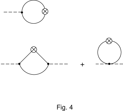
Figure 4: Building blocks for the hadronic matrix elements. The diagram on the top corresponds to $\langle 0|\,\overline{s}\gamma_{5}u\,|K^{+}(k)\rangle$, whereas the two diagrams on the bottom contribute to $\langle\pi^{+}(p)|\,\overline{s}d\,|K^{+}(k)\rangle$. The circled cross indicates the quark current (or density) insertion.

where the last term represents the two-gluon condensate contribution (see eq. (3.10)). As for the diagrams in Fig. 4, in the naive dimensional regularization (NDR) scheme (anti-commuting $\gamma_{5}$ in $d\neq 4$), we obtain:

$$\langle 0|\,\overline{s}\gamma_{5}u\,|K^{+}(k)\rangle_{\mbox{\scriptsize NDR}} = i\sqrt{2}\;\left[\frac{\langle\overline{q}q\rangle^{(0)}}{f}-k^{2}\,\frac{f_{\pi}^{(0)}}{2M}\right.$$ (4.21)

$$\left.+(m_{s}+m_{u})\left(f_{\pi}^{(0)}+3\,f\frac{k^{2}}{\Lambda_{\chi}^{2}}\right)\right]\,,$$

$$\langle\pi^{+}(p_{+})|\,\overline{s}d\,|K^{+}(k)\rangle_{\mbox{\scriptsize NDR}}\, = \,-\frac{\langle\overline{q}q\rangle^{(0)}}{f^{2}}+\frac{3M}{2\Lambda_{\chi}^{2}}P^{2}\,+\,\frac{q^{2}}{2M}\left(f_{+}\,\,-3\,\frac{M^{2}}{\Lambda_{\chi}^{2}}\right)$$ (4.22)

$$-\,m_{s}\left[\left(f_{+}-6\,\frac{M^{2}}{\Lambda_{\chi}^{2}}\right)-\frac{q^{2}+q\cdot P}{2\Lambda_{\chi}^{2}}\right]$$

$$-2\,m_{u}\left(f_{+}+3\,\frac{k^{2}}{\Lambda_{\chi}^{2}}\right)\,,$$

where $q=k-p_{+}$ and $P=k+p_{+}$, while $f_{+}\equiv f^{(0)}_{\pi}/f=1$ can be identified with the vector form factor at zero momentum transfer $q$. Similarly, in the ’t Hooft–Veltman (HV) scheme (commuting $\gamma_{5}$ in $d\neq 4$), we find:

$$\langle 0|\,\overline{s}\gamma_{5}u\,|K^{+}(k)\rangle_{\mbox{scriptsize HV}} = \langle 0|\,\overline{s}\gamma_{5}u\,|K^{+}(k)\rangle_{\mbox{\scriptsize NDR}}$$ (4.23)

$$+i\sqrt{2}\ f\ \left[12\,\frac{M^{3}}{\Lambda_{\chi}^{2}}\left(1-\frac{k^{2}}{6M^{2}}\right)\right.$$

$$\left.+12\,(m_{s}+m_{u})\frac{M^{2}}{\Lambda_{\chi}^{2}}\right]\,,$$

$$\langle\pi^{+}(p_{+})|\,\overline{s}d\,|K^{+}(k)\rangle_{\mbox{\scriptsize HV}} = \langle\pi^{+}(p_{+})|\,\overline{s}d\,|K^{+}(k)\rangle_{\mbox{\scriptsize NDR}}-24\,\frac{M^{3}}{\Lambda_{\chi}^{2}}\,.$$ (4.24)

In eqs. (4.21)–(4.24) we have introduced the chiral symmetry-breaking scale

$$\Lambda_{\chi}\equiv 2\pi\ \sqrt{\frac{6}{N_{c}}}\ f=0.83-1.0\ \mbox{GeV}\,,$$ (4.25)

where the given range corresponds to assigning to $f$ the numerical values of $f_{\pi}$ and $f_{K}$, as indication of $SU(3)$-breaking effects. Notice that identifying $f^{(0)}_{\pi}=f$ in eq. (2.5) leads to $f\sim\sqrt{N_{c}}$, which makes $\Lambda_{\chi}$ independent of $N_{c}$. As a consequence, the $N_{c}$ dependence of eqs. (4.21)–(4.24) resides entirely in $f$ and $\langle\overline{q}q\rangle\sim N_{c}$.

The terms containing current quark masses are obtained from mass-insertions due to ${\cal{L}}_{mass}$ in eq. (4.7) in the various quark loop diagrams in Fig. 4. We have discarded terms proportional to $m_{d}$ because they are not needed in determining $G_{E,H,K}^{(4)}(Q_{6})$. The matrix element $\langle\pi^{+}(p_{+})|\overline{u}\gamma_{5}d|0\rangle$ is obtained from $\langle 0|\overline{s}\gamma_{5}u|K^{+}(k)\rangle$ by obvious substitutions, while $\langle\pi^{+}(p_{+})\pi^{-}(p_{-})|\overline{d}d|0\rangle$ (where $p_{+}+p_{-}=k$) can be derived from eq. (4.22) and (4.24) by crossing ($k\rightarrow-p_{-}$). Finally, $\langle\pi^{+}\pi^{-}|\overline{s}\gamma_{5}d|K^{0}\rangle$ is zero to this order [27, 28]. Notice that these expressions are more general than those given by other authors [27, 28], because our results are not based on the divergence of the on-shell current.

By using these matrix elements, we find that the constant term for the $Q_{6}-$induced $K\rightarrow\pi$ transition vanishes as it should according to chiral symmetry [28, 29, 30]. This cancellation is exact in NDR; in the HV, it holds only up to terms of order $1/\Lambda_{\chi}^{4}$, a warning about the relevance of higher-order loop effects. A typical example of such a high order contribution would be any diagram in Fig. 3 with an extra meson line connecting the two quark loops. For consistency, we will always drop terms of order $1/\Lambda_{\chi}^{4}$ or higher in all numerical estimates.

In the NDR scheme, neglecting current quark masses which would amount to a correction $\leq 10\%$, the LO coefficient for the $Q_{6}$ matrix element is therefore

$$G_{\underline{8}}^{(2)}(Q_{6})=C_{6}\,\frac{2f^{2}}{M}\langle\overline{q}q\rangle^{(0)}\ \left(f_{+}-6\,\frac{M^{2}}{\Lambda_{\chi}^{2}}\right)\,,$$ (4.26)

while the result in the HV scheme is

$$G_{\underline{8}}^{(2)}(Q_{6})=C_{6}\ \frac{2f^{2}}{M}\langle\overline{q}q\rangle^{(0)}\ \left[f_{+}-2\,\frac{M^{2}}{\Lambda_{\chi}^{2}}+12\frac{M^{3}f^{2}}{\langle\overline{q}q\rangle^{(0)}\Lambda_{\chi}^{2}}\left(1+4\,\frac{M^{2}}{\Lambda_{\chi}^{2}}\right)\right]\,.$$ (4.27)

Then the relation

$$G_{\underline{8}}^{(2)}(Q_{6})\equiv-16\,C_{6}\,\frac{L_{5}}{f^{2}}\left[\langle\overline{q}q\rangle^{(0)}\right]^{2}\,,$$ (4.28)

defines the NLO chiral parameter $L_{5}$ in agreement with refs. [7, 8]. In passing, let us remark that the leading non-zero matrix element of $Q_{6}$ is next-to-leading in the framework of the chiral perturbation theory since it is proportional to the coefficient $L_{5}$ of $\mathop{\mbox{Tr}}\,[(\Sigma^{\dagger}\,{\cal{M}}_{q}\,+\;{\cal{M}}_{q}^{\dagger}\,\Sigma)\,D^{\mu}\Sigma^{\dagger}D_{\mu}\Sigma]$ in ${\cal{L}}^{(4)}_{s}$.

In the $\chi$QM, to order $M^{2}/\Lambda_{\chi}^{2}$, we find

$$L_{5}^{\mbox{\scriptsize NDR}}=-\frac{f^{4}}{8M\langle\overline{q}q\rangle}\left(f_{+}-6\,\frac{M^{2}}{\Lambda_{\chi}^{2}}\right)\,,$$ (4.29)

as in ref. [8], and

$$L_{5}^{\mbox{\scriptsize HV}}=-\frac{f^{4}}{8M\langle\overline{q}q\rangle}\left(f_{+}-2\,\frac{M^{2}}{\Lambda_{\chi}^{2}}+12\frac{M^{3}f^{2}}{\langle\overline{q}q\rangle^{(0)}\Lambda_{\chi}^{2}}\right)\,,$$ (4.30)

both sensitive functions of $M$. Let us remark that for

$$L_{5}=\frac{1}{4}\,\frac{f^{2}_{\pi}}{\Lambda_{\chi}^{2}}\left(\frac{f_{\pi}}{f_{K}}\right)^{4}$$ (4.31)

eq. (4.28) used in eq. (4.6) gives the usual $1/N_{c}$ matrix element [4]. In that scheme we therefore have

$$L_{5} = 1.4\times 10^{-3}\qquad\qquad\qquad\qquad\mbox{for}\quad\Lambda_{\chi}=0.83\>\mbox{GeV}$$

$$L_{5} = 1.0\times 10^{-3}\qquad\qquad\qquad\qquad\mbox{for}\quad\Lambda_{\chi}=1.0\>\mbox{GeV}\,.$$ (4.32)

A scale-dependent value for $L_{5}$ can be extracted in $\chi$PT from the ratio $f_{K}/f_{\pi}$ where one finds [31]

$$\mbox{$L_{5}(m_{\rho})=(1.4\pm 0.5)\times 10^{-3}$}\ ,$$ (4.33)

which we use for comparison with eqs. (4.29)–(4.31).

In Table 2 we have collected the results of the $\chi$QM predictions for $L_{5}$ in the two schemes as we vary $M$. A constraint of approximately 3$\sigma$ from the central value in eq. (4.33) gives

$$140\ \mbox{MeV}\ \raisebox{-1.72218pt}{\hbox to0.0pt{$\sim$\hss}}\raisebox{1.72218pt}{$<$}\ M\ \raisebox{-1.72218pt}{\hbox to0.0pt{$\sim$\hss}}\raisebox{1.72218pt}{$<$}\ 340\ \mbox{MeV}\,,$$ (4.34)

where we have taken for the scale dependent quark condensate the expression in eq. (5.12), and assumed a perturbative running for $\mu\geq 1$ GeV. Recall however that for $M>300$ MeV $M^{4}/\Lambda_{\chi}^{4}$ corrections become relevant and may affect the smaller values of $L_{5}$ listed in Table 2.

Moving on to the NLO contributions, by using eqs. (4.15)–(4.17) we find in the NDR scheme:

$$G_{E}^{(4)}(Q_{6}) = -\,2\,C_{6}\,\langle\overline{q}q\rangle^{(0)}\left(\frac{f^{2}}{\Lambda_{\chi}^{2}}-\frac{3f^{4}}{2M\langle\overline{q}q\rangle^{(0)}}\right)\,,$$ (4.35)

$$G_{K}^{(4)}(Q_{6}) = 3\ C_{6}\,\langle\overline{q}q\rangle^{(0)}\left(\frac{f^{2}}{\Lambda_{\chi}^{2}}+\frac{f^{4}f_{+}^{2}}{6M\langle\overline{q}q\rangle^{(0)}}\right)\,,$$ (4.36)

whereas in the HV scheme:

$$G_{E}^{(4)}(Q_{6}) = -\,2\,C_{6}\,\langle\overline{q}q\rangle^{(0)}\left[\frac{f^{2}}{\Lambda_{\chi}^{2}}-6\frac{M^{3}f^{4}}{\langle\bar{q}q\rangle^{(0)}\Lambda_{\chi}^{4}}-\frac{5f^{4}}{M\langle\bar{q}q\rangle^{(0)}}\left(1+12\frac{M^{2}}{\Lambda_{\chi}^{2}}\right)\right]\,,$$ (4.37)

$$G_{K}^{(4)}(Q_{6}) = 3\ C_{6}\,\langle\overline{q}q\rangle^{(0)}\left[\frac{f^{2}}{\Lambda_{\chi}^{2}}\left(1+12\frac{M^{3}f^{4}}{\langle\bar{q}q\rangle^{(0)}\Lambda_{\chi}^{4}}\right)\right.$$ (4.38)

$$\hskip 71.13188pt\left.-\frac{f^{4}}{6M\langle\bar{q}q\rangle^{(0)}}\left(f_{+}+4\frac{M^{2}}{\Lambda_{\chi}^{2}}\right)\left(f_{+}+12\frac{M^{2}}{\Lambda_{\chi}^{2}}\right)\right]\,.$$

The most important contribution to $K\rightarrow 2\pi$ comes from the third coefficient $G_{H}^{(4)}(Q_{6})$, since the corresponding amplitude is enhanced by a factor $m_{K}^{2}/m_{\pi}^{2}$ compared to the other two (see eqs. (4.15)–(4.17)). In the NDR scheme we find:

$$G_{H}^{(4)}(Q_{6})\ \ =\ \ -7\,C_{6}\,\langle\overline{q}q\rangle^{(0)}\left[\frac{f^{2}}{\Lambda_{\chi}^{2}}-\frac{f^{4}}{7M\langle\bar{q}q\rangle^{(0)}}\left(f_{+}-6\frac{M^{2}}{\Lambda_{\chi}^{2}}\right)\right]\,,$$ (4.39)

whereas the HV result is:

$$G_{H}^{(4)}(Q_{6}) = -7\,C_{6}\,\langle\overline{q}q\rangle^{(0)}\left[\frac{f^{2}}{\Lambda_{\chi}^{2}}+\frac{156}{7}\frac{M^{3}f^{4}}{\langle\bar{q}q\rangle^{(0)}\Lambda_{\chi}^{4}}\right.$$ (4.40)

$$\hskip 71.13188pt\left.-\frac{f^{4}}{7M\langle\bar{q}q\rangle^{(0)}}\left(f_{+}-6\frac{M^{2}}{\Lambda_{\chi}^{2}}\right)\left(1+12\frac{M^{2}}{\Lambda_{\chi}^{2}}\right)\right]\,.$$

Recently an NLO analysis of the hadronic matrix elements $Q_{1-10}$ has appeared [32], which makes use of effective scalar-meson exchange. The result of ref. [32] for the operator $Q_{6}$ does not contain terms corresponding to ${\cal{L}}^{(6)}_{s}$ (with two derivatives and current masses squared), which contribute to eqs. (4.15)–(4.17).

We see that $G_{E,H,K}^{(4)}(Q_{6})$ are formally suppressed by terms proportional to either $f^{2}/\Lambda_{\chi}^{2}$ or $f^{4}/(M\langle\bar{q}q\rangle^{(0)})$ with respect to $G^{(4)}(Q_{11})$. However, because of the numerical factors in front, the NLO $G^{(4)}(Q_{6})$ coefficients turn out to be numerically of the same size as $G^{(4)}(Q_{11})$. Since the amplitude due to ${\cal{L}}^{(4)}(Q_{11})$ is effectively suppressed by a factor $m_{\pi}^{2}/m_{K}^{2}$ with respect to the amplitudes obtained from ${\cal{L}}^{(2)}(Q_{6})$ and ${\cal{L}}_{H}$, the contribution of $Q_{11}$ to $\varepsilon^{\prime}/\varepsilon$ turns out to be generally more than one order of magnitude smaller than these NLO corrections (see Table 3). The same can be said of other subleading operators such as $Q_{3}$, $Q_{5}$ and $Q_{7}$ (see eq. (6.2) below for the definitions, and Tables 7–9).

In Table 3 we have reported the weights of the NLO matrix elements of $Q_{6}$ and $Q_{11}$ relative to the LO $Q_{6}$ amplitude, as computed in the $\chi$QM. These estimates are robust as they do not sensibly depend on the detailed values of $\Lambda_{QCD}$ and $\Lambda_{\chi}$.

5 Scheme dependence of $\langle Q_{6}\rangle_{\underline{8}}$ and $\langle Q_{8}\rangle_{\underline{27}}$

The Wilson coefficients computed by means of the renormalization group equations depend, at the NLO, on whether the NDR or the HV prescriptions are used in treating $\gamma_{5}$ in $d$ dimension. At the same time, the matrix elements of the relevant operators do not have any scheme dependence, at least if computed by $1/N_{c}$ techniques. As a consequence, there remains a $\gamma_{5}$-scheme dependence which increases the uncertainties in the final result. The discrepancy between the HV and NDR result goes from $30\%\>(\Lambda_{QCD}=200$ MeV) to $40\%\>(\Lambda_{QCD}=400$ MeV) at $m_{t}=130$ MeV, becoming much worse in the “superweak” regime at $m_{t}=170$ GeV, where it goes from $70\%\>(\Lambda_{QCD}=200$ MeV) to $80\%\>(\Lambda_{QCD}=400$ MeV) [2].

A potentially nice feature of the $\chi$QM is that it makes it possible to compute also the matrix elements in both schemes. In eqs. (4.26)–(4.27) we have computed the matrix element for the operators $Q_{6}$ to the leading order in the chiral expansion. The next most relevant contribution comes from the electroweak penguin operator $Q_{8}$ (eq. (1.3)). This operator can be written as

$$Q_{8}=\frac{3}{2}e_{d}\cdot Q_{6}\ \ +\ \ \frac{3}{2}(e_{u}-e_{d})\ \overline{s}_{\alpha}\gamma_{\mu}(1-\gamma_{5})d_{\beta}\ \ \overline{u}_{\beta}\gamma^{\mu}(1+\gamma_{5})u_{\alpha}\ ,$$ (5.1)

where $e_{u}=-2e_{d}=2/3$, so as to obtain

$$\langle\pi^{+}\pi^{-}|Q_{8}|K^{0}\rangle_{\underline{8}}\ \ =\ \ \langle\pi^{0}\pi^{0}|Q_{8}|K^{0}\rangle_{\underline{8}}\ \ =\ \ -\frac{1}{2}\ \langle\pi^{+}\pi^{-}|Q_{6}|K^{0}\rangle_{\underline{8}}\ ,$$ (5.2)

and, after a Fierz rearrangement and factorization,

$$\langle\pi^{+}\pi^{-}|Q_{8}|K^{0}\rangle_{\underline{27}} = 3\ \langle\pi^{+}|\bar{u}\gamma_{5}d|0\rangle\langle\pi^{-}|\bar{s}u|K^{0}\rangle\ ,$$ (5.3)

$$\langle\pi^{0}\pi^{0}|Q_{8}|K^{0}\rangle_{\underline{27}} = 0\ .$$ (5.4)

The leading order amplitude corresponding to eq. (5.3) is therefore given by

$${\cal A}(K^{0}\rightarrow\pi^{+}\pi^{-};\,Q_{8})_{\underline{27}}\ \ =\ \ C_{8}\frac{3\sqrt{2}}{f^{3}}\Bigl{[}\langle\overline{q}q\rangle^{(0)}\Bigr{]}^{2}$$ (5.5)

in the NDR scheme, and

$${\cal A}(K^{0}\rightarrow\pi^{+}\pi^{-};\,Q_{8})_{\underline{27}} = C_{8}\frac{3\sqrt{2}}{f^{3}}\Bigl{[}\langle\overline{q}q\rangle^{(0)}\Bigr{]}^{2}\times$$ (5.6)

$$\hskip 28.45274pt\left(1+12\frac{M^{3}f^{2}}{\langle\overline{q}q\rangle^{(0)}\Lambda_{\chi}^{2}}\right)\left(1+24\frac{M^{3}f^{2}}{\langle\overline{q}q\rangle^{(0)}\Lambda_{\chi}^{2}}\right)$$

in the HV scheme. In eqs. (5.5)–(5.6) we have kept only the leading momentum-independent terms. The momentum-dependent corrections are at the 10% level.

In a toy model for $\varepsilon^{\prime}/\varepsilon$ in which we use the full mixing to determine the Wilson coefficients, but keep only the contribution of the two leading operators $Q_{6}$ (for the $I=0$ amplitude) and $Q_{8}$ (for $I=2$), we can compare the scheme dependence in the $1/N_{c}$ approach—where it only appears in the Wilson coefficients—and in the $\chi$QM, for different choices of $M$.

We have taken the Wilson coefficients at $\mu=$ 1 GeV ($\mu=$ 1.4 GeV) for $m_{t}=170$ GeV and multiplied them by the corresponding matrix elements, according to eq. (6.5) in the next section. We have used

$$\langle 2\pi,\>I=0|\,Q_{i}\,|K^{0}\rangle = \sqrt{\frac{2}{3}}\>\langle\pi^{+}\pi^{-}|Q_{i}|K^{0}\rangle\ \ +\ \ \sqrt{\frac{1}{6}}\>\langle\pi^{0}\pi^{0}|Q_{i}|K^{0}\rangle\ ,$$ (5.7)

$$\langle 2\pi,\>I=2|\,Q_{i}\,|K^{0}\rangle = \sqrt{\frac{1}{3}}\>\Bigl{[}\langle\pi^{+}\pi^{-}|Q_{i}|K^{0}\rangle\ \ -\ \ \langle\pi^{0}\pi^{0}|Q_{i}|K^{0}\rangle\Bigr{]}\ .$$ (5.8)

In our case

$$\langle 2\pi,\>I=0|\,Q_{6}\,|K^{0}\rangle = \sqrt{\frac{3}{2}}\>\langle\pi^{+}\pi^{-}|Q_{6}|K^{0}\rangle_{\underline{8}}\,,$$ (5.9)

$$\langle 2\pi,\>I=2|\,Q_{8}\,|K^{0}\rangle = \sqrt{\frac{1}{3}}\>\langle\pi^{+}\pi^{-}|Q_{8}|K^{0}\rangle_{\underline{27}}\,.$$ (5.10)

Consistently to our approximation, we neglect the $I=0$ contribution of $Q_{8}$:

$$\langle 2\pi,\>I=0|\,Q_{8}\,|K^{0}\rangle\ \ =\ -\ \frac{1}{2}\ \langle 2\pi,\>I=0|\,Q_{6}\,|K^{0}\rangle\ +\ \sqrt{\frac{2}{3}}\>\langle\pi^{+}\pi^{-}|Q_{8}|K^{0}\rangle_{\underline{27}}\ ,$$ (5.11)

since it is suppressed in $\varepsilon^{\prime}/\varepsilon$ by a factor $\sim 1/20$ ($\Delta I=1/2$ rule) with respect to the $I=2$ contribution of eq. (5.10). Notice that, at the zeroth order in momentum expansion, $\langle\pi^{+}\pi^{-}|Q_{6}|K^{0}\rangle=0$ and, as a consequence, the last term in eq. (5.11) is leading.

The matrix elements in the $\chi$QM are computed using the scale-dependent quark condensate

$$\langle\overline{q}q\rangle(\mu)=-\frac{f_{K}^{2}m_{K}^{2}}{m_{s}(\mu)+m_{d}(\mu)}\,.$$ (5.12)

Following ref. [2], we take $m_{s}(1.4\ \mbox{GeV})=150\ \mbox{MeV}$ and $m_{d}(1.4\ \mbox{GeV})=8.0\ \mbox{MeV}$. The values at other scales are obtained using the NLO evolution of QCD. In particular, for $\Lambda_{QCD}=300\ \mbox{MeV}$ one has $m_{s}(1.0\ \mbox{GeV})=176\ \mbox{MeV}$ and $m_{d}(1.0\ \mbox{GeV})=9.4\ \mbox{MeV}$.

Tables 4 and 5 summarize our findings for different values of $\Lambda^{(4)}_{QCD}$. In using eq. (4.27) and eq. (5.6) we have dropped all terms of order $1/\Lambda_{\chi}^{4}$ for consistency and limited ourselves to values of $M<220$ MeV. As explained in the beginning, we cannot trust our results beyond order $1/\Lambda_{\chi}^{2}$ because we have neglected higher-loop corrections with meson exchange that give $1/\Lambda_{\chi}^{4}$ contributions.

In the range considered, the $\gamma_{5}$-scheme dependence is indeed dramatically reduced. For instance, taking $\Lambda^{(4)}_{QCD}=300$ MeV, $\Delta$—defined as the difference between the HV and the NDR results divided by the HV one—is below $10\%$ for $M\simeq 120-150$ MeV ($\mu=1.4$ GeV) and for $M\simeq 120-170$ MeV ($\mu=1$ GeV), when $\Lambda_{\chi}=830$ MeV; similarly, $\Delta$ is below $10\%$ for $M\simeq 120-180$ MeV ($\mu=1.4$ GeV) and for $M\simeq 150-190$ MeV ($\mu=1$ GeV), when $\Lambda_{\chi}=1$ GeV.

Another, and more restrictive, reading of the same tables puts together all data for different $\Lambda_{QCD}$’s. In this case, stability is achieved for $M\simeq 120-150$ MeV ($\mu=1.4$ GeV) and for $M\simeq 150$ MeV ($\mu=1$ GeV), when $\Lambda_{\chi}=830$ MeV; similarly, $\Delta$ is below $10\%$ for $M\simeq 120-170$ MeV ($\mu=1.4$ GeV) and for $M\simeq 190$ MeV ($\mu=1$ GeV), when $\Lambda_{\chi}=1$ GeV.

To reach values of $M$ larger than its central value and closer to it, we would have to include higher-loop corrections. The preliminary nature of our analysis needs hardly be stressed as only two out of eleven operators have been considered. Even though $Q_{6}$ and $Q_{8}$ induce the most relevant contributions, we expect that a complete estimate of $\varepsilon^{\prime}/\varepsilon$ would result in a more stable range of values of $M$ for which the $\gamma_{5}$-scheme and $\mu$ dependences are reduced. This will also give us confidence on the size of $\varepsilon^{\prime}/\varepsilon$ that is obtained.

6 “NLO” study of $\varepsilon^{\prime}/\varepsilon$ with dipole operators

In this section we discuss the impact of the dipole gluon penguin $Q_{11}$ on present estimates of $\varepsilon^{\prime}/\varepsilon$. The contribution of $Q_{11}$ is given by setting $\langle\bar{q}q\rangle_{G}$ at the rather conservative value of $-(275\,\mbox{MeV})^{3}$ (see Table 1).

Since a satisfactory calculation of $\varepsilon^{\prime}/\varepsilon$ in the $\chi$QM is missing beyond the leading factorizable order (the study is under way), we resort to the $1/N_{c}$ analysis of ref. [2] for the ten traditional operators. We present our results in tables that show a detailed anatomy of the contributions of the different operators, and can be used as reference for future developments.

Because of the many ingredients involved in the calculation of $\varepsilon^{\prime}/\varepsilon$, it is useful to briefly recall the theoretical inputs used. The effective lagrangian for $|\Delta S|=1$ transitions can be written, for $\mu<m_{c}$, as [2]

$${\cal L}_{\Delta S=1}=-\frac{G_{F}}{\sqrt{2}}\lambda_{u}\sum_{i}\Bigl{[}z_{i}(\mu)+\tau y_{i}(\mu)\Bigr{]}Q_{i}(\mu)=\sum_{i}C_{i}(\mu)Q_{i}(\mu)\,.$$ (6.1)

In the previous equation, $\lambda_{i}\equiv V_{id}V^{*}_{is}$, where $V$ is the Kobayashi-Maskawa (KM) matrix, and $\tau\equiv-\lambda_{t}/\lambda_{u}$. The Wilson coefficients $z_{1,2}(\mu)$ run from $m_{W}$ to $m_{c}$ via the corresponding $2\times 2$ sub-block of the $10\times 10$ anomalous-dimension matrices, while $z_{i}(\mu)=0$ for $i=3-10$. From $\mu=m_{c}$ down, as the charm-induced penguins come into play, all $z_{i}(\mu)$ evolve, given the proper matching conditions, with the full anomalous-dimension matrices. The Wilson coefficients $v_{i}(\mu)$ ($y_{i}(\mu)=v_{i}(\mu)-z_{i}(\mu)$) arise at $m_{W}$ due to integration of the $W$ and top quark fields. They coincide with $z_{i}(\mu)$ for $i=1,2$, the information about the top quark being encoded in the $i=3-10$ components.

The list of the effective operators $Q_{i}$ ($i=1-10$) is reported in refs. [2, 3], whose notation we follow closely and where the reader may find a complete discussion of the basic tools. For convenience we report here the ten operators usually considered

$$\begin{array}[]{rcl}Q_{1}&=&\left(\overline{s}_{\alpha}u_{\beta}\right)_{\rm V-A}\left(\overline{u}_{\beta}d_{\alpha}\right)_{\rm V-A}\,,\\[4.30554pt] Q_{2}&=&\left(\overline{s}u\right)_{\rm V-A}\left(\overline{u}d\right)_{\rm V-A}\,,\\[4.30554pt] Q_{3,5}&=&\left(\overline{s}d\right)_{\rm V-A}\sum_{q}\left(\overline{q}q\right)_{\rm V\mp A}\,,\\[4.30554pt] Q_{4,6}&=&\left(\overline{s}_{\alpha}d_{\beta}\right)_{\rm V-A}\sum_{q}(\overline{q}_{\beta}q_{\alpha})_{\rm V\mp A}\,,\\[4.30554pt] Q_{7,9}&=&\frac{3}{2}\left(\overline{s}d\right)_{\rm V-A}\sum_{q}e_{q}\left(\overline{q}q\right)_{\rm V\pm A}\,,\\[4.30554pt] Q_{8,10}&=&\frac{3}{2}\left(\overline{s}_{\alpha}d_{\beta}\right)_{\rm V-A}\sum_{q}e_{q}(\overline{q}_{\beta}q_{\alpha})_{\rm V\pm A}\,,\end{array}$$ (6.2)

where $\alpha$, $\beta$ denote color indices ($\alpha,\beta=1,\ldots,N_{c}$) and $e_{q}$ are quark charges. Color indices for the color singlet operators are omitted. $(V\pm A)$ refer to $\gamma_{\mu}(1\pm\gamma_{5})$. We recall that $Q_{1,2}$ stand for the $W$-induced current–current operators, $Q_{3-6}$ for the QCD penguin operators and $Q_{7-10}$ for the electroweak penguin (and box) ones.

Not all the operators in eq. (6.2) are independent. For $\mu<m_{c}$, having integrated out the charm quark, we have

$$Q_{4} = Q_{3}+Q_{2}-Q_{1}\,,$$

$$Q_{9} = \left(3Q_{1}-Q_{3}\right)/2\,,$$ (6.3)

$$Q_{10} = Q_{2}+\left(Q_{1}-Q_{3}\right)/2\;.$$

Note that these relations hold in the HV scheme, but they may receive additional contributions in other schemes since Fierz transformations have been used in obtaining them.

Together with this basis, which closes under QCD and QED renormalization, one should a-priori consider two additional dimension-five operators: $Q_{11}$ (eq. (1.1)) and

$$Q_{12}\simeq\frac{ee_{d}}{16\pi^{2}}\,m_{s}\>\overline{s}\,\sigma_{\mu\nu}F^{\mu\nu}(1-\gamma_{5})\,d\ ,$$ (6.4)

which account for the magnetic and electric dipole part of, respectively, the QCD and electromagnetic penguin operators. In eq. (6.4) $e_{d}=-1/3$ is the charge of the down quarks.

Actually, in [9] we argued that the hadronic matrix element of the electromagnetic operator (6.4) is negligible and, accordingly, even if we keep the operator in our basis for the Wilson coefficients, we will put its contribution to zero in the end.

Since Im$(\lambda_{u})=0$ according to the standard conventions, the short-distance component of $\varepsilon^{\prime}/\varepsilon$ is determined by the Wilson coefficients $y_{i}$. Following the approach of ref. [2], $y_{1}(\mu)=$ $y_{2}(\mu)=0$ and the effect of $Q_{1,2}$ appears only through the linearly-dependent operators $Q_{4,9,10}$.

The lagrangian in eq. (6.1) yields [2]

$$\frac{\varepsilon^{\prime}}{\varepsilon}=10^{-4}\left[\frac{\mbox{Im}\,\lambda_{t}}{1.7\times 10^{-4}}\right]\Bigl{[}P^{(1/2)}-P^{(3/2)}\Bigr{]}\,,$$ (6.5)

where

$$P^{(1/2)} = r\ \sum y_{i}\,\langle 2\pi,\ I=0|\,Q_{i}\,|K^{0}\rangle\left(1-\Omega_{\eta+\eta^{\prime}}\right)$$ (6.6)

$$P^{(3/2)} = \frac{r}{\omega}\sum y_{i}\,\langle 2\pi,\ I=2|\,Q_{i}\,|K^{0}\rangle\ .$$ (6.7)

We take, as input values for the relevant quantities, the central values given in appendix C of ref. [2]. This allows us to reproduce, in the ten-operator case, the central values of the results given in appendix B of ref. [2]. In particular, we take

$$r=1.7\frac{\omega G_{F}}{2\left|\epsilon\right|\mathop{\mbox{Re}}{A_{0}}}\simeq 594\ \mbox{GeV}^{-3},\qquad\omega=1/22.2\ ,\qquad\Omega_{\eta+\eta^{\prime}}=0.25\ ;$$ (6.8)

$\mathop{\mbox{Im}}{\lambda_{t}}$ is determined from the experimental value of $\varepsilon$ as an interpolating function of $m_{t}$. Its central value, given the KM phase $\delta_{KM}$ in the first or second quadrant, is given by

$$\mathop{\mbox{Im}}{\lambda_{t}}\simeq 2.77\times 10^{-4}\ x_{t}^{-0.365}\ \ \ (\mbox{first quadrant})\ ,$$ (6.9)

and

$$\mathop{\mbox{Im}}{\lambda_{t}}\simeq 2.19\times 10^{-4}\ x_{t}^{-0.47}\ \ \ \mbox{(second quadrant})\ ,$$ (6.10)

where $x_{t}=m_{t}^{2}/m_{W}^{2}$.

The value of the Wilson coefficients $y_{11}$ and $y_{12}$ at the hadronic scale of 1 GeV can be found by means of the renormalization group equations. Denoting generically the vector of Wilson coefficients by $\vec{C}(\mu)$, its scale dependence is governed by

$$\left[\mu\frac{\partial}{\partial\mu}+\beta(g)\frac{\partial}{\partial g}\right]\vec{C}\left(\frac{m_{W}^{2}}{\mu^{2}},g^{2},\alpha\right)\ \ =\ \ \hat{\gamma}^{T}(g^{2},\alpha)\ \vec{C}\left(\frac{m_{W}^{2}}{\mu^{2}},g^{2},\alpha\right)\,,$$ (6.11)

where $\beta(g)$ is the QCD beta function and $\alpha$ the electromagnetic coupling (the running of $\alpha$ is being neglected). At the NLO we have

$$\hat{\gamma}(g^{2},\alpha)=\frac{\alpha_{s}}{4\pi}\left(\hat{\gamma}_{s}^{(0)}+\frac{\alpha_{s}}{4\pi}\hat{\gamma}_{s}^{(1)}\right)+\frac{\alpha}{4\pi}\left(\hat{\gamma}_{e}^{(0)}+\frac{\alpha_{s}}{4\pi}\hat{\gamma}_{se}^{(1)}\right)\ ,$$ (6.12)

where $\hat{\gamma}_{s}^{(0)}$ and $\hat{\gamma}_{e}^{(0)}$ govern the leading QCD and the electromagnetic running respectively. The anomalous-dimension matrices labelled with $(1)$ refer to the NLO running ($O(\alpha^{2})$ effects are neglected).

In order to include all available NLO effects in the evaluation of $\varepsilon^{\prime}/\varepsilon$, we follow the analysis described in ref. [2]. The NLO $10\times 10$ mixing matrices for the operators $Q_{1-10}$ can be found in refs. [2, 3]. Concerning the dipole operators, the leading-order matrix of the strong anomalous dimensions of $Q_{11}$ and $Q_{12}$ and their QCD-induced mixing with $Q_{1-6}$ can be borrowed from the existing calculations for the $b\to s\gamma$ decay [33] (recent discussions are given in ref. [12]). In fact, by replacing $s\to b$ and $d\to s$ in eqs. (6.2)–(6.4) we obtain the operator basis, which should be considered for a complete NLO analysis of $b\to s\gamma$.

While the $10\times 10$ part of the anomalous dimension matrices (6.12) is identical to that used in refs. [2, 3], two extra columns and rows have to be added to represent the mixing of the first ten operators with the two new ones, which takes place first at the two-loop level. We have taken for all two-loop anomalous dimensions the HV scheme results [2, 3]. In this way, no finite additional contributions to the renormalization of $y_{11}$ and $y_{12}$ arise at the various quark thresholds (for a discussion see Misiak in ref. [33] and ref. [11]). The explicit expression of $\hat{\gamma}_{s}^{T}$ is reported for instance in ref. [9]. We just recall that whereas the evolution of the dipole Wilson coefficients $C_{11}$ and $C_{12}$ is substantially affected by the mixings with $Q_{1-10}$, the Wilson coefficients $C_{1-10}$ remain unaffected by the presence of the dipole operators ($Q_{1-10}$ close under QCD and QED renormalization). The two-loop mixings of $Q_{11}$ and $Q_{12}$ with the electroweak penguins ($Q_{7-10}$), not yet given in the literature, can be easily derived from those with the gluon penguins ($Q_{3-6}$). We have verified that their effect on the running of $C_{11}$ and $C_{12}$ is negligible ($<1\%$) and therefore they can be safely set to zero (and, by extension, they can also be set equal to zero in $b\rightarrow s\gamma$).

The complete NLO analysis would require computing, among other things, the three-loop mixings between the dipole operators and the first ten (quite a task!). The lack of knowledge on these entries introduces an uncertainty on the dipole Wilson coefficients which can be as large as 50% (see the analogous discussion for the $b\to s\gamma$ inclusive decay in ref. [12]). However, for what concerns $\varepsilon^{\prime}/\varepsilon$ this uncertainty is diluted over many contributions, and it is certainly not as relevant as our ignorance of the hadronic matrix elements. The results presented here are obtained by adding two rows and two columns of zeros to the $10\times 10$ electromagnetic and NLO anomalous dimension matrices, which can be found in refs. [2, 3]. As a consequence, the contribution of $Q_{11}$ to $\varepsilon^{\prime}/\varepsilon$ takes into account only the “LO” (two-loop) QCD effects.

The expressions for the initial Wilson coefficients $v_{1-10}\,(m_{W})$ can be found for instance in ref. [2]. For what concerns the new coefficients $v_{11,12}\,(m_{W})$ we have

$$v_{11}(m_{W})=-E^{\prime}(m_{t}^{2}/m_{W}^{2})\qquad\mbox{and}\qquad v_{12}(m_{W})=-D^{\prime}(m_{t}^{2}/m_{W}^{2})/e_{d}\,,$$ (6.13)

where

$$E^{\prime}(x) = \frac{3x^{2}}{2(1-x)^{4}}\ln x-\frac{x^{3}-5x^{2}-2x}{4(1-x)^{3}}$$ (6.14)

$$D^{\prime}(x) = \frac{x^{2}(2-3x)}{2(1-x)^{4}}\ln x-\frac{8x^{3}+5x^{2}-7x}{12(1-x)^{3}}\,.$$ (6.15)

In Table 6 we report the HV results we have obtained for $z_{1-12}$ ($\mu=1$ GeV) and $y_{3-12}$ ($\mu=1$ GeV) (recall that $y_{1,2}\,(\mu)=0$) compared with their initial values, for $m_{t}=170$ GeV and for $\Lambda_{QCD}^{(4)}=$ 200, 300 and 400 MeV. We fully agree on the values of the renormalized coefficients for the first ten operators with ref. [2].

Let us remark that the effect of operator mixing induces a renormalization on $v_{11,12}$ ($=y_{11,12}\,+\,z_{11,12}$) which is a factor of 4–5 larger than that induced by multiplicative running alone (which roughly reduces by a factor of two the initial Wilson coefficients).

In order to discuss the effect of the various operators in determining the size of $\varepsilon^{\prime}/\varepsilon$, we need a consistent estimate of the relevant hadronic matrix elements. For the operators $Q_{1-10}$, we follow the strategy of ref. [2] where the various matrix elements are evaluated by means of the $1/N_{c}$ expansion and soft-meson methods. Overall coefficients $B_{i}^{(1/2)}$ and $B_{i}^{(3/2)}\ (i=1-10)$ parametrize our level of ignorance of their normalization scale, scale dependence and the approximation inherent in the method. The matrix elements of $Q_{1}$ and $Q_{2}$ can however be determined phenomenologically from the experimental values of $\mathop{\mbox{Re}}{A_{0}}$ and $\mathop{\mbox{Re}}{A_{2}}$, so as to reproduce the $\Delta I=1/2$ rule. In particular, in ref. [2] it is found that at $\mu=m_{c}$, $B_{2,NLO}^{(1/2)}\approx 6.3$ in the HV scheme, which is about three times larger that the $1/N_{c}$ result. Related to this coefficient is the value of $B_{1,NLO}^{(1/2)}$, which we find equal to 20.2, 13.5 and 8.1 for $\Lambda_{QCD}^{(4)}=$ 200, 300 and 400 GeV, respectively. Correspondingly, $B_{1,NLO}^{(3/2)}=0.45$, 0.46 and 0.48. The large deviations from unity of these effective coefficients gives us a gauge of our lack of understanding of the $\Delta I=1/2$ rule within the $1/N_{c}$ expansion (better results are achieved within the $\chi$QM [5], leaving deviations at most of a factor 2–3).

Further relations among other coefficients are advocated in ref. [2], depending on the relevance and the role of the various operators, so as to reduce, in the ten-operator case, the description of the hadronic sector to two effective parameters: $B_{6}^{(1/2)}$ and $B_{8}^{(3/2)}$, whose leading $1/N_{c}$ value is 1.

The inclusion of $Q_{11}$ and $Q_{12}$ requires three additional effective parameters: $B_{11}^{(1/2)}$, $B_{12}^{(1/2)}$ and $B_{12}^{(3/2)}$. For $Q_{11}$ we use our result (3.11), where for $\langle\overline{q}q\rangle_{G}$ we take a typical value from Table 1, namely $-(275$ MeV)³.

Since the determination of $B_{1}$ and $B_{2}$ is best achieved at $\mu=m_{c}$ [2], all the hadronic matrix elements are assumed to be evaluated at that scale and renormalized down to 1 GeV via their anomalous-dimension matrix. We proceed analogously, by setting $B_{11}^{(1/2)}=1$ and, as we neglect $Q_{12}$, $B_{12}^{(1/2)}=B_{12}^{(3/2)}=0$ at $\mu=m_{c}$ and using the $12\times 12$ QCD and electromagnetic evolution matrices to evolve all the hadronic matrix elements to the 1 GeV scale.

Since the anomalous-dimension matrices, which govern the evolution of the hadronic matrix elements, are the transpose of those evolving the Wilson coefficients, we now find that the presence of $Q_{11,12}$ affects, from $\mu=m_{c}$ down, the renormalization of the first ten operators. On the other hand, the evolution of $Q_{11,12}$ is determined solely by their $2\times 2$ anomalous-dimension matrix, which implies that the matrix element of $Q_{12}$ remains vanishing.

As a consequence of the previous remarks, our results for the individual contributions of the operators $Q_{1-10}$ to $\varepsilon^{\prime}/\varepsilon$ may differ slightly from those reported in ref. [2]. We have however checked that, in the ten-operator case, we reproduce their NLO results exactly.

Tables 7, 8 and 9 show the contributions to $\varepsilon^{\prime}/\varepsilon$ of each operator, for different choices of $\Lambda_{QCD}^{(4)}$ and $m_{t}$, in the HV scheme. The first ten contributions are also partially grouped in a “positive” gluonic component versus a “negative” electroweak component, which shows the “superweak” behavior of $\varepsilon^{\prime}/\varepsilon$ within the standard model as the top mass increases. The total effect in the extended operator basis is given in the last row.

We find these tables a useful way of displaying the currently available theoretical information on $\varepsilon^{\prime}/\varepsilon$. In particular we observe that for $m_{t}\ \raisebox{-1.72218pt}{\hbox to0.0pt{$\sim$\hss}}\raisebox{1.72218pt}{$>$}\ 170$ GeV the size of $\varepsilon^{\prime}/\varepsilon$ becomes comparable to the $Q_{11}$ contribution alone, signalling the relevance of NLO contributions to the hadronic matrix elements.

Acknowledgements

We thank J. Bijnens, M. Jamin, A. Manohar, G. Martinelli, S. Narison, S. Peris, A. Pich and L. Silvestrini for discussions.

M.F. thanks the ITP at Santa Barbara; his work was partially supported by NSF Grant No. PHY89-04035. M.F. and J.O.E. thank SISSA (Trieste) for the hospitality as this work was in progress.

A Feynman rules

In this appendix we collect some formulas that are useful in computing the hadronic matrix elements.

The free propagator for the constituent quark is given by

$$S_{0}(p)=\frac{i}{\not p-M}\,,$$ (A.1)

where $\not p=\gamma\cdot p$. The same propagator in the external gluon field (fixed-point gauge) is [34]:

$$S_{1}(p)=-\frac{i\ g_{s}}{4}\ G_{\mu\nu}^{a}t^{a}\ \frac{R^{\mu\nu}}{(p^{2}-M^{2})^{2}}\,,$$ (A.2)

where

$$R^{\mu\nu}=\sigma^{\mu\nu}(\not p+M)+(\not p+M)\sigma^{\mu\nu}$$ (A.3)

and $\sigma_{\mu\nu}=(i/2)[\gamma_{\mu},\,\gamma_{\nu}]$. In order to compute the gluon condensate, the quark propagator in two external gluon fields is needed:

$$S_{2}(p)=-\frac{i\ g_{s}^{2}}{4}\ G_{\alpha\beta}^{a}t^{a}\ G_{\mu\nu}^{b}t^{b}\ \frac{(\not p+M)(f^{\alpha\beta\mu\nu}+f^{\alpha\mu\beta\nu}+f^{\alpha\mu\nu\beta})(\not p+M)}{(p^{2}-M^{2})^{5}}\,,$$ (A.4)

where

$$f_{\alpha\beta\mu\nu}=\gamma_{\alpha}(\not p+M)\gamma_{\beta}(\not p+M)\gamma_{\mu}(\not p+M)\gamma_{\nu}(\not p+M)\ .$$ (A.5)

Other useful formulas are:

$$\mathop{\mbox{Tr}}\,g_{s}^{2}t^{a}t^{b}G_{\mu\nu}^{a}G_{\alpha\beta}^{b}=\frac{\pi^{2}}{6}\langle\frac{\alpha_{s}}{\pi}GG\rangle\left(\delta_{\mu\alpha}\delta_{\nu\beta}-\delta_{\mu\beta}\delta_{\nu\alpha}\right)\,,$$ (A.6)

and

$$\sigma^{\mu\nu}\sigma_{\mu\nu}=12\ \mbox{\bf I}\,;\qquad\sigma^{\mu\nu}{\gamma}_{\rho}\sigma_{\mu\nu}=0\,.$$ (A.7)

The relevant meson–quark interactions are derived from the lagrangian in eq. (2.4), which we write here as

$${\cal L}_{\chi\mbox{\scriptsize QM}}=-M\bar{q}q+2i\,\frac{M}{f}\bar{q}\gamma_{5}\,\Pi\,q+2\,\frac{M}{f^{2}}\bar{q}\,\Pi^{2}q+O(1/f^{3})\,,$$ (A.8)

where

$$\Pi=\frac{1}{2}\sum_{a}\lambda^{a}\pi^{a}=\frac{1}{\sqrt{2}}\left[\begin{array}[]{ccc}\tilde{\pi}^{0}&\pi^{+}&K^{+}\\ \pi^{-}&-\bar{\pi}^{0}&K^{0}\\ K^{-}&\bar{K}^{0}&\tilde{\pi}^{8}\end{array}\right]\,,$$ (A.9)

and

$$\tilde{\pi}^{0}=\frac{1}{\sqrt{2}}\pi^{0}+\frac{1}{\sqrt{6}}\eta_{8}\,,\qquad\bar{\pi}^{0}=\frac{1}{\sqrt{2}}\pi^{0}-\frac{1}{\sqrt{6}}\eta_{8}\,,\qquad\tilde{\pi}^{8}=-\frac{2}{\sqrt{6}}\eta_{8}\,,$$ (A.10)

which yields

$$\bar{q}\gamma_{5}\,\Pi\,q=\frac{1}{\sqrt{2}}\left(\bar{u}\gamma_{5}u\,\tilde{\pi}^{0}-\bar{d}\gamma_{5}d\,\bar{\pi}^{0}+\bar{d}\gamma_{5}s\,K^{0}+\bar{u}\gamma_{5}d\,\pi^{+}+\cdots\>\right)\,.$$ (A.11)

The relevant Feynman rules are therefore:

$$K^{0}\ \bar{d}\gamma_{5}s-\mbox{coupling:} -\frac{M\sqrt{2}}{f}\gamma_{5}$$ (A.12)

$$K^{+}\ \bar{u}\gamma_{5}s-\mbox{coupling:} -\frac{M\sqrt{2}}{f}\gamma_{5}$$ (A.13)

$$\pi^{0}\ \bar{d}\gamma_{5}d-\mbox{coupling:} +\frac{M}{f}\gamma_{5}$$ (A.14)

$$\pi^{0}\ \bar{u}\gamma_{5}u-\mbox{coupling:} -\frac{M}{f}\gamma_{5}$$ (A.15)

$$\pi^{+}\ \bar{u}\gamma_{5}d-\mbox{coupling:} -\frac{M\sqrt{2}}{f}\gamma_{5}$$ (A.16)

$$K^{0}\ \pi^{0}\ \bar{d}s-\mbox{coupling:} -i\frac{M}{f^{2}\sqrt{2}}$$ (A.17)

$$K^{0}\ \pi^{+}\ \bar{u}s-\mbox{coupling:} +i\frac{M}{f^{2}}$$ (A.18)

$$K^{+}\ \pi^{0}\ \bar{u}s-\mbox{coupling:} +i\frac{M}{f^{2}\sqrt{2}}$$ (A.19)

$$K^{+}\ \pi^{-}\ \bar{d}s-\mbox{coupling:} +i\frac{M}{f^{2}}\,.$$ (A.20)

All meson fields are entering the vertex. The same rules hold for the conjugate couplings.

$M$ (MeV)	120	140	160	180	200	220
$\langle\overline{q}q\rangle_{G}^{1/3}$ (MeV)	$-315$	$-299$	$-286$	$-275$	$-265$	$-257$
$M$ (MeV)	240	260	280	300	320	340
$\langle\overline{q}q\rangle_{G}^{1/3}$ (MeV)	$-250$	$-243$	$-237$	$-232$	$-227$	$-222$

Table 1: Values of $\langle\overline{q}q\rangle_{G}=-\frac{1}{12M}\,\langle\frac{\alpha_{s}}{\pi}GG\rangle$ as a function of $M$. The central value $\langle\frac{\alpha_{s}}{\pi}GG\rangle=(460\ \mbox{MeV})^{4}$ has been used. The scaling of the given entries for other values of the gluon condensate is straightforward.

$L_{5}\ \times 10^{3}$
($\mu=1.4$ GeV,  $\langle\overline{q}q\rangle^{1/3}=-273$ MeV)
$\Lambda_{\chi}$ (GeV)	0.83		1.0
$M$ (MeV)	NDR	HV	NDR	HV
120	3.4	3.7	3.6	3.7
140	2.8	3.1	2.9	3.2
160	2.3	2.6	2.5	2.7
180	1.9	2.2	2.1	2.4
200	1.5	1.9	1.8	2.1
220	1.2	1.6	1.5	1.8
240	1.0	1.4	1.3	1.6
260	0.7	1.2	1.1	1.4
280	0.5	1.0	0.9	1.2
300	0.3	0.8	0.7	1.1
320	0.2	0.7	0.6	0.9
340	0.0	0.5	0.4	0.8

$L_{5}\ \times 10^{3}$
($\mu=1.0$ GeV,  $\langle\overline{q}q\rangle^{1/3}=-259$ MeV)
$\Lambda_{\chi}$ (GeV)	0.83		1.0
$M$ (MeV)	NDR	HV	NDR	HV
120	4.0	4.3	4.2	4.4
140	3.2	3.6	3.5	3.7
160	2.7	3.0	2.9	3.2
180	2.2	2.6	2.5	2.7
200	1.8	2.2	2.1	2.4
220	1.4	1.9	1.8	2.1
240	1.1	1.6	1.5	1.8
260	0.9	1.4	1.3	1.6
280	0.6	1.1	1.0	1.4
300	0.4	0.9	0.8	1.2
320	0.2	0.7	0.7	1.0
340	0.0	0.5	0.5	0.9

Table 2: Table of $L_{5}(\mu)$ obtained in the $\chi$QM for different values of $M$. The results are shown for $\Lambda_{QCD}^{(4)}=300$ MeV.

$M$ (MeV)	120	140	160	180	200	220
$\displaystyle{\left|\frac{\langle Q_{11}\rangle^{NLO}}{\langle Q_{6}\rangle^{LO}_{NDR}}\right|}$	1 %	$1\ \%$	$1\ \%$	$1\ \%$	$2\ \%$	$2\ \%$
$\displaystyle{\left|\frac{\langle Q_{11}\rangle^{NLO}}{\langle Q_{6}\rangle^{LO}_{HV}}\right|}$	1 %	$1\ \%$	$1\ \%$	$1\ \%$	$2\ \%$	$2\ \%$
$\displaystyle{\left|\frac{\langle Q_{6}\rangle^{NLO}_{NDR}}{\langle Q_{6}\rangle^{LO}_{NDR}}\right|}$	14 %	$15\ \%$	$17\ \%$	$20\ \%$	$22\ \%$	$25\ \%$
$\displaystyle{\left|\frac{\langle Q_{6}\rangle^{NLO}_{HV}}{\langle Q_{6}\rangle^{LO}_{HV}}\right|}$	14 %	$16\ \%$	$18\ \%$	$20\ \%$	$22\ \%$	$25\ \%$

Table 3: Typical weights of NLO contributions to the $K^{0}\to\pi^{+}\pi^{-}$ amplitude in the $\chi$QM. The results are shown for $\mu=1$ GeV, $\Lambda^{(4)}_{QCD}=300$ MeV, $\Lambda_{\chi}=1.0$ GeV and $m_{t}=170$ GeV, and include the NLO Wilson coefficients (“LO” for $Q_{11}$).

“$\varepsilon^{\prime}/\varepsilon$ ” $\times 10^{4}\qquad$ ($\mu=1.4$ GeV, $\Lambda_{\chi}=0.83$ GeV)
$\Lambda_{QCD}^{(4)}$	200 MeV			300 MeV			400 MeV
	NDR	HV	$\Delta$	NDR	HV	$\Delta$	NDR	HV	$\Delta$
$1/N_{c}$	8.7	7.3	$-19\ \%$	11	9.0	$-22\ \%$	14	11	$-26\ \%$
$M$(MeV)	NDR	HV	$\Delta$	NDR	HV	$\Delta$	NDR	HV	$\Delta$
120	21	21	$-1\ \%$	27	26	$-6\ \%$	34	32	$-6\ \%$
140	15	16	$4\ \%$	19	20	$2\ \%$	24	24	$-0\ \%$
160	10	12	14 %	13	15	$12\ \%$	16	18	$9\ \%$
180	6.5	9.2	30 %	8.1	11	28 %	10	14	$26\ \%$
200	3.2	7.0	54 %	4.0	8.6	54 %	5.0	10	52 %
220	0.4	5.4	92 %	0.4	6.5	94 %	0.5	7.9	94 %

“$\varepsilon^{\prime}/\varepsilon$ ”$\times 10^{4}\qquad$ ($\mu=1.0$ GeV, $\Lambda_{\chi}=0.83$ GeV)
$\Lambda_{QCD}^{(4)}$	200 MeV			300 MeV			400 MeV
	NDR	HV	$\Delta$	NDR	HV	$\Delta$	NDR	HV	$\Delta$
$1/N_{c}$	8.0	6.5	$-24\ \%$	10	7.6	$-33\ \%$	13	8.7	$-46\ \%$
$M$(MeV)	NDR	HV	$\Delta$	NDR	HV	$\Delta$	NDR	HV	$\Delta$
120	23	22	$-4\ \%$	31	28	$-10\ \%$	43	37	$-18\ \%$
140	17	17	1 %	23	22	$-5\ \%$	32	28	$-14\ \%$
160	12	13	11 %	16	17	4 %	23	22	$-6\ \%$
180	7.5	10	25 %	10	13	17 %	16	17	7 %
200	4.1	7.8	47 %	6.3	10	38 %	11	14	26 %
220	1.1	6.1	81 %	2.4	8.1	70 %	5.1	11	54 %

Table 4: Toy model for the $\gamma_{5}$-scheme dependence of $\varepsilon^{\prime}/\varepsilon$. The results are shown for $m_{t}=170$ GeV, $\Lambda_{\chi}=0.83$ GeV, and $\delta_{KM}$ in the first quadrant. The two tables refer to the choice $\mu=m_{c}=1.4$ GeV and 1.0 GeV respectively for the renormalization scale. The $\chi$QM results are compared with the $1/N_{c}$ predictions evaluated according to ref. [2]. The parameter $\Delta$ is defined as the (HV $-$ NDR)/HV combination of the entries.

“$\varepsilon^{\prime}/\varepsilon$ ”$\times 10^{4}\qquad$ ($\mu=1.4$ GeV, $\Lambda_{\chi}=1.0$ GeV)
$\Lambda_{QCD}^{(4)}$	200 MeV			300 MeV			400 MeV
	NDR	HV	$\Delta$	NDR	HV	$\Delta$	NDR	HV	$\Delta$
$1/N_{c}$	4.4	3.3	$-33\ \%$	5.5	4.0	$-37\ \%$	7.0	4.9	$-43\ \%$
$M$(MeV)	NDR	HV	$\Delta$	NDR	HV	$\Delta$	NDR	HV	$\Delta$
120	23	21	$-6\ \%$	29	26	$-8\ \%$	36	32	$-11\ \%$
140	17	16	$-3\ \%$	21	20	$-5\ \%$	27	25	$-8\ \%$
160	12	13	$2\ \%$	15	15	$-0\ \%$	19	19	$-3\ \%$
180	8.7	9.7	11 %	11	12	$9\ \%$	14	14	$5\ \%$
200	5.6	7.5	24 %	7.1	9.1	23 %	8.9	11	$20\ \%$
220	3.1	5.7	46 %	3.8	7.0	46 %	4.8	8.4	43 %

“$\varepsilon^{\prime}/\varepsilon$ ”$\times 10^{4}\qquad$ ($\mu=1.0$ GeV, $\Lambda_{\chi}=1.0$ GeV)
$\Lambda_{QCD}^{(4)}$	200 MeV			300 MeV			400 MeV
	NDR	HV	$\Delta$	NDR	HV	$\Delta$	NDR	HV	$\Delta$
$1/N_{c}$	4.0	2.7	$-45\ \%$	5.0	3.1	$-60\ \%$	6.4	3.5	$-84\ \%$
$M$(MeV)	NDR	HV	$\Delta$	NDR	HV	$\Delta$	NDR	HV	$\Delta$
120	25	23	$-9\ \%$	33	29	$-15\ \%$	46	38	$-23\ \%$
140	18	17	$-6\ \%$	25	22	$-12\ \%$	35	29	$-21\ \%$
160	14	13	$-1\ \%$	19	17	$-8\ \%$	27	23	$-17\ \%$
180	9.8	10	7 %	14	14	$-1\%$	20	18	$-11\ \%$
200	6.6	8.2	19 %	9.7	11	11 %	15	15	$-1\ \%$
220	3.9	6.5	39 %	6.1	8.6	29 %	10	12	15 %

Table 5: Same as Table 2, with $\Lambda_{\chi}=1$ GeV.

$\Lambda_{QCD}^{(4)}$	200 MeV		300 MeV		400 MeV
$z_{1}$	$(0.031)$	$-0.477$	$(0.033)$	$-0.606$	$(0.035)$	$-0.774$
$z_{2}$	$(0.988)$	$1.256$	$(0.988)$	$1.346$	$(0.987)$	$1.472$
$z_{3}$		$0.005$		$0.008$		$0.015$
$z_{4}$		$-0.011$		$-0.018$		$-0.030$
$z_{5}$		$0.003$		$0.004$		$0.006$
$z_{6}$		$-0.010$		$-0.016$		$-0.026$
$z_{7}/\alpha$		$-0.005$		$-0.003$		$-0.002$
$z_{8}/\alpha$		$0.007$		$0.011$		$0.018$
$z_{9}/\alpha$		$-0.001$		$0.004$		$0.010$
$z_{10}/\alpha$		$-0.007$		$-0.011$		$-0.017$
$z_{11}$		$-0.035$		$-0.044$		$-0.056$
$z_{12}$		$0.342$		$0.486$		$0.690$
$y_{3}$	$(0.001)$	$0.026$	$(0.001)$	$0.034$	$(0.000)$	$0.044$
$y_{4}$	$(0.001)$	$-0.046$	$(0.001)$	$-0.056$	$(0.001)$	$-0.066$
$y_{5}$	$(0.000)$	$0.013$	$(0.000)$	$0.015$	$(0.000)$	$0.018$
$y_{6}$	$(0.001)$	$-0.066$	$(0.001)$	$-0.088$	$(0.001)$	$-0.120$
$y_{7}/\alpha$	$(0.151)$	$-0.031$	$(0.151)$	$-0.029$	$(0.151)$	$-0.027$
$y_{8}/\alpha$	$(0.000)$	$0.126$	$(0.000)$	$0.172$	$(0.000)$	$0.240$
$y_{9}/\alpha$	$(-1.094)$	$-1.541$	$(-1.094)$	$-1.632$	$(-1.094)$	$-1.759$
$y_{10}/\alpha$	$(0.000)$	$0.560$	$(0.000)$	$0.703$	$(0.000)$	$0.888$
$y_{11}$	$(-0.193)$	$-0.343$	$(-0.193)$	$-0.371$	$(-0.193)$	$-0.414$
$y_{12}$	$(1.158)$	$2.144$	$(1.158)$	$2.296$	$(1.158)$	$2.482$

Table 6: NLO Wilson coefficients at $\mu=1$ GeV in the HV scheme for $m_{t}=170$ GeV ($\alpha=1/128$). The corresponding values at $\mu=m_{W}$ are given in parenthesis. In addition, at $\mu=m_{c}$ we have $z_{3-12}(m_{c})=0$. The coefficients $y_{11}$ and $y_{12}$ are given at the “LO” (QCD two-loop mixing) and their values are $\gamma_{5}$-scheme independent.

$\varepsilon^{\prime}/\varepsilon\times 10^{4}$  (NLO)
$m_{t}$	$150$ GeV				$170$ GeV				$190$ GeV
$\delta_{KM}$	I quad.		II quad.		I quad.		II quad.		I quad.		II quad.
$Q_{3}$	$0.3$		$0.2$		$0.3$		$0.2$		$0.3$		$0.2$
$Q_{4}$	$-4.7$		$-3.3$		$-4.4$		$-3.0$		$-4.0$		$-2.7$
$Q_{5}$	$-0.6$	$4.1$	$-0.4$	$2.9$	$-0.5$	$3.8$	$-0.4$	$2.6$	$-0.5$	$3.5$	$-0.3$	$2.3$
$Q_{6}$	$9.1$		$6.3$		$8.4$		$5.6$		$7.8$		$5.1$
$Q_{7}$	$0.7$		$0.5$		$0.4$		$0.2$		$0.0$		$0.0$
$Q_{8}$	$-4.7$		$-3.3$		$-5.3$		$-3.6$		$-6.0$		$-3.9$
$Q_{9}$	$2.9$	$-1.8$	$2.0$	$-1.2$	$3.1$	$-2.7$	$2.1$	$-1.8$	$3.2$	$-3.6$	$2.1$	$-2.4$
$Q_{10}$	$-0.7$		$-0.5$		$-0.8$		$-0.5$		$-0.8$		$-0.5$
$Q_{11}$	$-0.4$		$-0.3$		$-0.3$		$-0.2$		$-0.3$		$-0.2$
All	$2.0$		$1.4$		$0.8$		$0.5$		$-0.4$		$-0.2$

Table 7: Anatomy of $\varepsilon^{\prime}/\varepsilon$ for $\Lambda_{QCD}^{(4)}=200$ MeV ($\alpha_{s}(m_{Z})_{\overline{MS}}=0.109$), $B^{(1/2)}_{6}=B^{(3/2)}_{8}=B^{(1/2)}_{11}=1$, in the HV scheme. The contribution of each operator is shown at $\mu=1$ GeV, together with partial grouping of the gluonic and the electroweak sectors. The contribution of $Q_{12}$ is being neglected. The entries for $Q_{3}-Q_{10}$ represent the $1/N_{c}$ central values (for a discussion on the error bars see ref. [2], whose input parameters have been thoroughly assumed). The $Q_{11}$ amplitude is computed in the $\chi$QM, using the “LO” Wilson coefficient and setting $\langle\overline{q}q\rangle_{G}$ $=$ $-(275\ \mbox{MeV})^{3}$ as a typical value (see Table 1).

$\varepsilon^{\prime}/\varepsilon\times 10^{4}$  (NLO)
$m_{t}$	$150$ GeV				$170$ GeV				$190$ GeV
$\delta_{KM}$	I quad.		II quad.		I quad.		II quad.		I quad.		II quad.
$Q_{3}$	$0.5$		$0.3$		$0.5$		$0.3$		$0.4$		$0.3$
$Q_{4}$	$-5.0$		$-3.4$		$-4.6$		$-3.1$		$-4.2$		$-2.8$
$Q_{5}$	$-0.6$	$6.2$	$-0.5$	$4.3$	$-0.6$	$5.7$	$-0.4$	$3.8$	$-0.5$	$5.3$	$-0.4$	$3.5$
$Q_{6}$	$11.3$		$7.8$		$10.4$		$7.0$		$9.6$		$6.4$
$Q_{7}$	$0.6$		$0.4$		$0.3$		$0.2$		$0.0$		$0.0$
$Q_{8}$	$-5.9$		$-4.1$		$-6.7$		$-4.5$		$-7.5$		$-5.0$
$Q_{9}$	$3.0$	$-3.2$	$2.1$	$-2.3$	$3.1$	$-4.3$	$2.1$	$-2.9$	$3.3$	$-5.3$	$2.2$	$-3.5$
$Q_{10}$	$-0.9$		$-0.6$		$-1.0$		$-0.7$		$-1.0$		$-0.7$
$Q_{11}$	$-0.4$		$-0.3$		$-0.4$		$-0.2$		$-0.3$		$-0.2$
All	$2.6$		$1.8$		$1.1$		$0.7$		$-0.4$		$-0.2$

Table 8: Same as in Table 5 for $\Lambda_{QCD}^{(4)}=300$ MeV ($\alpha_{s}(m_{Z})_{\overline{MS}}=0.116$).

$\varepsilon^{\prime}/\varepsilon\times 10^{4}$  (NLO)
$m_{t}$	$150$ GeV				$170$ GeV				$190$ GeV
$\delta_{KM}$	I quad.		II quad.		I quad.		II quad.		I quad.		II quad.
$Q_{3}$	$0.7$		$0.5$		$0.7$		$0.5$		$0.6$		$0.4$
$Q_{4}$	$-5.2$		$-3.6$		$-4.8$		$-3.2$		$-4.4$		$-2.9$
$Q_{5}$	$-0.7$	$8.7$	$-0.5$	$6.0$	$-0.7$	$8.0$	$-0.4$	$5.4$	$-0.6$	$7.4$	$-0.4$	$4.9$
$Q_{6}$	$13.8$		$9.6$		$12.7$		$8.6$		$11.8$		$7.8$
$Q_{7}$	$0.5$		$0.4$		$0.2$		$0.2$		$0.0$		$0.0$
$Q_{8}$	$-7.4$		$-5.1$		$-8.4$		$-5.7$		$-9.4$		$-6.2$
$Q_{9}$	$3.2$	$-5.0$	$2.2$	$-3.4$	$3.3$	$-6.1$	$2.3$	$-4.1$	$3.5$	$-7.3$	$2.3$	$-4.8$
$Q_{10}$	$-1.2$		$-0.9$		$-1.3$		$-0.9$		$-1.4$		$-0.9$
$Q_{11}$	$-0.4$		$-0.3$		$-0.4$		$-0.3$		$-0.4$		$-0.3$
All	$3.3$		$2.3$		$1.5$		$1.0$		$-0.3$		$-0.2$

Table 9: Same as in Table 5 for $\Lambda_{QCD}^{(4)}=400$ MeV ($\alpha_{s}(m_{Z})_{\overline{MS}}=0.122$).