Anomalous dimension of the gluon operator
in pure Yang-Mills theory

Abstract

We present new one loop calculations that confirm the theorems of Joglekar and Lee on the renormalization of composite operators. We do this by considering physical matrix elements with the operators inserted at non-zero momentum. The resulting IR singularities are regulated dimensionally. We show that the physical matrix element of the BRST exact gauge variant operator which appears in the energy-momentum tensor is zero. We then show that the physical matrix elements of the classical energy-momentum tensor and the gauge invariant twist two gluon operator are independent of the gauge fixing parameter. A Sudakov factor appears in the latter cases. The universality of this factor and the UV finiteness of the energy-momentum tensor provide another method of finding the anomalous dimension of the gluon operator. We conjecture that this method applies to higher loops and takes full advantage of the triangularity of the mixing matrix.

I Introduction

The anomalous dimension of the twist two gluon operator [1] is an important quantity in QCD phenomenology and has been the subject of study for many years. It contributes to the logarithmic violation of Bjorken scaling which was one of the great early successes of QCD. Its inverse Mellin transform is the Gribov-Lipatov-Altarelli-Parisi gluon splitting kernel. In the late 1970’s two groups independently calculated the anomalous dimension of the gluon operator in second order. One group worked in the axial gauge [2] and the other in the Feynman gauge [3]. The results were different, and the questionable axial gauge result was chosen to be correct on the basis of a relation among anomalous dimensions derived from supersymmetry [4]. The third order anomalous dimension of the gluon operator is presently needed to complete the second order QCD corrections to the deep inelastic structure functions $F_{2}(x,Q^{2})$ and $F_{L}(x,Q^{2})$ [5]. In preparation for this third order calculation one must completely understand the discrepancies between results of the two loop calculations. Therefore Hamberg and van Neerven [6] recently recalculated the anomalous dimension of the gluon operator to second order in the Feynman gauge. Their result agreed with the previous axial gauge result. However, the situation is still not entirely satisfactory, as it is not obvious that the new calculation satisfies the general theorems on the renormalization of composite operators in gauge theories [7], [8].

There are three points of contention. First, the physical matrix elements of the gauge variant (GV) operators [9] used by Hamberg and van Neerven do not vanish. Second, a physical matrix element of the gauge invariant (GI) gluon operator turns out to be gauge dependent. Third, their renormalization mixing matrix is not triangular. While these findings sound bad, they do not contradict the general theorems [7], [8] which state that the operators should be inserted at non-zero momentum. Since Hamberg and van Neerven worked with operator insertions at zero momentum the general theorems do not apply. This point has recently been emphasized by Collins and Scalise [10] who isolated an infra-red (IR) singularity in the proof that the physical matrix elements of BRST exact operators vanish.

To clarify the situation we consider it necessary to verify the general theorems by explicit calculations. To our knowledge this has never been done mostly because there was no clear way to handle the IR singularities encountered when putting the external legs on-mass-shell [7], [8]. The on-mass-shell renormalization scheme is not well defined in QCD but one may try a variant of this scheme wherein the external legs are put on-mass-shell in the limiting sense only. This leads to the so called “modified LSZ” prescription [10]. We show below that if one tries to verify the gauge parameter independence of a physical matrix element of the gauge invariant classical energy-momentum tensor inserted at non-zero momentum using this method the gauge dependence remains and the result contains logarithms of the external momentum squared. Hence the IR singularities, which arise when putting the external momenta on-mass-shell, spoil the gauge independence of the result. We present a calculation in which we resolve this problem. We have found, by inserting the GI operators at non-zero momentum and using dimensional regularization to regulate the IR divergences, that there are universal double and single IR pole structures in the physical matrix elements of both the energy momentum tensor and the gluon operator. Performing the calculation in this way in space-time dimension $n>4$, we verify the general theorems. By appealing to the ultra-violet (UV) finiteness of the energy-momentum tensor, we find that the difference in the coefficients of the single pole terms is precisely the anomalous dimension of the twist two gluon operator. This approach is very similar to the factorization of mass singularities in perturbative QCD and the way one deals with Sudakov logarithms. A review of such logarithmic factors is given in [11]. We believe this method will also work for the anomalous dimension in higher loops and an all-orders proof of the IR factorization should be possible.

This paper is organized as follows. In Section II we introduce our notation for the operators. The Feynman rules are given in Appendix A. In Section III we list some of the predictions of the general theorems on the renormalization of composite operators. In the main section, Section IV, we present an explicit first order calculation of the physical matrix elements with the energy-momentum tensor and the twist two gluon operator inserted at non-zero momentum using both of the methods introduced above. Appendix B contains information on the evaluation of the integrals needed to perform the calculations. We discuss our findings and give our conclusions in Section V.

II Notation

We consider the effective Lagrangian

$${\cal L}={\cal L}_{YM}+{\cal L}_{gf}+{\cal L}_{FP}\,,$$ (1)

where ${\cal L}_{YM}$, ${\cal L}_{gf}$, and ${\cal L}_{FP}$ are the Yang-Mills, gauge fixing, and Faddeev-Popov ghost Lagrangians, respectively, and are given by

$${\cal L}_{YM} = -\frac{1}{4}F_{\mu\nu}^{a}F^{a\mu\nu}\,,$$ (2)

$${\cal L}_{gf} = -\frac{1}{2\alpha}(\partial^{\mu}A^{a}_{\mu})^{2}\,,$$ (3)

$${\cal L}_{FP} = (\partial^{\mu}\xi^{a})D^{ab}_{\mu}\omega^{b}\,.$$ (4)

In this paper we denote renormalized quantities by the subscript $r$. For example, $A^{a}_{\mu,r}$ is the renormalized Yang-Mills (YM) field and $A^{a}_{\mu}$ is the bare YM field, $\omega^{a}$ is the bare anti-commuting ghost field, and $\xi^{a}$ is the bare anti-commuting anti-ghost field. The non-Abelian field strength $F^{a}_{\mu\nu}$ and the covariant derivative $D^{ab}_{\mu}$ are defined in terms of bare quantities as

$$F^{a}_{\mu\nu} = \partial_{\mu}A^{a}_{\nu}-\partial_{\nu}A^{a}_{\mu}+gf^{abc}A^{b}_{\mu}A^{c}_{\nu}\,,$$ (5)

$$D_{\mu}^{ab} = \delta^{ab}\partial_{\mu}-gf^{abc}A^{c}_{\mu}\,.$$ (6)

The structure constants of $SU(3)$ are defined by $[T^{a},T^{b}]=if^{abc}T^{c}$ where $T^{a}$ are the generators of $SU(3)$. The bare gauge fixing parameter is $\alpha$, and the bare coupling constant is $g$. The YM Lagrangian is (constructed to be) invariant under the infinitesimal gauge transformation

$$\delta A_{\mu}^{a}=-\frac{1}{g}D_{\mu}^{ab}\theta^{b}\,,$$ (7)

while the effective Lagrangian (2.1) is invariant under the infinitesimal BRST [12], [13] transformation

$$\delta_{BRST}A_{\mu}^{a}=\lambda D^{ab}_{\mu}\omega^{b}\,,$$ (8)

with $\lambda$ anti-commuting, provided the ghost and anti-ghost transform as

$$\delta_{BRST}\omega^{a} = -\frac{1}{2}gf^{abc}\omega^{b}\omega^{c}\lambda\,,$$ (9)

$$\delta_{BRST}\xi^{a} = -\frac{1}{\alpha}(\partial^{\mu}A^{a}_{\mu})\lambda\,.$$ (10)

The energy-momentum tensor [8] [14] follows from the effective Lagrangian by differentiation with respect to the metric tensor [15] without use of the equations of motion. It is then contracted with two powers of an arbitrary, light-like vector $\Delta^{\mu}$ to pick out the symmetric traceless part. We define

$$O_{em}\equiv-\frac{1}{2}\Delta^{\mu}\Delta^{\nu}\theta_{\mu\nu}=O_{em}^{GI}+O_{em}^{GV}\,,$$ (11)

where

$$O_{em}^{GI} = -\frac{1}{2}\Delta^{\mu}\Delta^{\nu}\theta_{\mu\nu}^{GI}=\frac{1}{2}\Delta^{\mu}F_{\mu\rho}^{a}\Delta^{\nu}F^{a\;\rho}_{\nu}\,,$$ (12)

$$O_{em}^{GV} = -\frac{1}{2}\Delta^{\mu}\Delta^{\nu}\theta_{\mu\nu}^{GV}\,,$$ (13)

$$= -\frac{1}{\alpha}\Delta\cdot A^{a}\Delta\cdot\partial(\partial\cdot A^{a})-(\Delta\cdot\partial\xi^{a})\Delta\cdot D^{ab}\omega^{b}\,.$$ (14)

The Feynman rules for $O_{em}^{GI}$ and $O_{em}^{GV}$ which we require are given in Appendix A. One can show that $O_{em}^{GI}$ is invariant under the gauge transformation defined above and that $O_{em}^{GV}$ is BRST exact, meaning that it can be written as a BRST variation of another operator called its ancestor. Explicitly,

$$O_{em}^{GV}=\delta_{BRST}\Omega\,,$$ (15)

with

$$\Omega=(\Delta\cdot\partial\xi^{a})\Delta\cdot A^{a}\,,$$ (16)

as can be checked using (2.5) and (2.6).

In physical applications of perturbative QCD one is interested in the anomalous dimension of the twist two gauge invariant gluon operator [1]. At zero momentum, contracted with $m$ powers of an arbitrary light like vector, $\Delta^{\mu}$, it is

$$O_{g}^{GI}(0)=\frac{1}{2}F_{\alpha}^{a_{1}}D^{a_{1}a_{2}}\cdots D^{a_{m-2}a_{m-1}}F^{a_{m-1}\alpha}\,,$$ (17)

where

$$F_{\alpha}^{a} \equiv \Delta^{\mu}F_{\alpha\mu}^{a}\,,$$

$$D^{ab} \equiv i\Delta^{\mu}D^{ab}_{\mu}\,,$$

and $m=2,4,6,\ldots$   . One can show that $O_{g}^{GI}$ is invariant under the infinitesimal gauge transformation defined in (2.4). We write $O_{g}^{GI}$ schematically as $F(D^{m-2}F)$. As we intend to insert $O_{g}^{GI}$ at non-zero momentum the operator to be considered is

$$O_{g}^{GI}(Q)=F(D^{m-2}F)+(DF)(D^{m-3}F)+\cdots+(D^{m-3}F)(DF)+(D^{m-2}F)F\,.$$ (18)

One can show by explicit construction that it is possible to find a $\Delta^{\mu}$ such that $\Delta\cdot Q=0$ but $Q=p_{1}-p_{2}\neq 0$. So that

$$S_{O^{GI}_{g}}=\int d^{4}xe^{ix\cdot Q}O_{g}^{GI}(Q)\,,$$ (19)

can be integrated by parts and put in the form of the zero momentum case above, i.e. $F(D^{m-2}F)$. For practical calculations this involves nothing more that using the relation $\Delta\cdot p_{1}=\Delta\cdot p_{2}$. For convenience, the normalizations of $O_{em}^{GI}$ and $O_{g}^{GI}$ are chosen so that at $m=2$ they coincide. The Feynman rules for $O_{g}^{GI}$ which we require are also given in Appendix A.

III General Results

A large body of literature exists on the renormalization of composite operators in gauge theories. Various gauges have been explored including the axial, covariant and background field gauges. In this paper we will only be concerned with the covariant gauge results.

The covariant gauge investigations began with the work of Gross and Wilczek [1] and culminated in a series of papers by Joglekar and Lee, and Joglekar [7]. Most intermediate references are cited in [7] with the exception of [8] where the first order UV pole pieces of the energy-momentum tensor were calculated in the general covariant gauge and shown to add to zero after wave function renormalization. This calculation was done for non-zero momentum insertion and showed that the energy-momentum tensor for pure unbroken Yang-Mills is finite to first order. However, no effort was made to retain the finite pieces (to see if they were gauge independent) nor were the physical matrix elements of the $O_{em}^{GV}$ operator calculated (to see if they vanish). Also of interest is the simplified proof of some parts of the Joglekar and Lee paper using cohomology techniques [16] and a recent detailed study of the energy-momentum tensor inserted at zero momentum [10] wherein Collins and Scalise isolate an IR divergence that spoils the proof of Theorem 2 below.

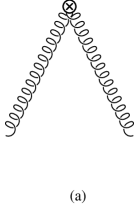
We begin with some terminology. A non-zero momentum insertion means that there is a momentum flowing through the operator vertex. For example, we take $p_{1}$ flowing out one leg, $p_{2}$ flowing in the other, and $Q=p_{1}-p_{2}$ flowing into the vertex as shown in Figure (1a). Gauge independent means that the result is independent of the gauge fixing parameter $\alpha_{r}$. Gauge invariant means that the operator is invariant under the gauge variation defined in Eq. (2.4). A physical matrix element of an operator is an on-shell truncated proper (on-shell amputated one-particle-irreducible) Green function with an insertion of an operator. By on-shell we mean external legs are contracted with physical polarization vectors, put on-mass-shell, and properly renormalized.

We now quote without proof some of the theorems [7], [8], [17] on the renormalization of composite operators in non-Abelian gauge field theories. As has been noted in [7], [8], and [10] these theorems only apply at non-exceptional momentum. That is, the operators should be inserted at non-zero momentum.

Let $G_{i}$ be a set of gauge invariant operators which mix among themselves under renormalization, $A_{i}$ be the set of gauge variant operators which mix with $G_{i}$ under renormalization, and $E_{i}$ be the set of operators which vanish by use of the equations of motion which mix with $G_{i}$ under renormalization.

Theorem 1

$A_{i}$ can be chosen so that it is BRST exact up to equations of motion. i.e.

$$A_{i}\approx\delta_{BRST}B_{i}\,.$$ (20)

Theorem 2

Physical matrix elements of BRST exact operators are zero.

Theorem 3

Physical matrix elements of $E_{i}$ are zero.

Theorem 4

Physical matrix elements of $G_{i}$ are independent of the gauge fixing parameter $\alpha_{r}$.

Theorem 5

The renormalization mixing matrix is triangular. i.e.

$$\left(\begin{array}[]{c}R\left[G\right]\\ R\left[A\right]\\ R\left[E\right]\end{array}\right)=\left(\begin{array}[]{ccc}Z_{GG}&Z_{GA}&Z_{GE}\\ 0&Z_{AA}&Z_{AE}\\ 0&0&Z_{EE}\end{array}\right)\left(\begin{array}[]{c}G\\ A\\ E\end{array}\right).$$ (21)

It is Theorems 2, 4 and 5, that, at first sight, appear to be violated by the work of Hamberg and van Neerven [6] who, following [1] and [3], worked with zero momentum insertions. We demonstrate in the next section that these theorems hold to one loop when one considers non-zero momentum insertions and works in space-time dimension $n>4$.

IV Explicit Calculations

In this section we outline the calculation of the first order physical matrix element with two external gauge fields and an insertion of $O^{GI}_{em}$, $O^{GV}_{em}$, and $O_{g}^{GI}$ at non-zero momentum. We do this in two ways. First, we try a traditional LSZ prescription and a “modified LSZ” prescription [10] and see that these methods fail to respect Theorem 4 given above. Second, we work in $n>4$ space-time dimensions and consider truly massless external legs and find that the theorems given in the previous section are confirmed in our one loop example. As mentioned above, the first order pole pieces of the matrix elements with an insertion of the energy-momentum tensor at non-zero momentum have been studied in detail in [8]. In [10], a detailed study of the energy-momentum tensor inserted at zero momentum was made.

We calculate matrix elements of operators inserted at $Q=p_{1}-p_{2}\neq 0$ thereby introducing another mass scale $Q^{2}$ into the problem. The algebra is therefore more involved than in the case of $Q=0$. The tensor integrals were reduced to scalar integrals as discussed in Appendix B. For this process we performed all algebra on a computer using the program FORM [18], except for the inversion of the large matrices involved, for which we used MAPLE V [19]. The Feynman rules for the vertices containing $O_{em}^{GI}$, $O_{em}^{GV}$, and $O_{g}^{GI}$ are given in Appendix A. We used the gauge field propagator

$$D^{ab}_{\mu\nu}(k)=\frac{\delta^{ab}}{k^{2}}\left(g_{\mu\nu}-(1-\alpha_{r})\frac{k_{\mu}k_{\nu}}{k^{2}}\right)\,,$$ (22)

in all the calculations which follow along with the other standard vertices from the effective Lagrangian.

A Calculating in $n=4$ dimensions

In calculating physical matrix elements when truncating the external propagators one keeps a square root of the residue of the pole of the full propagator for each leg as one goes on-shell. The other square root is discarded with the truncated propagator. To find the residue, note that the full propagator is [20]

$$\widetilde{D}^{ab}_{\mu\nu}(k^{2})=\frac{\delta^{ab}}{k^{2}}\left[\frac{g_{\mu\nu}-k_{\mu}k_{\nu}/k^{2}}{1+\Pi(k^{2})}+\alpha_{r}\frac{k_{\mu}k_{\nu}}{k^{2}}\right].$$ (23)

The self energy of the YM field is well known [21]. It is derived by expanding terms $(-k^{2})^{\epsilon/2}$ for small $\epsilon$, using $x^{\epsilon}=1+\epsilon\ln(x)+\cdots$, then after the contribution from the Lagrangian counterterm is added the $1/\epsilon$ terms cancel and $\epsilon$ is set to zero. However, $k^{2}$ is not set to zero due to the presence of terms in $\ln(-k^{2})$. We write

$$\Pi_{\mu\nu}^{ab}(k)=\delta^{ab}(k_{\mu}k_{\nu}-k^{2}g_{\mu\nu})\Pi(k^{2})\,,$$ (24)

then

$$\Pi(k^{2})=\frac{g_{r}^{2}}{16\pi^{2}}C_{A}\left\{-\frac{31}{9}+\frac{5}{3}\ln(\frac{-k^{2}}{\mu^{2}})+(1-\alpha_{r})\left[1+\frac{1}{2}\ln(\frac{-k^{2}}{\mu^{2}})\right]-\frac{1}{4}(1-\alpha_{r})^{2}\right\}\,,$$ (25)

where we have used the $\overline{MS}$ scheme. The wave function renormalization constant in this scheme is

$$Z_{3}=1-\frac{g_{r}^{2}}{16\pi^{2}}C_{A}\frac{1}{\bar{\epsilon}}\left[\frac{10}{3}+(1-\alpha_{r})\right].$$ (26)

In the above equations ${\bar{\epsilon}}^{-1}=\epsilon^{-1}+\frac{1}{2}\gamma-\frac{1}{2}\ln 4\pi$, $\epsilon=n-4$, $f^{acd}f^{bcd}=\delta^{ab}C_{A}$, $\gamma$ is the Euler constant, and we have extracted the dimension of the coupling by introducing the mass scale $\mu$. We are now in the position to extract the coefficient of the pole as $k^{2}\rightarrow 0$. It is normally chosen as

$$R = \left[1+\Pi(k^{2})|_{k^{2}\rightarrow 0}\right]^{-1}\,,$$ (27)

$$= 1-\frac{g_{r}^{2}}{16\pi^{2}}C_{A}\left\{-\frac{31}{9}+\frac{5}{3}\ln(\frac{-k^{2}}{\mu^{2}})+(1-\alpha_{r})\left[1+\frac{1}{2}\ln(\frac{-k^{2}}{\mu^{2}})\right]-\frac{1}{4}(1-\alpha_{r})^{2}\right\}.$$ (28)

We will see below that if we use

$$\widetilde{R} = \left\{1+\frac{\partial[k^{2}\Pi(k^{2})]}{\partial k^{2}}|_{k^{2}\rightarrow 0}\right\}^{-1}\,,$$ (29)

$$= 1-\frac{g_{r}^{2}}{16\pi^{2}}C_{A}\left\{-\frac{31}{9}+\frac{5}{3}(1+\ln(\frac{-k^{2}}{\mu^{2}}))+(1-\alpha_{r})\left[\frac{3}{2}+\frac{1}{2}\ln(\frac{-k^{2}}{\mu^{2}})\right]-\frac{1}{4}(1-\alpha_{r})^{2}\right\}\,,$$ (30)

as the residue, as suggested by Collins and Scalise [10], then at $Q=0$ the physical matrix element of $O_{em}=O_{em}^{GI}+O_{em}^{GV}$ remains unaffected by higher order corrections and is independent of the gauge fixing parameter $\alpha_{r}$. This absorbs infrared singularities into the asymptotic in and out states much like what one does in proofs of factorization in perturbative QCD.

1 Energy-Momentum Tensor

a Gauge invariant operator, $O_{em}^{GI}$.

FIG. 1.: Diagrams contributing to the physical matrix element of $O_{em}^{GI}$ and $O_{g}^{GI}$ to one loop. A circle with cross denotes an operator insertion.

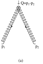
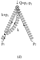
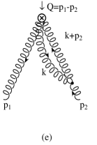
We begin by considering the gauge invariant piece of the energy-momentum tensor. The diagrams relevant for the calculation of the two leg physical matrix element at one loop are shown in Figure 1. The one loop amplitude $A_{\mu\nu}^{ab}(-p_{1},p_{2},2)$ is given by diagrams (b) - (e). Diagram (f), which is constructed using the four leg $O_{em}^{GI}$ vertex is zero in dimensional regularization so it is not considered. We were careful to include the symmetry factor $1/2$ for diagrams (c), (d), and (e) and then partial fraction the resulting expression to remove all terms of the form $k\cdot p_{1}$ and $k\cdot p_{2}$. Next we contracted with polarization vectors and used the on-shell conditions $\epsilon(p_{1})\cdot p_{1}=0=\epsilon(p_{2})\cdot p_{2}$ and $p_{1}^{2}=p_{2}^{2}=m^{2}$ but refrained from setting $m^{2}=0$.

As a check, we set $Q=0$, performed a reduction to scalar integrals, and expanded the resulting expression in powers of $\epsilon=n-4$. The physical matrix element is,

$$<O_{em}^{GI}(0)> = \widetilde{R}Z_{3}\left[T^{ab}_{\mu\nu}(-p,p,2)+A^{ab}_{\mu\nu}(-p,p,2)\right]\epsilon^{\mu}(p)\epsilon^{\nu}(p)\,,$$ (31)

$$= -\delta^{ab}(\Delta\cdot p)^{2}+\delta^{ab}\frac{g_{r}^{2}}{16\pi^{2}}C_{A}(\Delta\cdot p)^{2}\left[3-\frac{3}{2}(1-\alpha_{r})+\frac{1}{4}(1-\alpha_{r})^{2}\right]\,,$$ (32)

where we have used $p_{1}=p_{2}\equiv p$, $\epsilon(p)\cdot p=0$, $p^{2}=0$, and $\epsilon(p)\cdot\epsilon(p)=-1$. If we would have used $R$ instead of $\widetilde{R}$ the coefficients of $\{1,(1-\alpha_{r}),(1-\alpha_{r})^{2}\}$ would have been $\{4/3,-2,1/4\}$. This agrees with [6] and [10] and provides a check on our calculation to this point.

Having made this check we now proceed with the $Q\neq 0$ calculation. The only difference is that the algebra and integrals become more involved. A brief discussion of the methods is found in Appendix B. We quote our findings for the physical matrix element of $O_{em}^{GI}$ as follows:

$$<O_{em}^{GI}(Q)> = \widetilde{R}Z_{3}\left[T^{ab}_{\mu_{1}\mu_{2}}(-p_{1},p_{2},2)+A^{ab}_{\mu_{1}\mu_{2}}(-p_{1},p_{2},2)\right]\epsilon^{\mu_{1}}(p_{1})\epsilon^{\mu_{2}}(p_{2})\,,$$ (33)

$$= \epsilon^{\mu_{1}}(p_{1})\epsilon^{\mu_{2}}(p_{2})T_{\mu_{1}\mu_{2}}^{ab}(-p_{1},p_{2},2)$$ (34)

$$\times \left(1-\frac{g_{r}^{2}}{16\pi^{2}}C_{A}\left\{\frac{11}{2}-\frac{11}{3}\ln\left(\frac{Q^{2}}{m^{2}}\right)+2\ln^{2}\left(\frac{Q^{2}}{m^{2}}\right)\right.\right.$$ (35)

$$+ \left.\left.(1-\alpha_{r})\left[\frac{1}{2}-\ln\left(\frac{Q^{2}}{m^{2}}\right)\right]+\frac{1}{4}(1-\alpha_{r})^{2}\right\}\right)$$ (36)

$$+ \frac{g_{r}^{2}}{16\pi^{2}}C_{A}\left[\epsilon(p_{1})\cdot\epsilon(p_{2})-\frac{p_{1}\cdot\epsilon(p_{2})p_{2}\cdot\epsilon(p_{1})}{p_{1}\cdot p_{2}}\right]$$ (38)

$$\times\left[\frac{2}{3}(\Delta\cdot p_{1})^{2}-(\Delta\cdot p_{1})(\Delta\cdot p_{2})+\frac{2}{3}(\Delta\cdot p_{2})^{2}\right].$$

It is clear that this expression is ill defined at $m^{2}=0$ (so there is a problem with infrared divergences) and is dependent on the gauge fixing parameter $\alpha_{r}$.

b Gauge variant operator, $O_{em}^{GV}$.

FIG. 2.: Diagrams contributing to the physical matrix element of $O_{em}^{GV}$ to one loop. Momenta routings are the same as Figure 1.

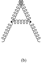
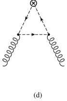
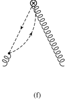
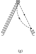
We now consider the gauge variant piece of the energy-momentum tensor. The diagrams relevant for the calculation of the two leg physical matrix element at one loop are shown in Figure 2. The momenta are routed similar to those in Figure 1. The tree level $O_{em}^{GV}$ diagram (a), does not contribute as it vanishes when contracted with polarization vectors. The one loop amplitude $B_{\mu\nu}^{ab}(-p_{1},p_{2})$ is the sum of diagrams (b)-(g) including the symmetry factor $1/2$ for diagram (c). We partial fractioned the resulting expression and used the on-shell conditions as was done for the GI case.

At this point, as a check, we set $Q=0$, performed a reduction to scalar integrals, and expanded the resulting expression in powers of $\epsilon=n-4$. The physical matrix element is,

$$<O_{em}^{GV}(0)> = \widetilde{R}Z_{3}\left[V_{\mu\nu}^{ab}(-p,p)+B_{\mu\nu}^{ab}(-p,p)\right]\epsilon^{\mu}(p)\epsilon^{\nu}(p)\,,$$ (39)

$$= B_{\mu\nu}^{ab}(-p,p)\epsilon^{\mu}(p)\epsilon^{\nu}(p)\,,$$ (40)

$$= -\delta^{ab}\frac{g_{r}^{2}}{16\pi^{2}}C_{A}(\Delta\cdot p)^{2}\left[3-\frac{3}{2}(1-\alpha_{r})+\frac{1}{4}(1-\alpha_{r})^{2}\right]\,,$$ (41)

where we have used $p_{1}=p_{2}\equiv p$, $\epsilon(p)\cdot p=0$, $p^{2}=0$ and $\epsilon(p)\cdot\epsilon(p)=-1$. This again agrees with [10] and gives

$$<O_{em}(0)>=<O_{em}^{GI}(0)>+<O_{em}^{GV}(0)>=-\delta^{ab}(\Delta\cdot p)^{2}.$$ (42)

The form of the physical matrix element of $O_{em}$ is unaffected by higher order corrections and independent of the gauge fixing parameter with the use of $\widetilde{R}$ as the residue instead of $R$.

We now proceed with the $Q$ non-zero result. The only difference is that the algebra and integrals become more involved. For the physical matrix element with $O_{em}^{GV}$ inserted and $Q$ non-zero we find zero. Explicitly,

$$<O_{em}^{GV}(Q)> = \widetilde{R}Z_{3}\left[V_{\mu_{1}\mu_{2}}^{ab}(-p_{1},p_{2})+B_{\mu_{1}\mu_{2}}^{ab}(-p_{1},p_{2})\right]\epsilon^{\mu_{1}}(p_{1})\epsilon^{\mu_{2}}(p_{2})\,,$$ (43)

$$= B_{\mu_{1}\mu_{2}}^{ab}(-p_{1},p_{2})\epsilon^{\mu_{1}}(p_{1})\epsilon^{\mu_{2}}(p_{2})\,,$$ (44)

$$= 0.$$ (45)

Which is in agreement with the Theorem 2 and is not affected by what we choose for $R$ because the tree level diagram $V_{\mu_{1}\mu_{2}}^{ab}(-p_{1},p_{2})$ vanishes when contracted with polarization vectors satisfying $\epsilon(p)\cdot p=0$.

By looking at Eq. (31) we see that Theorem 4 is violated so at this point we already notice a problem. By looking at Eq. (39) we see that Theorem 2 is also violated. However, Eq. (43) confirms Theorem 2 but Eq. (33) has IR divergences in the form $\ln^{i}(Q^{2}/m^{2}),i=1,2$ that must be removed. They are due to the order of our limits, namely, we took the limit $\epsilon\rightarrow 0$ too soon.

Since there is an IR divergence we can extract it by reworking the calculation and taking the limits $p_{1}^{2}\rightarrow 0$ and $p_{2}^{2}\rightarrow 0$ before $\epsilon\rightarrow 0$. In dimensional regularization, with space-time dimension $n=4+\epsilon$, both the UV and IR divergences are regulated. After UV renormalization, which is performed at $\epsilon<0$ we can analytically continue to $\epsilon>0$ which regulates the IR singularities. This allows us to set the square of the momenta of the external gluon lines to zero because $(p_{1}^{2})^{\epsilon/2}=0=(p_{2}^{2})^{\epsilon/2}$ so long as $\epsilon>0$. This interchange of the order of the limits is the crux of our new calculation which we present next.

B Calculating in $n>4$ dimensions

In contrast to the previous section, here we reverse the order of limits and find that Theorem 4 is now satisfied. That is, we consider $\epsilon>0$ so that $(-k^{2})^{\epsilon/2}=0$ in the limit $k^{2}=0$. This implies that the residue factors $RZ_{3}$ of the previous section are to be set to unity. We will see that doing this leads to a universal double and single pole structure that allows use to determine the anomalous dimension of the gluon operator.

1 Energy-momentum tensor revisited

a Gauge invariant operator, $O_{em}^{GI}$.

We now return to the gauge invariant piece of the energy-momentum tensor. The diagrams relevant for the calculation of the two particle physical matrix element at one loop are shown in Figure 1. Diagram (f), which is constructed using the four leg $O_{em}^{GI}$ vertex, is zero in dimensional regularization. Also, because we set $(p_{1}^{2})^{\epsilon/2}=0=(p_{2}^{2})^{\epsilon/2}$ diagrams (d) and (e) vanish. We partial fractioned the expression resulting from diagrams (b) and (c) to remove all terms of the form $k\cdot p_{1}$ and $k\cdot p_{2}$. Next we contracted with polarization vectors $\epsilon^{\mu_{1}}(p_{1})$ and $\epsilon^{\mu_{2}}(p_{2})$ and used the on-shell conditions $\epsilon(p_{1})\cdot p_{1}=0=\epsilon(p_{2})\cdot p_{2}$ and $p_{1}^{2}=0=p_{2}^{2}$ remembering that $(p_{1}^{2})^{\epsilon/2}=0=(p_{2}^{2})^{\epsilon/2}$ as $\epsilon>0$. A discussion of the methods for evaluating the resulting integrals is found in Appendix B. Adding diagram (a) we quote our findings for the sum of all the diagrams in Figure 1 with $O_{em}^{GI}$ inserted at $Q$ and external legs on-shell as defined above as follows:

$$<O_{em}^{GI}(Q)> = 1\left[T^{ab}_{\mu_{1}\mu_{2}}(-p_{1},p_{2},2)+A^{ab}_{\mu_{1}\mu_{2}}(-p_{1},p_{2},2)\right]\epsilon^{\mu_{1}}(p_{1})\epsilon^{\mu_{2}}(p_{2})\,,$$ (46)

$$= \epsilon^{\mu_{1}}(p_{1})\epsilon^{\mu_{2}}(p_{2})T_{\mu_{1}\mu_{2}}^{ab}(-p_{1},p_{2},2)$$ (47)

$$\times \left\{1+g_{r}^{2}C_{A}S_{n}(-\frac{Q^{2}}{\mu^{2}})^{\epsilon}\left[-\frac{8}{\epsilon^{2}}+\frac{-4\gamma_{E}+22/3}{\epsilon}+h(2)\right]\right\}$$ (48)

$$+ g_{r}^{2}C_{A}S_{n}(-\frac{Q^{2}}{\mu^{2}})^{\epsilon}\left[\epsilon(p_{1})\cdot\epsilon(p_{2})-\frac{p_{1}\cdot\epsilon(p_{2})p_{2}\cdot\epsilon(p_{1})}{p_{1}\cdot p_{2}}\right]$$ (50)

$$\times\left[\frac{2}{3}(\Delta\cdot p_{1})^{2}-(\Delta\cdot p_{1})(\Delta\cdot p_{2})+\frac{2}{3}(\Delta\cdot p_{2})^{2}\right]\,,$$

where $C_{A}=N_{c}=3$, $S_{n}=\pi^{n/2}/(2\pi)^{n}$, and $T^{ab}_{\mu_{1}\mu_{2}}(-p_{1},p_{2},2)$ is the Born level vertex for the classical energy-momentum tensor given explicitly in Appendix A. The factor of $\mu^{-2\epsilon}$ is the dimension of the coupling $g_{r}$. The finite term $h(2)$ is given later in Eq. (59) for completeness.

At this point we pause to note several important things. One, this result is independent of the gauge fixing parameter in agreement with Theorem 4. Two, because we are considering on-shell legs we have not multiplied by an LSZ type residue when truncating the legs. Three, there are both double and single Sudakov IR poles. Four, there is a new finite form factor that was not present at the Born level. Five, if we take the limit $Q^{2}\rightarrow 0$ for $\epsilon>0$ the only piece that survives is the Born level vertex. We will return to these points in the discussion below.

b Gauge variant operator, $O_{em}^{GV}$.

We now return to the gauge variant piece of the energy-momentum tensor. The diagrams relevant for the calculation of the corresponding physical matrix element with an insertion of $O_{em}^{GV}$ at one loop order are shown in Figure 2. The momenta are routed similar to those in Figure 1. Again, (f) and (g) vanish. The tree level $O_{em}^{GV}$ diagram (a), does not contribute as it vanishes on-shell. After performing the integrations as above the result vanishes, which is in agreement with the Theorem 2. Explicitly,

$$<O_{em}^{GV}(Q)> = 1\left[V_{\mu_{1}\mu_{2}}^{ab}(-p_{1},p_{2})+B_{\mu_{1}\mu_{1}}^{ab}(-p_{1},p_{2})\right]\epsilon^{\mu_{1}}(p_{1})\epsilon^{\mu_{2}}(p_{2})\,,$$ (51)

$$= B_{\mu_{1}\mu_{2}}^{ab}(-p_{1},p_{2})\epsilon^{\mu_{1}}(p_{1})\epsilon^{\mu_{2}}(p_{2})\,,$$ (52)

$$= 0.$$ (53)

2 Gluon operator

Now consider the twist two gauge invariant gluon operator. The one loop diagrams are shown in Figure 1. We followed the same procedure as outlined above for the revisited energy-momentum tensor but this time we took the liberty of setting $\Delta\cdot p_{1}=\Delta\cdot p_{2}\equiv\Delta\cdot p$ which allows us to do the integration by parts described at the end of Section II. The necessary integrals are discussed in Appendix B. We quote the result for the sum of all diagrams on-shell as defined above:

$$<O_{g}^{GI}(Q)> = 1\left[T^{ab}_{\mu_{1}\mu_{2}}(-p_{1},p_{2},m)+A^{ab}_{\mu_{1}\mu_{2}}(-p_{1},p_{2},m)\right]\epsilon^{\mu_{1}}(p_{1})\epsilon^{\mu_{2}}(p_{2})\,,$$ (54)

$$= \epsilon^{\mu_{1}}(p_{1})\epsilon^{\mu_{2}}(p_{2})T_{\mu_{1}\mu_{2}}^{ab}(-p_{1},p_{2},m)$$ (55)

$$\times \left\{1+g_{r}^{2}C_{A}S_{n}(-\frac{Q^{2}}{\mu^{2}})^{\epsilon}\left[-\frac{8}{\epsilon^{2}}+\frac{-4\gamma_{E}+22/3+\gamma^{(m)}_{gg}/C_{A}}{\epsilon}+h(m)\right]\right\}$$ (56)

$$+ g_{r}^{2}C_{A}S_{n}(-\frac{Q^{2}}{\mu^{2}})^{\epsilon}(\Delta\cdot p)^{m}f(m)\left[\epsilon(p_{1})\cdot\epsilon(p_{2})-\frac{p_{1}\cdot\epsilon(p_{2})p_{2}\cdot\epsilon(p_{1})}{p_{1}\cdot p_{2}}\right]\,,$$ (57)

where $T_{\mu_{1}\mu_{2}}^{ab}(-p_{1},p_{2},m)$ is the Born level vertex for the gauge invariant gluon operator given in Appendix A. All other symbols are as defined below Eq. (46) and $\gamma^{(m)}_{gg}$ is the one loop anomalous dimension of the gluon operator [1]

$$\gamma^{(m)}_{gg}=C_{A}\left(\frac{8}{m+2}-\frac{8}{m+1}+\frac{16}{m}-\frac{8}{m-1}+8\sum_{i=1}^{m-1}\frac{1}{i}-\frac{22}{3}\right).$$ (58)

The finite functions $h(m)$ and $f(m)$ are given by

$$h(m) = -\gamma_{E}^{2}+\frac{\gamma_{E}}{2}\left(\frac{\gamma_{gg}^{(m)}}{C_{A}}+\frac{22}{3}\right)+\frac{\pi^{2}}{6}$$ (59)

$$- 8\widetilde{S}(m-2)-8S_{1}(m-1)\left(\frac{1}{m+2}-\frac{1}{m+1}+\frac{2}{m}\right)$$ (60)

$$- \frac{8}{(m+2)^{2}}+\frac{12}{m+2}+\frac{8}{(m+1)^{2}}-\frac{16}{m+1}-\frac{16}{m^{2}}+\frac{4}{m}\,,$$ (61)

and

$$f(m)=4\left(\frac{-1}{m+2}+\frac{1}{m+1}\right)\,,$$ (62)

where

$$S_{i}(n)=\sum_{l=1}^{n}\frac{1}{l^{i}}\,,$$ (63)

$$\widetilde{S}(n)=\sum_{l=1}^{n}\left(\begin{array}[]{c}n\\ l\end{array}\right)\frac{(-1)^{l+1}}{l^{2}}=\frac{1}{2}S_{2}(n-1)+\frac{1}{n}S_{1}(n)+\frac{1}{2}S_{1}^{2}(n-1)\,.$$ (64)

The same points we noted below Eq. (46) apply here and are discussed below. In addition, we note that the coefficient of the double pole is the same as that in Eq. (46), i.e. it is universal, and that the coefficient of the single pole contains the anomalous dimension of the gluon operator in addition to the terms in Eq. (46).

V Discussion and Conclusions

We now return to the three points of contention listed in the introduction. There are two reasons why the matrix elements of the GV operators used by Hamberg and van Neerven [6] did not vanish. One is that their operators are not BRST exact. Therefore, Theorem 2 does not apply. One can see this by simply checking that at Born level their $O_{a}$ does not vanish on-shell when $Q\neq 0$. Even if they had used an operator that was BRST exact they would have found it had a non-vanishing physical matrix element because Theorem 2 breaks down when the operator is inserted at zero momentum as was shown in detail by Collins and Scalise [10]. The fact that Theorem 2 breaks down at one loop for a zero momentum insertion means that at two loops one will see a non-triangular mixing matrix, hence the apparent demise of Theorem 5. By inserting BRST exact operators at non-zero momentum we have shown Theorem 2 works at one loop and we therefore have no reason to doubt Theorem 5.

The gauge parameter dependence of the physical matrix element of the gauge invariant gluon operator was not investigated by the first group attempting a two loop calculation in the covariant gauge [3]. They worked in the Feynman gauge. Hamberg and van Neerven noticed this gauge dependence as they calculated the $O(\alpha_{s})$ terms in the general covariant gauge. They claimed that this implied a renormalization of the gauge parameter in the two loop calculation to keep the coefficients of the single pole terms gauge independent. They then proceeded with the two loop calculation in the Feynman gauge. Hence, they can not make a statement on the gauge parameter dependence of the finite terms at two loops. A finite gauge parameter dependence at two loops can lead to $1/\epsilon$ gauge parameter dependence at three loops. This would imply a gauge dependent anomalous dimension. As we demonstrated, our result is independent of the gauge fixing parameter at one loop. It is now safe to proceed to two loops.

In our method we put the momentum squared of the external legs to zero at the very beginning. This is possible because we work in $n>4$ dimensions and only after extracting the IR safe anomalous dimension do we let $n\rightarrow 4$. Because we worked with physical legs the LSZ residue is unity. We also notice a double and single Sudakov pole structure arising because we set the momentum squared of the external legs to zero in the very beginning. We conjecture that these factors are universal to all three point functions involving two external gluon legs. An all orders proof of the universality may be possible and a two loop calculation of the energy-momentum tensor is technically possible and would serve as a check on these ideas. A detailed study of the universality of double and single pole structure will also yield information on the finite form factor seen in Eq. (46) and Eq. (54). As can be seen from Eq. (46) it is safe to let $Q^{2}\rightarrow 0$ as $\epsilon>0$ (only IR divergences remain) leaving only the Born level result. The same is true for Eq. (54) after the UV counter term has been added.

The fact that it took so long to verify the general theorems was anticipated in [8] where, following the proofs of the general theorems, there are statements like

…matrix elements of $\tilde{N}(x)$ vanish if the on-shell limit can be taken. …but for pure Yang-Mills theory, the on-shell limit cannot be taken because of infrared divergences …

It is only by seeing that these infrared divergences are universal if regulated dimensionally that we are able to overcome these problems and verify the general theorems. Our method of calculation has actually been applied to the two loop anomalous dimension of the nonsinglet quark operator [22] where the complications of GI and GV operator mixing do not enter and where the $\alpha_{s}C_{F}$ and $\alpha_{s}^{2}n_{f}C_{F}$ terms were found to be in agreement with the Sudakov factorization theorems [11].

To conclude, we have presented new one loop calculations that vindicate the general theorems of Joglekar and Lee which were recently called into question by the work of Hamberg and van Neerven. In the process we have found a new method of calculating the anomalous dimension of the gluon operator. We did this by considering physical matrix elements with insertions of the appropriate operator at non-zero momentum with the resulting IR singularities being regulated dimensionally. We found that the physical matrix element of either the classical energy-momentum tensor or the gauge invariant gluon operator is independent of the gauge fixing parameter. We also found that a physical matrix element of the BRST exact gauge variant operator that enters the full energy-momentum tensor vanishes. A universal Sudakov factor appears in both the physical matrix elements of the energy-momentum tensor and of the gluon operator. The universality of this factor and the UV finiteness of the energy-momentum tensor then provide another method for determining the gluon anomalous dimension which we conjecture applies to higher loops as well.

Acknowledgements

The authors thank John Collins and Randy Scalise for many stimulating discussions. We also acknowledge George Sterman for a helpful discussion and Willy van Neerven and Peter van Nieuwenhuizen for comments. The work in this paper was supported in part by the contract NSF 9309888.

A Feynman Rules

FIG. 3.: Feynman rules for $O_{em}^{GI}$ and $O_{g}^{GI}$

FIG. 4.: Feynman rules for $O_{em}^{GV}$

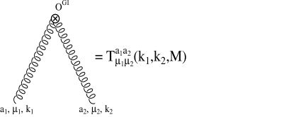
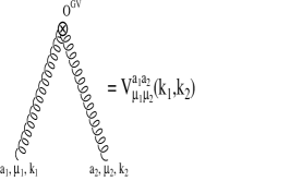
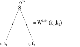
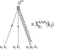
The operators $O_{em}^{GI}$, $O_{g}^{GI}$ and $O_{em}^{GV}$ have the following Feynman rules as shown in Figures 3 and 4. All momenta flow into the vertices.

$$T_{\mu_{1}\mu_{2}}^{a_{1}a_{2}}(k_{1},k_{2},M) = -\frac{1}{2}\delta^{a_{1}a_{2}}\left[(\Delta\cdot k_{1})^{M-2}+(\Delta\cdot k_{2})^{M-2}\right]$$ (A1)

$$\times \left[\Delta_{\mu_{1}}\Delta_{\mu_{2}}\,k_{1}\!\cdot\!k_{2}-\Delta_{\mu_{1}}k_{1\mu_{2}}\,\Delta\!\cdot\!k_{2}\right.$$ (A2)

$$- \left.\Delta_{\mu_{2}}k_{2\mu_{1}}\,\Delta\!\cdot\!k_{1}+\Delta\!\cdot\!k_{1}\,\Delta\!\cdot\!k_{2}\,g_{\mu_{1}\mu_{2}}\right]\,,$$ (A3)

$$U_{\mu_{1}\mu_{2}\mu_{3}}^{a_{1}a_{2}a_{3}}(k_{1},k_{2},k_{3}) = -igf^{a_{1}a_{2}a_{3}}$$ (A4)

$$\times \left[\Delta_{\mu_{1}}(k_{1\mu_{2}}\Delta_{\mu_{3}}-\Delta_{\mu_{2}}k_{1\mu_{3}})+\Delta\!\cdot\!k_{1}(g_{\mu_{1}\mu_{3}}\Delta_{\mu_{2}}-g_{\mu_{1}\mu_{2}}\Delta_{\mu_{3}})\right.$$ (A5)

$$+ \left.\Delta_{\mu_{2}}(k_{2\mu_{3}}\Delta_{\mu_{1}}-\Delta_{\mu_{3}}k_{2\mu_{1}})+\Delta\!\cdot\!k_{2}(g_{\mu_{2}\mu_{1}}\Delta_{\mu_{3}}-g_{\mu_{2}\mu_{3}}\Delta_{\mu_{1}})\right.$$ (A6)

$$+ \left.\Delta_{\mu_{3}}(k_{3\mu_{1}}\Delta_{\mu_{2}}-\Delta_{\mu_{1}}k_{3\mu_{2}})+\Delta\!\cdot\!k_{3}(g_{\mu_{3}\mu_{2}}\Delta_{\mu_{1}}-g_{\mu_{3}\mu_{1}}\Delta_{\mu_{2}})\right]\,,$$ (A7)

$$V_{\mu_{1}\mu_{2}}^{a_{1}a_{2}}(k_{1},k_{2}) = \frac{1}{\alpha}\delta^{a_{1}a_{2}}\left[k_{1}^{\mu_{1}}\Delta^{\mu_{2}}\Delta\cdot k_{1}+k_{2}^{\mu_{2}}\Delta^{\mu_{1}}\Delta\cdot k_{2}\right]\,,$$ (A8)

$$W^{a_{1}a_{2}}(k_{1},k_{2}) = \delta^{a_{1}a_{2}}\,\Delta\!\cdot\!k_{1}\,\Delta\!\cdot\!k_{2}\,,$$ (A9)

$$X^{a_{1}a_{2}a_{3}}_{\mu_{3}}(k_{3}) = -igf^{a_{1}a_{2}a_{3}}\,\Delta\!\cdot\!k_{1}\,\Delta_{\mu_{3}}\,.$$ (A10)

$T_{\mu_{1}\mu_{2}}^{a_{1}a_{2}}(k_{1},k_{2},M=2)$ is the Born level energy-momentum operator vertex and $V_{\mu_{1}\mu_{2}}^{a_{1}a_{2}}(k_{1},k_{2})$ vanishes when contracted with polarization vectors satisfying $\epsilon(k)\cdot k=0$.

B Integrals

In this appendix we briefly discuss some technicalities of the calculation. For the case of $Q=0$ all integrals are expressible in terms of Eq. (B2) below. The case of $Q\neq 0$ is more complicated and we discuss it now. After partial fractioning the amplitudes we find everything is expressible in terms of the integrals

$$J(a,b,c,M)_{\{\;,\mu,\mu\nu\}}=\int\frac{d^{n}k}{(2\pi)^{n}}\frac{\{1,k_{\mu},k_{\mu}k_{\nu}\}(\Delta\cdot k)^{M}}{(k^{2})^{a}[(k+p_{1})^{2}]^{b}[(k+p_{2})^{2}]^{c}}\,.$$ (B1)

We write these integrals as linearly independent tensor structures multiplied by undetermined coefficients. We then contract both sides with the various independent tensor structures and get a set of linear equations. These we invert and solve for the previously undetermined coefficients. At this point we have expressions for the tensor integrals above in terms of the scalar integral $J(a,b,c,M)$ and the tensor integrals with only two denominators, namely

$$I(a,b,M)_{\{\;,\mu,\mu\nu\}}=\int\frac{d^{n}k}{(2\pi)^{n}}\frac{\{1,k_{\mu},k_{\mu}k_{\nu}\}(\Delta\cdot k)^{M}}{(k^{2})^{a}[(k+p)^{2}]^{b}}\,,$$ (B2)

which we again decompose as above. The remaining integrals are expressible in terms of

$$I(a,b,M) = iS_{n}(-1)^{n/2}(p^{2})^{n/2-a-b}(-1)^{M}(\Delta\cdot p)^{M}$$ (B3)

$$\times \frac{\Gamma(a+b-n/2)}{\Gamma(a)\Gamma(b)}\frac{\Gamma(n/2-a+M)\Gamma(n/2-b)}{\Gamma(n+M-a-b)}\,,$$ (B4)

and, for the $p_{1}^{2}=p_{2}^{2}=m^{2}$ case, the specific cases $J(1,1,1,0)$, $J(1,1,2,0)=J(1,2,1,0)$, $J(2,2,1,0)=J(2,1,2,0)$ and $J(2,1,1,0)$. In the above formulae $S_{n}=\pi^{n/2}/(2\pi)^{n}$. The scalar $J$ integrals listed above can be found in the literature [23]. We list the cases of interest here for completeness. The integral $J(1,1,1,0)$ is finite in four dimensions for $m^{2}\neq 0$:

$$J(1,1,1,0)=\frac{i}{16\pi^{2}}\frac{1}{Q^{2}}x\Phi(x)$$ (B5)

where

$$\Phi(x) = \frac{1}{\lambda(x)}\left\{2\ln\left[\frac{x-\lambda(x)}{2}\right]\ln\left[\frac{2-x-\lambda(x)}{2}\right]\right.$$ (B6)

$$- \left.2{\rm Li_{2}}\left[\frac{x-\lambda(x)}{2}\right]-2{\rm Li_{2}}\left[\frac{2-x-\lambda(x)}{2}\right]+\frac{\pi^{2}}{3}\right\}$$ (B7)

where ${\rm Li_{2}}$ is the dilogarithm function and

$$\lambda(x) = x\sqrt{1-4/x}$$ (B8)

$$x = Q^{2}/m^{2}.$$ (B9)

From the above and properties of the dilogarithm function one can work out that

$$Re[x\Phi(x)]\rightarrow\left\{\begin{array}[]{ccc}\ln^{2}(x)&as&x\rightarrow\infty\\ \ln^{2}(-x)&as&x\rightarrow-\infty\end{array}\right\}$$ (B10)

The other $J$ integrals have poles in $n-4$. They are, dropping terms $O(n-4)$,

$$J(2,1,1,0) = iS_{n}\left[\frac{2}{n-4}-\ln\left(\frac{-Q^{2}}{\mu^{2}}\right)+2\ln\left(\frac{-m^{2}}{\mu^{2}}\right)+\gamma\right]\frac{1}{m^{4}}$$ (B11)

$$J(1,2,1,0) = iS_{n}\left[\frac{2}{n-4}+\ln\left(\frac{-Q^{2}}{\mu^{2}}\right)+\gamma\right]\frac{1}{Q^{2}m^{2}}$$ (B12)

$$J(2,1,2,0) = iS_{n}\left[\frac{2}{n-4}(Q^{2}+m^{2})-Q^{2}+2Q^{2}\ln\left(\frac{-m^{2}}{\mu^{2}}\right)\right.$$ (B13)

$$+ \left.(m^{2}-Q^{2})\ln\left(\frac{-Q^{2}}{\mu^{2}}\right)+\gamma\right]\frac{1}{Q^{2}m^{6}}$$ (B14)

where $p_{1}^{2}=p_{2}^{2}=m^{2}$, $Q=p_{1}-p_{2}$, $\gamma$ is the Euler constant and the renormalization scale, which comes from the coupling constant implied on both sides of the formulae, is chosen to be $\mu^{2}$. Note that the terms in $\ln(\mu^{2})$ cancel in the final answers given in Section IV.

Whereas for the $p_{1}^{2}=0=p_{2}^{2}$ case we need

$$J(a,b,c,M) = i(-1)^{n/2}S_{n}(Q^{2})^{n/2-a-b-c}(-\Delta\cdot p_{2})^{M}$$ (B17)

$$\times\frac{\Gamma(a+b+c-n/2)\Gamma(n/2-a-c)}{\Gamma(b)\Gamma(c)}\frac{\Gamma(n/2+M-a-b)}{\Gamma(n+M-a-b-c)}$$

$$\times F_{2,1}\left(-M,\frac{n}{2}-a-c;1-\frac{n}{2}-M+a+b;\frac{\Delta\cdot p_{1}}{\Delta\cdot p_{2}}\right)\,,$$

where $Q^{2}=-2p_{1}\cdot p_{2}\neq 0$, and $F_{2,1}(\alpha,\beta;\gamma;z)$ is the hypergeometric function of one variable. Both scalar integrals Eq. (B3) and Eq. (B17) can be derived by repeated differentiation of the $M=0$ integral or by the method of [24]. We have checked that both methods agree with each other and, for $M=2,4$ and 6, with the standard Passarino-Veltman reduction techniques [25]. As stated in Section II, we use the condition $\Delta\cdot p_{1}=\Delta\cdot p_{2}$. Thus, the hypergeometric function in Eq. (B17) reduces to products of Gamma functions.

REFERENCES

- [1] D. J. Gross and F. Wilczek, Phys. Rev. D 9, 980 (1974); H. Georgi and H. D. Politzer, Phys. Rev. D 9, 416 (1974).
- [2] W. Furmanski and R. Petronzio, Phys. Lett. B 97, 437 (1980).
- [3] E. G. Floratos, D. A. Ross and C. T. Sachrajda, Nucl. Phys. B152, 493 (1979); A. Gonzalez-Arroyo and C. Lopez, ibid. B166, 429 (1980); E. G. Floratos, C. Kounnas and R. Lacaze, Phys. Lett. B 98, 285 (1981).
- [4] I. Antoniadis and E. G. Floratos, Nucl. Phys. B191, 217 (1981).
- [5] E. B. Zijlstra and W. L. van Neerven, Nucl. Phys. B383, 525 (1992).
- [6] R. Hamberg and W.L. van Neerven, Nucl. Phys. B379, 143 (1992); R. Hamberg, Ph.D. thesis, University of Leiden, 1991.
- [7] S. D. Joglekar and B. W. Lee, Ann. Phys. (N.Y.) 97, 160 (1976); S. Joglekar, ibid. 100, 395 (1976); 108, 233 (1977); 109, 210 (1977).
- [8] C. Lee, Phys. Rev. D 14, 1078 (1976).
- [9] J. A. Dixon and J. C. Taylor, Nucl. Phys. 78, 552 (1974).
- [10] J. C. Collins and R. J. Scalise, PSU/TH/141, to appear in Phys. Rev. D.
- [11] J. C. Collins, in Perturbative Quantum Chromodynamics edited by A.H. Mueller (World Scientific, New Jersey, 1989).
- [12] C. Becchi, A. Rouet, and R. Stora, Commun. Math. Phys. 42, 127 (1975); Ann. Phys. (N.Y.) 98, 287 (1976).
- [13] I. V. Tyutin, Gauge Invariance in Field Theory and Statistical Physics in Operator Formalism, LEBEDEV-75-39 (unpublished).
- [14] D. Freedman, I. Muzinich, and E. Weinberg, Ann. Phys. (N.Y.) 87, 95 (1974).
- [15] L. D. Landau and E. M. Lifshitz, The Classical Theory of Fields, 4th Edition (Pergamon Press, Oxford, 1975) Section 94.
- [16] M. Henneaux, Phys. Lett. B 313, 35 (1993); erratum 316, 633 (1993).
- [17] J. C. Collins, Renormalization (Cambridge University Press, New York, 1984).
- [18] J. A. M. Vermaseren, FORM Version 2.2b, CAN, Amsterdam, The Netherlands, 1991.
- [19] Symbolic Computation Group, MAPLE V, University of Waterloo, Ontario, Canada, 1991.
- [20] T. Muta, Foundations of Quantum Chromodynamics: An Introduction to Perturbative Methods in Gauge Theories (World Scientific, New Jersey, 1987), p. 170.
- [21] W. Celmaster and R. Gonsalves, Phys. Rev. D 20, 1420 (1979).
- [22] T. Matsuura, Internal Report (Doctoraal Scriptie), University of Leiden, 1986.
- [23] A. I. Davydychev, J. Phys. A 25, 5587 (1992).
- [24] A. I. Davydychev, Phys. Lett. B 263, 107 (1991).
- [25] G. Passarino and M. Veltman, Nucl. Phys. B160, 151 (1979); W.J.P. Beenakker, Ph.D. Thesis, University of Leiden, 1989.