CERN-TH.7449/94

The $1/m_{Q}$ Expansion in QCD:
Introduction and Overview

Thomas Mannel

Theory Division, CERN, CH-1211 Geneva 23, Switzerland

A mini-review of the heavy mass expansion in QCD is given. We focus on exclusive semileptonic decays and some topics of recent interest in inclusive decays of heavy hadrons.

Contribution to the Workshop QCD 94, Montpellier, 7-13 July 1994

CERN-TH.7449/94
September 1994

1 Introduction

In the past five years considerable progress has been made towards a QCD-based and model independent description of hadrons containing a heavy-flavour quark. This progress has been achieved by the use of the heavy mass limit for the heavy quark, in which it is replaced by a static source of a colour field. This limit of QCD leads to a well-defined field theory, the so-called Heavy Quark Effective Theory (HQET).

The infinite mass limit from QCD has been used for some time for various purposes [1], but the main observation, which triggered the enormous development of this field, is that in the infinite mass limit two additional symmetries appear, which are not present in full QCD [2]. Since then the implications of the heavy mass limit and HQET have been extensively studied in innumerable publications, and the development of the field is documented in more or less extensive reviews [3].

The two additional symmetries of the heavy mass limit have important phenomenological applications; they lead to model-independent relations between form factors describing e.g. exclusive weak decays. The origin of the new symmetries is quite simple. The first symmetry is a heavy-flavour symmetry, which is due to the fact that the interaction of the quarks with the gluons is flavour-blind and in the heavy mass limit all heavy quarks act as a static source of colour. Formally this corresponds to an $SU(2)$ symmetry relating $b$ and $c$ quarks moving with the same velocity. The second symmetry is the spin symmetry of the heavy quark. The interaction of the heavy quark spin with the “chromomagnetic” field is inversely proportional to the heavy mass and hence vanishes in the infinite mass limit. As a consequence, the rotations for the heavy quark spin become an $SU(2)$ symmetry, which holds for a fixed velocity of the heavy quark.

Corrections to the limit $m_{Q}\to\infty$ may be studied systematically in the framework of HQET. The corrections are given as power series expansions in two small parameters. The first small parameter is the strong coupling constant, taken at the scale of the heavy quark $\alpha_{s}(m_{Q})$. This type of correction may be calculated systematically using perturbation theory in HQET. The second type of correction is characterized by the small parameter $\bar{\Lambda}/m_{Q}$, where $\bar{\Lambda}$ is a scale of the light QCD degrees of freedom, e.g. $\bar{\Lambda}\sim m_{hadron}-m_{Q}$. In the effective theory approach this type of corrections enter through operators of higher dimension, the matrix elements of which have to be parametrized in general by additional form factors.

More or less parallel to the development of heavy quark symmetry and HQET, which is well suited for exclusive decays, the heavy mass expansion has been applied also to inclusive decays [4]-[10]. The heavy quark mass sets a scale that is large compared to $\Lambda_{QCD}$, and one may use a similar setup as in deep inelastic scattering for the inclusive decays; in particular, the operator product expansion for the inclusive decays yields an expansion in inverse powers of the heavy quark mass. In this way one may not only study total rates, but also differential distributions such as the lepton energy spectra in inclusive semileptonic decays.

This mini-review is intended to set up the stage for some of the contributions to this conference, which present in some detail new calculations in HQET or new results for inclusive heavy hadron decays. It is divided into two parts, one dealing with HQET and exclusive decays and the second devoted to inclusive decays.

In the next section we discuss the heavy mass limit of QCD and the additional symmetries of this limit. We formulate HQET, including terms up to order $1/m^{2}$. The strategy of a HQET calculation is outlined and applied to the weak decay matrix elements relevant for the semileptonic decays $B\to D^{(*)}\ell\nu$. In section 3 we consider the setup for the heavy mass expansion for inclusive decays and study the rate and differential distributions in inclusive semileptonic decays. Finally we comment on inclusive non-leptonic processes and inclusive rare decays and conclude.

2 Heavy Quark Effective Theory

The Green functions of QCD containing a heavy quark in general depend on its mass $m_{Q}$. This mass sets a scale that is large compared to the scale $\bar{\Lambda}$, which characterizes the light degrees of freedom, $\bar{\Lambda}/m_{Q}$ is small and becomes a reasonable expansion parameter. The leading order in this parameter corresponds to the infinite mass limit of QCD, which corresponds to an effective theory where the degrees of freedom related to this large scale have been removed. This effective theory, the so-called HQET, may be formulated as a Lagrangian field theory, and its Lagrangian may be obtained from QCD. There are several ways to construct this Lagrangian and the one closest to the idea of “integrating out” heavy degrees of freedom is discussed in [11], where the small components of the heavy quark spinor field are identified as the heavy degrees of freedom and are removed by integrating over them in the generating functional of QCD Green functions.

We shall not go through any derivation here, but rather state the result and its relation to full QCD. We denote the heavy quark field of full QCD by $Q$ and define

$$Q_{v}(x)=\exp(im_{Q}vx)Q(x)=h_{v}(x)+H_{v}(x),$$ (1)

where $v$ is a velocity ($v^{2}=1$), which is later identified with the velocity of the heavy hadron. Extracting this phase factor from the full QCD field $Q$ removes the dominant part $m_{Q}v$ of the heavy quark momentum, since this phase redefinition corresponds to a splitting of the heavy quark momentum according to $p=m_{Q}v+k$, where the residual momentum $k$ is small, of the order of $\bar{\Lambda}$. Furthermore, $h_{v}$ ($H_{v}$) is the large (small) component field, corresponding to the projections

$$h_{v}=P_{+}Q_{v},\quad H_{v}=P_{-}Q_{v},\quad P_{\pm}=\frac{1}{2}(1\pm v\hskip-5.0pt/).$$ (2)

The small component field $H_{v}$ is related to the large scale $m_{Q}$; integrating out $H_{v}$ from the generating functional of QCD Green functions corresponds to the replacement

$$H_{v}=P_{-}\left(\frac{1}{2m+ivD}\right)iD\hskip-5.0pt/h_{v}$$ (3)

and this yields a non-local “Lagrangian” of the form [11]

$${\cal L}=\bar{h}_{v}(ivD)h_{v}+\bar{h}_{v}iD\hskip-5.0pt/P_{-}\left(\frac{1}{2m+ivD}\right)iD\hskip-5.0pt/h_{v},$$ (4)

which still contains all orders in $1/m_{Q}$. However, the non-locality appearing in the second term of (4) may be expanded into an infinite series of local terms, which come with increasing powers of $1/m_{Q}$. Hence one may in this way establish the desired heavy mass expansion for the Lagrangian. The first few terms of this expansion are

$${\cal L}=\bar{h}_{v}(ivD)h_{v}+\left(\frac{1}{2m}\right)\bar{h}_{v}iD\hskip-5.0pt/P_{-}iD\hskip-5.0pt/h_{v}+\left(\frac{1}{2m}\right)^{2}\bar{h}_{v}iD\hskip-5.0pt/P_{-}(-ivD)iD\hskip-5.0pt/h_{v}+\cdots$$ (5)

The non-local expression (4) is still equivalent to full QCD; in particular it is independent of the still arbitrary velocity vector $v$. In fact, the Lagrangian (4) is invariant under an infinitesimal shift of the velocity

$$v\to v+\delta v\qquad v\cdot\delta v=0$$ (6)

$$h_{v}\to h_{v}+\frac{\delta v\hskip-7.5pt/\hskip 2.5pt}{2}\left(1+P_{-}\frac{1}{2m+ivD}iD\hskip-5.0pt/\right)h_{v}$$

$$iD\to-m\,\delta v.$$

This invariance is the so-called reparametrization invariance [12], which has non-trivial consequences for the Lagrangian and also for matrix elements, since it relates terms of different orders of the $1/m$ expansion.

However, the increasing powers of $1/m_{Q}$ have to be compensated by the dimension of the operators appearing in the expansion. In a field theory, these operators are not a priori defined, since they have to be renormalized. This renormalization leads to additional dependences on the heavy mass, which are in general logarithmic, at least in perturbation theory. The expansion of (4) thus gives only the coefficients of the operators at the scale $m_{Q}$, at which the heavy degrees of freedom are integrated out.

The leading logarithmic corrections to the Lagrangian have been calculated [13] and the result at some scale $\mu<m_{Q}$ is

$${\cal L}=C_{0}\bar{h}_{v}(ivD)h_{v}$$ (7)

$$+\left(\frac{1}{2m}\right)\left[C_{0}C_{1}\bar{h}_{v}(iD)^{2}h_{v}-C_{0}C_{2}\bar{h}_{v}(ivD)^{2}h_{v}+(-i)C_{0}C_{3}\bar{h}_{v}\sigma_{\mu\nu}iD^{\mu}iD^{\nu}h_{v}\right]$$

$$+\cdots$$

with the coefficients (in Feynman gauge)

$$C_{0}=\eta^{-8/(33-2n_{f})}\quad C_{1}=1$$ (8)

$$C_{2}=3\eta^{-8/(33-2n_{f})}-2\quad C_{3}=\eta^{-9/(33-2n_{f})}$$

where

$$\eta=\frac{\alpha_{s}(\mu)}{\alpha_{s}(m_{Q})}.$$

The fact that $C_{1}=1$ is a consequence of reparametrization invariance, which implies non-trivial relations between the renormalizations of the various terms in the Lagrangian; e.g. some of the renormalization constants of the second-order terms in the Lagrangian may be calculated from the first-order ones [14].

2.1 The Heavy Quark Limit and Additional Symmetries

The leading term of the Lagrangian (5) defines the heavy-quark limit and exhibits the two additional symmetries. The first symmetry is the heavy-flavour symmetry, which is due to the fact that the leading term in the heavy mass expansion is mass-independent. If there are two heavy flavours described by the operators $b_{v}$ and $c_{v}$, then the total Lagrangian is simply the sum of the two

$${\cal L}=\bar{b}_{v}(ivD)b_{v}+\bar{c}_{v}(ivD)c_{v},$$ (9)

which is invariant under $SU(2)_{HF}$ rotations among the two fields

$$\left(\begin{array}[]{c}b_{v}\\ c_{v}\end{array}\right)\to U_{v}\left(\begin{array}[]{c}b_{v}\\ c_{v}\end{array}\right)\quad U\in SU(2)_{HF}.$$ (10)

We have put a subscript $v$ for the transformation matrix $U$, since this symmetry only relates heavy quarks if they move with the same velocity. In other words, there is a heavy-flavour symmetry in each velocity sector.

The second symmetry is the heavy-quark spin symmetry. As is clear form the Lagrangian in the heavy-mass limit, both spin degrees of freedom of the heavy quark couple in the same way to the heavy quark; we may rewrite the leading-order Lagrangian as

$${\cal L}=\bar{h}_{v}^{+s}(ivD)h_{v}^{+s}+\bar{h}_{v}^{-s}(ivD)h_{v}^{-s},$$ (11)

where $h_{v}^{\pm s}$ are the projections of the heavy quark field on a definite spin direction $s$

$$h_{v}^{\pm s}=\frac{1}{2}(1\pm\gamma_{5}s\hskip-5.0pt/)h_{v},\quad s\cdot v=0.$$ (12)

This Lagrangian has a symmetry under the rotations of the heavy quark spin and hence all the heavy hadron states moving with the velocity $v$ fall into spin-symmetry doublets as $m_{Q}\to\infty$. In Hilbert space this symmetry is generated by operators $S_{v}(\epsilon)$ as

$$[h_{v},S_{v}(\epsilon)]=i\epsilon\hskip-5.0pt/v\hskip-5.0pt/\gamma_{5}h_{v}$$ (13)

where $\epsilon$ with $\epsilon^{2}=-1$ is the rotation axis. The simplest spin-symmetry doublet in the mesonic case consists of the pseudoscalar meson $H(v)$ and the corresponding vector meson $H^{*}(v,\epsilon)$, since a spin rotation yields

$$\exp\left(iS_{v}(\epsilon)\frac{\pi}{2}\right)|H(v)\rangle=(-i)|H^{*}(v,\epsilon)\rangle$$ (14)

where we have chosen an arbitrary phase to be $(-i)$. The spin-symmetry doublets for baryons have been considered in [15], and the general case, also valid for excited states, has been studied in [16].

In the heavy-mass limit the spin symmetry partners have to be degenerate and their splitting has to scale as $1/m_{Q}$. From the Lagrangian given above, one derives the mass relation for the heavy ground-state mesons up to terms of order $1/m_{Q}$

$$M_{H}=m_{Q}+\bar{\Lambda}+\frac{1}{2m_{Q}}\left(\lambda_{1}+d_{H}C_{3}\lambda_{2}\right)$$ (15)

where $d_{H}=3$ for the $0^{-}$ and $d_{H}=-1$ for the $1^{-}$ meson and $C_{3}$ has been given in (8). Furthermore, the parameters $\bar{\Lambda}$, $\lambda_{1}$ and $\lambda_{2}$ are given by

$$\langle 0|q\gamma_{5}h_{v}|H(v)\rangle\bar{\Lambda}=\langle 0|q\stackrel{{\scriptstyle\longleftarrow}}{{ivD}}\gamma_{5}h_{v}|H(v)\rangle$$ (16)

$$2M_{H}\lambda_{1}=\langle H(v)|\bar{h}_{v}(iD)^{2}h_{v}|H(v)\rangle$$ (17)

$$6M_{H}i\lambda_{2}=\langle H(v)|\bar{h}_{v}\sigma_{\mu\nu}iD^{\mu}iD^{\nu}h_{v}|H(v)\rangle,$$ (18)

where the normalization of the states is chosen to be $\langle H(v)|\bar{h}_{v}h_{v}|H(v)\rangle=2M_{H}$. These parameters may be interpreted as the binding energy of the heavy meson in the infinite mass limit ($\bar{\Lambda}$), the expectation value of the kinetic energy of the heavy quark ($\lambda_{1}$) and its energy due to the chromomagnetic moment of the heavy quark ($\lambda_{2}$) inside the heavy meson.

All the parameters appearing in the mass relation are subject to renormalization or suffer from ambiguities from renormalons, the latter subject is discussed in [17]. Hence quoting values for these parameters requires a procedure to be defined to deal with the ambiguities.

The only parameter which is easy to access is $\lambda_{2}$, since it is related to the mass splitting between $H(v)$ and $H^{*}(v,\epsilon)$. From the $B$-meson system we obtain

$$\lambda_{2}(m_{b})=\frac{1}{4}(M_{H^{*}}-M_{H})=0.12\mbox{ GeV}^{2},$$ (19)

and using the scaling (8) we obtain the same value as from the corresponding mass splitting in the charm system. This shows that indeed the spin-symmetry partners are degenerate in the infinite mass limit and the splitting between them scales as $1/m_{Q}$.

The other parameters appearing in (15) are not simply related to the hadron spectrum. Using the pole mass for $m_{Q}$ in (15), QCD sum rules yield for a value of $\bar{\Lambda}=570\pm 70$ MeV [3]. More problematic is the parameter $\lambda_{1}$; from its definition one is led to assume $\lambda_{1}<0$; a more restrictive inequality

$$-\lambda_{1}>3\lambda_{2}$$ (20)

has been derived in a quantum mechanical framework in [18] and using heavy-flavour sum rules [19]. Furthermore, there exists also a sum rule estimate [20] for this parameter:

$$\lambda_{1}=-0.52\pm 0.12\mbox{ GeV}^{2},$$ (21)

which, however, has been critizised. A more extensive discussion of this issue is given in [21].

In the infinite mass limit the symmetries imply relations between matrix elements involving heavy quarks. For a transition between heavy ground-state mesons $H$ (either pseudoscalar or vector) with heavy flavour $f$ ($f^{\prime}$) moving with velocities $v$ ($v^{\prime}$), one obtains in the heavy-quark limit

$$\langle H^{(f^{\prime})}(v^{\prime})|\bar{h}^{(f^{\prime})}_{v^{\prime}}\Gamma h^{(f)}_{v}|H^{(f)}(v)\rangle=\xi(vv^{\prime})\mbox{ Tr }\left\{\overline{{\cal H}(v)}\Gamma{\cal H}(v)\right\},$$ (22)

where $\Gamma$ is some arbitrary Dirac matrix and $H(v)$ are the representation matrices for the spin structure of the heavy mesons

$${\cal H}(v)=\frac{\sqrt{M_{H}}}{2}\left\{\begin{array}[]{l l}\gamma_{5}P_{+}&0^{-}\mbox{ meson}\\ \epsilon\hskip-5.0pt/P_{+}&1^{-}\mbox{ meson}\\ &\mbox{with polarization }\epsilon.\end{array}\right.$$ (23)

The single form factor for these transitions, the Isgur–Wise function $\xi(vv^{\prime})$ contains all the non-perturbative information for the heavy-to-heavy decay. Furthermore, heavy-quark symmetry fixes the value of $\xi$ at the point $v=v^{\prime}$ to be

$$\xi(vv^{\prime}=1)=1,$$ (24)

since the current $\bar{h}^{(f^{\prime})}_{v}\Gamma h^{(f)}_{v}$ is one of the generators of heavy-flavour symmetry. The generalization of (22) to baryons may be found in [15] and to excited states in [16].

The symmetries also place some restrictions on the corrections which may appear. In general, if explicit symmetry breaking is present those form factors, which are normalized due to the symmetry, only receive second-order symmetry-breaking corrections. This general statement is the Ademollo–Gatto theorem [22], which has been specialized to the case of heavy-quark symmetries by Luke [23].

2.2 Strategy of a HQET Calculation

The relations (22) and (24) hold in the heavy-quark limit, and the machinery of HQET allows us to calculate corrections to (22) and (24).

In general there are two types of corrections. The short-distance corrections may be calculated in perturbation theory, based on the leading order of the $1/m_{Q}$ expansion of the Lagrangian. The logarithmic ultraviolet divergences in the effective theory correspond to logarithmic dependences on the heavy-quark mass $m_{Q}$ in the full theory, and renormalization group methods may be employed to perform resummations of these logarithms. In fact, the leading logarithmic corrections to bilinear currents are independent of the spin structure of the current.

The second type of corrections are the power corrections of order $1/m_{Q}^{n}$, which in general involve long-distance physics and hence may in general not be calculated, but have to be parametrized. As an example, consider a matrix element of a current $\bar{q}\Gamma Q$ mediating a transition between a heavy meson and some arbitrary state $|A\rangle$. Using the expansion of the full QCD field (1), (3) and the corresponding expansion of the Lagrangian (5), one has, up to order $1/m_{Q}$:

$$\langle A|\bar{q}\Gamma Q|M(v)\rangle=\langle A|\bar{q}\Gamma h_{v}|H(v)\rangle$$ (25)

$$+\frac{1}{2m_{Q}}\langle A|\bar{q}\Gamma P_{-}iD\hskip-5.0pt/h_{v}|H(v)\rangle-i\int d^{4}x\langle A|T\{L_{1}(x)\bar{q}\Gamma h_{v}\}|H(v)\rangle+{\cal O}(1/m^{2})$$

where $L_{1}$ are the first-order corrections to the Lagrangian as given in (5). Furthermore, $|M(v)\rangle$ is the state of the heavy meson in full QCD, including all its mass dependence, while $|H(v)\rangle$ is the corresponding state in the infinite mass limit.

Expression (25) displays the generic structure of the higher-order corrections as they appear in any HQET calculation. There will be local contributions coming from the expansion of the full QCD field; these may be interpreted as the corrections to the currents. The non-local contributions, i.e. the time-ordered products, are the corresponding corrections to the states and thus in the r.h.s. of (25) only the states of the infinite-mass limit appear.

2.3 An Application: $B\to D^{(*)}\ell\nu$

As an application, we shall consider the weak transition $B\to D^{(*)}\ell\nu$, which is the most obvious, since both the $b$ and the $c$ quark may be considered as heavy.

In general, the left-handed $B\to D^{(*)}$ transition matrix elements are given in terms of six form factors

$$\langle D(v^{\prime})|\bar{c}\gamma_{\mu}b|B(v)\rangle=\sqrt{m_{B}m_{D}}\left[\xi_{+}(y)(v_{\mu}+v^{\prime}_{\mu})+\xi_{-}(y)(v_{\mu}-v^{\prime}_{\mu})\right]$$ (26)

$$\langle D^{*}(v^{\prime},\epsilon)|\bar{c}\gamma_{\mu}b|B(v)\rangle=i\sqrt{m_{B}m_{D^{*}}}\xi_{V}(y)\varepsilon_{\mu\alpha\beta\rho}\epsilon^{*\alpha}v^{\prime\beta}v^{\rho}$$

$$\langle D^{*}(v^{\prime},\epsilon)|\bar{c}\gamma_{\mu}\gamma_{5}b|B(v)\rangle=\sqrt{m_{B}m_{D^{*}}}$$

$$\quad\left[\xi_{A1}(y)(vv^{\prime}+1)\epsilon^{*}_{\mu}-\xi_{A2}(y)(\epsilon^{*}v)v_{\mu}-\xi_{A2}(y)(\epsilon^{*}v)v^{\prime}_{\mu}\right],$$

where we have defined $y=vv^{\prime}$. In the heavy-quark limit, these form factors are related to the Isgur–Wise function $\xi$ by

$$\xi_{i}(y)=\xi(y)\mbox{ for }i=+,V,A1,A3,$$

$$\xi_{i}(y)=0\mbox{ for }i=-,A2.$$

The normalization statement (24) may be used to perform a model-independent determination of $V_{cb}$ from semileptonic heavy-to-heavy decays by extrapolating the lepton spectrum to the kinematic endpoint $v=v^{\prime}$. Using the mode $B\to D^{(*)}\ell\nu$ one obtains the relation

$$\lim_{v\to v^{\prime}}\frac{1}{\sqrt{(vv^{\prime})^{2}-1}}\frac{d\Gamma}{d(vv^{\prime})}=\frac{G_{F}^{2}}{4\pi^{3}}|V_{cb}|^{2}(m_{B}-m_{D^{*}})^{2}m_{D^{*}}^{3}|\xi_{A1}(1)|^{2}.$$ (27)

In the heavy-quark limit the form factor $\xi_{A1}$ reduces to the Isgur–Wise function and is unity at the non-recoil point; aside from $|V_{cb}|$ everything in the r.h.s. is known.

The corrections to this relation have been calculated along the lines outlined above in leading and subleading order. A complete discussion may be found in the review article by Neubert [3], including reference to the original papers. Here we only state the final result

$$\xi_{A1}(1) = x^{6/25}\left[1+1.561\frac{\alpha_{s}(m_{c})-\alpha_{s}(m_{b})}{\pi}-\frac{8\alpha_{s}(m_{c})}{3\pi}\right.$$

$$\quad+z\,\left\{\frac{25}{54}-\frac{14}{27}x^{-9/25}+\frac{1}{18}x^{-12/25}+\frac{8}{25}\ln x\right\}$$

$$\quad\left.-\frac{\alpha_{s}(\bar{m})}{\pi}\frac{z^{2}}{1-z}\ln z\right]+\,\delta_{1/m^{2}},$$

where we use the abbreviations

$$x=\frac{\alpha_{s}(m_{c})}{\alpha_{s}(m_{b})},\quad z=\frac{m_{c}}{m_{b}}$$

and $\bar{m}$ is a scale somewhere between $m_{b}$ and $m_{c}$.

The contributions in the square bracket originate from leading and subleading QCD radiative corrections. These include also the terms of order $z^{n}$, which are short-distance contributions and hence may be calculated perturbatively.

The power corrections to the normalization are summarized in the correction terms $\delta_{1/m^{2}}$. The form factor $\xi_{A1}$ is protected by Lukes theorem, i.e. it does not receive corrections of the order $1/m_{Q}$. Thus the first non-vanishing recoil corrections are of order $(\Lambda/m_{c})^{2}$, $(\Lambda/m_{b})^{2}$ and $\Lambda^{2}/(m_{b}m_{c})$. These contributions may only be estimated, since they need an input beyond heavy-quark effective theory. There are various estimates for these corrections [24]-[26], which are compatible with one another; a very recent compilation of the various results yields [27]

$$\delta_{m^{2}}=-(5.5\pm 2.5)\%.$$ (29)

However, this is an estimate based on various assumptions; in fact the estimate of $\delta_{1/m^{2}}$ will be the final limitation for a model-independent extraction of $V_{cb}$ from exclusive decays.

Adding all the corrections to the normalization, the value quoted in [27] for the normalization is

$$\xi_{A1}(1)=0.93\pm 0.03,$$ (30)

where the error of 6% is due to the uncertainty of the $1/m^{2}$ corrections and the next-to-next-to-leading-order short-distance contibutions. This leads finally to a value of $V_{cb}$; taking into account the latest data one finds [27]

$$|V_{cb}|=0.040\pm 0.003.$$ (31)

3 The Heavy–Mass Limit for Inclusive Decays

Another important development in heavy-flavour physics was the formulation of the heavy-mass expansion for inclusive decays [4]-[10], including even non-leptonic processes [32]. The main idea is to apply the operator-product expansion, making use of the fact that the heavy quark mass sets a large scale. This expansion involves operators with increasing dimension, the coefficients of which are proportional to the appropriate power of $1/m_{Q}$. The mass dependence of the matrix elements of these operators may as well be expanded in powers of $1/m_{Q}$ using the machinery of HQET, and hence one may set up a $1/m_{Q}$ expansion for inclusive rates and also for differential distributions; generically the leading term of this expansion is the decay of a free quark.

Applying this idea to the energy spectra of the charged lepton in inclusive semileptonic decays of heavy mesons, the relevant expansion parameter is not $1/m_{Q}$, but rather $1/(m_{Q}-2E_{\ell})$; the denominator is thus the energy release of the decay. In almost all phase space the energy release is of the order of the heavy mass; it is only in the endpoint region that it becomes small and hence the expansion breaks down. This problem may be fixed by a resummation of terms in the operator product expansion, which strongly resembles the summation corresponding to leading twist in deep inelastic scattering. Analogously to the parton-distribution function, a universal function appears, which determines all inclusive heavy-to-light decays.

3.1 Operator Product Expansion

The general effective Hamiltonian for a decay of a heavy (down-type) quark is given by

$${\cal H}_{eff}=\bar{Q}R$$ (32)

where the operator $R$ describes the decay products, e.g.

$$R_{sl}=\frac{G_{F}^{2}}{\sqrt{2}}V_{Qq}\,\,\gamma_{\mu}(1-\gamma_{5})q\,\,(\bar{\nu}_{\ell}\gamma^{\mu}(1-\gamma_{5})\ell)$$ (33)

for semileptonic decays.

The inclusive decay rate for a heavy hadron containing the quark $Q$ is then given by

$$\Gamma \propto \sum_{X}(2\pi)^{4}\delta^{4}(P_{B}-q-P_{X})|\langle X_{s}|{\cal H}_{eff}|B(v)\rangle|^{2}$$

$$= \int d^{4}x\langle B(v)|{\cal H}_{eff}(x){\cal H}_{eff}^{\dagger}(0)|B(v)\rangle$$

$$= 2\mbox{ Im}\int d^{4}x\langle B(v)|T\{{\cal H}_{eff}(x){\cal H}_{eff}^{\dagger}(0)\}|B(v)\rangle.$$

The matrix element appearing in (3.1) contains a large scale, namely the mass of the heavy quark. The first step towards a $1/m_{Q}$ expansion is to make this large scale explicit. This may be done by a phase redefinition as in (1). This leads to

$$\Gamma\propto 2\mbox{ Im}\int d^{4}xe^{-im_{Q}vx}\langle B(v)|T\{\widetilde{{\cal H}}_{eff}(x)\widetilde{{\cal H}}_{eff}^{\dagger}(0)\}|B(v)\rangle$$ (35)

where

$$\widetilde{{\cal H}}_{eff}=\bar{Q}_{v}R$$ (36)

with $Q_{v}$ from (1). In this way it becomes clear that a short-distance expansion is possible, if the mass $m_{Q}$ is large. The second step is thus to perform an operator-product expansion, which has the general form

$$\int d^{4}xe^{im_{Q}vx} \langle B(v)|T\{\widetilde{{\cal H}}_{eff}(x)\widetilde{{\cal H}}_{eff}^{\dagger}(0)\}|B(v)\rangle$$

$$\qquad=\sum_{n=0}^{\infty}\left(\frac{1}{2m_{Q}}\right)^{n}C_{n+3}(\mu)\langle B(v)|{\cal O}_{n+3}|B(v)\rangle_{\mu},$$

where ${\cal O}_{n}$ are operators of dimension $n$, with their matrix elements renormalized at scale $\mu$, and $C_{n}$ are the corresponding Wilson coefficients.

In a third step one removes the mass dependences from the matrix elements by expanding the heavy quark fields appearing in the operators ${\cal O}_{n}$ using (1) and (3), as well as the states by including the corrections to the Lagrangian as time-ordered products.

The lowest-order term of the operator product expansion is a scalar dimension-3 operator and hence it is either $\bar{Q}_{v}v\hskip-5.0pt/Q_{v}$ or $\bar{Q}_{v}Q_{v}$. The first one is the $Q$-number current that is normalized even in full QCD, while the second may be related to the first via

$$\bar{Q}_{v}Q_{v}=v_{\mu}\bar{Q}_{v}\gamma_{\mu}Q_{v}+\frac{1}{2m_{Q}}\bar{h}_{v}\left[(iD)^{2}-(ivD)^{2}+\frac{i}{2}\sigma_{\mu\nu}G^{\mu\nu}\right]h_{v}+{\cal O}(1/m_{Q}^{3}).$$ (37)

where $G_{\mu\nu}$ is the gluon field strength. Evaluating its contribution yields the free quark decay rate.

All dimension-4 operators are proportional to the equation of motion ${\cal O}_{4}\propto\bar{Q}_{v}(ivD)Q_{v}$, and the first non-trivial contribution comes from dimension-5 operators and are of order of $1/m_{Q}^{2}$. For mesonic decays there are only the two parameters $\lambda_{1}$ and $\lambda_{2}$ given in (17) and (18), which parametrize the non-perturbative input in the order $1/m_{Q}^{2}$.

3.2 Inclusive Semileptonic Decays

Applying the method outlined in the last paragraph to semileptonic decays, one finds for the decay $B\to X_{c}\ell\nu$

$$\Gamma(B\to X_{c}\ell\nu)=\Gamma_{b}|V_{cb}|^{2}\times\left[\left(1+\frac{\lambda_{1}}{2m_{c}^{2}}\right)f_{1}\left(\frac{m_{c}}{m_{b}}\right)-\frac{9\lambda_{2}}{2m_{c}^{2}}f_{2}\left(\frac{m_{c}}{m_{b}}\right)\right],$$ (38)

where

$$\Gamma_{b}=\frac{G_{F}^{2}m_{b}^{5}}{192\pi^{3}}$$ (39)

and the two $f_{j}$ are phase-space functions given by

$$f_{1}(x) = 1-8x^{2}+8x^{6}-x^{8}-24x^{4}\log x,$$ (40)

$$f_{2}(x) = 1-\frac{8}{3}x^{2}-8x^{4}+8x^{6}+\frac{5}{3}x^{8}+8x^{4}\log x.$$

From this one may read off the result for $B\to X_{u}\ell\nu_{\ell}$

$$\Gamma(B\to X_{u}\ell\nu)=\Gamma_{b}|V_{ub}|^{2}\left[1+\frac{\lambda_{1}-9\lambda_{2}}{2m_{b}^{2}}\right].$$ (41)

Expressions (38) and (41) contain the leading non-perturbative corrections, parametrized by $\lambda_{1}$ and $\lambda_{2}$. However, before this may be confronted with data, one has to apply as well QCD radiative corrections, which have been studied in detail [28], [35].

The method of the operator-product expansion may also be used to obtain the non-perturbative corrections to the charged lepton energy spectrum. In this case the procedure outlined in the last paragraph is applied not to the full effective Hamiltonian, but rather only to the hadronic currents. The rate is written as a product of the hadronic and leptonic tensor

$$d\Gamma=\frac{G_{F}^{2}}{4m_{B}}|V_{Qq}|^{2}W_{\mu\nu}\Lambda^{\mu\nu}d(PS),$$ (42)

where $d(PS)$ is the phase-space differential. The short-distance expansion is then performed for the two currents appearing in the hadronic tensor. Redefining the heavy-quark fields as in (1) and (3) one finds that the momentum transfer variable relevant for the short-distance expansion is $m_{Q}v-q$, where $q$ is the momentum transfer to the leptons.

The structure of the expansion for the spectrum is identical to the one of the total rate. The contribution of the dimension-3 operators yields the free-quark decay spectrum, there are no contributions from dimension-4 operators, and the $1/m_{b}^{2}$ corrections are parametrized in terms of $\lambda_{1}$ and $\lambda_{2}$. Calculating the spectrum for $B\to X_{c}\ell\nu$ yields relatively complicated expressions, which may be found in [6]-[9]. However, for the decay $B\to X_{u}\ell\nu$ the expression simpifies and is given by

$$\frac{1}{\Gamma_{b}}\frac{d\Gamma}{dy} = 2y^{2}(3-2y)+\frac{10y^{2}}{3}\frac{\lambda_{1}}{m_{b}^{2}}+2y(6+5y)\frac{\lambda_{2}}{m_{b}^{2}}$$ (43)

$$-\frac{\lambda_{1}+33\lambda_{2}}{3m_{b}^{2}}\delta(1-y)-\frac{\lambda_{1}}{3m_{b}^{2}}\delta^{\prime}(1-y),$$

where $y=2E_{\ell}/m_{b}$ is the rescaled energy of the charged lepton.

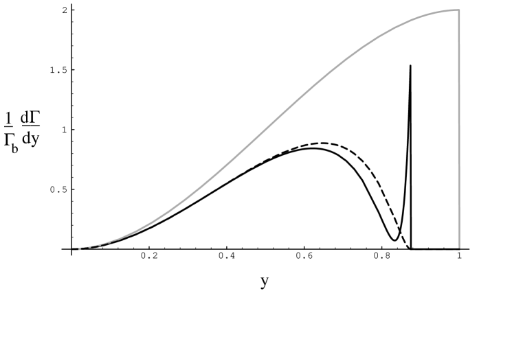
Figure 1: The electron spectrum for free quark $b\rightarrow c$ decay (dashed line), free quark $b\rightarrow u$ decay (grey line), and $B\rightarrow X_{c}e\bar{\nu}_{e}$ decay including $1/m_{b}^{2}$ corrections (solid line) with $\lambda_{1}=-0.5$ GeV² and $\lambda_{2}=0.12$ GeV². The figure is from [8].

Figure 1 shows the distributions for inclusive semileptonic decays of $B$ mesons. The spectrum close to the endpoint, where the lepton energy becomes maximal, exhibits a sharp spike as $y\to y_{max}$. Close to the endpoint we have

$$\frac{1}{\Gamma_{b}}\frac{d\Gamma}{dy}\sim 2\Theta(1-y-\rho)$$ (44)

$$\times\left[\frac{\lambda_{1}}{(m_{Q}(1-y))^{2}}\left(\frac{\rho}{1-\rho}\right)^{2}\left\{3-4\left(\frac{\rho}{1-\rho}\right)\right\}\right]$$

where $\rho=m_{c}^{2}/m_{b}^{2}$. This expression behaves like $\delta$-functions and its derivatives as $\rho\to 0$, which can be seen in (43). This behaviour indicates a breakdown of the operator product expansion close to the endpoint, since for the spectra the expansion parameter is not $1/m_{Q}$, but rather $1/(m_{Q}-qv)$, which becomes $1/(m_{Q}[1-y])$ after the integration over the neutrino momentum. In order to obtain a description of the endpoint region, one has to perform some resummation of the operator product expansion.

3.3 The Endpoint Region $E_{\ell}\sim E_{max}$

Very close to the endpoint of the inclusive semileptonic decay spectra only a few resonances contribute. In this resonance region one may not expect to have a good description of the spectrum using an approach based on parton-hadron duality; here a sum over a few resonances will be appropriate.

In the variable $y$ the size of this region is however of the order of $(\bar{\Lambda}/m_{Q})^{2}$ and thus small. In a larger region of the order $\bar{\Lambda}/m_{Q}$, which we shall call the endpoint region, many resonances contribute and one may hope to describe the spectrum in this region using parton-hadron duality.

It has been argued in [29] that the $\delta$-function-like singularities appearing in (43) may be reinterpreted as the expansion of a non-perturbative function describing the spectrum in the endpoint region. Keeping only the singular terms of (43) we write

$$\frac{1}{\Gamma_{b}}\frac{d\Gamma}{dy}=2y^{2}(3-2y)S(y),$$ (45)

where

$$S(y)=\Theta(1-y)+\sum_{n=0}^{\infty}a_{n}\delta^{(n)}(1-y)$$ (46)

is a non-perturbative function given in terms of the moments of the spectrum, taken over the endpoint region. These moments themselves have an expansion in $1/m_{Q}$ such that $a_{n}\sim 1/m_{Q}^{n+1}$, and we shall consider only the leading term in the expansion of the moments, corresponding to the most singular contribution to the endpoint region.

Comparing (43) with (45) and (46) one obtains that

$$a_{0} = \int dy(S(y)-\Theta(1-y))=0$$ (47)

$$a_{1} = \int y(S(y)-\Theta(1-y))=-\frac{\lambda_{1}}{3m_{Q}^{2}}$$ (48)

where the integral extends over the endpoint region.

The non-perturbative function implements a resummation of the most singular terms contributiong to the endpoint and, in the language of deep inelastic scattering, corresponds to the leading twist contribution. This resummation has been studied in QCD [30, 18] and the function $S(y)$ may be related to the distribution of the light cone component of the heavy quark residual momentum inside the heavy meson. The latter is a fundamental function for inclusive heavy-to-light transitions, which has been defined in [18]

$$f(k_{+})=\frac{1}{2m_{B}}\langle B(v)|\,\bar{h}_{v}\,\delta(k_{+}-iD_{+})\,h_{v}\,|B(v)\rangle,$$ (49)

where $k_{+}=k_{0}+k_{3}$ is the positive light cone component of the residual momentum $k$. The relation between the two functions $S$ and $f$ is given by

$$S(y)=\frac{1}{m_{Q}}\int\limits_{-m_{Q}(1-y)}^{\bar{\Lambda}}dk_{+}f(k_{+})$$ (50)

from which we infer that the $n^{th}$ moment of the endpoint region is given in terms of the matrix element $\langle B(v)|\bar{h}_{v}(iD_{+})^{n}h_{v}|B(v)\rangle$.

The function $f$ is a universal distribution function, which appears in all heavy-to-light inclusive decays; another example is the decay $B\to X_{s}\gamma$ [31, 18], where this function determines the photon-energy spectrum in a region of order $1/m_{Q}$ around the $K^{*}$ peak.

Some of the properties of $f$ are known. Its support is $-\infty<k_{+}<\bar{\Lambda}$, it is normalized to unity, and its first moment vanishes. Its second moment is given by $a_{1}$, and its third moment has been estimated [18, 25]. A one-parameter model for $f$ has been suggested in [30], which incorporates the known features of $f$

$$f(k_{+})={32\over\pi^{2}\bar{\Lambda}}\,(1-x)^{2}\exp\bigg{\{}-{4\over\pi}\,(1-x)^{2}\bigg{\}}\,\Theta(1-x),$$ (51)

where $x=k_{+}/\bar{\Lambda}$, and the choice $\bar{\Lambda}=570$ MeV yields reasonable values for the moments. In fig. 2 we show the spectrum for $B\to X_{u}\ell\nu_{\ell}$ using the ansatz (51).

Figure 2: Charged-lepton spectrum in $B\to X_{u}\ell\bar{\nu}$ decays. The solid line is (45) with the ansatz (51), the dashed line shows the prediction of the free-quark decay model. The figure is from [30].

Including the non-perturbative effects yields a reasonably behaved spectrum in the endpoint region and the $\delta$-function-like singularities have disappeared. Furthermore, the spectrum now extends beyond the parton model endpoint; it is shifted from $E_{\ell}^{max}=m_{b}/2$ to the physical endpoint $E_{\ell}^{max}=M_{B}/2$, since $f$ is non-vanishing for positive values of $k_{+}<\bar{\Lambda}=M_{B}-m_{b}$.

3.4 Inclusive Non-leptonic and Rare Decays

The same method as described above for the semileptonic decays has been applied to rare [10] and also to non-leptonic decays, see [32] for a recent review. For simplicity we shall restrict the discussion here to a few simple examples.

The effective Hamiltonian for the radiative rare decays $B\to X_{s}\gamma$ is given by (32) with

$$R=-\frac{4G_{F}}{\sqrt{2}}C_{7}(m_{b})\frac{e}{32\pi^{2}}m_{b}\,\,\sigma^{\mu\nu}(1+\gamma_{5})s\,F_{\mu\nu},$$ (52)

where $C_{7}(\mu)$ is a coefficient calculated e.g. in [33].

Going through the steps outlined above, one obtains for the inclusive rate of $B\to X_{s}\gamma$, including the first non-perturbative correction [10]

$$\Gamma_{B\to X_{s}\gamma}=\frac{\alpha G_{F}^{2}}{16\pi^{4}}m_{b}^{5}|V_{ts}V_{td}^{*}|^{2}|C_{7}(m_{b})|^{2}\left[1+\frac{1}{2m_{b}^{2}}\left(\lambda_{1}-9\lambda_{2}\right)\right].$$ (53)

Along the same lines one may study the inclusive decays $B\to X_{s}\ell^{+}\ell^{-}$, the results for the lepton spectra and the total rates may be found in [10].

Similarly one may consider the total rates for inclusive non-leptonic decays. Neglecting for simplicity penguin contributions and CKM-suppressed decay modes, the effective Hamiltonian is given by

$$H_{eff}=\frac{G_{F}}{\sqrt{2}}\left(C_{1}(\mu)O_{1}(\mu)+C_{2}(\mu)O_{2}(\mu)\right)$$ (54)

with the two operators

$$O_{1}=\{\bar{b}\gamma_{\mu}(1-\gamma_{5})c\}\{\bar{u}\gamma_{\mu}(1-\gamma_{5})d\},$$ (55)

$$O_{2}=\{\bar{b}\gamma_{\mu}(1-\gamma_{5})d\}\{\bar{u}\gamma_{\mu}(1-\gamma_{5})c\},$$ (56)

where the braces denote the coupling to colour singlet, and the $C_{j}$ are the corresponding Wilson coefficients, which may be found e.g. in [34].

From this one obtains for the inclusive width for $B\to X_{c}$ [32]

$$\Gamma_{B\to X_{c}}=\frac{G_{F}^{2}m_{b}^{5}}{64\pi^{3}}\left\{A_{1}f_{1}\left(\frac{m_{c}}{m_{b}}\right)\left[1+\frac{1}{2m_{b}^{2}}(\lambda_{1}-9\lambda_{2})\right]-48A_{2}f_{3}\left(\frac{m_{c}}{m_{b}}\right)\frac{1}{2m_{b}^{2}}\lambda_{2}\right\},$$ (57)

where $A_{1/2}$ is a combination of Wilson coefficients appearing in the effective Hamiltonian

$$A_{1}=C_{1}^{2}(m_{b})+C_{2}^{2}(m_{b})+\frac{2}{3}C_{1}(m_{b})C_{2}(m_{b})$$ (58)

$$A_{2}=\frac{2}{3}C_{1}(m_{b})C_{2}(m_{b}),$$

and $f_{1}$ and $f_{3}$ are phase-space factors; $f_{1}$ is defined in (40), while $f_{3}$ is

$$f_{3}(x)=(1-x^{2})^{3}.$$ (59)

Equation(57) is a QCD-based calculation of the inclusive non-leptonic width, and together with the corresponding expression for the semileptonic width (38) it gives us the lifetime of bottom hadrons and their semileptonic branching fraction, including the non-perturbative corrections in a $1/m_{Q}$ expansion. However, before one may compare the results with data, one has to take into account perturbative QCD corrections as well. These corrections have been calculated and are presented in a contribution to this conference [36].

4 Concluding Remarks

The expansion of QCD in inverse powers of the heavy-quark mass has put heavy-quark physics on a model-independent basis. In particular, the symmetries present in the heavy quark limit allow a variety of model-independent predictions for weak decay matrix elements. For mesons, the Isgur–Wise function (22) is the only non-perturbative input in the heavy mass limit.

However, the corrections of order $\bar{\Lambda}/m_{Q}$ introduce in general new form factors, i.e. an additional non-perturbative input is needed. Still a few relations, like the normalization of certain form factors, are do not receive linear corrections, and the first subleading contribution is of order $(\bar{\Lambda}/m_{Q})^{2}$. For $m_{Q}=m_{c}=1.5$ GeV and for $\bar{\Lambda}=500$ MeV this gives a typical size of corrections in the ballpark of 10%, which is what is found, for example for the normalization of the form factor relevant for the $V_{cb}$ determination. In general, these corrections will be the final limitation for model-independent statements from HQET.

These remarks apply in particular to the determination of $V_{cb}$ from the exclusive channel $B\to D^{*}\ell\nu_{\ell}$, where the theoretical errors quoted above is about 6% and dominated by the uncertainties of the estimates of the $1/m_{Q}^{2}$ contributions, which need model input. This has to be compared with the determination of $V_{cb}$ from inclusive decays, which has been discussed in detail in [26]. The inclusive width in the framework discussed above depends on the quark masses, and superficially one finds a $m_{Q}^{5}$ dependence. This would mean that even small uncertainties in the heavy-quark mass would have a large effect on a $V_{cb}$ determination based on the inclusive width. However, it has been argued in [26] that the inclusive decays $B\to X_{c}\ell\nu$ will receive their major contribution from the kinematic region close to the non-recoil point; in this region the inclusive width depends almost linearly only on the mass difference $m_{b}-m_{c}$ with only a weak dependence on $m_{b}+m_{c}$. The quark-mass difference is much better known than the individual masses; using the mass formula (15) only $\lambda_{1}$ enters. Based on these observations it has been argued in [26] that a determination of $V_{cb}$ from inclusive decays may have a theoretical error of as low as 5%; the uncertainty here enters through the parameter $\lambda_{1}$, which is at present only poorly known, but may be measured in the future from the inclusive semileptonic decay spectra [37]. Given the present situation both methods have comparable theoretical uncertainties and it remains to be seen for which of the two methods the uncertainties appearing at order $1/m_{Q}^{2}$ will be better under control.

Although there has been some theoretical progress in setting up a QCD-based calculation for inclusive widths, non-leptonic decays still remain a problem. It has been noticed soon after the formulation of the $1/m_{Q}$ expansion for inclusive non-leptonic processes that the non-perturbative effects calculated in this way are small, too small to explain the experimental data on the inclusive semileptonic branching fraction of $B$ mesons. However, there are perturbative corrections as well, which have been calculated recently, taking into account a non-zero mass for the quarks in the final state [35, 36]. These corrections are substantial only in the channel $b\to\bar{c}cs$ and hence yield an enhancement charm production in $B$ decays that is not supported by present data. Thus the problem of the semileptonic branching fraction still persists.

The difficulty seems to be the calculation of the inclusive non-leptonic width, and not the semileptonic one. This is supported by another problem, which is the lifetime of the $\Lambda_{b}$ baryon. Based on the $1/m_{Q}$ expansion one would conclude that the $\Lambda_{b}$ lifetime should be slighly smaller than the $B$ meson lifetime, $\tau_{\Lambda_{b}}\sim 0.9\tau_{B}$ [32]. This is not supported by recent data, indicating that $\tau_{\Lambda_{b}}\sim 0.7\tau_{B}$ where the experimental error is 15% [38]. The situation in the charm system is even worse, here the lifetime differences are substantial, $\tau_{\Lambda_{c}}\sim 0.5\tau_{D^{0}}$ and $\tau_{\Lambda_{c}}\sim 0.2\tau_{D^{\pm}}$. This indicates that the $1/m_{Q}$ expansion for inclusive non-leptonic decays is not yet understood and the problems have been recently summarized in [39]. Unlike exclusive non-leptonic decays, which still may be described only in a model framework, the description of inclusive non-leptonic decays is based on QCD and the above problems certainly deserve further study.

References

- [1] M. Voloshin and M. Shifman, Sov. J. Nucl. Phys. 45 (1987) 292 and 47 (1988) 511; E. Eichten and B. Hill, Phys. Lett. B234 (1990) 511; a more complete set of references can be found in one of the reviews [3].
- [2] N. Isgur and M. Wise, Phys. Lett. B232 (1989) 113 and B237 (1990) 527; B. Grinstein, Nucl. Phys. B339 (1990) 253; H. Georgi, Phys. Lett. B240 (1990) 447; A. Falk, H. Georgi, B. Grinstein and M. Wise, Nucl. Phys. B343 (1990) 1.
- [3] H. Georgi: contribution to the Proceedings of TASI–91, by R. K. Ellis et al. (eds.) (World Scientific, Singapore, 1991); B. Grinstein: contribution to High Energy Phenomenology, R. Huerta and M. A. Peres (eds.) (World Scientific, Singapore, 1991); N. Isgur and M. Wise: contribution to Heavy Flavors, A. Buras and M. Lindner (eds.) (World Scientific, Singapore, 1992); M. Neubert, SLAC–PUB 6263 (1993) (to appear in Phys. Rep.); T. Mannel, contribution to QCD–20 years later, P. Zerwas and H. Kastrup (eds.) (World Scientific, Singapore 1993).
- [4] M. Shifman and M. Voloshin, Sov. J. Nucl. Phys. 41 (1985) 120; V. Khoze et al., Sov. J. Nucl. Phys. 46 (1987) 112.
- [5] J. Chay, H. Georgi and B. Grinstein, Phys. Lett. B247 (1990) 399.
- [6] I. Bigi, N. Uraltsev and A. Vainshtein, Phys. Lett. B293 (1992) 430; I. Bigi et al., Minnesota TPI-MINN-92/67-T (1992) and Phys. Rev. Lett. 71 (1993) 496.
- [7] B. Blok et al., Phys. Rev. D49 (1994) 3356.
- [8] A. Manohar and M. Wise, Phys. Rev. D49 (1994) 1310.
- [9] T. Mannel, Nucl. Phys. B423 (1994) 396.
- [10] A. Falk, M. Luke and M. Savage, Phys. Rev. D49 (1994) 3367.
- [11] T. Mannel, W. Roberts and Z. Ryzak, Nucl. Phys. B 368 (1992) 204.
- [12] M. Luke and A. Manohar, Phys. Lett. B286 (1992) 348; Y. Chen, Phys. Lett. B317 (1993) 421.
- [13] A. Falk, B. Grinstein and M. Luke, Nucl. Phys. B 357 (1991) 185.
- [14] Y. Chen, Y. Kuang and R. Oakes, preprint NSF-ITP-94-49, hep-ph/9406287 (1994).
- [15] N. Isgur and M. Wise, Nucl. Phys. B348 (1991) 276; H. Georgi, Nucl. Phys. B348 (1991) 293; T. Mannel, W. Roberts and Z. Ryzak, Nucl. Phys. B355 (1991) 38.
- [16] A. Falk, Nucl. Phys. B 378 (1992) 79.
- [17] M. Beneke and V. Braun, Munich preprint MPI-PHT-94-9 (1994), hep-ph/9402364; I.I. Bigi et al., Minnesota preprint TPI-MINN-94-4-T (1994), hep-ph/9402360; M. Neubert and C. Sachrajda, preprint CERN-TH-7312-94 (1994), hep-ph/ 9407394; M. Luke, A. Manohar and M. Savage, Toronto preprint UTPT-94-21 (1994); hep-ph/9407407.
- [18] I. Bigi et al., Int. J. Mod. Phys. A9 (1994) 2467.
- [19] I. Bigi et al., preprint CERN-TH-7250/94 (1994), hep-ph/9405410.
- [20] P. Ball and V. Braun, Phys. Rev. D49 (1994) 2472.
- [21] M. Neubert, contribution to this conference.
- [22] M. Ademollo and R. Gatto, Phys. Rev. Lett. 13 (1964) 264.
- [23] M. Luke, Phys. Lett. B252 (1990) 447.
- [24] A. Falk and M. Neubert, Phys. Rev. D47 (1993) 2965.
- [25] T. Mannel, Phys. Rev. D50 (1994) 428.
- [26] M. Shifman, N. Uraltsev and A. Vainshtein, Minnesota preprint TPI-MINN-94-13-T (1994), hep-ph/9405207.
- [27] M. Neubert, preprint CERN-TH-7395-94 (1994), hep-ph/9408290.
- [28] A. Ali and E. Pietarinen, Nucl. Phys. B154 (1979) 519; N. Cabibbo, G. Corbo and L. Maiani, Nucl. Phys. B155 (1979) 83; G. Altarelli et al., Nucl. Phys. B208 (1982) 365; G. Corbo, Nucl. Phys. B212 (1983) 99; M. Jezabek and J. H. Kühn, Nucl. Phys. B320 (1989) 20; A. Falk et al., Phys. Rev. D49 (1994) 3367.
- [29] M. Neubert, Phys. Rev. D49 (1994) 2472.
- [30] T. Mannel and M. Neubert, preprint CERN-TH.7156/94 (1994).
- [31] M. Neubert, Phys. Rev. D49 (1994) 4623.
- [32] I. Bigi et al. preprint CERN-TH-7132-94 (1994). to appear in 2nd ed. of B Decays, S. Stone (ed.), World Scientific, Singapore.
- [33] B. Grinstein, R. Springer and M. Wise, Nucl. Phys. B319 (1988) 271; M. Misiak, Nucl. Phys. B393 (1993) 23.
- [34] F. Gilman and M. Wise, Phys. Rev. D20 (1979) 2392; A. Buras et al., Nucl. Phys. B370 (1992) 69.
- [35] E. Bagan et al., Munich preprint TUM-T31-67-94 (1994), hep-ph/9408306.
- [36] P. Ball, contribution to this conference.
- [37] I. Bigi et al., Minnesota preprint TPI-MINN-94-25-T (1994), hep-ph/9407296.
- [38] ALEPH Collaboration, contribution to the ICHEP94 Conference, Glasgow, 1994.
- [39] A. Falk, M. Wise and I. Dunietz, Caltech preprint CALT-68-1933 (1994), hep-ph/9405346.