July 1994 MITH 94/10 Higher Twist, Polarised Structure Functions
and the Bjorken System of Equations

Abstract

We discuss the present situation with regard to polarised nucleon structure function measurements. In particular we examine the status of the Bjorken sum rule in the light of the recent data on the spin structure functions of (i) the deuteron obtained by the SMC group at CERN and (ii) the neutron by the E142 group at SLAC. In order to fully exploit all the available data it is necessary to study the complete Bjorken system of equations, which may be done in any of several equivalent ways. Combining the new data with that already obtained for the proton by the EMC group and earlier SLAC/YALE collaborations, together with bounds obtained on the strange quark polarisation, we show that the Bjorken system of equations is violated at about the $2\sigma$ level. We also show, using unpolarised data, that arguments based on possible higher-twist contributions are unable to account for this discrepancy. In conclusion, a simple explanation in terms of a non-perturbative renormalisation of the relevant Wilson coefficients is presented.
PACS: 13.88.+e, 13.60.Hb, 12.38.Qk

1 Introduction

It has long been held (albeit by a limited community of “spin physicists”) that polarised deep-inelastic scattering (DIS) can provide very stringent tests of factorisation in perturbative QCD (PQCD) and the quark-parton model (QPM). Indeed, polarisation effects in general provide valuable insight into the dynamics of hadronic interactions and are extremely sensitive to the bound-state structure, so elusive to theoretical approaches [(1)]. In particular, the Bjorken sum rule (BSR) [(2), (3)] is a measurable quantity that can be used for comparison between experimental data and theoretical predictions. The experimental precision attainable now surpasses the ten-percent level while, on the theoretical side, all relevant PQCD calculations have been carried out to at least two-loop order (i.e., one-percent level) and for the BSR itself to three loops [(26)]. Thus, one can consider such comparisons as serious, indeed obligatory, tests of the applicability of PQCD to such processes.

Like many other sum rules, the BSR is a direct consequence of the operator-product expansion, as applied to DIS and justified by asymptotic freedom in PQCD. In simple terms, all DIS structure-function sum rules may be derived from the hypothesized point-like behaviour of strong interactions at short distances. However, only the Adler sum rule [(4)] is directly associated with a conserved hadronic current and is therefore unique in not receiving higher-order PQCD corrections, i.e., the Wilson coefficient associated with the relevant light-cone operator is unity to all orders in (and is independent of) perturbation theory. That is, the validity of the Adler sum rule is not actually dependent on the validity of PQCD, being founded on symmetry principles of a deeper level, and its violation is virtually inconceivable in the present field-theoretic framework. In contrast, the Wilson coefficients associated with both the BSR and Gross-Llewellyn Smith sum rule [(5)] are $1{-}\frac{\alpha_{S}}{\pi}$ (to first or next-to-leading logarithmic order); consequently, both sum rules are inextricably linked to perturbation theory and any discrepancy between their prediction and measurement should be taken as evidence for a failure of PQCD in predicting the normalisation of the Wilson coefficients.

2 Polarised Deep-Inelastic Scattering

By performing DIS with both beam and target polarised longitudinally, access is gained to the structure function $g_{1}(x,Q^{2})$ [(6)]. In the QPM this structure function has a simple relation to polarised quark distributions, analogous to that of $F_{1}(x,Q^{2})$:

$$\begin{array}[]{r@{\;=\;}l}g_{1}(x,Q^{2})&\mbox{$\frac{1}{2}$}\sum_{f}e_{f}^{2}\,\Delta q_{f}(x,Q^{2}),\\ F_{1}(x,Q^{2})&\mbox{$\frac{1}{2}$}\sum_{f}e_{f}^{2}\,q_{f}(x,Q^{2}),\end{array}$$ (1)

where the sum runs over quarks and antiquarks of flavour $f$, $e_{f}$ is the $f$-quark fractional charge and $x$ is the usual Bjorken scaling variable or momentum fraction of the struck quark. The quark densities are defined in the following manner:

$$\begin{array}[]{r@{\;=\;}l}\Delta q_{f}(x,Q^{2})&q_{f}^{+}(x,Q^{2})-q_{f}^{-}(x,Q^{2}),\\ q_{f}(x,Q^{2})&q_{f}^{+}(x,Q^{2})+q_{f}^{-}(x,Q^{2}),\end{array}$$ (2)

where $q_{f}^{\pm}(x,Q^{2})$ are the densities of quarks of flavour $f$ and positive or negative helicity with respect to that of the parent hadron.

Of course, experimentally it is an asymmetry that is actually measured: namely, the ratio of the difference and sum of cross-sections for opposite helicity configurations. The polarised structure function is then extracted, using the following working definition:

$$g_{1}(x,Q^{2})=\frac{A_{1}(x,Q^{2})\,F_{2}(x,Q^{2})}{2x\,(1+R(x,Q^{2}))},$$ (3)

where $R_{1}(x,Q^{2})$ is the usual ratio of longitudinal to transverse unpolarised structure functions and $A_{1}(x,Q^{2})$ is the measured asymmetry.

Sum rules equate integrals over $x_{B}$ of such structure functions to independently known quantities. For example, using SU(2) current algebra and assuming scale invariance, Bjorken showed [(2), (3)] that the proton-neutron difference for $g_{1}$ was given by the axial-vector $\beta$-decay constant of the neutron, $g_{A}$:

$$\Gamma_{1}^{p-n}=\int_{0}^{1}dx\,g_{1}^{p-n}(x,Q^{2})=\mbox{$\frac{1}{6}$}\,g_{A}.$$ (4)

Note that here there is apparently no longer any dependence on the energy scale, $Q^{2}$. In fact, in PQCD there are radiative corrections to the right-hand side that depend on the running coupling constant $\alpha_{S}(Q^{2})$ and thus only a logarithmic variation of the (experimental) left-hand side is expected at most. This sum rule therefore becomes a rigorous prediction of PQCD, through the justification of asymptotic freedom that leads to an approximate scaling behaviour.

3 The Bjorken System of Equations

The BSR, first dismissed as worthless [(2)] but later revalued [(3)], is nevertheless difficult to test; it requires a precision measurement of $g_{1}$ for both the proton and neutron over a sizeable range of $x_{B}$ (roughly speaking, a coverage of $0.01{<}x{<}0.6$ is necessary). While precise data have been available for the former target since 1988 [(7), (8)], the first ever data for the latter have only recently been published [(9), (10), (11), (12)]. Moreover, the full SU(3) algebra of the baryon octet actually admits three independent quantities, which, while having their natural expression in terms of up, down and strange quarks, are better expressed in terms of the SU(3) axial-vector couplings:

$$\begin{array}[]{c@{\;=\;}l}\langle\,p^{\uparrow}\,|\;\bar{u}\gamma_{3}\gamma_{5}u-\bar{d}\gamma_{3}\gamma_{5}d\;|\,p^{\uparrow}\,\rangle&g_{A},\\ \langle\,p^{\uparrow}\,|\;\bar{u}\gamma_{3}\gamma_{5}u+\bar{d}\gamma_{3}\gamma_{5}d-2\bar{s}\gamma_{3}\gamma_{5}s\;|\,p^{\uparrow}\,\rangle&\tilde{g}_{A},\\ \langle\,p^{\uparrow}\,|\;\bar{u}\gamma_{3}\gamma_{5}u+\bar{d}\gamma_{3}\gamma_{5}d+\bar{s}\gamma_{3}\gamma_{5}s\;|\,p^{\uparrow}\,\rangle&g_{0}.\end{array}$$ (5)

The right-hand sides of the first two equations above correspond to known constants ($g_{A}{=}1.2573{\pm}0.0028$ [(13)] and $\tilde{g}_{A}{=}0.629{\pm}0.039$ [(14)]), but the third ($g_{0}$), corresponding to the flavour-singlet axial-vector current, is unknown. Thus an immediate prediction for, say, just the proton integral is not possible.

Let us remark in passing that a further combination of the $u$, $d$ and $s$ axial-current matrix elements is, in fact, accessible in $\nu$-$p$ elastic scattering [(15)] and this would in principle allow an exact prediction for single nucleon targets. Unfortunately, the precision of such measurements is still too poor to permit any strong statement.

Good arguments can be made, however, for setting the strange-quark matrix element equal to zero [(16)]: there are very few strange quarks in the proton and they are concentrated below $x_{B}{\simeq}0.1$, where all correlations are expected to have died out. Therefore the second two matrix elements of eq. (5) were expected to be equal, thus leaving only two independent quantities. This allows predictions to be made for the proton and neutron separately, which can now be expressed in terms of the two axial-vector constants and the strange-quark matrix element as

$$\Gamma_{1}^{p(n)}=(-)\mbox{$\frac{1}{12}$}g_{A}+\mbox{$\frac{5}{36}$}\tilde{g}_{A}+\mbox{$\frac{1}{3}$}\langle\,p^{\uparrow}\,|\;\bar{s}\gamma_{3}\gamma_{5}s\;|\,p^{\uparrow}\,\rangle,$$ (6)

For clarity, the PQCD corrections have been suppressed in the above, for more complete expressions see, e.g., ref. 17. Conversely, these equations may be used to extract the value of the strange-quark matrix element given the value of $\Gamma_{1}$ for either nucleon, or (as in the case of the SMC) the deuteron.

4 The Data — New and Old

We shall now compare the experimental results obtained by the three experiments with the theoretical predictions based on the Ellis-Jaffe sum rule Ellis74 :

$$\makebox[56.9055pt][l]{EMC}\Gamma_{1}^{p} = \hphantom{-}0.126\pm 0.010\pm 0.015$$

$$\makebox[56.9055pt][l]{SMC}\Gamma_{1}^{d} = \hphantom{-}0.023\pm 0.020\pm 0.015$$ (7)

$$\makebox[56.9055pt][l]{E142}\Gamma_{1}^{n} = -0.022\pm 0.006\pm 0.009$$

$$\Gamma_{1}^{p} = \hphantom{-}0.176\pm 0.006+\mbox{$\frac{1}{3}\int$}\Delta{s}$$

$$\makebox[0.0pt][l]{\raisebox{8.0pt}[0.0pt][0.0pt]{Ellis-}}\makebox[56.9055pt][l]{\raisebox{-8.0pt}[0.0pt][0.0pt]{Jaffe }}\Gamma_{1}^{d} = \hphantom{-}0.080\pm 0.006+\mbox{$\frac{1}{3}\int$}\Delta{s}$$ (8)

$$\Gamma_{1}^{n} = -0.016\pm 0.006+\mbox{$\frac{1}{3}\int$}\Delta{s}$$

The short-fall in the EMC proton measurement with respect to the Ellis-Jaffe prediction (taking ${\int}\Delta{s}{=}0$) is immediately obvious. This observation led to the coining of the phrase Spin Crisis. A similar (though less striking) observation may be made for the SMC deuteron integral. In contrast, the neutron sum rule appears well satisfied by the E142 data. In terms of the strange-quark contribution, both the EMC and SMC measurements imply ${\int}\Delta{s}{\simeq}{-}0.15$ while that of E142 leads to ${\int}\Delta{s}{\simeq}{-}0.02$. Thus an important question is immediately raised: “How big can ${\int}\Delta{s}$ be?” This is the subject of the next section.

Before moving on, let us make a few remarks on the SMC data: unfortunately, the errors are so large that they have little impact on any analysis although, taken at face value, they appear to agree with the BSR when combined with the EMC data. However, a certain neglect of these data can be motivated as follows. The particularly low value of the SMC deuteron integral is due, in roughly equal measure, to the large negative values reported at low $x$ and to the very early drop at large values of $x$. While the low-$x$ data are (barely) compatible with the smooth extrapolation to zero of the E142 data, the converse is certainly not true. Nevertheless, attempts of doubtful validity at combining the two data sets data have been made; the result is agreement with the BSR and (surprisingly) larger errors than the E142 data alone. This last fact clearly underlines the lack of statistical correctness of such a procedure. With regard to the high-$x$ region, we have shown Prep93b that the SMC data violate a rigorous bound that may be constructed from the combined EMC and unpolarised $F_{2}^{p,n}$ data; the spin data is used to eliminate the $u$-quark spin density and the $F_{2}^{p,n}$ data then bounds that of the remaining $d$-quark via positivity. Much of this discussion will be clarified by the planned E142 neutron measurements down to $x{\simeq}0.01$, using a higher beam energy.

5 Bounding the Strange-Quark Spin

Positivity trivially implies $|{\int}\Delta{s}(x)|{\leq}s(x)$, although we stress that equality would imply 100% polarisation. Now, Regge phenomenology tells us that the dominant contribution of the sea is is that of the pomeron (behaving as $x^{-1}$), which we recall is spin independent. We have used the very precise data on the unpolarised strange-quark distributions CCFR92 to bound the non-diffractive contribution and thus too the strange-quark polarisation Prep88 ; Prep90a ; Prep91a . The result of this analysis is the following bound:

$$\left|\int\Delta s\right|\leq 0.021\pm 0.001,$$ (9)

which has been challenged (e.g., see refs. 24; 25) with various proposed constructions and/or parametrisations. However, we have shown in the papers cited above that all such proposals fail to agree with present experimental and phenomenological knowledge.

A quantitative measure of the discrepancy between the data and theory may be obtained by performing a one-parameter fit for the strange-quark polarisation to the data, with and without the bound, the results Prep93a are summarized in table 1.

Table 1: Results of a one-parameter fit for the strange-quark polarisation to the data, with and without the bound.

$$\begin{array}[]{|||l|||c|c|c|||}\hline\cr\hline\cr\hline\cr\mbox{Expt.~{}Info.}&\langle\,p^{\uparrow}\,|\;\bar{s}\gamma_{3}\gamma_{5}s\;|\,p^{\uparrow}\,\rangle&\chi^{2}/\mbox{DoF}&\mbox{C.L.}\\ \hline\cr\hline\cr\hline\cr\mbox{EMC+Bound}&-0.027\pm 0.019&\hphantom{0}6.8/1&0.9\%\\ \hline\cr\mbox{EMC+SMC+E142+Bound}&-0.032\pm 0.017&10.6/3&1.4\%\\ \hline\cr\mbox{EMC+SMC+E142}&-0.088\pm 0.020&\hphantom{0}6.3/2&4.3\%\\ \hline\cr\hline\cr\hline\cr\end{array}$$

6 Higher Twist and Higher-Order PQCD

Not to be forgotten, of course, are the corrections to the various sum rules; as already mentioned above, there are PQCD higher-order corrections and the possibility of higher-twist contributions (especially in the case of the E142 data) should also be considered. For the non-singlet currents the PQCD corrections are known up to order $\alpha_{S}^{3}$ Larin91 . However, since the value of $\alpha_{S}$ extracted experimentally is only valid up to order $\alpha_{S}^{2}$ we only perform the analysis to this order. Although the inclusion of the second-order contribution does indeed shift the prediction for the BSR closer to the measured value, the effect is only of the order of a few percent.

The situation with regard to higher-twist contributions requires a little more care. Ellis and Karliner Ellis93 have claimed that according to QCD sum-rule calculations Bali90 the higher-twist contributions to the BSR actually bring the prediction perfectly into line with the measured value. In a similar analysis, Close and Roberts Close93 show that extremely large higher-twist contributions are required to explain all the data simultaneously. The argument is as follows: the neutron data are taken at an average $Q^{2}$ of only $2\,\mbox{GeV}^{2}$ while the EMC data taken at an average $Q^{2}$ of $11\,\mbox{GeV}^{2}$; the problem then is to combine them at some common value of $Q^{2}$. Experimentally it has been noted by each of the groups that the asymmetry is independent of $Q^{2}$, within experimental accuracy. Thus it is reasonable to use the very precise parametrisations of $F_{2}(x,Q^{2})$ to extract $g_{1}(x,Q^{2})$ for any desired energy scale. Ellis and Karliner then propose to take the EMC data and “evolve” them down to the scale of the E142 data; it turns out that the variation in the integral of $g_{1}^{p}$ is very small. At this point it is necessary to introduce a theoretical input, in the form of the above-mentioned predictions for the higher-twist component of the BSR. Such predictions are clearly model dependent and the associated errors are typically of the order of 100%. Moreover, a recent paper Ji93 has brought to light an error in the input for these calculations, suggesting that the contribution should be rather smaller and of the opposite sign.

In any case, it is clearly preferable to try to avoid the the necessity of higher-twist estimates; this can be achieved by simply evolving the E142 data to the higher scales of the EMC experiment. It turns out, using this procedure, that the variation in the integral of $g_{1}^{n}$ is also small, reflecting a negligible higher-twist component. Thus the value of the BSR at $Q^{2}{=}11\,\mbox{GeV}^{2}$ is only slightly affected by this procedure; the integrated values for the proton, neutron and BSR at $Q^{2}{=}11\,\mbox{GeV}^{2}$ are

$$\begin{array}[]{ll@{\;=\;}c@{\,\pm\,}c}\mbox{EMC}&\Gamma_{1}^{p}&\hphantom{-}0.128&0.019\\ \mbox{E142}&\Gamma_{1}^{n}&-0.032&0.011\\ \makebox[85.35826pt][l]{BSR~{}(expt.)}&\Gamma_{1}^{p-n}&\hphantom{-}0.160&0.022\end{array}$$ (10)

to be compared with

$$\begin{array}[]{ll@{\;=\;}c@{\,\pm\,}c}\makebox[85.35826pt][l]{BSR~{}(th.)}&\Gamma_{1}^{p-n}&\hphantom{-}0.192&0.003\end{array}$$ (11)

Our results for the $Q^{2}$ dependence of the various sum rules are displayed graphically in figs. 1 and 2. In table 2 we show the result of separating the various leading- and higher-twist contributions to the sum rules via a knowledge of the $Q^{2}$ dependence of the unpolarised structure functions.

     

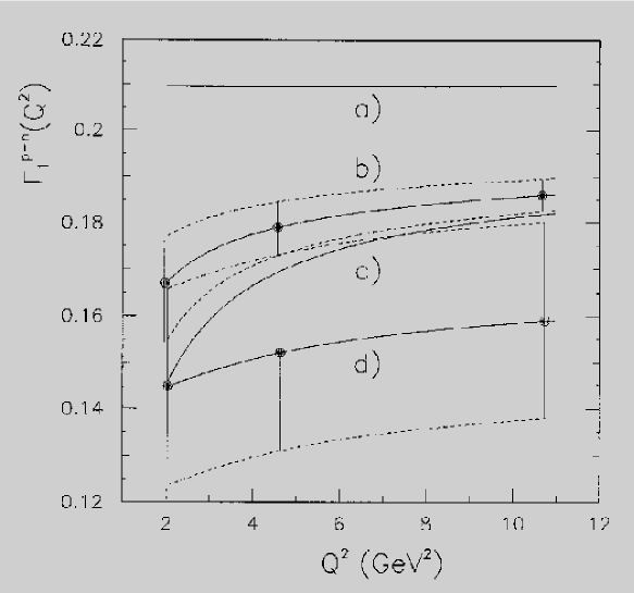
Figure 1: The solid curves are the Bjorken sum rule: a) asymptotic value, b) with the PQCD correction, c) PQCD and higher twist, d) experimental evaluation; the errors for a) and c) are given by the dashed lines.

     

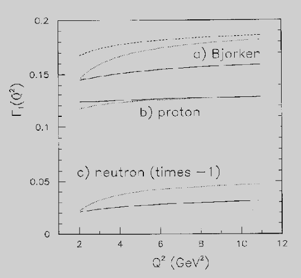
Figure 2: The experimentally evaluated sum rules, as functions of $Q^{2}$, of a) Bjorken, b) $\int_{0}^{1}g_{1}^{p}$ and c) $-\int_{0}^{1}g_{1}^{n}$ (solid curves) together with the PQCD (dashed curves) and PQCD plus higher-twist predictions (dotted curves).

Table 2: The proton and neutron integrals and higher-twist corrections, the fourth and fifth columns give the two corrections and the last column contains the corrected (i.e., leading-twist) integrals. Note that rounding errors cause slight discrepancies between the various figures.

$$\begin{array}[]{|||r|c|r|r|r|r|||}\hline\cr\hline\cr\hline\cr Q^{2}&\mbox{Target}&\Gamma_{1}^{\rm expt.}&\delta\Gamma_{1}^{\rm DHT}&\delta\Gamma_{1}^{\rm TM}&\Gamma_{1}^{\rm LT.}\\ \hline\cr\hline\cr\hline\cr&n&-0.020&-0.003&0.000&-0.023\pm 0.010\\ \cline{2-6}\cr 2.0&p&0.124&-0.005&-0.003&0.116\pm 0.017\\ \cline{2-6}\cr&p-n&0.144&-0.002&-0.002&0.140\pm 0.020\\ \hline\cr\hline\cr\hline\cr&n&-0.026&-0.001&0.000&-0.028\pm 0.010\\ \cline{2-6}\cr 4.6&p&0.125&-0.001&-0.001&0.123\pm 0.017\\ \cline{2-6}\cr&p-n&0.152&0.000&-0.001&0.151\pm 0.020\\ \hline\cr\hline\cr\hline\cr&n&-0.031&-0.001&0.000&-0.032\pm 0.010\\ \cline{2-6}\cr 10.7&p&0.128&0.000&0.000&0.127\pm 0.017\\ \cline{2-6}\cr&p-n&0.159&0.000&0.000&0.159\pm 0.020\\ \hline\cr\hline\cr\hline\cr\end{array}$$

7 Extracting Spin Densities from the Data

Adopting the attitude that the overall normalisation of the proton matrix elements of the light-cone current operators is unreliably estimated in PQCD, it might be asked if there is any way to extract the three unknowns (i.e., $\Delta{u}$, $\Delta{d}$ and $\Delta{s}$) from essentially only two independent data sets (proton and neutron). Now, while overall normalisations are often unreliable, ratios are well determined in the standard broken SU(6) picture of the nucleon; thus let us take as a reliable quantity only the ratio

$$\frac{\Delta{d_{v}}}{\Delta{u_{v}}}=-\frac{(D-F)}{2F}\simeq-\frac{1}{3},$$ (12)

where $F$ and $D$ are the usual baryon-octet $\beta$-decay constants; in SU(6) the ratio $\frac{F}{D}{=}\frac{2}{3}$, experimentally it is ${\simeq}0.6$ PGR90 . Using this relation to substitute for $\Delta{d_{v}}$ in the expressions of for $\Gamma_{1}^{p,n}$ and eliminating $\Delta{u_{v}}$ between the two, we arrive at the following relation:

$$\Gamma_{1}^{n}=-\mbox{$\frac{1}{11}$}\Gamma_{1}^{p}+\mbox{$\frac{2}{3}$}\Delta{s}.$$ (13)

In obtaining the above, we have also included the phenomenological factor-two suppression of the strange over non-strange sea (although the final numerical results are rather insensitive to the actual value used). Thus, from our bound on $\Delta{s}$ and the EMC value for $\Gamma_{1}^{p}$, we could have predicted

$$0.002\geq\Gamma_{1}^{n}\geq-0.026,$$ (14)

in rather good agreement with the SLAC data.

Alternatively, we can turn these expressions around and extract the various integrated quark spin-dependent densities, using both EMC and SLAC data:

$$\begin{array}[]{r@{\;=\;}l@{\hspace{22mm}}r@{\;=\;}l}\Delta{u_{v}}&\hphantom{-}0.72\hfil\hskip 62.59605pt&\Delta{u}&\hphantom{-}0.66\\ \Delta{d_{v}}&-0.24\hfil\hskip 62.59605pt&\Delta{d}&-0.30\\ \Delta{u_{s}}=\Delta{d_{s}}&-0.06\hfil\hskip 62.59605pt&\Delta{s}&-0.03\\[6.0pt] \lx@intercol\hfil\Delta{\Sigma}{\;=\;}\Delta{u}{+}\Delta{d}{+}\Delta{s}\;=\;&\hphantom{-}0.33\end{array}$$ (15)

(the errors on the above quantities are typically of the order of $0.02-0.03$). Notice (i) the strange-quark component is entirely compatible with the bound and (ii) the total quark spin, $\Delta{\Sigma}$, is a sizeable fraction of that of the proton. With the additional standard assumption of an extra factor of $1{-}x$ for the valence $d$ density with respect to $u$, the distributions as functions of $x$ may be obtained; the corresponding curves are shown in fig. 3.

     

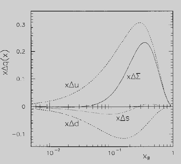
Figure 3: Our extraction of the quark spin distributions: the upper and lower dashed lines are the $u$ and $d$ quarks respectively, the dotted line is the $s$ quark and the solid line is the resulting total quark contribution.

8 Conclusions

Let us preface the closing remarks by noting that all of the above is crucially dependent on the validity of the original EMC data, which we have taken at face value. Thus, given the enormity of the conclusions to which we are ineluctably drawn, it is important to stress the urgency of remeasuring the proton spin sum rule to the highest possible precision.

Although the BSR only fails to be satisfied experimentally at something like a $1\frac{1}{2}\sigma$ level, the complete system of equations including the strange-quark polarisation bound is violated at a level of $2\frac{1}{2}\sigma$. We have also shown that a mild assumption of incorrect evaluation of the overall normalisation for hadronic matrix elements in PQCD leads to a picture of the nucleon in which a large fraction of the spin is carried by the quarks and the strange-quark spin is very small, i.e., precisely the picture existing before the beginning of the Spin Crisis.

To conclude, let us just recall that a correct prediction of the proton spin structure function had appeared in the literature Gian85 in 1985, well before the EMC results. Implicit in the ACD Fire-String model that led to this prediction, is the almost vanishing neutron spin asymmetry, as corroborated by the E142 results. The model, with an asymmetry driven essentially by a broken SU(6) symmetry, has a final-state structure in which non-physical (i.e., coloured) states are explicitly barred from contributing. The two contributions to DIS are (i) the single fire-string diagram, where quark helicity conservation makes itself strongly felt and the broken SU(6) structure leads to essentially vanishing neutron asymmetry; and (ii) the double fire-string diagram where the effects of quark polarisation are so dilute as to be negligible in all cases. The differences between the explicitly physical final-state structure of ACD and that implicitly unphysical in PQCD explain the failure of the latter to obtain the correct normalisation (or Wilson coefficients) of the nucleon matrix elements in question.

9 Note added

Since presenting this talk the next-to-leading PQCD corrections to the Ellis-Jaffe sum rule (in other words for the flavour-singlet piece) have been made available Larin94 . Thus, given the value of any single nucleon integral at some $Q^{2}$, one can perform the two-loop evolution to any desired $Q^{2}$ scale. We have checked the effect of this approach and find negligible difference with the results presented above, although it should be remarked that the theory-data discrepancy is then, in fact, slightly accentuated.

References

- (1) P.G. Ratcliffe, in Problems of Fundamental Modern Physics (World Scientific 1990, eds. R. Cherubini, P. Dalpiaz and B. Minetti), p. 233.
- (2) J.D. Bjorken, Phys. Rev. 148 (1966) 1467.
- (3) J.D. Bjorken, ibid. D1 (1970) 1376.
- (4) S.L. Adler, Phys. Rev. 143 (1966) 1144.
- (5) D. Gross and C. Llewellyn Smith, Nucl. Phys. B14 (1969) 337.
- (6) A particularly detailed and clear general review of the experimental and theoretical situation can be found in: E. Hughes, Polarized Lepton-Nucleon Scattering, presented at the 21st Annual SLAC Summer Institute (July 1993).
- (7) EMC, J. Ashman et al., Phys. Lett. B206 (1988) 364.
- (8) EMC, J. Ashman et al., Nucl. Phys. B328 (1989) 1.
- (9) SMC, B. Adeva et al., Phys. Lett. B302 (1993) 533.
- (10) M. Lowe, to appear in the proceedings of HADRON ’93 (Como, July 1993).
- (11) E142, P.L. Anthony et al., Phys. Rev. Lett. 71 (1993) 959.
- (12) G.G. Petratos, to appear in the proceedings of HADRON ’93 (Como, July 1993).
- (13) PDG, M. Anguilar-Benitez et al., Phys. Rev. D45 (1992).
- (14) P.G. Ratcliffe, Phys. Lett. B242 (1990) 271.
- (15) L.A. Ahrens et al., Phys. Rev. D35 (1987) 785.
- (16) J. Ellis and R.L. Jaffe, Phys. Rev. D9 (1974) 1444; ibid. D10 (1974) 1669.
- (17) G. Preparata and P.G. Ratcliffe, Analysis of Recent Deep-Inelastic Scattering Data Pointing to a Violation of the Bjorken Sum Rules, submitted to Phys. Rev. Lett., Milano preprint MITH 93/9.
- (18) G. Preparata and P.G. Ratcliffe, Are E142 and the SMC Telling a Different Story?, submitted to Phys. Lett. B, Milano preprint MITH 93/12.
- (19) G. Preparata and P.G. Ratcliffe, Comment on “Analysis of Data on Polarized Lepton-Nucleon Scattering”, submitted to Phys. Lett. B, Milano preprint MITH 93/15.
- (20) CCFR collab., E. Oltman et al., Z. Phys. C53 (1992) 51.
- (21) G. Preparata, and J. Soffer, Phys. Rev. Lett. 61 (1988) 1167; Erratum 62 (1989) 1213.
- (22) G. Preparata, P.G. Ratcliffe and J. Soffer, Phys. Rev. D42 (1990) 930.
- (23) G. Preparata, P.G. Ratcliffe and J. Soffer, Phys. Lett. B273 (1991) 306.
- (24) S. Brodsky, J. Ellis and M. Karliner, Phys. Lett. B206 (1988) 309.
- (25) B.L. Ioffe and M. Karliner, Phys. Lett. B247 (1990) 387.
- (26) S.A. Larin and J.A.M. Vermarseren, Phys. Lett. B259 (1991) 345.
- (27) J. Ellis and M. Karliner, Phys. Lett. B313 (1993) 131.
- (28) I.I. Balitsky, V.M. Braun and A.V. Kolesnichenko, Phys. Lett. B242 (1990) 245.
- (29) F.E. Close and R.G. Roberts, Consistent Analysis of the Spin Content of the Nucleon, Rutherford lab. preprint RAL-93-040.
- (30) X. Ji and P. Unrau, Dependence of the Proton’s Structure Function Sum Rule, submitted to Phys. Rev. Lett., MIT preprint MIT-CTP-2232.
- (31) A. Giannelli, L. Nitti, G. Preparata and P. Sforza, Phys. Lett. B150 (1985) 214.
- (32) S.A. Larin, The next-to-leading QCD approximation to the Ellis-Jaffe sum rule, CERN preprint CERN-TH.7208/94.