CERN–TH.7435/94

TUM-T31-78/94

The strange quark mass from QCD sum rules

Matthias Jamin
Theory Division, CERN, CH–1211 Geneva 23, Switzerland
and

Manfred Münz
Physik-Department, Technische Universität München
D-85747 Garching, Germany

Abstract

The strange quark mass is calculated from QCD sum rules for the divergence of the vector as well as axial-vector current in the next-next-to-leading logarithmic approximation. The determination for the divergence of the axial-vector current is found to be unreliable due to large uncertainties in the hadronic parametrisation of the two-point function.

From the sum rule for the divergence of the vector current, we obtain a value of $m_{s}\equiv\overline{m}_{s}(1\,\mbox{\rm GeV})=189\pm 32\,\mbox{\rm MeV}$, where the error is dominated by the unknown perturbative ${\cal O}(\alpha_{s}^{3})$ correction. Assuming a continued geometric growth of the perturbation series, we find $m_{s}=178\pm 18\,\mbox{\rm MeV}$. Using both determinations of $m_{s}$, together with quark-mass ratios from chiral perturbation theory, we also give estimates of the light quark masses $m_{u}$ and $m_{d}$.

CERN–TH.7435/94

TUM-T31-78/94

September 1994

1 Introduction

Quark masses are amongst the fundamental set of “a priori” unknown parameters in the standard model (SM) of particle physics. They are not physical observables, as there do not exist free quarks in nature, and hence depend on the renormalization prescription applied to the model, but have the same status as the strong QCD coupling constant $\alpha_{s}$.

In this work, we shall be concerned with a determination of the strange quark mass, $m_{s}$, at the next-next-to-leading order (NNLO) in the framework of QCD sum rules [1]. (For an overview see [2, 3, 4].) Already a considerable number of determinations of the strange quark mass can be found in the literature [5, 6, 7, 8, 9, 10, 11, 12, 13, 14, 15, 16, 17, 18, 19], however partly being incompatible within their errors. For this reason, and also because in the meantime there has been progress both on the experimental input, as well as on the theoretical expressions, we find it justified to reconsider the evaluation of $m_{s}$. In addition, there is great interest in a precise value of $m_{s}$ for the calculation of direct CP-violation in the Kaon system within the SM, because the dominant matrix elements of four-quark operators contributing to $\varepsilon^{\prime}/\varepsilon$ scale like $m_{s}^{-2}$ [20, 21].

The basic object which is investigated in the simplest version of QCD sum rules is the two-point function $\Psi(q^{2})$ of two hadronic currents

$$\Psi(q^{2})\;\equiv\;i\int\!dx\,e^{iqx}\,\big{<}\Omega|\,T\{\,j_{\Gamma}(x)\,j_{\Gamma}(0)^{\dagger}\}|\Omega\big{>}\,,$$ (1.1)

where $\Omega$ denotes the physical vacuum. To be specific, in the rest of this work $j_{\Gamma}(x)$ will be the divergence of vector and axial-vector current, $j(x)$ and $j_{5}(x)$ respectively;

$$j(x)\;=\;i\,(M-m):\!\bar{Q}(x)\,q(x)\!:\,,\qquad j_{5}(x)\;=\;i\,(M+m):\!\bar{Q}(x)\,\gamma_{5}\,q(x)\!:\,,$$ (1.2)

with $M$ and $m$ being the masses of $Q(x)$ and $q(x)$. Note that these currents are renormalization invariant operators. Throughout the paper, for notational simplicity, we shall drop the index for the pseudoscalar current, but we keep differing signs where they appear. The upper sign will always correspond to the divergence of the vector and the lower sign to the axial-vector current. It should be obvious that $\Psi(q^{2})$ is simply proportional to the two-point function of scalar (pseudoscalar) currents,

$$\Psi(q^{2})\;=\;\Big{(}M\mp m\Big{)}^{2}\,\Pi^{S,P}(q^{2})\,,$$ (1.3)

where we adopted the notation of ref. [22].

After taking two derivatives of $\Psi(q^{2})$ with respect to $q^{2}$, $\Psi^{\prime\prime}(q^{2})$ vanishes for large $q^{2}$, and satisfies a dispersion relation without subtractions (for the precise conditions see [23]):

$$\Psi^{\prime\prime}(q^{2})\;\equiv\;\frac{\partial^{2}}{(\partial q^{2})^{2}}\,\Psi(q^{2})\;=\;2\int\limits_{0}^{\infty}\frac{\rho(s)}{(s-q^{2}-i\varepsilon)^{3}}\,ds\,,$$ (1.4)

where $\rho(s)$ is defined to be the spectral function corresponding to $\Psi(s)$,

$$\rho(s)\;\equiv\;\frac{1}{\pi}\,\mbox{\rm Im}\,\Psi(s+i\varepsilon)\,.$$ (1.5)

To suppress contributions in the dispersion integral coming from higher excited states, it is further convenient to apply a Borel (inverse Laplace) transformation to eq. (1.4) which leads to

$${\cal B}_{u}\,\Psi^{\prime\prime}(q^{2})\;\equiv\;\widehat{\Psi}^{\prime\prime}(u)\;=\;\frac{1}{u^{3}}\int\limits_{0}^{\infty}e^{-s/u}\rho(s)\,ds\,,$$ (1.6)

or slightly rewriting eq. (1.6) we obtain

$$u^{3}\,\widehat{\Psi}^{\prime\prime}(u)=\int\limits_{0}^{\infty}e^{-s/u}\rho(s)\,ds\,.$$ (1.7)

As we shall discuss in detail below, the left-hand side of this equation is calculable in renormalization group improved perturbation theory, if $u$ can be chosen sufficiently large. Because the Borel transformation removes the subtraction constants in the dispersion relation and satisfies the identity

$${\cal B}_{u}\,\Psi(q^{2})\;=\;u^{2}\,{\cal B}_{u}\,\Psi^{\prime\prime}(q^{2})\,,$$ (1.8)

we could have worked directly with $\Psi(q^{2})$. To be able to investigate other types of sum rules in the future, we nevertheless prefer to express our sum rule in terms of $\Psi^{\prime\prime}(q^{2})$.

Under the crucial assumption of quark-hadron duality, the right-hand side of eq. (1.7) can be evaluated in a hadron-based picture, still maintaining the equality, and thereby relating hadronic quantities like masses and decay widths to the fundamental SM parameters. Generally, however, from experiments the phenomenological spectral function $\rho_{ph}(s)$ is only known from threshold up to some energy $s_{0}$. Above this value, we shall use the perturbative expression $\rho_{th}(s)$ also for the right-hand side. This is legitimate if $s_{0}$ is large enough so that perturbation theory is applicable. The central equation of our sum-rule analysis then is:

$$u^{3}\,\widehat{\Psi}^{\prime\prime}_{th}(u)\;=\;\int\limits_{0}^{s_{0}}e^{-s/u}\rho_{ph}(s)\,ds+\int\limits_{s_{0}}^{\infty}e^{-s/u}\rho_{th}(s)\,ds\,.$$ (1.9)

In addition, in our analysis we shall use the derivative of this equation with respect to $u$ (“first-moment sum rule”):

$$u\frac{\partial}{\partial u}\biggl{[}\,u^{3}\,\widehat{\Psi}^{\prime\prime}_{th}(u)\,\biggr{]}\;=\;\int\limits_{0}^{s_{0}}\frac{s}{u}\,e^{-s/u}\rho_{ph}(s)\,ds+\int\limits_{s_{0}}^{\infty}\frac{s}{u}\,e^{-s/u}\rho_{th}(s)\,ds\,.$$ (1.10)

In sect. 2, we give the expressions for the theoretical part of the sum rules for scalar and pseudoscalar currents at the next-next-to-leading order, and in sect. 3, the phenomenological parametrisations of the two-point functions are discussed. Sect. 4 deals with the perturbative continuum contribution and in sect. 5, we perform the numerical analysis of the sum rules. Finally, in sect. 6, we compare our results to previous determinations of $m_{s}$ published in the literature and give estimates for the light quark masses $m_{u}$ and $m_{d}$.

2 The theoretical two-point function

In the framework of the operator product expansion (OPE) [24] the two-point function (1.1) can be expanded in inverse powers of $Q^{2}\equiv-q^{2}$:

$$\Psi(Q^{2})\;=\;(M\mp m)^{2}Q^{2}\,\biggl{\{}\,\Psi_{0}+\Psi_{2}\frac{1}{Q^{2}}+\Psi_{4}\frac{1}{Q^{4}}+\Psi_{6}\frac{1}{Q^{6}}+\ldots\,\biggr{\}}\,.$$ (2.1)

The $\Psi_{n}$ contain operators of dimension $n$, and their remaining $Q^{2}$-dependence is only logarithmic. In this work, we shall treat mass like an operator of dimension 1. Otherwise, the contribution $\Psi_{2}$ would be absent because one cannot construct a gauge-invariant operator of dimension 2. Likewise, $\Psi^{\prime\prime}(Q^{2})$ has the expansion

$$\Psi^{\prime\prime}(Q^{2})\;=\;\frac{(M\mp m)^{2}}{Q^{2}}\,\biggl{\{}\,\Psi_{0}^{\prime\prime}+\Psi_{2}^{\prime\prime}\frac{1}{Q^{2}}+\Psi_{4}^{\prime\prime}\frac{1}{Q^{4}}+\Psi_{6}^{\prime\prime}\frac{1}{Q^{6}}+\ldots\,\biggr{\}}\,.$$ (2.2)

In the following sections, we shall calculate these expressions explicitly.

2.1 The perturbative contribution

In general the perturbative expression for $\Psi_{0}(Q^{2})$ is given by

$$\Psi_{0}(Q^{2})\;=\;\frac{N}{8\pi^{2}}\sum_{i=0}^{\infty}a^{i}\sum_{j=0}^{i+1}c_{ij}\,L^{j}\,,$$ (2.3)

where $N$ is the number of colours, $a\equiv\alpha_{s}/\pi$ and $L\equiv\ln(Q^{2}/\mu^{2})$. $\mu^{2}$ is a renormalization scale. Throughout this work, we shall use the modified minimal subtraction scheme ${\overline{MS}}$ [25]. From eq. (2.3), we easily obtain the corresponding expression for $\Psi_{0}^{\prime\prime}(Q^{2})$:

$$\Psi_{0}^{\prime\prime}(Q^{2})\;=\;\frac{N}{8\pi^{2}}\sum_{i=0}^{\infty}a^{i}\sum_{j=1}^{i+1}c_{ij}\,j\Big{[}\,L^{j-1}+(j-1)L^{j-2}\,\Big{]}\,.$$ (2.4)

Let us remark that the constant coefficients $c_{i0}$ have dropped out of this expression.

Because $\Psi^{\prime\prime}(Q^{2})$ is related to a physical quantity — the spectral function $\rho(s)$ — it has to satisfy a homogeneous renormalization group equation (RGE):

$$\biggl{\{}\,-2\frac{\partial}{\partial L}+\beta(a)a\frac{\partial}{\partial a}-\gamma(a)\biggl{(}M\frac{\partial}{\partial M}+m\frac{\partial}{\partial m}\,\biggr{)}\,\biggr{\}}(M\mp m)^{2}\Psi_{0}^{\prime\prime}(Q^{2})\;=\;0\,,$$ (2.5)

where $\beta(a)$ is the QCD $\beta$-function and $\gamma(a)$ is the mass anomalous dimension. In appendix B, we have collected the coefficients of $\beta(a)$ and $\gamma(a)$ in our notation. In eq. (2.5), all coefficients multiplying a certain term $a^{i}L^{j}$ have to vanish separately. From this condition one derives relations between the various $c_{ij}$ which are also given in appendix B. The independent coefficients are conveniently chosen to be the $c_{i1}$. The coefficients $c_{01}$ and $c_{11}$ can be straightforwardly calculated and are found to be

$$c_{01}\;=\;1\qquad\hbox{and}\qquad c_{11}\;=\;\frac{17}{4}\,C_{F}\,,$$ (2.6)

with $C_{F}=(N^{2}-1)/2N$. The NNLO coefficient $c_{21}$ has been calculated recently in ref. [26]. The result is

$$c_{21} = C_{F}\biggl{[}\,\biggl{(}\frac{691}{64}-\frac{9}{4}\zeta(3)\biggr{)}C_{F}+\biggl{(}\frac{893}{64}-\frac{31}{8}\zeta(3)\biggr{)}N-\biggl{(}\frac{65}{32}-\frac{1}{2}\zeta(3)\biggr{)}f\,\biggr{]}\,,$$

$$\stackrel{{\scriptstyle N=3}}{{=}} \frac{10801}{144}-\frac{39}{2}\zeta(3)-\biggl{(}\frac{65}{24}-\frac{2}{3}\zeta(3)\biggr{)}f\,,$$ (2.7)

where $f$ is the number of flavours, and $\zeta(z)$ is the Riemann $\zeta$-function. Since $\Psi^{\prime\prime}$ satisfies a homogeneous RGE, we can sum up the logarithms by choosing $\mu^{2}=Q^{2}$. Then the coupling and the masses become running quantities, evaluated at $Q^{2}$. To NNLO and $N=f=3$ this yields for $\Psi_{0}^{\prime\prime}$:

$$\Psi_{0}^{\prime\prime}\;=\;\frac{N}{8\pi^{2}}\,\biggl{[}\,1+\frac{11}{3}\,\bar{a}(Q^{2})+\biggl{(}\frac{5071}{144}-\frac{35}{2}\zeta(3)\biggr{)}\,\bar{a}(Q^{2})^{2}+{\cal O}(\bar{a}^{3})\,\biggr{]}\,.$$ (2.8)

The final step in the evaluation of the perturbative contribution to the two-point function consists in performing the Borel transformation. Unfortunately, the running coupling $\bar{a}(Q^{2})$ as well as the running masses $\overline{M}(Q^{2})$ and $\overline{m}(Q^{2})$ at NNLO are now complicated functions of $Q^{2}$, which are conventionally expanded in powers of $\ln^{-1}(Q^{2}/\Lambda^{2})$. The Borel transform of the resulting expressions cannot be given in closed form, but has to be expanded in powers of $\ln^{-1}(u/\Lambda^{2})$, or calculated numerically [27, 28].

There is a different way to obtain the Borel transform of the two-point function. Because the differential operators for the RGE and the Borel transform act on different variables, $\mu^{2}$ and $Q^{2}$ respectively, they commute [29]. We thus apply the Borel operator directly to eq. (2.4). The necessary formulae are given in appendix A. One can then easily convince oneself that the resulting expression for $(M\mp m)^{2}\widehat{\Psi}_{0}^{\prime\prime}(u)$ again satisfies a homogeneous RGE, and the logarithms can be summed up through the choice $\mu^{2}=u$. This results in the running coupling and masses being evaluated at the scale $u$. Our final expression for $\widehat{\Psi}_{0}^{\prime\prime}(u)$ is

$$\widehat{\Psi}_{0}^{\prime\prime}(u) = \frac{N}{8\pi^{2}}\,\biggl{[}\,1+\bar{a}(u)\Big{(}c_{11}+2(1-\gamma_{E})c_{12}\Big{)}$$

$$+\,\bar{a}^{2}\Big{(}c_{21}+2(1-\gamma_{E})c_{22}+(3\gamma_{E}^{2}-6\gamma_{E}-\frac{\pi^{2}}{2})c_{23}\Big{)}$$ (2.9)

$$+\,\bar{a}^{3}\Big{(}c_{31}+2(1-\gamma_{E})c_{32}+(3\gamma_{E}^{2}-6\gamma_{E}-\frac{\pi^{2}}{2})c_{33}-2(2\gamma_{E}^{3}-6\gamma_{E}^{2}-\gamma_{E}\pi^{2}+\pi^{2}+4\zeta(3))c_{34}\Big{)}\,\biggr{]}\,,$$

where $\gamma_{E}$ is the Euler constant. Here, analogously to eqs. (2.1) and (2.2), $\widehat{\Psi}^{\prime\prime}(u)$ has been expanded in inverse powers of $u$:

$$\widehat{\Psi}^{\prime\prime}(u)\;=\;\frac{(\overline{M}(u)\mp\overline{m}(u))^{2}}{u}\,\biggl{\{}\,\widehat{\Psi}_{0}^{\prime\prime}+\widehat{\Psi}_{2}^{\prime\prime}\frac{1}{u}+\widehat{\Psi}_{4}^{\prime\prime}\frac{1}{u^{2}}+\widehat{\Psi}_{6}^{\prime\prime}\frac{1}{u^{3}}+\ldots\,\biggr{\}}\,.$$ (2.10)

In our numerical analysis we have verified explicitly that our treatment of the Borel transform leads to the same result as the method of refs. [27, 28], up to differences which are of higher order.

In addition to eq. (2.1), for the first-moment sum rule of eq. (1.10) it is convenient to define the function

$$\widehat{\Phi}(u)\;\equiv\;u\,\frac{\partial}{\partial u}\,\widehat{\Psi}^{\prime\prime}(u)\,.$$ (2.11)

Expanding this function equivalently to $\widehat{\Psi}^{\prime\prime}(u)$, eq. (2.10), we obtain

$$\widehat{\Phi}_{0}(u) = -\,\frac{N}{8\pi^{2}}\,\biggl{[}\,1+\bar{a}(u)\Big{(}c_{11}-2\gamma_{E}c_{12}\Big{)}+\bar{a}^{2}\Big{(}c_{21}-2\gamma_{E}c_{22}+(3\gamma_{E}^{2}-6-\frac{\pi^{2}}{2})c_{23}\Big{)}\qquad$$ (2.12)

$$+ \,\bar{a}^{3}\Big{(}c_{31}-2\gamma_{E}c_{32}+(3\gamma_{E}^{2}-6-\frac{\pi^{2}}{2})c_{33}-2(2\gamma_{E}^{3}-12\gamma_{E}-\gamma_{E}\pi^{2}+4\zeta(3))c_{34}\Big{)}\,\biggr{]}\,.$$

To be able to estimate the uncertainty coming from the as yet unknown ${\cal O}(a^{3})$ term in the perturbative result, we have included this contribution which depends on the coefficient $c_{31}$ in the general expressions of eqs. (2.1) and (2.12), and in our numerical analysis we varied this coefficient in order to simulate a contribution from higher orders. Let us point out however, that the ${\cal O}(a^{3})$ correction cannot be included in a completely consistent way, because this would also require the four-loop coefficients of the $\beta$-function and the mass anomalous dimension, which have not yet been calculated.

2.2 Dimension 2 operators

The contribution to the dimension 2 operators can be obtained by expanding the perturbative result for the vector-current two-point function by Generalis [30] in powers of the quark masses. Then the expression for the scalar (pseudoscalar) two-point function is calculable from the Ward-identity between the vector (axial-vector) and scalar (pseudoscalar) two-point functions (see e.g. eq. (2.3) of ref. [22]). There is, however, a subtlety, because this Ward-identity involves the renormalized, non-normal-ordered quark condensate $\big{<}\bar{\psi}\psi\big{>}$. Since from a straightforward application of perturbation theory we get expressions containing the normal-ordered condensate $\big{<}\!\!:\!\bar{\psi}\psi\!:\!\!\big{>}$, we still have to subtract from Generalis result a contribution which stems from the relation between $\big{<}\bar{\psi}\psi\big{>}$ and $\big{<}\!\!:\!\bar{\psi}\psi\!:\!\!\big{>}$ [31]. This additional contribution removes mass logarithms which are present at intermediate steps of the calculation [16, 22]. For $\Psi_{2}$ we find

$$\Psi_{2}(Q^{2}) = \frac{N}{8\pi^{2}}\,\biggl{\{}\,\biggl{[}\,2L-2+aC_{F}\Big{(}-3L^{2}+8L-\frac{25}{2}+6\zeta(3)\Big{)}\,\biggr{]}\Big{(}M^{2}+m^{2}\Big{)}$$

$$\hskip 20.77051pt\pm\,\biggl{[}\,2L-4+aC_{F}\Big{(}-3L^{2}+14L-22+6\zeta(3)\Big{)}\,\biggr{]}\,Mm\,\biggr{\}}\,.$$ (2.13)

This result is in agreement with Chetyrkin et al. [32], who also performed a calculation for the vector current, but already gave expressions in terms of non-normal-ordered condensates.

From eq. (2.13) we obtain

$$\Psi_{2}^{\prime\prime}(Q^{2})\;=\;-\,\frac{N}{4\pi^{2}}\,\biggl{\{}\,\biggl{[}\,1+aC_{F}\Big{(}-3L+7\Big{)}\,\biggr{]}\Big{(}M^{2}+m^{2}\Big{)}\pm\biggl{[}\,1+aC_{F}\Big{(}-3L+10\Big{)}\,\biggr{]}\,Mm\,\biggr{\}}\,.$$ (2.14)

Proceeding for the Borel transform as in section 2.1, we finally find

$$\widehat{\Psi}_{2}^{\prime\prime}(u)\;=\;-\,\frac{N}{4\pi^{2}}\,\biggl{\{}\,\biggl{[}\,1+\bar{a}C_{F}\Big{(}4+3\gamma_{E}\Big{)}\,\biggr{]}\Big{(}\overline{M}^{2}+\overline{m}^{2}\Big{)}\pm\biggl{[}\,1+\bar{a}C_{F}\Big{(}7+3\gamma_{E}\Big{)}\,\biggr{]}\,\overline{M}\,\overline{m}\,\biggr{\}}\,,$$ (2.15)

and

$$\widehat{\Phi}_{2}(u)\;=\;\phantom{-}\,\frac{N}{2\pi^{2}}\,\biggl{\{}\,\biggl{[}\,1+\bar{a}C_{F}\biggl{(}\frac{11}{2}+3\gamma_{E}\biggr{)}\,\biggr{]}\Big{(}\overline{M}^{2}+\overline{m}^{2}\Big{)}\pm\biggl{[}\,1+\bar{a}C_{F}\biggl{(}\frac{17}{2}+3\gamma_{E}\biggr{)}\,\biggr{]}\,\overline{M}\,\overline{m}\,\biggr{\}}\,.$$ (2.16)

Again, $\widehat{\Psi}_{2}^{\prime\prime}(u)$ satisfies a homogeneous RGE which justifies the exchange of Borel transformation and renormalization group summation.

2.3 Dimension 4 operators

There are three sources of dimension 4 operators contributing to $\Psi(Q^{2})$: explicit mass corrections $\sim m^{4}$, terms originating from the quark condensate $\sim m\big{<}\bar{\psi}\psi\big{>}$ and the gluon condensate contribution $\sim\big{<}aFF\big{>}$. To the order considered, the explicit quark mass as well as the gluon condensate contribution can, for example, be taken from ref. [22]. As for the quark condensate, to NNLO we also need ${\cal O}(\alpha_{s})$ corrections. These can either be calculated directly [33], or inferred from the cancellation of mass logarithms after expressing $\big{<}\!\!:\!\bar{\psi}\psi\!:\!\!\big{>}$ through $\big{<}\bar{\psi}\psi\big{>}$ [16], yielding identical results. The explicit expressions are:

$$\Psi_{4,m^{4}} = \frac{N}{16\pi^{2}}\,\biggl{[}\,M^{4}+4M^{2}m^{2}+m^{4}+2\Big{(}M^{4}\pm 2M^{3}m\pm 2Mm^{3}+m^{4}\Big{)}L\,\biggr{]}\,,$$ (2.17)

$$\vbox{\vskip 22.76219pt}\Psi_{4,\bar{\psi}\psi} = \frac{1}{2}\,\biggl{[}\,1+aC_{F}\biggl{(}-\frac{3}{2}L+\frac{11}{4}\biggr{)}\,\biggr{]}\Big{(}\,M\big{<}\bar{Q}Q\big{>}+m\big{<}\bar{q}q\big{>}\,\Big{)}$$

$$\pm\,\biggl{[}\,1+aC_{F}\biggl{(}-\frac{3}{2}L+\frac{7}{2}\biggr{)}\,\biggr{]}\Big{(}\,m\big{<}\bar{Q}Q\big{>}+M\big{<}\bar{q}q\big{>}\,\Big{)}\,,$$ (2.18)

$$\vbox{\vskip 22.76219pt}\Psi_{4,FF} = \frac{1}{8}\,\big{<}aFF\big{>}\,.$$ (2.19)

From these expressions one can immediately obtain $\Psi_{4}^{\prime\prime}$. It is an instructive exercise to show that again $(M\mp m)^{2}\Psi_{4}^{\prime\prime}$ does satisfy the homogeneous RGE of eq. (2.5). To this end, the condensates are conveniently rewritten into renormalization group invariant condensates [34, 31]. The formulae for the renormalization group invariant condensates are collected in appendix C. In addition, to show this one needs the terms of order $\alpha_{s}m^{4}$ which can also be calculated via expanding the result by Generalis [30].

As before, the next steps are performing the Borel transformation and summing up the logarithms through the choice $\mu^{2}=u$. This leads to

$$\widehat{\Psi}_{4}^{\prime\prime}(u) = \frac{1}{2}\,\Biggl{\{}\,\frac{1}{4}\,\Omega_{4}+\frac{\gamma_{1}}{\beta_{1}}\,\bar{a}\sum_{i}\Omega^{m_{i}q_{i}}_{3}-\frac{w_{1}}{4}\sum_{i}\overline{m}_{i}^{4}$$

$$+ \biggl{[}\,1+\bar{a}C_{F}\biggl{(}\frac{11}{4}+\frac{3}{2}\gamma_{E}\biggr{)}\,\biggr{]}\Big{(}\Omega^{MQ}_{3}+\Omega^{mq}_{3}\Big{)}\pm\biggl{[}\,2+\bar{a}C_{F}\Big{(}7+3\gamma_{E}\Big{)}\,\biggr{]}\Big{(}\Omega^{mQ}_{3}+\Omega^{Mq}_{3}\Big{)}$$

$$- \biggl{\{}\,\biggl{[}\,\frac{w_{1}}{\bar{a}}+w_{1}\biggl{(}C_{F}\biggl{(}\frac{11}{4}+\frac{3}{2}\gamma_{E}\biggr{)}+w_{2}\biggr{)}-\frac{\gamma_{1}^{0}}{4}\Big{(}1-2\gamma_{E}\Big{)}\,\biggr{]}\Big{(}\overline{M}^{4}+\overline{m}^{4}\Big{)}-\gamma_{1}^{0}\overline{M}^{2}\overline{m}^{2}$$

$$\pm\,\biggl{[}\,2\frac{w_{1}}{\bar{a}}+w_{1}\biggl{(}C_{F}\Big{(}7+3\gamma_{E}\Big{)}+2w_{2}\biggr{)}+\gamma_{1}^{0}\gamma_{E}\,\biggr{]}\Big{(}\overline{M}^{3}\overline{m}+\overline{M}\overline{m}^{3}\Big{)}\,\biggr{\}}\,\Biggr{\}}\,,$$ (2.20)

and

$$\widehat{\Phi}_{4}(u) = -\,\frac{3}{2}\,\Biggl{\{}\,\frac{1}{4}\,\Omega_{4}+\frac{\gamma_{1}}{\beta_{1}}\,\bar{a}\sum_{i}\Omega^{m_{i}q_{i}}_{3}-\frac{w_{1}}{4}\sum_{i}\overline{m}_{i}^{4}$$

$$+ \biggl{[}\,1+\bar{a}C_{F}\biggl{(}\frac{13}{4}+\frac{3}{2}\gamma_{E}\biggr{)}\,\biggr{]}\Big{(}\Omega^{MQ}_{3}+\Omega^{mq}_{3}\Big{)}\pm\biggl{[}\,2+\bar{a}C_{F}\Big{(}8+3\gamma_{E}\Big{)}\,\biggr{]}\Big{(}\Omega^{mQ}_{3}+\Omega^{Mq}_{3}\Big{)}$$

$$- \biggl{\{}\,\biggl{[}\,\frac{w_{1}}{\bar{a}}+w_{1}\biggl{(}C_{F}\biggl{(}\frac{13}{4}+\frac{3}{2}\gamma_{E}\biggr{)}+w_{2}\biggr{)}-\frac{\gamma_{1}^{0}}{4}\biggl{(}\frac{1}{3}-2\gamma_{E}\biggr{)}\,\biggr{]}\Big{(}\overline{M}^{4}+\overline{m}^{4}\Big{)}-\gamma_{1}^{0}\overline{M}^{2}\overline{m}^{2}$$

$$\pm\,\biggl{[}\,2\frac{w_{1}}{\bar{a}}+w_{1}\biggl{(}C_{F}\Big{(}8+3\gamma_{E}\Big{)}+2w_{2}\biggr{)}+\gamma_{1}^{0}\biggl{(}\frac{1}{3}+\gamma_{E}\biggr{)}\,\biggr{]}\Big{(}\overline{M}^{3}\overline{m}+\overline{M}\overline{m}^{3}\Big{)}\,\biggr{\}}\,\Biggr{\}}$$ (2.21)

with $\Omega_{3}$ and $\Omega_{4}$ being the renormalization group invariant condensates as defined in appendix C. All other definitions can be found in appendices B and C.

2.4 Dimension 6 operators

For the dimension 6 operators, we take into account only the most important contributions. In addition, since until today the renormalization group behaviour of dimension 6 operators has not been exploited completely, we shall neglect the running of those operators. Anyhow, numerically their contribution is only a very small correction, due to the suppression by powers of $Q^{2}$. This will be discussed further in our numerical analysis of section 5.

Including operators with up to one power in the quark masses, we have:

$$\Psi_{6}(Q^{2}) = \pm\,\frac{1}{2}\,\Big{[}\,M\langle g\bar{q}\sigma Fq\rangle+m\langle g\bar{Q}\sigma FQ\rangle\,\Big{]}\pm 4\pi^{2}\bar{a}\langle\bar{Q}\sigma_{\mu\nu}t^{a}q\,\bar{q}\sigma^{\mu\nu}t^{a}Q\rangle$$

$$+\,\frac{4}{3}\,\pi^{2}\bar{a}\langle\bar{Q}\gamma_{\mu}t^{a}Q+\bar{q}\gamma_{\mu}t^{a}q\!\!\sum_{A=u,d,s}\!\!\bar{q}^{A}\gamma^{\mu}t^{a}q^{A}\rangle\,.$$ (2.22)

Here, $\langle g\bar{\psi}\sigma F\psi\rangle$ is the so called “mixed” condensate, and the other two terms are four-quark operators. Since there exist no reliable estimates for the vacuum expectation values of these four-quark operators in the literature, we follow the usual procedure in sum rule analyses by using the vacuum dominance hypothesis [1] to relate them to the quark condensate. After taking two derivatives and performing the Borel transformation this leads to

$$\hat{\Psi}_{6}^{\prime\prime}(u)\;=\;\pm\,\frac{1}{2}\,\Big{[}\,M\langle g\bar{q}\sigma Fq\rangle+m\langle g\bar{Q}\sigma FQ\rangle\,\Big{]}-\frac{4C_{F}}{3N}\,\pi^{2}\bar{a}\Big{[}\,\langle\bar{Q}Q\rangle^{2}+\langle\bar{q}q\rangle^{2}\pm 9\langle\bar{Q}Q\rangle\langle\bar{q}q\rangle\,\Big{]}\,.$$ (2.23)

The corresponding quantity $\hat{\Phi}_{6}$ for the first moment sum rule is simply given by $-4\hat{\Psi}_{6}^{\prime\prime}$.

3 Phenomenological two-point function

In this section, we have to distinguish between the scalar and the pseudoscalar two-point function. Let us therefore discuss both separately. In addition, we now have to specify the actual flavour content of the currents of eq. (1.2). Since in the end we want to calculate the strange quark mass, $Q$ should be chosen to be the strange quark and $M=m_{s}$. The other quark is conveniently chosen to be a light quark, because for these channels we have reasonably good information on the spectral functions. For definiteness, we shall use the up-quark and $m=m_{u}$, neglecting isospin-breaking effects.

3.1 The scalar two-point function

Generally, the phenomenological spectral function $\rho(s)$ is given by

$$\rho_{\Gamma}(s)\;=\;(2\pi)^{3}\sum_{\Gamma}\int\;\,\langle\Omega|j_{\Gamma}(0)|\Gamma\rangle\langle\Gamma|j_{\Gamma}(0)^{\dagger}|\Omega\rangle\,\delta^{4}(q-p_{\Gamma})\,,$$ (3.1)

where $\Gamma$ are intermediate states with the correct quantum numbers over which we have to sum and calculate the corresponding phase-space integrals.

For the scalar two-point function, the lowest lying state which contributes to the spectral function is the $K\pi$-system in an $s$-wave $I=1/2$ state. The contribution of this intermediate state yields the inequality [8]

$$\rho_{ph}(s)\;\geq\;\theta(s-s_{+})\,\frac{3}{32\pi^{2}}\,\frac{1}{s}\,\sqrt{(s-s_{+})(s-s_{-})}\,\big{|}d(s)\big{|}^{2}\,,$$ (3.2)

where

$$s_{+}\;=\;(M_{K^{+}}+M_{\pi^{0}})^{2}\,,\qquad s_{-}\;=\;(M_{K^{+}}-M_{\pi^{0}})^{2}\,,$$ (3.3)

and $d(s)$ is the strangeness changing scalar form factor which appears in $K_{l3}$ decays:

$$\langle\pi^{0}(p^{\prime})|\,(\bar{s}\,\gamma_{\mu}u)(0)|K^{+}(p)\rangle\;=\;\frac{1}{\sqrt{2}}\,\Big{[}\,(p+p^{\prime})_{\mu}f_{+}(s)+(p-p^{\prime})_{\mu}f_{-}(s)\,\Big{]}\,,$$ (3.4)

and

$$d(s)\;=\;(M_{K}^{2}-M_{\pi}^{2})f_{+}(s)+sf_{-}(s)\,.$$ (3.5)

The physical region for $K_{l3}$ decays is $m_{l}^{2}\leq s\leq s_{-}$, whereas in the spectral function $s\geq s_{+}$. In this region, $d(s)$ is not directly accessible to experiment.

In the following, we assume that the spectral function is saturated by a sum of Breit-Wigner resonances multiplied by the threshold behaviour of eq. (3.2). This leads to [12]

$$\rho_{ph}(s)\;=\;\theta(s-s_{+})\,\frac{3}{32\pi^{2}}\,\frac{1}{s}\,\sqrt{(s-s_{+})(s-s_{-})}\,\big{|}d(s_{+})\big{|}^{2}\,\frac{\sum_{n}BW(s,F_{n},M_{n},\Gamma_{n})}{\sum_{n}BW(s_{+},F_{n},M_{n},\Gamma_{n})}\,,$$ (3.6)

with

$$BW(s,F_{n},M_{n},\Gamma_{n})\;=\;\frac{F_{n}^{2}M_{n}^{5}\Gamma_{n}}{(M_{n}^{2}-s)^{2}+M_{n}^{2}\Gamma_{n}^{2}(s)}\,.$$ (3.7)

$M_{n}$, $\Gamma_{n}$ and $F_{n}$ are the mass, width and decay constant of the n-th resonance respectively. In the denominator we use an energy-dependent width $\Gamma_{n}(s)$:

$$\Gamma_{n}(s)\;=\;\frac{M_{n}}{\sqrt{s}}\,\frac{q(s)}{q(M_{n}^{2})}\,\Gamma_{n}\,,\qquad\hbox{where}\qquad q(s)\;=\;\frac{1}{2\sqrt{s}}\,\sqrt{(s-s_{+})(s-s_{-})}$$ (3.8)

is the momentum in the centre-of-mass system. In the numerator, this energy dependence reproduces to the correct threshold behaviour of the spectral function and has been pulled out in writing eq. (3.6). Experimentally, the first two resonances, namely the $K_{0}^{*}(1430)$ and the $K_{0}^{*}(1950)$, are known [35], and will be taken into account in our numerical analysis. All values for masses, widths and other parameters are given explicitly in section 5.

The last quantity being required as an input for the phenomenological two-point function is the scalar form factor at threshold, $d(s_{+})$. It can be calculated from an Omnès representation for $d(s)$ [8]

$$d(s_{+})\;=\;d(0)\exp\Biggl{\{}\,\frac{s_{+}}{\pi}\int\limits_{s_{+}}^{\infty}\frac{\delta_{1}(s^{\prime})}{s^{\prime}(s^{\prime}-s_{+}-i\varepsilon)}\,ds^{\prime}\,\Biggr{\}}\,,$$ (3.9)

where $\delta_{1}(s)$ is the $K\pi$ $s$-wave, $I=1/2$ phase shift, which can be taken from experiment [35, 36, 37]. In writing eq. (3.9) we have assumed purely elastic scattering. This is justified in the region close to threshold which dominates the integral. In section 5, we shall also compare with other methods to obtain $d(s_{+})$.

3.2 The pseudoscalar two-point function

In the pseudoscalar channel the lowest lying state with the relevant flavour quantum numbers which contributes to the spectral function, is the $K$-meson. In order to obtain good stability in the sum rule, we shall also include the next two resonances, for which there exists experimental evidence: the $K(1460)$ and the $K(1830)$. For the $K$-meson, a $\delta$-resonance approximation is sufficient, because it is relatively long living, but for the two higher resonances we again have to use an Breit-Wigner Ansatz with a finite width. As in the case of the scalar two-point function, we shall impose the correct threshold behaviour on the Breit-Wigner Ansatz.

The next-higher intermediate state above the $K$-meson is the $(K\pi\pi)$-system in an $s$-wave $I=1/2$ state. Calculating the corresponding matrix elements for the divergence of the axial-vector current to leading order in chiral perturbation theory, we obtain

$$\langle\Omega|\partial^{\mu}(\bar{s}\gamma_{\mu}\gamma_{5}u)(0)|K^{+}(p_{1})\pi^{+}(p_{2})\pi^{-}(p_{3})\rangle =$$ (3.10)

$$=\;-\,\frac{M_{K}^{2}}{3F_{\pi}}\,\biggl{\{}\,2+\frac{1}{M_{K}^{2}-q^{2}}\,\Big{[}(q+p_{1})(p_{2}-p_{3})+(q+p_{2})(p_{1}-p_{3})-(M_{K}^{2}+M_{\pi}^{2})\,\Big{]}\,\biggr{\}}\,,$$

$$\vbox{\vskip 28.45274pt}\langle\Omega|\partial^{\mu}(\bar{s}\gamma_{\mu}\gamma_{5}u)(0)|K^{+}(p_{1})\pi^{0}(p_{2})\pi^{0}(p_{3})\rangle =$$ (3.11)

$$=\;-\,\frac{M_{K}^{2}}{6F_{\pi}}\,\biggl{\{}\,4+\frac{1}{M_{K}^{2}-q^{2}}\,\Big{[}(q+p_{2})(p_{1}-p_{3})+(q+p_{3})(p_{1}-p_{2})-2(M_{K}^{2}+M_{\pi}^{2})\,\Big{]}\,\biggr{\}}\,.$$

In our conventions $F_{\pi}=132\,{\rm\mbox{\rm MeV}}$.

Performing the phase-space integration, and modulating the threshold behaviour of the higher states with a sum of Breit-Wigner resonances, in the chiral limit the spectral function is found to be

$$\rho_{5\,ph}(s)\;=\;F_{K}^{2}M_{K}^{4}\,\Biggl{\{}\,\delta(s-M_{K}^{2})+\frac{23}{3\!\cdot\!2^{12}\pi^{4}}\,\frac{s}{F_{\pi}^{4}}\,\frac{\sum_{n}BW(s,F_{n},M_{n},\Gamma_{n})}{\sum_{n}BW(0,F_{n},M_{n},\Gamma_{n})}\,\Biggr{\}}\,.$$ (3.12)

The Breit-Wigner function is given in eq. (3.7). Notice that to leading order in the chiral expansion the threshold is shifted to $s=0$. In this limit the width of the resonance becomes independent of the energy and, therefore, for consistency, we set $\Gamma_{n}(s)=\Gamma_{n}$.

4 The perturbative continuum

Above the energy $s_{0}$, up to which experimental information on the spectral function is available, we approximate the remaining contribution by the perturbative continuum, neglecting all power corrections, being negligible for energies greater than $s_{0}$.

The two integrals which have to be calculated are

$$I_{0}(u)\;\equiv\;\int\limits_{s_{0}}^{\infty}e^{-s/u}\rho_{th}(s)\,ds\qquad\hbox{and}\qquad I_{1}(u)\;\equiv\;\int\limits_{s_{0}}^{\infty}\frac{s}{u}\,e^{-s/u}\rho_{th}(s)\,ds\,.$$ (4.1)

The expression for $\rho_{th}(s)$ can be obtained from eq. (2.3). Up to ${\cal O}(a^{3})$, we find

$$\rho_{th}(s) = \frac{N}{8\pi^{2}}\,(M\mp m)^{2}s\,\biggl{\{}\,1+a\,\Big{(}2c_{12}L+c_{11}\Big{)}+a^{2}\Big{(}3c_{23}L^{2}+2c_{22}L+c_{21}-c_{23}\pi^{2}\Big{)}$$

$$+\,a^{3}\Big{[}\,4c_{34}L^{3}+3c_{33}L^{2}+(2c_{32}-4c_{34}\pi^{2})L+c_{31}-c_{33}\pi^{2}\,\Big{]}\,\biggr{\}}\,,$$ (4.2)

where $L\equiv\ln(s/\mu^{2})$. Using the relations amongst the $c_{ij}$ of eqs. (B) and (B), one can convince oneself that also $\rho_{th}(s)$ satisfies a homogeneous RGE, as it should.

Hence, to calculate $I_{0}(u)$ and $I_{1}(u)$, we need the following type of integrals:

$$I(\alpha,n)\;\equiv\;\int\limits_{s_{0}}^{\infty}ds\,s^{\alpha-1}\ln^{n}\frac{s}{\mu^{2}}\,e^{-s/u}\;=\;u^{\alpha}\sum_{k=0}^{n}{n\choose k}\ln^{k}\frac{u}{\mu^{2}}\,\Biggl{[}\,\frac{\partial^{\,n-k}}{(\partial\alpha)^{n-k}}\,\Gamma(\alpha,y)\,\Biggr{]}\,,$$ (4.3)

with $y\equiv s_{0}/u$, and $\Gamma(\alpha,y)$ is the incomplete $\Gamma$-function [38]. Using this formula, we obtain:

$$I_{0}(u) = \frac{N}{8\pi^{2}}\,(\overline{M}\mp\overline{m})^{2}u^{2}\,\biggl{\{}\,\Gamma(2,y)\Big{[}\,1+\bar{a}c_{11}+\bar{a}^{2}(c_{21}-c_{23}\pi^{2})+\bar{a}^{3}(c_{31}-c_{33}\pi^{2})\,\Big{]}$$ (4.4)

$$+\,2\Gamma^{\prime}(2,y)\Big{[}\,\bar{a}c_{12}+\bar{a}^{2}c_{22}+\bar{a}^{3}(c_{32}-2c_{34}\pi^{2})\,\Big{]}+3\Gamma^{\prime\prime}(2,y)\Big{[}\,\bar{a}^{2}c_{23}+\bar{a}^{3}c_{33}\,\Big{]}+4\Gamma^{\prime\prime\prime}(2,y)\bar{a}^{3}c_{34}\,\biggr{\}}\,.$$

The logarithms have again been summed up leading to running quantities evaluated at $\mu^{2}=u$. The corresponding expression for $I_{1}(u)$ can be obtained through replacing $\Gamma^{(n)}(2,y)$ by $\Gamma^{(n)}(3,y)$ in eq. (4.4).

5 Numerical Results

5.1 Scalar two-point function

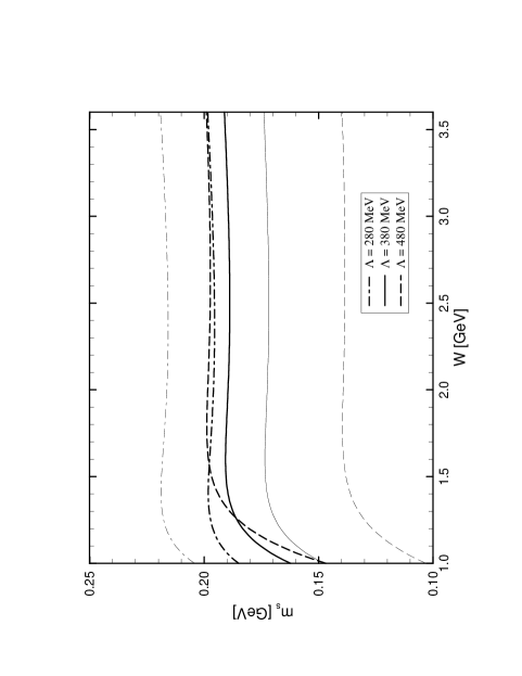
Figure 1: $m_{s}$ and $\hat{m}_{s}$ for three different values of $\Lambda_{\overline{MS}}$. Thick lines correspond to $m_{s}$ and thin lines to $\hat{m}_{s}$.

In our numerical analysis of the sum rules, we shall mainly discuss the values of our input parameters, their errors, and the impact of those errors on the strange quark mass obtained. In the OPE, we generically have to evaluate expressions of the type $\bar{a}^{m}(u)\overline{M}^{\,n}(u)$, where $m$ and $n$ are integer exponents. To achieve a systematic expansion in perturbation theory, we have decided to expand these terms consistently in inverse powers of $L\equiv\ln(u/\Lambda_{\overline{MS}}^{2})$. The relevant formula is given in eq. (B.10) in appendix B. Besides the QCD scale parameter $\Lambda_{\overline{MS}}$, it involves the RG invariant quark mass $\hat{M}$. However, as our analysis shows, the value for $\hat{m}_{s}$ depends strongly on $\Lambda_{\overline{MS}}$: it is roughly proportional to the leading term $L$. We therefore present our main results in terms of $m_{s}\equiv\overline{m}_{s}(1\,\mbox{\rm GeV})$, which only displays a mild dependence on $\Lambda_{\overline{MS}}$. In fig. 1, we show $m_{s}$ and $\hat{m}_{s}$ as calculated from the sum rule of eq. (1.9) for $\Lambda_{\overline{MS}}=280$, $380$ and $480\,\mbox{\rm MeV}$. The thick lines correspond to $m_{s}$ and the thin lines to $\hat{m}_{s}$. Our $\Lambda_{\overline{MS}}$ corresponds to 3 flavours and to NNLO, and has been chosen such that $\alpha_{s}(M_{Z})=0.118\pm 0.006$, which covers most values obtained from recent analyses [39]. All other parameters have been set to central values which will be discussed in the following.

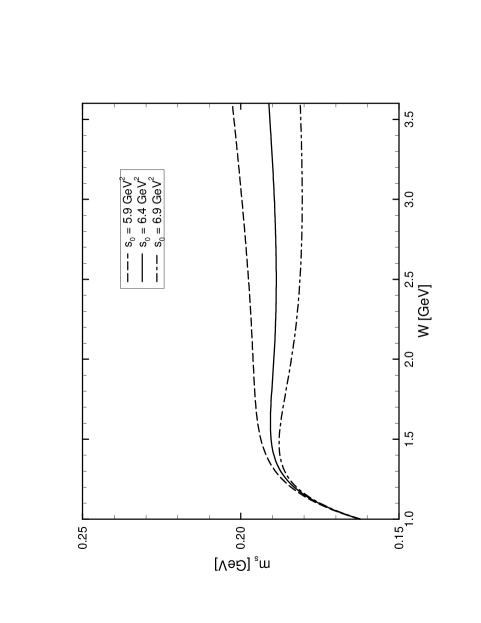
Figure 2: $m_{s}$ for three different values of $s_{0}$ and $\Lambda_{\overline{MS}}=380\,\mbox{\rm MeV}$.

Choosing the stability region from which we determine $m_{s}$ to be in the range $W\equiv\sqrt{u}=2.0$ – $3.0\,\mbox{\rm GeV}$, from fig. 1 we obtain $m_{s}=196$, 189 and $198\,\mbox{\rm MeV}$ for $\Lambda_{\overline{MS}}=280$, $380$ and $480\,\mbox{\rm MeV}$. The lower end of the stability interval has been chosen such that the ${\cal O}(a)$ correction is $~{}{}_{\textstyle\sim}^{\textstyle<}~{}50\%$ of the leading term, and at the upper end, the sum rule becomes insensitive to the hadronic resonance structure and is completely determined by the perturbative continuum. The parameter $s_{0}$ which determines the onset of the perturbative continuum has been adjusted so as to obtain optimal stability. For the three values of $\Lambda_{\overline{MS}}$ we find $s_{0}=5.5$, 6.4 and $7.5\,\mbox{\rm GeV}^{2}$ respectively. It is gratifying that $\sqrt{s_{0}}=2.5\pm 0.2\,\mbox{\rm GeV}$ is just found to be around the energy at which the next resonance, which has not been included, is expected. However, because of the imperfection of our phenomenological model, we still have a residual dependence on $s_{0}$. This dependence is displayed in fig. 2, where we plot $m_{s}$ for $\Lambda_{\overline{MS}}=380\,\mbox{\rm MeV}$ and $s_{0}=5.9$, 6.4 and $6.9\,\mbox{\rm GeV}^{2}$. We do not include this variation in the error on $m_{s}$ because it is implicitly covered through varying all other input parameters to be discussed below.

Let us next discuss the determination of the parameters in the phenomenological two-point function which has been presented in sect. 3.1. We have calculated these parameters from the experimental data for $K\pi$-scattering given by Estabrooks et al. [37] and Aston et al. [35, 36]. Generally, the s-wave amplitude and phase shift $a_{S}$ and $\phi_{S}$ can be decomposed as follows:

$$a_{S}\,e^{i\phi_{S}}\;=\;\frac{1}{2i}\,\biggl{(}\,\eta_{1}e^{2i\delta_{1}}-1\,\biggr{)}+\frac{1}{4i}\,\biggl{(}\,\eta_{3}e^{2i\delta_{3}}-1\,\biggr{)}\,,$$ (5.1)

where $\eta_{1,3}$ and $\delta_{1,3}$ are the elasticities and phase shifts for the $I=1/2$ and $I=3/2$ channel respectively. In writing eq. (5.1) we have adopted the normalisation of refs. [35, 36, 37] for $a_{S}$. In ref. [37], $\delta_{1}$ has been measured for $\sqrt{s}=0.73$ – $1.30\,\mbox{\rm GeV}$, and $\delta_{3}$ for $0.73$ – $1.72\,\mbox{\rm GeV}$. In this work it was also demonstrated that below $1.3\,\mbox{\rm GeV}$, the scattering is purely elastic, that is, $\eta_{1}=\eta_{3}=1$. On the other hand in ref. [36] only $a_{S}$ and $\phi_{S}$ up to $\sqrt{s}=2.52\,\mbox{\rm GeV}$ were given. In order to be able to calculate $\delta_{1}$ from the data by Aston et al. above $1.3\,\mbox{\rm GeV}$, we have to subtract the $I=3/2$ contribution. We fitted this contribution to a pure effective range

$$\tan\delta_{3}(s)\;=\;\alpha q(s)\Big{[}\,1+\beta q(s)^{2}\,\Big{]}\,,$$ (5.2)

where $q(s)$ is the centre of mass momentum defined in eq. (3.8). For the fit we used the full data set of ref. [37], however multiplying their error by a factor of 2 to get a $\chi^{2}/$d.o.f. of order 1, and, below $1.3\,\mbox{\rm GeV}$, for the data of ref. [36] we calculated $\delta_{3}$ from eq. (5.1) with $\eta_{1}=\eta_{3}=1$. Our best fit is obtained for: $\alpha=-1.04\,\mbox{\rm GeV}^{-1}$ and $\beta=-0.67\,\mbox{\rm GeV}^{-2}$. The value for $\alpha$ corresponds to a scattering length of $-0.20\,fm$.

Using this fit, we have then calculated $\delta_{1}$ for the data of both groups below $1.7\,\mbox{\rm GeV}$. The result obtained for $\delta_{1}$ can be fitted to the sum of an effective range and a Breit-Wigner resonance:

$$\delta_{1}(s)\;=\;\delta_{ER}(s)+\delta_{BW}(s)\,,$$ (5.3)

where $\delta_{ER}$ is again of the form given in (5.2), and

$$\tan\delta_{BW}(s)\;=\;\frac{M_{R}\Gamma_{R}(s)}{(M_{R}^{2}-s)}\,.$$ (5.4)

$\Gamma_{R}(s)$ has been defined in eq. (3.8). The lowest lying resonance in this channel is the $K_{0}^{*}(1430)$, and for our best fit we obtain: $M_{K_{0}^{*}(1430)}=1423\pm 10\,\mbox{\rm MeV}$, $\Gamma_{K_{0}^{*}(1430)}=268\pm 25\,\mbox{\rm MeV}$, $\alpha=2.06\,\mbox{\rm GeV}^{-1}$ and $\beta=-1.37\,\mbox{\rm GeV}^{-2}$. In this case $\alpha$ corresponds to a scattering length of $0.41\,fm$. $M_{K_{0}^{*}(1430)}$ and $\Gamma_{K_{0}^{*}(1430)}$ are in good agreement to the values given in [35]. We show our fit in fig. 3 together with the data points and a fit to a pure effective range below $1.3\,\mbox{\rm GeV}$. We do not give errors for $\alpha$ and $\beta$ explicitly, because they are not direct input parameters, but we have varied them for the calculation of $d(s_{+})$. We have also compared our fit to $\delta_{1}$ with other approaches, namely the $k$-matrix formalism [40], chiral perturbation theory [41, 42] and the quark Born diagram formalism [43], finding good agreement. However, the $\chi^{2}$ for our effective range plus Breit-Wigner Ansatz is lowest.

Above $1.7\,\mbox{\rm GeV}$, we do not know how to subtract the $I=3/2$ contribution. We therefore assume two extreme cases for our evaluation of the errors on $d(s_{+})$. As a lower bound for $\delta_{1}$, we use the pure effective range also displayed in fig. 3 up to infinity, and as an upper bound, above $1.7\,\mbox{\rm GeV}$ we take $\delta_{1}=180^{\circ}$ constant [8]. Using eq. (3.9) with

$$d(0)\;=\;(M_{K}^{2}-M_{\pi}^{2})\,f_{+}(0)\;=\;0.22\,\mbox{\rm GeV}^{2}\,,$$ (5.5)

and varying $\alpha$ and $\beta$ within the 1 $\sigma$ level, we find

$$d(s_{+})\;=\;0.33\pm 0.02\,\mbox{\rm GeV}^{2}\,.$$ (5.6)

This value can be compared with other methods to calculate $d(s_{+})$. Close to $s=0$, $d(s)$ can be approximated by a linear function,

$$d(s)\;=\;d(0)\,\Big{(}\,1+\lambda_{0}\,\frac{s}{M_{\pi}^{2}}\,\Big{)}\,.$$ (5.7)

Using $\lambda_{0}=0.019$ [44, 45], we get $d(s_{+})=0.31\,\mbox{\rm GeV}^{2}$. However, we know that $d(s)$ is a concave function of $s$ [45]. Thus the latter value should lie on the low side of the true value for $d(s_{+})$. On the other hand, calculating $d(s_{+})$ from chiral perturbation theory [45], we obtain $d(s_{+})=0.35\,\mbox{\rm GeV}^{2}$, also within the errors of our determination from experiment. Nevertheless, improved data for low energy $K\pi$-scattering would be of great help for a more precise determination of the hadronic parameters.

For the mass and the width of the second resonance $K_{0}^{*}(1950)$ we use the values found by Aston et al.: $M_{K_{0}^{*}(1950)}=1945\pm 22\,\mbox{\rm MeV}$ and $\Gamma_{K_{0}^{*}(1950)}=201\pm 86\,\mbox{\rm MeV}$. In addition, we need the ratio of the decay constants for the first and second resonance which determines their relative strength. From the dual-model vertex function, one finds the following parametrisation [10],

$$\frac{F_{2}}{F_{1}}\;=\;-\,\gamma\,\frac{M_{1}^{2}}{M_{2}^{2}}\,.$$ (5.8)

In our analysis we shall use $\gamma=0.5\pm 0.3$. The lower value means almost no contribution of the second resonance, whereas for the upper value, the second resonance is nearly as strong as the first one. Both being extreme cases, we think that the above range for $\gamma$ is a conservative one. The induced uncertainty on $m_{s}$ from this parameter then turns out to be $\pm\,6\,\mbox{\rm MeV}$.

Taken together, the errors in all phenomenological parameters lead to an uncertainty in the strange quark mass of $\pm\,17\,\mbox{\rm MeV}$, where we have added the errors quadratically. The dominant uncertainties in this set of parameters are due to $d(s_{+})$ and $\Gamma_{K_{0}^{*}(1430)}$, namely $\pm\,12\,\mbox{\rm MeV}$ and $\pm\,9\,\mbox{\rm MeV}$ respectively. A detailed table containing the relevant parameters entering the sum rule, their errors, and the resulting uncertainty in $m_{s}$ can be found in appendix D.

For the theoretical part of the sum rule, we still have to discuss explicit quark mass corrections, the non-perturbative condensate parameters and the ${\cal O}(a^{3})$ correction. As it turns out, because we work at a relatively high scale ($2.0$ – $3.0\,\mbox{\rm GeV}$), the quark mass and condensate contributions — except, of course, for the global quark mass factor — to the scalar sum rule are negligible. For completeness we nevertheless present our input parameters. For the light quark masses, we adopted the Particle Data values, $m_{u}\equiv\overline{m}_{u}(1\,\mbox{\rm GeV})=5\,\mbox{\rm MeV}$ and $m_{d}\equiv\overline{m}_{d}(1\,\mbox{\rm GeV})=9\,\mbox{\rm MeV}$ [46]. For the quark condensates we assume SU(3) flavour symmetry, because anyhow their contribution is tiny, and take a standard value

$$\langle\bar{q}q\rangle(1\,\mbox{\rm GeV})\;=\;-\,(225\pm 25\,\mbox{\rm MeV})^{3}\,,$$ (5.9)

where $q=u,\,d,\,s$. Let us, nevertheless, remark on the flavour dependence of the quark condensate. Because we use non-normal-ordered condensates, the strange condensate $\langle\bar{s}s\rangle$ is closer to the light quark condensate $\langle\bar{q}q\rangle$ than had we used normal-ordered condensates. Using eq. (C.1), we find $\big{<}\!\!:\!\!\bar{s}s\!\!:\!\!\big{>}/\langle\bar{s}s\rangle\approx 0.88$. Together with the known value of the flavour breaking for the normal-ordered condensate [3, 47, 48] this leads to $\langle\bar{s}s\rangle\approx 0.7\langle\bar{q}q\rangle$.

For the gluon condensate we use an average over most recent determinations, however with a quite conservative error,

$$\big{<}aFF\big{>}\;=\;0.024\pm 0.012\,\mbox{\rm GeV}^{4}\,.$$ (5.10)

This value corresponds to 1 – 3 times the standard SVZ value [1]. Finally, for the mixed condensate we take [49]

$$\langle g\bar{q}\sigma Fq\rangle\;=\;M_{0}^{2}\,\langle\bar{q}q\rangle\qquad\hbox{with}\qquad M_{0}^{2}\;=\;0.8\pm 0.2\,\mbox{\rm GeV}^{2}\,.$$ (5.11)

Again for the mixed condensate we can study its flavour dependence. Using the RG invariant combination of dimension 5 [34, 22], we find $\big{<}\!\!:\!\!g\bar{s}\sigma Fs\!\!:\!\!\big{>}/\langle g\bar{s}\sigma Fs\rangle\approx 0.99$. Therefore, the flavour breaking for the normal- and non-normal-ordered mixed condensates are almost equal. Using the values of refs. [49, 50], we thus have $\langle g\bar{s}\sigma Fs\rangle\approx 0.75\langle g\bar{q}\sigma Fq\rangle$.

The last uncertainty which we have to discuss, and unfortunately the dominant one, stems from the ${\cal O}(a^{3})$ correction. At $W=2.5\,\mbox{\rm GeV}$ and $\Lambda_{\overline{MS}}=380\,\mbox{\rm MeV}$, the ${\cal O}(a)$ correction amounts to $\approx 40\%$ and the ${\cal O}(a^{2})$ correction to $\approx 30\%$ of the leading term. Because the perturbative expansion has only asymptotic character, we conclude that the uncertainty coming from the as yet unknown ${\cal O}(a^{3})$ correction could be as large as 30%. In turn this would correspond to $c_{31}\approx 580$ if the correction is positive. For the error on $m_{s}$ we then find $\pm\,27\,\mbox{\rm MeV}$. This uncertainty turns out to be approximately halve of the error on the ${\cal O}(a^{3})$ correction, because the sum rule scales like $m_{s}^{2}$. Let us again emphasise that this is not completely consistent, because $\beta_{4}$ and $\gamma_{4}$ are unknown too, and hence have not been included. From all of the above, our main result for $m_{s}$ from the scalar sum rule is:

$$m_{s}\;=\;\overline{m}_{s}(1\,\mbox{\rm GeV})\;=\;189\pm 32\,\mbox{\rm MeV}\,.$$ (5.12)

We shall, however, try to get some idea about the ${\cal O}(a^{3})$ correction. From eq. (2.8) it is seen that the first 3 coefficients in the perturbative expansion grow almost geometrically. If this geometric growth continues for the ${\cal O}(a^{3})$ term, we would find $c_{31}\approx 440$. This would correspond to a negative 5% correction, leading to $m_{s}=178\pm 18\,\mbox{\rm MeV}$ if the phenomenological error is included.

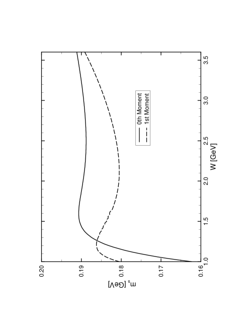
Figure 4: Comparison of $m_{s}$ from the 0th and 1st-moment sum rules.

So far, we only dealt with the sum rule of eq. (1.9). Let us now briefly analyse the 1st moment sum rule  (1.10). In fig. 4, we show the 1st moment sum rule for $\Lambda_{\overline{MS}}=380\,\mbox{\rm MeV}$ and $s_{0}=5.4\,\mbox{\rm GeV}^{2}$ in comparison to the 0th moment sum rule at $s_{0}=6.4\,\mbox{\rm GeV}^{2}$. All other parameters take their central values. It is obvious that the 1st moment sum rule is less stable. This is due to the fact that, because of the additional factor $s$ in the dispersion integral, higher states are less suppressed and the sum rule becomes more sensitive to these corrections. Within the errors the value of $m_{s}$ thus obtained agrees with our previous result. Because the 1st moment sum rule is less stable, we refrain from taking an average with the value of eq. (5.12), but we take it as a corroboration of this result.

5.2 Pseudoscalar two-point function

The hadronic input parameters for the higher resonances in the pseudoscalar channel are less well established than in the scalar channel. There are indications for two resonances with the same quantum numbers as the $K$-meson, the $K(1460)$ and the $K(1830)$ [46]. The reported widths are $\Gamma_{K(1460)}=\Gamma_{K(1830)}\approx 250\,\mbox{\rm MeV}$, although the error is probably large. Since we shall show in the following that anyhow the pseudoscalar sum rule at present should be abandoned, we just use the central values. The ratio of the decay constants of the two resonances is again given by eq. (5.8) taking $\gamma=0.5$.

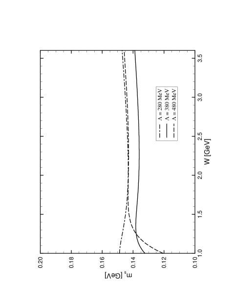
Figure 5: $m_{s}$ calculated from the pseudoscalar sum rule.

For the input parameters on the theoretical side of the sum rule, we use the same set of values as for the scalar sum rule in the previous section. In fig. 5, we display $m_{s}$ calculated from the pseudoscalar sum rule for $\Lambda_{\overline{MS}}=280$, $380$ and $480\,\mbox{\rm MeV}$. The values for $m_{s}$, obtained from this figure are $144\,\mbox{\rm MeV}$, $136\,\mbox{\rm MeV}$ and $143\,\mbox{\rm MeV}$ for $s_{0}=4.9\,\mbox{\rm GeV}$, $5.9\,\mbox{\rm GeV}$ and $6.9\,\mbox{\rm GeV}$, and the three values of $\Lambda_{\overline{MS}}$, respectively. Even though the errors on the ${\cal O}(a^{3})$ correction are large, we would expect that the central values for $m_{s}$ from scalar and pseudoscalar sum rules agree within the errors of the hadronic parametrisation, since the radiative corrections for flavour non-singlet scalar and pseudoscalar two-point functions are the same. This is, however, not the case. Let us comment on the origin of this discrepancy.

Because we evaluate the sum rule at a rather high scale, 2 – $3\,\mbox{\rm GeV}$, the dominant hadronic contribution comes from the $K(1430)$. Therefore, the error on the global coefficient of this resonance determines the largest error from the hadronic spectral function. In the case of the scalar sum rule, the corresponding quantity was the scalar form factor at threshold, $d(s_{+})$. Had we used instead the leading order chiral perturbation theory result, $d(s_{+})=d(0)=0.22\,\mbox{\rm GeV}^{2}$, the central value of $m_{s}$ would have been $127\,\mbox{\rm MeV}$ — $m_{s}$ scales linearly with $d(s_{+})$! The corrections from NLO chiral perturbation theory were large and led to $d(s_{+})=0.35\,\mbox{\rm GeV}^{2}$, quite close to the value determined from experiment.

For the pseudoscalar spectral function, we neither have available a NLO chiral perturbation theory calculation of the $(K\pi\pi)$-contribution, nor is there enough data in this system to calculate the corresponding pseudoscalar form factor from experiment. Nevertheless, an additional hint that the higher order corrections are large comes from a NLO chiral perturbation theory calculation of the matrix elements in $K_{l4}$-decays [51], which are related to the matrix elements of eqs. (3.10) and (3.11). We shall return to a calculation of the pseudoscalar spectral function at NLO chiral perturbation theory in a forthcoming publication.

A different possible parametrisation of the pseudoscalar spectral function is the zero-width approximation also for the higher resonances,

$$\rho_{5}(s)\;=\;F_{K}^{2}M_{K}^{4}\,\biggl{\{}\,\delta(s-M_{K}^{2})+r_{K}\delta(s-M_{K}^{\prime 2})+r_{K}\gamma^{2}\delta(s-M_{K}^{\prime\prime 2})\,\biggr{\}}\,,$$ (5.13)

where

$$r_{K}\;\equiv\;\frac{F_{K^{\prime}}^{2}M_{K^{\prime}}^{4}}{F_{K}^{2}M_{K}^{4}}\;=\;7\pm 1$$ (5.14)

was also determined from a sum rule analysis [3]. Here we adopted the abbreviations $K^{\prime}\equiv K(1460)$ and $K^{\prime\prime}\equiv K(1830)$. If we insert this parametrisation of the spectral function into the sum rule of eq. (1.9), we find as a central value $m_{s}=162\,\mbox{\rm MeV}$, on the low side of the strange mass region as calculated from the scalar sum rule. Let us point out, however, that the zero-width approximation only serves as a lower bound on the spectral function, and the corrections are expected to be of the order of 10 – 20% [10]. In addition, it is unclear whether the error on $r_{K}$ given in eq. (5.14) is a conservative one.

To conclude, due to unknown uncertainties in the hadronic parametrisation of the pseudoscalar spectral function, at present, we shall not use the analysis as an independent determination of $m_{s}$, but we plan to return to this issue in a future publication.

6 Discussion

Before we summarise our main results, let us discuss a few previous determinations of $m_{s}$ which are of interest in view of the present analysis.

In 1982, Gasser and Leutwyler [6] reviewed the status of quark mass determinations known at that time. For the determination of $m_{s}$, they used a combination of different QCD sum rules, together with quark mass ratios from chiral perturbation theory. Their final quoted value was $m_{s}=180\pm 50\,\mbox{\rm MeV}$. A calculation using finite energy sum rules at NNLO for scalar and pseudoscalar two-point functions was performed by Gorishny et al. [9]. For the hadronic parametrisation of the two-point functions they assumed the zero-width approximation and found $m_{s}=195\,\mbox{\rm MeV}$, where the error was estimated to be of the order of 25%.

The hadronic parametrisation of the two-point function in the scalar channel was improved in refs. [8, 10, 12] by taking resonances with a finite width. Whereas the authors of [8] only gave a lower bound on the strange quark mass, the final result of ref. [12] was $m_{s}=192\pm 15\,\mbox{\rm MeV}$. Since this was only a NLO calculation, due to the large radiative corrections, the error in this determination appears to be too small. In ref. [13], Dominguez and de Rafael determined the strange mass by first calculating $m_{u}+m_{d}$ from the pseudoscalar sum rule for light quarks and then applying quark mass ratios from chiral perturbation theory to find $m_{s}=199\pm 33\,\mbox{\rm MeV}$. They also refrained from using the pseudoscalar sum rule for the $K$-channel directly because of large uncertainties in the hadronic parametrisation. Although it is not obvious that the parametrisation of the spectral function is more reliable in the case of light quarks $m_{u}$ and $m_{d}$, their central value is in good agreement to our results. The work of Narison is summarised in refs. [3, 17]. By purely analysing the pseudoscalar channel, he obtained $m_{s}=169\pm 10\,\mbox{\rm MeV}$, whereas his final result for an average over determinations from different sum-rule channels gave $m_{s}=160\pm 9\,\mbox{\rm MeV}$. The further reduction of $m_{s}$ is caused by the rather low value found in the $\phi\,$-meson channel, although the errors are very large.

The last sum-rule determination which we would like to discuss, and the one which comes closest to our analysis of the scalar channel, is the work by Dominguez et al. [19]. The main differences are the following: they only used NLO expressions for the perturbative two-point function, they did not include the cancellation of mass singularities for the gluon condensate and the hadronic spectral function had been parametrised differently. Nevertheless, their final result, $m_{s}=194\pm 4\,\mbox{\rm MeV}$, is in good agreement to our findings. However, the quoted error was obtained by varying solely $\Lambda_{\overline{MS}}$. Since this is a minor source of uncertainty, to our minds, their error is largely underestimated. Very recently, the strange quark mass was calculated from lattice QCD [52]. The result was $\overline{m}_{s}(2\,\mbox{\rm GeV})=127\pm 18\,\mbox{\rm MeV}$. Scaling this value down to $\mu=1\,\mbox{\rm GeV}$, we find $m_{s}=180\pm 25\,\mbox{\rm MeV}$.

All determinations of the strange quark mass from QCD sum rules which have been discussed above are in general agreement with the calculation presented in this work, although in some analyses the errors were underestimated. Our main result was obtained from a sum rule for the divergence of the vector current: $m_{s}=189\pm 32\,\mbox{\rm MeV}$. In this determination, the error is dominated by the unknown perturbative ${\cal O}(a^{3})$ correction. We tried to estimate the ${\cal O}(a^{3})$ correction by observing a geometric growth of the first three terms in the perturbation series, and assuming that this geometric behaviour continues for the next order. The result then is: $m_{s}=178\pm 18\,\mbox{\rm MeV}$, where the error now dominantly stems from the hadronic parametrisation of the spectral function. Especially this latter value is in astonishing agreement with the lattice calculation of ref. [52]. The sum rule for the divergence of the axial-vector was found to be unreliable, due to large uncertainties in the hadronic parametrisation of the spectral function. Recently, instanton contributions to the determination of light quark masses were investigated [53], and it was found that they can be sizeable if the scale at which the sum rule is evaluated, is too low. Because of the relatively large scale at which we obtain the strange mass, in the case at hand these contributions can be safely neglected.

As a final application of our results, we estimate the masses of the light quarks $m_{u}$ and $m_{d}$ from quark-mass ratios calculated in chiral perturbation theory, and the mass of the strange quark obtained in the present work. The relevant quark-mass ratios are [54, 45]

$$\frac{2m_{s}}{m_{u}+m_{d}}\;=\;25.7\pm 2.6\qquad\mbox{and}\qquad\frac{m_{d}-m_{u}}{m_{u}+m_{d}}\;=\;0.28\pm 0.03\,.$$ (6.1)

Using $m_{s}=189\pm 32\,\mbox{\rm MeV}$, we find $m_{u}=5.3\pm 1.5\,\mbox{\rm MeV}$ and $m_{d}=9.4\pm 1.5\,\mbox{\rm MeV}$, whereas for $m_{s}=178\pm 18\,\mbox{\rm MeV}$ we obtain $m_{u}=5.0\pm 1.1\,\mbox{\rm MeV}$ as well as $m_{d}=8.9\pm 1.1\,\mbox{\rm MeV}$, in good agreement to earlier determinations published in the literature. We plan to directly investigate quark-mass ratios from QCD sum rules in the future.

Acknowledgement

It is a pleasure to thank A. J. Buras, H. G. Dosch and A. Pich for helpful discussions. M. J. would also like to thank T. Barnes and E. de Rafael for e-mail discussions, C. Ayala and J. R. Peláez for providing Fortran programs related to their work and D. Pirjol for making available a preliminary version of a paper on the same subject, prior to publication.

Appendices

Appendix A The Borel transform

The Borel operator ${\cal B}$ is defined by ($s\equiv Q^{2}$)

$${\cal B}_{u}\;\equiv\;\lim_{\stackrel{{\scriptstyle s,n\to\infty}}{{s/n=u}}}\frac{(-s)^{n}}{(n-1)!}\,\frac{\partial^{\,n}}{(\partial s)^{n}}\,.$$ (A.1)

The Borel transformation is an inverse Laplace transform [55]. If we set

$$\widehat{f}(u)\;\equiv\;{\cal B}_{u}\Big{[}\,f(s)\,\Big{]}\,,\qquad\hbox{then}\qquad f(s)\;=\;\int\limits_{0}^{\infty}\frac{1}{u}\,\widehat{f}(u)\,e^{-s/u}du\,.$$ (A.2)

We need the following Borel transforms [56]:

$${\cal B}_{u}\biggl{[}\,\frac{1}{s^{\alpha}}\,\ln^{n}\frac{s}{\mu^{2}}\,\biggr{]}\;=\;\frac{1}{u^{\alpha}}\sum_{k=0}^{n}(-)^{n-k}{n\choose k}\ln^{k}\frac{u}{\mu^{2}}\,\Biggl{[}\,\frac{\partial^{\,n-k}}{(\partial\alpha)^{n-k}}\,\frac{1}{\Gamma(\alpha)}\,\Biggr{]}\,,$$ (A.3)

and explicitly for $n=0,\,1,\,2,\,3$:

$${\cal B}_{u}\biggl{[}\,\frac{1}{s^{\alpha}}\,\biggr{]} = \frac{1}{u^{\alpha}\Gamma(\alpha)}\,,$$

$$\vbox{\vskip 22.76219pt}{\cal B}_{u}\biggl{[}\,\frac{1}{s^{\alpha}}\,\ln\frac{s}{\mu^{2}}\,\biggr{]} = \frac{1}{u^{\alpha}\Gamma(\alpha)}\,\Big{[}\,\bar{L}+\psi(\alpha)\,\Big{]}\,,$$ (A.4)

$$\vbox{\vskip 22.76219pt}{\cal B}_{u}\biggl{[}\,\frac{1}{s^{\alpha}}\,\ln^{2}\frac{s}{\mu^{2}}\,\biggr{]} = \frac{1}{u^{\alpha}\Gamma(\alpha)}\,\Big{[}\,\bar{L}^{2}+2\psi(\alpha)\bar{L}+\psi^{2}(\alpha)-\psi^{\prime}(\alpha)\,\Big{]}\,,$$

$$\vbox{\vskip 22.76219pt}{\cal B}_{u}\biggl{[}\,\frac{1}{s^{\alpha}}\,\ln^{3}\frac{s}{\mu^{2}}\,\biggr{]} = \frac{1}{u^{\alpha}\Gamma(\alpha)}\,\Big{[}\,\bar{L}^{3}+3\psi(\alpha)\bar{L}^{2}+3\big{(}\psi^{2}(\alpha)-\psi^{\prime}(\alpha)\big{)}\bar{L}+\psi^{3}(\alpha)$$

$$\hskip 62.59605pt-\,3\psi(\alpha)\psi^{\prime}(\alpha)+\psi^{\prime\prime}(\alpha)\,\Big{]}\,.$$

Here, $\bar{L}\equiv\ln u/\mu^{2}$ and

$$\psi^{(k)}(\alpha)\;\equiv\;\frac{\partial^{\,k+1}}{(\partial\alpha)^{k+1}}\,\ln\Gamma(\alpha)\,.$$ (A.5)

For integer values of $\alpha$, we have the following useful formulae [38]:

$$\psi(n) = \sum_{l=1}^{n-1}\frac{1}{l}-\gamma_{E}\,,$$

$$\vbox{\vskip 22.76219pt}\psi^{(k)}(n) = (-)^{k}\,k!\,\Biggl{[}\,\sum_{l=1}^{n-1}\frac{1}{l^{k+1}}-\zeta(k+1)\,\Biggr{]}\,;\qquad k\geq 1\,.$$ (A.6)

To arrive at eq. (1.6), we also need:

$${\cal B}_{u}\biggl{[}\,\frac{1}{(x+s)^{\alpha}}\,\biggr{]}\;=\;\frac{1}{u^{\alpha}\Gamma(\alpha)}\,e^{-x/u}\,.$$ (A.7)

Appendix B Renormalization group functions

For the definition of the renormalization group functions we follow the notation of Pascual and Tarrach [57], except that we defined the $\beta$-function such that $\beta_{1}$ is positive. The expansions of $\beta(a)$ and $\gamma(a)$ take the form:

$$\beta(a)\;=\;-\,\beta_{1}a-\beta_{2}a^{2}-\beta_{3}a^{3}-\ldots\,,\quad\hbox{and}\quad\gamma(a)\;=\;\gamma_{1}a+\gamma_{2}a^{2}+\gamma_{3}a^{3}+\ldots\,,$$ (B.8)

with

$$\beta_{1}\;=\;\frac{1}{6}\,\Big{[}\,11N-2f\,\Big{]}\,,\qquad\beta_{2}\;=\;\frac{1}{12}\,\Big{[}\,17N^{2}-5Nf-3C_{F}f\,\Big{]}\,,\qquad\qquad{}$$ (B.9)

$$\beta_{3}\;=\;\frac{1}{32}\,\biggl{[}\,\frac{2857}{54}N^{3}-\frac{1415}{54}N^{2}f+\frac{79}{54}Nf^{2}-\frac{205}{18}NC_{F}f+\frac{11}{9}C_{F}f^{2}+C_{F}^{2}f\,\biggr{]}\,,$$

and

$$\gamma_{1}\;=\;\frac{3}{2}\,C_{F}\,,\qquad\qquad\qquad\gamma_{2}\;=\;\frac{C_{F}}{48}\,\Big{[}\,97N+9C_{F}-10f\,\Big{]}\,,\hskip 56.9055pt{}$$

$$\gamma_{3}\;=\;\frac{C_{F}}{32}\,\biggl{[}\,\frac{11413}{108}N^{2}-\frac{129}{4}NC_{F}-\Big{(}\frac{278}{27}+24\zeta(3)\Big{)}Nf+\frac{129}{2}C_{F}^{2}-\Big{(}23-24\zeta(3)\Big{)}C_{F}f-\frac{35}{27}f^{2}\,\biggr{]}\,,$$

where $\gamma_{3}$ has been taken from ref. [58].

We also need the expansion of an arbitrary product $\bar{a}^{m}(u)\overline{M}^{\,n}(u)$ in inverse powers of $L\equiv\ln(u/\Lambda^{2})$:

$$\bar{a}^{m}(u)\,\overline{M}^{\,n}(u)\;=\;\frac{\hat{M}^{n}}{\beta_{1}^{m}}\,\biggl{(}\frac{2}{L}\biggr{)}^{m+n\,\gamma_{1}/\beta_{1}}\biggr{[}\,1+d_{11}\,\frac{\ln L}{L}+\frac{d_{10}}{L}+d_{22}\,\frac{\ln^{2}L}{L^{2}}+d_{21}\;\frac{\ln L}{L^{2}}+\frac{d_{20}}{L^{2}}\,\biggr{]}\,,$$ (B.10)

with

$$d_{11} = -\,\frac{2\beta_{2}}{\beta_{1}^{3}}\,\Big{(}m\,\beta_{1}+n\,\gamma_{1}\Big{)}\,,\hskip 28.45274ptd_{10}\;=\;\frac{2n}{\beta_{1}^{3}}\,\Big{(}\beta_{1}\gamma_{2}-\beta_{2}\gamma_{1}\Big{)}\,,$$

$$d_{22} = \frac{1}{2}\,d_{11}^{2}-\frac{\beta_{2}}{\beta_{1}^{2}}\,d_{11}\,,\hskip 62.59596ptd_{21}\;=\;d_{11}d_{10}-\frac{4\beta_{2}}{\beta_{1}^{4}}\,\Big{(}m\,\beta_{2}+n\,\gamma_{2}\Big{)}\,,$$ (B.11)

$$d_{20} = \frac{1}{2}\,\Big{(}d_{21}-d_{11}d_{10}+d_{10}^{2}\Big{)}+\frac{2}{\beta_{1}^{3}}\,\Big{(}m\,\beta_{3}+n\,\gamma_{3}\Big{)}-\frac{d_{11}}{\beta_{1}^{2}\beta_{2}}\,\Big{(}\beta_{1}\beta_{3}-\beta_{2}^{2}\Big{)}\,.$$

Here, $\hat{M}$ is the renormalization group invariant quark mass. Because $\gamma_{1}/\beta_{1}$ is close to $1/2$, from the prefactor of eq. (B.10) we read off that two powers of $M$ count approximately like $a$ in the perturbative expansion. This way of counting orders in perturbation theory has been adopted in this work.

Using the renormalization group equation (2.5), we find the following relations between the $c_{ij}$:

$$c_{12} = -\,\frac{1}{2}\,\gamma_{1}c_{01}\,,$$

$$\vbox{\vskip 17.07164pt}c_{22} = -\,\frac{1}{4}\,\Big{[}\,\big{(}\beta_{1}+2\gamma_{1}\big{)}c_{11}+2\gamma_{2}c_{01}\,\Big{]}\,,$$ (B.12)

$$\vbox{\vskip 17.07164pt}c_{23} = \phantom{-}\,\frac{1}{12}\,\gamma_{1}\big{(}\beta_{1}+2\gamma_{1}\big{)}c_{01}\,,$$

$$\vbox{\vskip 22.76219pt}c_{32} = -\,\frac{1}{4}\,\Big{[}\,2\big{(}\beta_{1}+\gamma_{1}\big{)}c_{21}+\big{(}\beta_{2}+2\gamma_{2}\big{)}c_{11}+2\gamma_{3}c_{01}\,\Big{]}\,,$$

$$\vbox{\vskip 17.07164pt}c_{33} = -\,\frac{1}{6}\,\Big{[}\,(\beta_{2}+2\gamma_{2})c_{12}+2(\beta_{1}+\gamma_{1})c_{22}\,\Big{]}\,,$$ (B.13)

$$\vbox{\vskip 17.07164pt}c_{34} = -\,\frac{1}{4}\,(\beta_{1}+\gamma_{1})c_{23}\,.$$

Appendix C Renormalization group invariant condensates

To the order considered in this work the renormalization group invariant condensates are given by [34, 31]:

$$\Omega^{m_{i}q_{j}}_{3} \equiv m_{i}\langle\bar{q}_{j}q_{j}\rangle+w_{1}\,\biggl{[}\,\frac{1}{a}+w_{2}\,\biggr{]}\,m_{i}\,m_{j}^{3}\,,$$ (C.1)

$$\vbox{\vskip 22.76219pt}\Omega_{4} \equiv \langle aFF\rangle-4\,\frac{\gamma_{1}}{\beta_{1}}\,a\sum_{i}m_{i}\langle\bar{q}_{i}q_{i}\rangle-\frac{\gamma_{1}^{0}}{\beta_{1}}\sum_{i}m_{i}^{4}\,,$$ (C.2)

where

$$w_{1}\;=\;\frac{\gamma_{1}^{0}}{(4\gamma_{1}-\beta_{1})}\,,\qquad w_{2}\;=\;\frac{1}{6}\,(4\gamma_{1}-\beta_{1})-\frac{1}{4\gamma_{1}}\,(4\gamma_{2}-\beta_{2})\,,$$ (C.3)

and $\gamma_{1}^{0}=N/(2\pi^{2})$ is the leading order anomalous dimension of the vacuum energy.

Appendix D Input parameters and the error on $m_{s}$

We have omitted those input parameters from the table whose variation results in an error on $m_{s}$ less than $1\,\mbox{\rm MeV}$.

Parameter	Value	$\Delta m_{s}$
$\Lambda_{\overline{MS}}$	$380\pm 100\,\mbox{\rm MeV}$	$\pm\,5\,\mbox{\rm MeV}$
${\cal O}(a^{3})$		$\pm\,27\,\mbox{\rm MeV}$
$d(s_{+})$	$0.33\pm 0.02\,\mbox{\rm GeV}^{2}$	$\pm\,12\,\mbox{\rm MeV}$
$M_{K_{0}^{*}(1430)}$	$1423\pm 10\,\mbox{\rm MeV}$	$\pm\,3\,\mbox{\rm MeV}$
$\Gamma_{K_{0}^{*}(1430)}$	$268\pm 25\,\mbox{\rm MeV}$	$\pm\,9\,\mbox{\rm MeV}$
$\Gamma_{K_{0}^{*}(1950)}$	$201\pm 86\,\mbox{\rm MeV}$	$\pm\,4\,\mbox{\rm MeV}$
$\gamma$	$0.5\pm 0.3$	$\pm\,6\,\mbox{\rm MeV}$

Figure 3: Our fit for the $s$-wave $I=1/2$ phase shift, compared to the experimental data. The thin line corresponds to a pure effective range.

References

• [1] M. A. Shifman, A. I. Vainshtein, and V. I. Zakharov, Nucl. Phys. B147 (1979) 385, 448, 519.
• [2] L. J. Reinders, H. Rubinstein, and S. Yazaki, Phys. Rep. 127 (1985) 1.
• [3] S. Narison, QCD Spectral Sum Rules, World Scientific Lecture Notes in Physics – Vol. 26, 1989.
• [4] M. Shifman (Ed.), Vacuum Structure and QCD Sum Rules, North-Holland, 1992.
• [5] C. Becchi, S. Narison, E. de Rafael, and F. J. Ynduráin, Z. Phys. C8 (1981) 335.
• [6] J. Gasser and H. Leutwyler, Phys. Rep. C87 (1982) 77.
• [7] S. Mallik, Nucl. Phys. B206 (1982) 90.
• [8] S. Narison, N. Paver, E. de Rafael, and D. Treleani, Nucl. Phys. B212 (1983) 365.
• [9] S. G. Gorishny, A. L. Kataev, and S. A. Larin, Phys. Lett. 135B (1984) 457.
• [10] C. A. Dominguez, Z. Phys. C26 (1984) 269.
• [11] L. J. Reinders and H. R. Rubinstein, Phys. Lett. 145B (1984) 108.
• [12] C. A. Dominguez and M. Loewe, Phys. Rev. D31 (1985) 2930.
• [13] C. A. Dominguez and E. de Rafael, Ann. Phys. 174 (1987) 372.
• [14] C. Ayala, E. Bagan, and A. Bramon, Phys. Lett. 189B (1987) 347.
• [15] S. Narison, Rev. Nuov. Cim. Vol. 10 (1987) 1.
• [16] D. J. Broadhurst and S. C. Generalis, Open University Report, No.OUT-4102-12 (1984).
• [17] S. Narison, Phys. Lett. 216B (1989) 191.
• [18] S. C. Generalis, J. Phys. G 16 (1990) L117.
• [19] C. A. Dominguez, C. van Gend, and N. Paver, Phys. Lett. B253 (1991) 241.
• [20] A. J. Buras, M. Jamin, and M. E. Lautenbacher, Nucl. Phys. B408 (1993) 209.
• [21] M. Ciuchini, E. Franco, G. Martinelli, and L. Reina, Phys. Lett. B301 (1993) 263.
• [22] M. Jamin and M. Münz, Z. Phys. C60 (1993) 569.
• [23] N. N. Bogolyubov, B. V. Medvedev, and M. K. Polivanov, Theory of dispersion relations, Moscow State Technical Publishing House, 1958.
• [24] K. Wilson, Phys. Rev. 179 (1969) 1499.
• [25] W. A. Bardeen, A. J. Buras, D. W. Duke, and T. Muta, Phys. Rev. D18 (1978) 3998.
• [26] S. G. Gorishny, A. L. Kataev, S. A. Larin, and L. R. Surguladze, Mod. Phys. Lett. A5 (1990) 2703.
• [27] C. Ayala, Ann. Phys. 208 (1991) 376.
• [28] C. Ayala, Comp. Phys. Comm. 70 (1992) 401.
• [29] Y. Chung, H. G. Dosch, M. Kremer, and D. Schall, Z. Phys. C25 (1984) 151.
• [30] S. C. Generalis, J. Phys. G 16 (1990) 785.
• [31] V. P. Spiridonov and K. G. Chetyrkin, Sov. J. Nucl. Phys. 47 (1988) 522.
• [32] K. G. Chetyrkin, S. G. Gorishny, and V. P. Spiridonov, Phys. Lett. 160B (1985) 149.
• [33] P. Pascual and E. de Rafael, Z. Phys. C12 (1982) 127.
• [34] S. Narison and R. Tarrach, Phys. Lett. 125B (1983) 217.
• [35] D. Aston et al., Nucl. Phys. B296 (1988) 493.
• [36] N. Awaji, Ph.D. thesis, Nagoya University, 1986, (unpublished).
• [37] P. Estabrooks et al., Nucl. Phys. B133 (1978) 490.
• [38] I. S. Gradshteyn and I. M. Ryzhik, Tables of integrals, series, and products, Academic Press, 1980.
• [39] S. Bethke, talk presented at ‘QCD 94’, Montpellier, July 1994.
• [40] C. B. Lang and W. Porod, Phys. Rev. D21 (1980) 1295.
• [41] V. Bernard, N. Kaiser, and U. G. Meißner, Nucl. Phys B364 (1991) 283.
• [42] A. Dobado and J. R. Peláez, Phys. Rev. D47 (1993) 4883.
• [43] Z. Li, M. Guidry, T. Barnes, and E. S. Swanson, MIT preprint MIT-CTP-2277 (1994), hep-ph/9401326.
• [44] G. Donaldson et al., Phys. Rev. D9 (1974) 2960.
• [45] J. Gasser and H. Leutwyler, Nucl. Phys. B250 (1985) 465, 517.
• [46] Particle Data Group, Review of Particle Properties, Phys. Rev. D50 (1994).
• [47] Y. Chung, H. G. Dosch, M. Kremer, and D. Schall, Phys. Lett. 102B (1981) 175.
• [48] H. G. Dosch, M. Jamin, and S. Narison, Phys. Lett. B220 (1989) 251.
• [49] A. A. Ovchinnikov and A. A. Pivovarov, Sov. J. Nucl. Phys. 48 (1988) 721.
• [50] M. Beneke and H. G. Dosch, Phys. Lett. B284 (1992) 116.
• [51] J. Bijnens, G. Colangelo, and J. Gasser, $K_{l4}$-decays beyond one loop, BUTP-94/4, hep-ph/9403390, to appear in Nucl. Phys. B .
• [52] C. R. Allton et al., Quark masses from lattice QCD at the next-to-leading order, CERN-TH.7256/94, hep-ph/9406263 .
• [53] E. Gabrielli and P. Nason, Phys. Lett. B313 (1993) 430.
• [54] J. Gasser and H. Leutwyler, Ann. Phys. 158 (1984) 142.
• [55] D. V. Widder, The Laplace Transform, Princton University Press, 1946.
• [56] A. P. Prudnikov, Y. A. Brychkov, and O. I. Marichev, Integrals and Series, Vol. 5, Gordon and Breach, 1992.
• [57] P. Pascual and R. Tarrach, QCD: Renormalization for the Practitioner, Lecture Notes in Physics 194, Springer-Verlag, 1984.
• [58] O. V. Tarasov, Dubna Report No. JINR P2-82-900 (1982) (unpublished).
Refer to caption