NORDITA-94/44 N,P

revised

$B_{K}$ and Explicit Chiral Symmetry Breaking
Johan Bijnens^a and Joaquim Prades^a,b
a NORDITA, Blegdamsvej 17,

DK-2100 Copenhagen Ø, Denmark

^b Niels Bohr Institute, Blegdamsvej 17,

DK-2100 Copenhagen Ø, Denmark

The $B_{K}$ parameter is discussed in the general context of calculating beyond the factorization approximation for hadronic matrix elements. A variant of the $1/N_{c}$ method of Bardeen et al. is used. We present calculations within a low energy approach and a calculation within the Nambu–Jona-Lasinio model. Matching with the QCD behaviour and dependence on non-zero current quark masses is studied.

September 1994

1 Introduction

The problem of calculating matrix elements of weak decay operators is a rather old one. In this letter we will restrict ourselves to the matrix element between two on-shell kaon states of the following $\Delta S=2$ four-quark operator

$${\cal O}_{\Delta S=2}(x)\equiv L^{sd}_{\mu}(x)L_{sd}^{\mu}(x)$$ (1)

with $L^{sd}_{\mu}(x)=\overline{s}(x)\gamma_{\mu}\left(\frac{\displaystyle 1-\gamma_{5}}{\displaystyle 2}\right)d(x)$ and summation over colours is understood. This matrix element is usually parametrized in the form of the $B_{K}$-parameter times the vacuum insertion approximation (VIA) as follows

$${}\langle\overline{K}^{0}|{\cal O}_{\Delta S=2}(x)|K^{0}\rangle\equiv\frac{\displaystyle 4}{\displaystyle 3}B_{K}(\mu)f^{2}_{K}m_{K}^{2}$$ (2)

where $f_{K}$ denotes the $f_{K}\to\mu\nu$ coupling ($f_{K}=113$ MeV in this normalization) and $m_{K}$ is the $K^{0}$ mass. The $\mu$-scale dependence of $B_{K}$ reflects the fact that the four-quark operator ${\cal O}_{\Delta S=2}$ has an anomalous dimension and its matrix element runs between the scale where the operator has a hadronic realization and the scale where it matches the quark-gluon realization of QCD. This anomalous dimension is known and using the renomalization group leads to the definition of the scale invariant quantity

$$\hat{B}_{K} = B_{K}(\mu)\alpha_{S}(\mu)^{a_{+}}$$ (3)

with

$$a_{+}=\frac{\displaystyle 3}{\displaystyle-2\beta^{(1)}}\left(1-\frac{\displaystyle 1}{\displaystyle N_{c}}\right)$$ (4)

at one-loop. Here $\beta^{(1)}$ is the QCD beta function first coefficient. For three active quark flavours and $N_{c}=3$ we have $a_{+}=-2/9$.

The vacuum insertion approximation was historically the first way this particular matrix element was evaluated [1]. Here by definition we have $B_{K}(\mu)=1$ at any scale and we can only obtain an order of magnitude estimate. Next this matrix element was related to the $\Delta I=3/2$ part of $K\to\pi\pi$ by Donoghue et al.[2] using SU(3) symmetry and PCAC. This leads to a value $\hat{B}_{K}\approx 0.37$. It was then found that this relation has rather large corrections[3] due to SU(3) breaking. Then three new analytical approaches appeared, the hadronic duality approach [4], QCD sum rules using three-point functions[5] and the $1/N_{c}$ expansion [6]. The lattice QCD method also started producing preliminary results around this time. A review of the situation several years ago can be found in the proceedings of the Ringberg workshop devoted to this subject[7]. All these approaches have in common that they try to get a numerical value for the $B_{K}$ parameter and study its dependence on the renormalization scale $\mu$. All of these methods have been updated and refined. The hadronic duality update can be found in [8], a QCD sum rule calculation is in [9] and the $1/N_{c}$ expansion method has had the vector meson contribution calculated in a Vector Meson Dominance (VMD) model[10]. A review of recent lattice results can be found in [11]. A full Chiral Perturbation Theory (CHPT) approach to the problem is unfortunately not possible. The data on kaon nonleptonic decays do not allow to determine all relevant parameters at next-to-leading order (${\cal O}(p^{4})$) in the nonleptonic chiral Lagrangian[12]. A calculation of these parameters within a QCD inspired model can be found in [13] where the determination of the $B_{K}$ factor is done to ${\cal O}(p^{4})$.

The leading order result for $B_{K}$ in the $1/N_{c}$ expansion is well known

$${}B_{K}(\mu)=\hat{B}_{K}=\frac{\displaystyle 3}{\displaystyle 4}.$$ (5)

This result is model independent. However, to go further in the $1/N_{c}$ expansion requires some model dependent assumptions. Different low-energy models are then used in variants on the $1/N_{c}$ method[6]. An example is the calculation done within the QCD-effective action model[14]. In fact the $\pi^{+}-\pi^{0}$ mass difference has been used to test all of the different $1/N_{c}$ methods, the original one including vector mesons [15], the QCD-effective action model [16] and the extended Nambu-Jona-Lasinio (ENJL) model[17]. The advantage of the latter model is that it has been shown to give a good picture of the parameters in the chiral Lagrangian including the SU(3) breaking ones, see [18] and references therein. In fact this model accounts for a rather large body of low energy hadronic data, see [19] for a review. The reason to resort to a model of this type is that if we also would like to know possible SU(3) breaking effects, we cannot use a simple vector meson model because we need to know the SU(3) breaking of couplings of the resonances to external currents. In practice a large part of these effects comes from scalar resonances which are experimentally rather poorly known. We could then use a model to estimate these couplings but it seems to make more sense then to calculate the relevant quantity directly within the model. It is also important to know the higher order couplings beyond order $p^{4}$ since weak matrix elements involve an integration over internal momenta.

In this letter we shall give the results for the next-to-leading corrections to (5) for the simple NJL model without a vector like coupling. This does not include vector mesons so it will not be the final answer but one can already do a study of the SU(3) breaking effects since these tend to come mainly from the scalar sector. Results on the full model and more details regarding the present work will be presented elsewhere[20]. The full model requires inclusion of anomalous diagrams and involves about an order of magnitude more terms than the present work.

We will first discuss the method and then use CHPT to derive first results. This is essentially the method of [6] in a slightly different notation. This will also allow us to test at low cut-offs the calculation done afterwards. Next we describe the NJL model and give the lowest order result in $1/N_{c}$. Then we describe the main part of the work. The calculation of the non factorizable part of the $\Delta S=2$ two-point function in the NJL model. Next we discuss how the Fierz-contribution is reproduced analytically in this approach and how it affects the final result. We will give numerical results for the case of massless quarks, of non-zero degenerate quark masses and of different quark masses. In the end we present our main conclusions.

2 The method and definitions

We calculate here not directly the $B_{K}$-factor but the $\Delta S=2$ two-point function

$$G_{F}\,\Pi_{\Delta S=2}(q^{2}) \equiv i\int d^{4}x\,e^{iq\cdot x}\,e^{i\Gamma_{\Delta S=2}}\langle 0|T\left(P^{ds}(0)P^{ds}(x)\right)|0\rangle$$ (6)

$$= i^{2}\int d^{4}x\,e^{iq\cdot x}\langle 0|T\left(P^{ds}(0)P^{ds}(x)\Gamma_{\Delta S=2}\right)|0\rangle$$

in the presence of strong interactions. We shall use the NJL model for scales below or around the spontaneous symmetry breaking scale. Here $G_{F}$ is the Fermi coupling constant, we use $P^{ds}(x)=\overline{d}(x)i\gamma_{5}s(x)$, with summation over colour understood and

$${}\Gamma_{\Delta S=2}=-G_{F}\,\int d^{4}y\,{\cal O}_{\Delta S=2}(y).$$ (7)

The reason to calculate this two-point function rather than directly the matrix element is that we can now perform the calculation fully in the Euclidean region so we do not have the problem of imaginary scalar products. This also allows us in principle to obtain an estimate of off-shell effects in the matrix elements. This will be important in later work to assess the uncertainty when trying to extrapolate from $K\to\pi$ decays to $K\to 2\pi$. This quantity is also very similar to what is used in the lattice and QCD sum rule calculations of $B_{K}$.

The $\Delta S=2$ operator in (7) can be rewritten as

$${}\Gamma_{\Delta S=2} = -G_{F}\,\int d^{4}yL^{sd}_{\mu}(y)L_{sd}^{\mu}(y)$$ (8)

$$= -G_{F}\,\int\frac{d^{4}r}{(2\pi)^{4}}\int d^{4}x_{1}\int d^{4}x_{2}\,e^{-ir\cdot(x_{2}-x_{1})}L^{sd}_{\mu}(x_{1})L_{sd}^{\mu}(x_{2}).$$

This allows us to consider this operator as being produced at the $M_{W}$ scale by the exchange of a heavy $X$ $\Delta S=2$ boson. We will work in the Euclidean domain where all momenta squared are negative. The integral in the modulus of the momentum $r$ in (8) is then split into two parts,

$$\int_{0}^{M_{W}}d|r|=\int_{0}^{\mu}d|r|+\int_{\mu}^{M_{W}}d|r|\ .$$ (9)

In principle one should then evaluate both parts separately as was done for the $\pi^{+}-\pi^{0}$ mass difference in the above quoted references. Here we will do the upper part of the integral using the renormalization group. This results in the integral being of the same form but multiplied with the Wilson coefficient $C(\mu)$,

$${}\Gamma_{\Delta S=2}=-G_{F}\,C(\mu)\int_{0}^{\mu}\frac{d^{4}r}{(2\pi)^{4}}\int d^{4}x_{1}\int d^{4}x_{2}\,e^{-ir\cdot(x_{2}-x_{1})}L^{sd}_{\mu}(x_{1})L_{sd}^{\mu}(x_{2})$$ (10)

A strict analysis in $1/N_{c}$ would correspond to set $C(\mu)=1+d(\mu)\alpha_{S}(\mu)$ and to evaluate the second term using factorization in leading $1/N_{c}$. $d(\mu)$ is what the one-gluon exchange diagrams would give with a lower cut-off $\mu$. We will however use the full one-loop Wilson coefficient $C(\mu)=\left(\alpha_{S}(\mu)/\alpha_{S}(M_{W})\right)^{a_{+}}$. In the remainder formulas this factor will be suppressed for simplicity. The lower part of the integral is then evaluated using the NJL model.

To illustrate the procedure let us calculate the relevant quantities in chiral perturbation theory. This will only make sense for a scale $\mu$ such that CHPT can be trusted. The lowest order (LO) contribution comes from the diagram in fig. 1a.

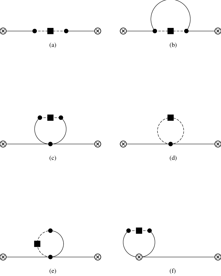
Figure 1: Chiral Perturbation Theory contributions to $\Pi_{\Delta S=2}(q^{2})$. (a) Lowest order. (b-f) Higher order non-factorizable. A circled cross is an insertion of the external pseudoscalar current, $P^{sd}(x)$, a dot is a strong interaction vertex and the square represents the $\Delta S=2$ operator, $\Gamma_{\Delta S=2}$. The full lines are meson lines.

The vertices at this order can be obtained from the standard chiral Lagrangian of order $p^{2}$. The result is

$${}\Pi_{\Delta S=2}(q^{2})_{CHPT-LO}=-2B_{0}^{2}F_{0}^{4}\frac{q^{2}}{\left(q^{2}-m_{K}^{2}\right)^{2}}\ .$$ (11)

The parameter $B_{0}$ is related to the quark condensate in the chiral limit by $\langle\overline{q}q\rangle=-B_{0}F_{0}^{2}$ and $F_{0}$ is the pion decay constant in the chiral limit, $F_{0}\approx 86$ MeV. At this order, the only nonvanishing contributions are leading in $1/N_{c}$, therefore when the result in (11) is properly reduced (see [21]) and compared with eq. (2) one gets the leading order $1/N_{c}$ result in eq. (5).

At next-to-leading order (NLO) in the chiral expansion more diagrams have to be taken into account. The ones that are non-factorizable (NF), i.e., the ones that are not reducible when the $X$ boson propagator gets cut, are depicted in fig. 1b-f (plus the last one symmetrized). Here the vector-vector part of the interaction contributes in diagrams b and d while the axial-axial part contributes in c,d,e and f. Diagram d was not considered in the usual $1/N_{c}$ approach. We will discuss its significance later. We have to identify the cut-off $\mu$ uniquely from diagram to diagram. We would also like to get the model independent leading $1/N_{c}$ result independent of the value of the scale $\mu$. We do this by routing the external momentum ($q$) and the loop momentum ($r$) through the $X$ boson propagator ($p_{X}=q+r$ ) and then cutting on the loop momentum in the Euclidean by $r^{2}_{E}\leq\mu^{2}$. Now, in order to compare with the QCD realization in terms of quarks and gluons identifying $\mu$ as the renormalization scale, this then requires $q^{2}/\mu^{2}$ and $\Lambda^{2}_{QCD}/\mu^{2}$ to be small. In the chiral limit (massless quarks) all integrals can be performed analytically and the result is

$${}\Pi_{\Delta S=2}(q^{2})_{CHPT-NF}=\frac{B_{0}^{2}F_{0}^{2}}{16\pi^{2}}\left[\frac{4\mu^{2}}{q^{2}}+1\right]\ .$$ (12)

The quartic dependence on $\mu$ cancels between the different diagrams as required by chiral symmetry. Therefore we get for the $B_{K}$ factor

$${}B_{K}(\mu)_{CHPT}=\frac{3}{4}\left(1-\frac{1}{16\pi^{2}F_{0}^{2}}\left[2\mu^{2}+\frac{\displaystyle q^{2}}{\displaystyle 2}\right]\right)\ .$$ (13)

The correction is negative. It disagrees somewhat with the result obtained in [6] because there no attempt at identifying the cut-off across different diagrams was made. Since we work at leading level in $1/N_{c}$ in the NLO CHPT corrections we have included the relevant singlet ($\eta_{1}$) component as well using nonet symmetry. The correction in (13) has precisely the right behaviour to cancel partly $C(\mu)$ which increases with increasing $\mu$. We will defer a numerical discussion till later.

3 The NJL model

The Lagrangian of the NJL model is given by

$${}{\cal L}_{NJL} = \overline{q}\left[i\gamma^{\mu}\left(\partial_{\mu}-iv_{\mu}-ia_{\mu}\gamma_{5}\right)-{\cal M}-s+ip\gamma_{5}\right]q$$ (14)

$$+\,2g_{S}\sum_{i,j}(\overline{q}^{i}_{R}q^{j}_{L})(\overline{q}^{j}_{L}q^{i}_{R})$$

with $\overline{q}=(\overline{u}\ \overline{d}\ \overline{s})$, $i$, $j$ are flavour indices and ${\cal M}=\mathrm{diag}(m_{u},m_{d},m_{s})$. The coupling $g_{S}$ is given by $g_{S}=$ $4\pi^{2}$ $G_{S}/(N_{c}\Lambda_{\chi}^{2})$ in terms of the notation used in [17, 18, 21]. $v_{\mu},a_{\mu},s$ and $p$ are external vector, axial-vector, scalar and pseudoscalar fields. These are used to probe the theory with. This Lagrangian can be argued to follow from QCD in the following way: all indications are that in the pure glue sector there is a mass gap. The lowest glueball in lattice QCD numerical simulations has a mass of about 1.5 GeV. This means that correlations below this scale should vanish. We then treat the interactions of quarks below this scale as pointlike. It can also be seen as the first term in an expansion in local terms after integrating out fully the gluons. The Lagrangian in (14) has the correct chiral symmetry properties. Thus results calculated within this formalism will have the correct chiral properties.

This model, for $G_{S}>1$, spontaneously develops a quark vacuum expectation value so that the chiral symmetry is spontaneously broken. We will now work within the $1/N_{c}$ expansion in this model. How to calculate two-point functions and three-point functions in the presence of non-zero current masses can be found in [21]. We have for this work evaluated all necessary two-, three- and four-point functions in terms of different masses. The prescription used for calculating the integrals is the same as in [21]. We first use identities of the type $2q\cdot r=((q+r)^{2}-M^{2})-q^{2}-(r^{2}-M^{2})$ and $r^{2}=(r^{2}-M^{2})+M^{2}$ to reduce all integrals to scalar loop integrals. In these, we then combine the propagators using Feynman parameters. Then we rotate to Euclidean space and regularize the integrals using a consistent proper time cut-off which introduces a cut-off scale $\Lambda_{\chi}$ in all the loops with constituent quarks. This procedure reproduces the two-point functions of [17] and in a low-energy expansion all results of [18]. The flavour anomaly is also correctly treated in this way, see [22].

As input parameters we use those obtained in the best fit to $F_{0}$ and the $L_{i}$ of CHPT in [18] for the full ENJL model, i.e. including the vector–axial-vector four-quark term which is modulated by the coupling $G_{V}$. At present we are mainly interested in seeing the effect of SU(3) breaking and we shall put $G_{V}$ to zero, i.e. we work within the model in eq. (14). The use of the same input values here as the case with $G_{V}\neq 0$ will also allow to get a better comparison with that more realistic case which is in preparation. These input values are $G_{S}=1.216$ and $\Lambda_{\chi}=1.16$ GeV. This gives a constituent quark mass of about 265 MeV in the chiral limit. We will use $m_{d}=3.2$ MeV and $m_{s}=83$ MeV. These are the values that reproduce the experimental pion and kaon mass using the full ENJL model.

In the NJL model of eq. (14), these input parameters correspond to the quark condensate $\langle\overline{q}q\rangle_{\rm{Chiral}}\approx-(281\,\rm{MeV})^{3}$, $F_{0}\approx 114$ MeV, $B_{0}\approx 1.7$ GeV and $m_{K}^{2}\approx 0.133$ GeV². We will also study the case where both quark masses are equal because this is where the lattice calculations have been done so far, then we shall use $m_{s}=m_{d}=43$ MeV. This leads to the same kaon mass as given above.

4 The NJL calculation

We now proceed to evaluate $\Pi_{\Delta S=2}$ in the NJL model. The leading contribution comes from the class of diagrams in fig. 2.

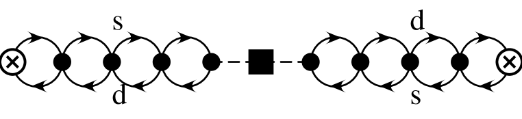
Figure 2: The leading $1/N_{c}$ contribution to $\Pi_{\Delta S=2}(q^{2})$ in the NJL model. Symbols as in fig. 1 except that a dot is now a NJL-vertex and the full lines are constituent quark-lines. The flavour is mentioned next to the lines.

In terms of the mixed pseudoscalar-axial-vector two-point function $\Pi_{P\mu}(q)_{sd}$ (see [17] for definition), the result is

$${}\Pi_{\Delta S=2}(q^{2})=-\frac{\displaystyle 1}{\displaystyle 2}\Pi_{P}^{\mu}(-q)_{sd}\Pi_{P\mu}(q)_{sd}\ .$$ (15)

This mixed two-point function has been calculated in the full ENJL model in the chiral limit [17] and in [21] for non-zero quark masses to all orders in the chiral expansion. The lowest order term in the expansion of the result in (15) coincides with that in (11) when the parameters are those determined from the NJL model.

At the non-factorizable level life becomes a lot more complicated. There are two major classes of diagrams in the leading contribution to the non-factorizable case. They are depicted in figs. 3 and 4, we will refer to these as 3-point and 4-point diagrams respectively.

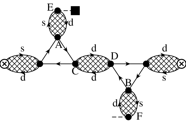
Figure 3: The class of 3-point diagrams. Symbols as in fig. 2, the hatched areas are a summation over sets of one-loop diagrams as shown in fig. 2.

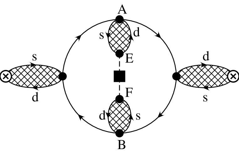
Figure 4: The class of 4-point diagrams, symbols as in fig. 3.

In addition the diagram of fig. 3 also exists with everywhere the quarks s and d interchanged and the directions of all fermion lines reversed. The latter diagram can then related to the first version by CPS-symmetry and can be calculated using the same code written for the diagram of fig. 3 but with the quark masses $m_{s}$ and $m_{d}$ interchanged. We have checked that diagram in fig. 4 gives the same result after that interchange. The tails here can be 0,1,2,3,… loops and they can be resummed using the procedure given in [17]. The expressions needed for the tails are given in [21]. They represent in a sense the fermionic equivalent of the propagators of the mesons. Notice that the two-point functions needed also contain parts that do not have a pole. Here it can be seen where the main complexity of the calculation comes from. The $X$ boson has both vector and axial-vector couplings, the internal coupling of the tail to the 3 or 4 point quark loop can thus have 4 different Dirac structures. The three- and four-point functions themselves have a rather complicated momentum dependence and need an explicit numerical integration over the Feynman parameters to be evaluated. This makes it rather important to have several consistency checks on the final numerical result. We will describe the ones we have used below in addition to the interchange of masses on the 4-point diagram. We refer to the 3-point diagrams by the form of the insertion at places A,B,C and D and the 4-point ones by their insertions at A and B. This in turn fixes the insertion in the points E and F in both diagrams. As an example let us quote the expression for the PSSP 3-point diagram corresponding to the flavours in fig. 3,

$$\mathrm{<PSSP>} \equiv \frac{\displaystyle i}{\displaystyle 2}\left[1+g_{S}\Pi_{P}(q)_{sd}\right]^{2}\,g_{S}^{3}\,\int^{\mu}_{0}\frac{d^{4}r}{(2\pi)^{4}}\,\Pi_{P}^{\mu}(-q-r)_{ds}\Pi_{P\mu}(q+r)_{ds}$$ (16)

$$\times \overline{\Pi}^{sdd}_{PPS}(q+r,-r)\left[1+g_{S}\Pi_{S}(-r)_{dd}\right]\,\overline{\Pi}^{sdd}_{PPS}(-q-r,r)\ .$$

The others are considerably more involved. The two- and three-point functions here are defined with the notation used in [21]. The non-barred ones correspond to the full functions and the barred ones to the one loop expressions[17, 21]. We have made sure that the expressions for the underlying 3 and 4-point one-quark-loop expressions obey all the Ward identities that follow from the symmetry in the one-loop case for the most general case, all masses different. The current identities are satisfied with the constituent masses. At the present level there is no contribution from diagrams that produce a Levi-Civita symbol. These only contribute at the level considered here as soon as $G_{V}\neq 0$. A large fraction of the work was involved in making sure the 3- and 4-point one-loop functions were correct.

5 What happened to the Fierzed term ?

In the standard VIA we have $B_{K}(\mu)=\left(3/4\right)\left(1+1/N_{c}\right)$. From the diagram in fig. 2 we get $B_{K}(\mu)=3/4$ and the difference comes from the colour suppressed combination of attaching the operator $\Gamma_{\Delta S=2}$ to the quark lines. In terms of the $X$ boson propagator this type of contributions corresponds to taking the diagram of fig. 4 and replacing the lines connecting A-E and B-F by a pointlike insertion and sending the cut-off $\mu$ to infinity. We can then rearrange the integration over $r$ and the internal quark loop momenta such that the new integration variables have no mixed dependence in any of the quark propagators. We can now split the double integral into two independent parts. The expression for this diagram then reduces to the one in fig. 2 with an extra factor of $1/N_{c}$ in front obtaining the usual VIA result. One can wonder how good is the VIA (i.e., the Fierzing) when one introduces the cut-off $\mu$ in the $r$ momentum. The answer is that this $1/N_{c}$ is only reached for rather high values of the cut-off $\mu$.

Let us also see what happens in the context of chiral perturbation theory. In fact the same contribution appears in the CHPT calculation. It is the one depicted in fig. 1d. To the order we have calculated here (i.e. next-to-leading order) it is exactly zero, the vector-vector and axial-vector–axial-vector cancel exactly. It is only at higher orders in the CHPT expansion, when the vertex vector(vector-axial)–$X$ boson is the one coming from the $L_{10}$ term in the ${\cal O}(p^{4})$ chiral Lagrangian, when this contribution starts showing itself. This in fact allows us a rare check on a single diagram. The chiral calculation for the vector(axial-vector)–vector(axial-vector) piece gives (at NLO) a contribution of

$${\Pi_{\Delta S=2}}^{Fierz}_{VV(AA)}(q^{2})=(-)\,\frac{B_{0}^{2}F_{0}^{2}}{16\pi^{2}}\,4\,\frac{\mu^{4}}{q^{4}}\ .$$ (17)

In the NJL calculation, this agrees for small values of $\mu$ (up to about 0.35 GeV) well. For larger values of $\mu$ the contribution of this diagram is $(3/4)\,\epsilon$, with $\epsilon\approx$ 0.006, 0.03, 0.08, 0.1, 0.2 and 0.3 for $\mu=$ 0.3, 0.5, 0.7, 0.9, 1.1 and 1.5 GeV. As can be seen the Fierz term is slightly suppressed for the values of $\mu$ that are relevant in the next section.

6 Numerical results

We have studied three cases, namely, the chiral case mentioned above; the case with SU(3) symmetry breaking $m_{s}\neq m_{d}$ with the input parameters introduced in section 3 and the case with non-zero quark masses but with $m_{s}=m_{d}$ also introduced in section 3. The procedure we have followed to analyze the numerical results is the following. We fit the ratio between the correction and the leading $1/N_{c}$ result for a fixed scale $\mu$ to $a/q^{2}+b+cq^{2}$ which always gives a very good fit ($a$, $b$ and $c$ are $\mu$ dependent). Once we have this fit we can extrapolate our $B_{K}$ form factor (remember that we have calculated it for Euclidean $q^{2}$) to the physical $B_{K}$, i.e. to $q^{2}=m_{K}^{2}$.

Let us first treat the chiral or massless quarks case. Here a nontrivial check on the results is that the diagrams have a behaviour which sums to $1/q^{2}$. The individual contributions do not have this behaviour. In fact for our lowest $q^{2}$ the cancellations are rather significant. This cancelation happens point by point in the loop momentum ($r$) integral since there is an underlying chiral relation for the 4-point amplitude. Therefore we have used a deterministic numerical integration scheme to have all diagrams evaluated at the same internal momenta. This increases the accuracy in the sum beyond the accuracy in the separate diagrams since only the noncanceling contributions survive at all stages of the calculation. We also see here a small $q^{2}$ dependence in the $B_{K}$ form factor, this is for $B_{K}$ as defined above but with off-shell kaons.

In this case $a$ is compatible with zero as required by chiral symmetry. $b$ is the relevant contribution to $B_{K}$ since $m_{K}^{2}|_{\chi}=0$. The first three columns in table 1 are $\mu$, $B_{K}^{\chi}(\mu)$ and $\hat{B}_{K}^{\chi}$ for this case. For calculating $\hat{B}_{K}$ we use $a_{+}=-2/9$ and $\Lambda^{(3)}_{\overline{MS}}=250$ MeV which corresponds to $\alpha_{S}^{(1)}(1.5\ {\rm GeV})=0.39$.

$\mu$ (GeV)	$B_{K}^{\chi}(\mu)$	$\hat{B}{}_{K}^{\chi}$	$B_{K}^{m}(\mu)$	$B_{K}^{a}(\mu)$	$\hat{B}_{K}^{m}$	$B_{K}^{\rm eq}(\mu)$	$\hat{B}_{K}^{\rm eq}$
0.3	0.68	0.50	0.74	0.50	0.55	0.74	0.55
0.5	0.59	0.59	0.71	$-$0.44	0.71	0.72	0.72
0.7	0.53	0.58	0.69	$-$2	0.75	0.68	0.75
0.9	0.48	0.55	0.66	$-$3	0.76	0.65	0.75
1.1	0.45	0.54	0.64	$-$4	0.76	0.64	0.76

Table 1: Results for $B_{K}$ and $\hat{B}_{K}$.

For very small $\mu$ we also see agreement with the CHPT calculation given above with the values for $B_{0}$ and $F_{0}$ expected for our NJL input values. The matching with QCD leading logarithmic evolution, i.e. the stability of $\hat{B}_{K}$, is not very good in this case.

In the second case ($m_{s}\neq m_{d}$), because the chiral symmetry is broken, there is a possibility for contributions to $B_{K}(q^{2})$ that are not proportional to $q^{2}$, i.e. $a\neq 0$. In fact a CHPT calculation like the one above predicts precisely the presence of this type of terms. For small values of $q^{2}$ the part due to $a$ dominates even though it is only a small correction when extrapolating to the physical $B_{K}^{m}$ at $q^{2}=m_{K}^{2}$. This can be found in column 4. The fifth column is the form factor $B_{K}^{a}$ for $q^{2}=-0.001$ GeV² where the correction due to the $a$ term is sizeable. Notice the difference between these two columns. This same feature should be visible in the lattice calculations as soon as they are done with different quark masses. The invariant $\hat{B}_{K}^{m}$ for this case is in column 6.

In the the last case, i.e. $m_{d}=m_{s}$, which is similar to the present lattice QCD calculations, the fit gives $a=0$ to a good precision and the value of $B_{K}^{\rm eq}$ extracted is rather independent of $q^{2}$. The invariant $\hat{B}_{K}^{\rm eq}$ in this case is in column 8.

A reasonably stable value for $\hat{B}_{K}^{\chi}$ occurs for scales $\mu\approx(0.7\sim 1.1)$ GeV. But the difference with the massless case is numerically significant. We obtain

$$\hat{B}_{K}^{m}(m_{K}^{2}\approx 0.13~{}{\rm GeV}^{2})\approx 1.35\,\hat{B}_{K}^{\chi}(m_{K}^{2}=0)$$ (18)

for scales $\mu\approx(0.7\sim 1.1)~{}{\rm GeV}$.

7 Conclusions

We have studied a nonleptonic weak matrix element in a way where the short and long distance contributions are separated in a physically visible fashion through the $X$-boson propagator. This allows us to identify the rôle of $\mu$ across diagrams and to connect with the running in the short distance domain. We have done this in the NJL-model to all orders in momenta there. This gave us a result that has manifestly the correct chiral properties.

In view of the results of [18, 19, 21] we expect to get a good prediction for the effects of non-zero and different current quark masses. We see those and find a significant change due to both. For the extrapolation to the kaon pole the difference between the masses has a much smaller effect than the fact that they were non-zero. In order to compute $B_{K}$ in the general case a careful extrapolation to the poles was needed. The final correction to the $B_{K}$ parameter compared to its leading value of $3/4$ turns out to be rather small. The stability of $\hat{B}_{K}$ when quark masses are present, is around scales $\mu\approx(0.7\sim 1.1)$ GeV. For these scales one may expect that the contribution of spin 1 mesons (remember that only the spin 0 mesons are the ones included for $G_{V}=0$) is important. This may be implemented like in the case of the $\pi^{+}-\pi^{0}$ mass difference [15, 16, 17] by going to the full ENJL model with vector–axial-vector mesons included. This also will allow us to compare with the results of the next-to-leading $1/N_{c}$ corrections obtained in similar approaches [10]. We are studying now this case [20]. We are also studying whether we can use the present program to obtain more information about higher order terms in the chiral Lagrangian.

References

- [1] M.K. Gaillard and B.W. Lee, Phys. Rev. D10 (1974) 897.
- [2] J.F. Donoghue, E. Golowich and B.R Holstein, Phys. Lett. B119B (1982) 412.
- [3] J. Bijnens, H. Sonoda and M.B. Wise, Phys. Rev. Lett. 53 (1984) 2367.
- [4] A. Pich and E. de Rafael, Phys. Lett. 158B (1985) 477.
-
[5]
K.G. Chetyrkin, A.L. Kataev, A.B. Krasulin
and A.A. Pivovarov, Phys. Lett. B174 (1986) 104;
R. Decker, Nucl. Phys. B277 (1986) 661. -
[6]
W.A. Bardeen, A. Buras and J.-M. Gérard, Phys. Lett.
B211(1988)371;
J. -M. Gérard in [7]. - [7] Proceedings of the Ringberg Workshop on Hadronic Matrix Elements and Weak Decays, Ringberg, Germany, april 1988, eds. A.J. Buras, J.-M. Gérard and W. Huber, Nucl. Phys. B(Proc. Suppl.)7A(1989)
- [8] J. Prades, C.A. Dominguez, J.A. Peñarrocha, A. Pich and E. de Rafael, Z. Phys. C51 (1991) 287.
-
[9]
N. Bilić, C.A. Dominguez and B. Guberina,
Z. Phys. C39 (1988) 351;
R. Decker, in [7];
L.J. Reinders and S. Yazaki, Nucl. Phys. B288 (1987) 789. - [10] J.-M. Gérard, Acta Physica Polonica B21(1990)257.
-
[11]
P.B. Mackenzie, in Proc. of the 16th
Lepton-Photon Interactions Symposium (Ithaca, New York 1993),
P. Drell and D. Rubin (eds.) (AIP Press, New York 1994);
S.R. Sharpe, Nucl. Phys. B(Proc. Suppl.)34(1994)403;
N. Ishizuka, M. Fukugita, H. Mino, M. Okawa, Y. Shizawa and A. Ukawa, Phys. Rev. Lett. 71 (1993) 24. - [12] J. Kambor, J. Missimer and D. Wyler, Nucl. Phys. B346(1990)17.
- [13] C. Bruno, Phys. Lett. B320(1994)135.
- [14] A. Pich and E. de Rafael, Nucl. Phys. B358(1991)311.
- [15] W.A. Bardeen, J. Bijnens and J.-M. Gérard, Phys. Rev. Lett. 62(1989)1343.
- [16] J. Bijnens and E. de Rafael, Phys. Lett. B273(1991)483.
- [17] J. Bijnens, E. de Rafael and H. Zheng, Z. Phys. C62(1994)437.
- [18] J. Bijnens, C. Bruno and E. de Rafael, Nucl. Phys. B390(1993)501.
- [19] T. Hatsuda and T. Kunihiro, QCD phenomenology based on a chiral Lagrangian, UTHEP-270, to be published in Phys. Rep.
- [20] J. Bijnens and J. Prades, in preparation.
- [21] J. Bijnens and J. Prades, 2 and 3-point functions in the ENJL model, NORDITA 94/27 N,P (hep-ph/9403233), to be publ. in Z. Phys. C.
- [22] J. Bijnens and J. Prades, Phys. Lett. B320(1994)130.