Hydrodynamic Transport Coefficients in Relativistic Scalar Field Theory

Abstract

Hydrodynamic transport coefficients may be evaluated from first principles in a weakly coupled scalar field theory at arbitrary temperature. In a theory with cubic and quartic interactions, the infinite class of diagrams which contribute to the leading weak coupling behavior are identified and summed. The resulting expression may be reduced to a single linear integral equation, which is shown to be identical to the corresponding result obtained from a linearized Boltzmann equation describing effective thermal excitations with temperature dependent masses and scattering amplitudes. The effective Boltzmann equation is valid even at very high temperature where the thermal lifetime and mean free path are short compared to the Compton wavelength of the fundamental particles. Numerical results for the shear and the bulk viscosities are presented.

Submitted to Physical Review D.

I Introduction

Linear response theory provides a framework for calculating transport coefficients starting from first principles in a finite temperature quantum field theory. As reviewed below, the resulting “Kubo” formulae express the hydrodynamic transport coefficients in terms of the zero momentum, small frequency limit of stress tensor–stress tensor correlation functions[1]. One-loop calculations of transport coefficients using these Kubo formulae in a relativistic scalar $\phi^{4}$ theory have appeared previously[2, 3]. However, those calculations are wrong even in the weak coupling limit; they fail to include an infinite class of diagrams which contribute at the same order as the one-loop diagram. These multi-loop diagrams are not suppressed because powers of the single particle thermal lifetime compensate the explicit coupling constants provided by the interaction vertices.

In this paper, all diagrams which make leading order contribution to the viscosities in a weakly coupled relativistic scalar field theory with cubic and quartic interactions are identified. The diagrammatic rules needed to calculate the required finite temperature spectral densities of composite operator correlation functions were derived in a previous paper[5] (and are summarized below). The dominant diagrams are identified by counting the powers of the coupling constants which result from a given diagram, including those generated by near “on-shell” singularities which are cut-off by the single particle thermal lifetime.

For the calculation of the shear viscosity, certain cut “ladder” diagrams, corresponding to the contribution of elastic scatterings only, are found to make the leading order contributions. The geometric series of cut ladder diagrams is then summed by introducing a set of effective vertices which satisfy coupled linear integral equations. The resulting expression is then shown to reduce to a single integral equation, which is solved numerically.

For the calculation of the bulk viscosity, in addition to the leading order ladder diagrams, contributions from the next order diagrams containing inelastic scattering processes must also be summed. In general, the bulk viscosity is proportional to the relaxation time of the processes which restore equilibrium when the volume of a system changes[6]. For a system of a single component real scalar field, such processes involve inelastic scatterings which change the number of particles. Hence, diagrams corresponding to such processes must be included.

Boltzmann equations based on kinetic theory have traditionally been used to calculate transport properties of dilute weakly interacting systems. However, the validity of kinetic theory is restricted by the condition that the mean free path of the particles must be much larger than any other microscopic length scale. In particular, the mean free path must be large compared to the Compton wavelength of the underlying particle in order for the classical picture of particle propagation to be valid. A Boltzmann equation describing the fundamental particles cannot be justified when this condition fails to hold. Such is the case at extremely high temperature, where the mean free path scales as $1/T$.

No such limitation exists when starting from the fundamental quantum field theory. Nevertheless, it will be shown that the correct transport coefficients, in a weakly coupled theory, may also be obtained by starting from a Boltzmann equation describing effective single particle thermal excitations with temperature dependent masses and scattering amplitudes. This equivalence holds even for asymptotically large temperatures where both the thermal lifetime and mean free path are tiny compared to the zero temperature Compton wavelength. Hence, in a weakly coupled theory, although a kinetic theory description in terms of fundamental particles is only valid at low temperatures, a kinetic theory description of effective thermal excitations remains valid at all temperatures.

The effective kinetic theory result presented in this paper is valid through all temperatures in the weak coupling limit. At low temperatures, $T\ll m_{\rm phys}$, where $m_{\rm phys}$ is the physical mass of the underlying particles at zero temperature, most particles are non-relativistic. Hence, the effective theory reduces to non-relativistic kinetic theory at low temperatures. If the temperature is in the range $m_{\rm phys}\,\,\vbox{\hbox{$\buildrel\displaystyle<\over{\sim}$}}\,\,T\ll m_{\rm phys}/\sqrt{\lambda}$, where $\lambda$ is the quartic coupling constant, most particles are relativistic, but the thermal corrections to the mass and the scattering amplitude are negligible. Consequently, the viscosities at these temperatures can be calculated by a kinetic theory of relativistic particles with temperature independent mass and scattering amplitudes.

The most interesting temperatures are those where $T={\cal O}(m_{\rm phys}/\sqrt{\lambda})$. At these temperatures, the thermal correction to the mass is comparable to the zero temperature mass. For weak coupling, this temperature is also large enough that most excitations are highly relativistic. One might expect that the thermal correction to the mass would then be irrelevant. This is true for some physical quantities which are insensitive to soft momentum contributions, such as the shear viscosity. However, other quantities, such as the bulk viscosity, are sensitive to soft momenta. For such quantities, including the thermal correction to the mass and the scattering amplitude will be shown to be essential.

At very high temperature, $T\,\,\vbox{\hbox{$\buildrel\displaystyle>\over{\sim}$}}\,\,m_{\rm phys}/\lambda$, all mass scales, including the cubic coupling constant, other than the temperature are completely negligible, and consequently the theory reduces to the massless scalar theory with only a quartic interaction.

Through out this paper, we work with the Lagrangian

$$-{\cal L}={1\over 2}\phi(-\partial_{\tau}^{2}-\nabla^{2}+m_{0}^{2})\phi+{g\over 3!}\phi^{3}+{\lambda\over 4!}\phi^{4}\;.$$ (1)

It is assumed that $\lambda\ll 1$ and $g^{2}={\cal O}(\lambda m_{0}^{2})$, so that the theory is always weakly coupled. For simplicity, we also take $m_{0}^{2}>0$. Note that at tree level, $m_{0}$ can be regarded as the physical mass $m_{\rm phys}$. Portions of the analysis will begin by assuming pure quartic interactions, after which the additional contribution arising from cubic interactions will be considered. The remainder of the paper is organized as follows. A brief review of various background material is presented in section II. This material includes the definition of transport coefficients, basic linear response theory, diagrammatic “cutting” rules for the evaluation of spectral densities, and a summary of the behavior of self-energies at high temperature. Section III deals with the problem of identifying the leading order diagrams. By counting powers of coupling constants, including those from near on-shell singularities, ladder diagrams are identified as the leading order diagrams. The summation of these diagrams is discussed in section IV. Section V contains a brief review of the computations of viscosities starting from the Boltzmann equation, and then discusses the relation between the resulting formulae and those in section IV. Using the results of the previous sections, the final calculation of viscosities is discussed in section VI, and numerical results presented in section VII.

Several appendices contain technical details. Explicit forms of the imaginary-time and real-time propagators used in the main body of the paper are summarized in appendix A. Appendices B and C present explicit forms of the “ladder” kernels discussed in section IV. In appendix D, the first order correction to the equilibrium stress-energy tensor needed in sections IV and VI are calculated. Appendix E discusses the soft momentum and collinear contributions to finite temperature cut diagrams, and shows that they does not upset the estimates used in section III. Appendix F contains technical details of summing up the “chain” diagrams appearing in section III D.

II Background material

A Hydrodynamic transport coefficients

In a single component real scalar field theory, the only locally conserved quantities are energy and momentum. The transport coefficients associated with energy and momentum flow, known as the shear and bulk viscosities, may be defined by the following constitutive relation,

$$\langle T_{ij}\rangle\simeq-{\eta\over\langle\varepsilon{+}{\cal P}\rangle}\left(\nabla_{i}\langle T_{j}^{0}\rangle+\nabla_{j}\langle T_{i}^{0}\rangle-{\textstyle{2\over 3}}\delta_{ij}\nabla^{l}\langle T_{l}^{0}\rangle\right)-{\zeta\over\langle\varepsilon{+}{\cal P}\rangle}\delta_{ij}\nabla^{l}\langle T_{l}^{0}\rangle+\delta_{ij}\langle{\cal P}\rangle\;,$$ (2)

valid when the length scale of energy and momentum fluctuations is much longer than the mean free path. Here, $T_{ij}$ is the spatial part of the stress-energy tensor $T_{\mu\nu}$, $\varepsilon\equiv T_{00}$ is the energy density, ${\cal P}={1\over 3}T_{i}^{i}$ is the pressure, and $\eta$ and $\zeta$ are the shear and the bulk viscosities, respectively. Also, $\langle\cdots\rangle$ denotes the expectation in a non-equilibrium thermal ensemble describing a system slightly out of equilibrium. Since there are no additional conserved charges, thermal conductivity is not an independent transport coefficient.

The above constitutive relation, combined with the exact conservation equation

$$\partial_{\mu}T^{\mu\nu}(x)=0\;,$$ (3)

constitute linearized hydrodynamic equations for a relativistic fluid. With the help of the equilibrium thermodynamic relation

$${\partial\langle{\cal P}\rangle_{\rm eq}\over\partial\langle\varepsilon\rangle_{\rm eq}}=v_{\rm s}^{2}\;,$$ (4)

where $v_{\rm s}$ is the speed of sound, the linearized hydrodynamic equations can be reduced to two equations for the transverse part of the momentum density $\langle\pi_{T}^{\vphantom{x}}\rangle$ and the pressure $\langle{\cal P}\rangle$,

$$\displaystyle(\partial_{t}-D\nabla^{2})\,\langle\pi_{T}^{\vphantom{x}}(x)\rangle=0\;,$$ (6)

and (7)

$$\displaystyle\left(\partial_{t}^{2}-v_{\rm s}^{2}\nabla^{2}-\Gamma\nabla^{2}\partial_{t}\right)\langle{\cal P}(x)\rangle=0 \;.$$

Here the diffusion constant $D$ is proportional to the shear viscosity

$$D \equiv \displaystyle\eta/\langle\varepsilon{+}{\cal P}\rangle_{\rm eq}\;,$$ (8)

and the sound attenuation constant $$\Gamma$$ equals a linear combination of the viscosities

$$\Gamma \equiv \displaystyle({\textstyle{4\over 3}}\eta{+}\zeta)/\langle\varepsilon{+}{\cal P}\rangle_{\rm eq}\;.$$ (9)

Using the basic linear response result, one may express the viscosities in terms of the stress tensor-stress tensor correlation functions[1, 8]. One finds the “Kubo” formulae,

$$\displaystyle\eta={\beta\over 20}\lim_{\omega\to 0}\lim_{{\bf q}\to 0}\sigma_{\pi\pi}^{\vphantom{x}}(\omega,{\bf q})\;,$$ (11)

$$\displaystyle\zeta={\beta\over 2}\lim_{\omega\to 0}\lim_{{\bf q}\to 0}\sigma_{\bar{\cal P}\bar{\cal P}}^{\vphantom{x}}(\omega,{\bf q})\;.$$ (12)

Here $\sigma_{\pi\pi}^{\vphantom{x}}(\omega,{\bf q})$ is the Fourier transformed traceless stress-stress Wightman function,

$$\displaystyle\sigma_{\pi\pi}^{\vphantom{x}}(\omega,{\bf q})\equiv\int d^{3}{\bf x}\,dt\,e^{-i{\bf q}{\cdot}{\bf x}+i\omega t}\,\langle\pi_{lm}(t,{\bf x})\pi^{lm}(0)\rangle_{\rm eq}\;,$$ (13)

where (14)

$$\displaystyle\pi_{lm}(x)\equiv T_{lm}(x)-{\textstyle{1\over 3}}\delta_{lm}T_{i}^{i}(x)\;$$

is the traceless stress tensor. Similarly,

$$\displaystyle\sigma_{\bar{\cal P}\bar{\cal P}}^{\vphantom{x}}(\omega,{\bf q})\equiv\int d^{3}{\bf x}\,dt\,e^{-i{\bf q}{\cdot}{\bf x}+i\omega t}\,\langle\bar{\cal P}(t,{\bf x})\bar{\cal P}(0)\rangle_{\rm eq}\;,$$ (15)

where (16)

$$\displaystyle\bar{\cal P}(t,{\bf x})\equiv{\cal P}(t,{\bf x})-v^{2}{\varepsilon}(t,{\bf x})={\textstyle{1\over 3}}T_{i}^{i}(x)-v^{2}T_{00}(x)\;,$$

is a linear combination of pressure and energy density. The constant $v^{2}$ in this combination is arbitrary; due to energy-momentum conservation, Wightman functions involving the energy density vanish (at non-zero frequency) in the zero spatial momentum limit. However, as will be discussed in section IV, $v$ will eventually be chosen to equal the speed of sound. This will be necessary in order to make the final integral equation for the transport coefficient well defined. Note that, whereas the approximate constitutive relation (2) involves a non-equilibrium thermal expectation, the Kubo formulae (II A) express the transport coefficients solely in terms of equilibrium expectation values.

B Qualitative behavior of the viscosities

In general, a transport coefficient is roughly proportional to the mean free path, or equivalently the relaxation time, of the processes responsible for the particular transport[6].

This behavior is most easily seen in a diffusion constant (or in the shear viscosity). Consider a system with a conserved charge. In such a system, the diffusion of a charge density fluctuation may be modeled by a random walk[8]. The rate of the diffusion then depends on two parameters; the step size (the mean free path) and the number of steps per time (the mean speed). A longer step size or a larger number of steps per time implies faster diffusion of the excess charge, i.e., a larger diffusion constant $D$. Since the diffusion constant has the dimension of a length, one finds

$$D\sim l_{\rm free}\bar{v}\;.$$ (17)

Recall that the diffusion constant in Eq. (8) is given by $D=\eta/\langle\varepsilon{+}{\cal P}\rangle_{\rm eq}$. Applying the above estimate of $D$ yields

$$\eta\sim l_{\rm free}\bar{v}\langle\varepsilon{+}{\cal P}\rangle_{\rm eq}\;.$$ (18)

Given the scattering cross-section $\sigma$ and the density of the particles $n$, the mean free path can be estimated as $l_{\rm free}\sim 1/n\sigma$. Consider a weakly coupled scalar $\lambda\phi^{4}$ theory. The lowest order scattering cross section in the $\lambda\phi^{4}$ theory is $\sigma\sim\lambda^{2}/s$ where $s$ is the square of the center of mass energy. At high temperature, $T\gg m_{\rm phys}$, the only relevant mass scale is the temperature. (Here $m_{\rm phys}$ denotes the physical mass.) Hence, $\sigma\sim\lambda^{2}/T^{2}$, $n\sim T^{3}$, and

$$\eta\sim T^{3}/\lambda^{2}\qquad(T\gg m_{\rm phys})\;.$$ (19)

At low temperature, $T\ll m_{\rm phys}$, $\sigma\sim\lambda^{2}/m_{\rm phys}^{2}$ and $\bar{v}\sim(T/m_{\rm phys})^{1/2}$. At these temperatures, the energy density $\langle\varepsilon\rangle_{\rm eq}\sim m_{\rm phys}n$, dominates over the pressure. Canceling two density factors in $l_{\rm free}$ and $\langle\varepsilon\rangle_{\rm eq}$, the shear viscosity can be estimated as

$$\eta\sim m_{\rm phys}^{3}(T/m_{\rm phys})^{1/2}/\lambda^{2}\qquad(T\ll m_{\rm phys})\;.$$ (20)

Note that the shear viscosity is not analytic in the weak coupling constant. This may be taken as an indication that the first few terms in the usual Feynman diagram expansion cannot produce the correct value of the leading order shear viscosity.

For the bulk viscosity, the situation is more complicated than the simple picture given above. The bulk viscosity does not have an interpretation as a diffusion constant. Hence, the random walk model cannot be directly applied. The bulk viscosity is still proportional to the mean free time (inverse transition rate) of a scattering process since the viscosities govern relaxation of a system towards equilibrium. However, the factors multiplying the mean free time cannot simply be $\langle\varepsilon{+}{\cal P}\rangle_{\rm eq}$ since the bulk viscosity $\zeta$ vanishes in a scale invariant system[9].

To understand this, consider a slow uniform expansion of the volume of a system. In such an expansion, there can be no shear flow[10]. Hence, the relaxation of disturbances caused by the expansion depends only on the bulk viscosity. For scale invariant systems, the restoration of local equilibrium does not require any relaxation process. A suitable scaling of the temperature alone can maintain local equilibrium at all times. Hence, for such systems, including the non-relativistic monatomic ideal gas and the ideal gas of massless particles, the bulk viscosity vanishes since the relaxation time vanishes.

When the system is not scale invariant, the bulk viscosity must be proportional to a measure of the violation of scale invariance, or the mass $m_{\rm phys}$. In section IV, the formula for the leading order bulk viscosity at high temperature is shown to be

$$\zeta\sim m_{\rm phys}^{4}\tau_{\rm free}\;.$$ (21)

The mean free time $\tau_{\rm free}$ here is given by the inverse of the transition rate per particle,

$$\tau_{\rm free}\equiv n/(dW/dVdt)\;,$$ (22)

where $dW/dVdt$ the transition rate per volume. corresponding to the relaxation of the uniformly expanding system. In a number non-conserving system with broken scale invariance (such as a massive scalar theory), the number-changing inelastic scattering processes are ultimately responsible for relaxation towards equilibrium. As the system expands, the temperature must decrease since the system loses energy pushing the boundary. Decreasing energy implies decreasing particle number in a number non-conserving system with broken scale invariance. Hence, the relaxation toward equilibrium must involve number-changing scatterings. In the $g\phi^{3}{+}\lambda\phi^{4}$ theory, the lowest order number-changing process is 2–3 scatterings involving 3 cubic vertices or 1 cubic and 1 quartic vertices. In pure $\lambda\phi^{4}$ theory, the lowest order number changing process is 2–4 scatterings involving 2 quartic vertices.

At high temperature, $m_{\rm phys}\ll T\,\,\vbox{\hbox{$\buildrel\displaystyle<\over{\sim}$}}\,\,m_{\rm phys}/\sqrt{\lambda}$, most particles have momentum of ${\cal O}(T)$. However, due to the Bose-Einstein enhancement, the transition rate per volume will be shown to be dominated by the ${\cal O}(m_{\rm th})$ momentum components in the system where $m_{\rm th}$ is the thermal mass containing ${\cal O}(\sqrt{\lambda}T)$ thermal corrections. In the $g\phi^{3}{+}\lambda\phi^{4}$ theory, with the statistical factors for 5 particles involved in the scattering, the transition rate per volume is ${\cal O}(\lambda^{2}g^{2}T^{5}/m_{\rm th}^{3})$ which is ${\cal O}(T^{3}/m_{\rm th}^{3})$ larger than the transition rate of the particles with ${\cal O}(T)$ momentum. Hence at temperatures in the range $m_{\rm phys}\ll T\,\,\vbox{\hbox{$\buildrel\displaystyle<\over{\sim}$}}\,\,m_{\rm phys}/\sqrt{\lambda}$, the bulk viscosity will be

$$\zeta\sim m_{\rm phys}^{4}m_{\rm th}^{3}/\lambda^{2}g^{2}T^{2}\;.$$ (23)

When $T={\cal O}(m_{\rm phys}/\sqrt{\lambda})$, $\zeta={\cal O}(T^{3}/\sqrt{\lambda})$ which is ${\cal O}(\lambda^{3/2})$ smaller than the shear viscosity. At the same temperature, the $\lambda\phi^{4}$ theory transition rate per volume is ${\cal O}(\lambda^{3}T^{4})$ again due to the Bose-Einstein enhancement. In this case, $\zeta={\cal O}(\beta m_{\rm phys}^{4}/\lambda^{3})={\cal O}(T^{3}/\lambda)$ which is ${\cal O}(\lambda)$ smaller than the shear viscosity.

At very high temperature $T\gg m_{\rm phys}/\lambda$, all mass scales, including the cubic coupling constant, other than the temperature are completely negligible, and consequently the theory reduces to the massless scalar theory with only a quartic interaction. The massless scalar theory is classically scale invariant. However, quantum mechanics breaks the scale invariance. The measure of the violation of scale invariance in this case is the renormalization group $\beta$-function. Since the transition rate per volume must still be ${\cal O}(\lambda^{3}T^{4})$ due to the thermally generated ${\cal O}(\sqrt{\lambda}T)$ mass, the bulk viscosity in this case is ${\cal O}(T^{3}\beta(\lambda)^{2}/\lambda^{3})={\cal O}(\lambda T^{3})$.

At low temperature, $T\ll m_{\rm phys}$, the bulk viscosity is proportional to the mean free time and the number density. At these temperatures, the transition rate per volume in the $g\phi^{3}{+}\lambda\phi^{4}$ theory is ${\cal O}(e^{-3\beta m_{\rm phys}})$, since the center of mass energy must exceed $3m_{\rm phys}$ for a 2–3 process to occur. Since the density $n={\cal O}(e^{-\beta m_{\rm phys}})$ at low temperature, the bulk viscosity is then ${\cal O}(e^{\beta m_{\rm phys}}/\lambda^{3})$. The bulk viscosity at low temperature is hence much larger than the ${\cal O}(1/\lambda^{2})$ shear viscosity. In the $\lambda\phi^{4}$ theory, the transition rate is ${\cal O}(e^{-4\beta m_{\rm phys}})$ since the center of mass energy in this case must exceed $4m_{\rm phys}$ for a 2–4 process to occur. The bulk viscosity is then ${\cal O}(e^{2\beta m_{\rm phys}}/\lambda^{4})$, and again much larger than the shear viscosity.

C Linear response theory

Linear response theory describes the behavior of a many-body system which is slightly displaced from equilibrium. First order time dependent perturbation theory implies that[8]

$$\delta\langle\hat{A}_{a}(t,{\bf x})\rangle=i\int d^{3}{\bf x}^{\prime}\!\int_{-\infty}^{t}dt^{\prime}\,\langle[\hat{A}_{a}(t,{\bf x}),\hat{A}_{b}(t^{\prime},{\bf x}^{\prime})]\rangle_{\rm eq}\,F_{b}(t^{\prime},{\bf x}^{\prime})\;,$$ (24)

where $\{F_{b}(t,{\bf x})\}$ is some set of generalized external forces coupled to the interaction picture charge density operators $\{\hat{A}_{b}(t,{\bf x})\}$ so that

$$\delta\hat{H}(t)=-\int d^{3}{\bf x}\,F_{b}(t,{\bf x})\,\hat{A}_{b}(t,{\bf x})\;,$$ (25)

and $\langle\cdots\rangle_{\rm eq}$ denotes an equilibrium thermal expectation. (Summation over the repeated index $b$ should be understood.)

To examine transport properties, it is convenient to consider a relaxation process in which the external field is held constant for a long time (allowing the system to re-equilibrate in the presence of the external field), and then suddenly switched off,

$$F_{b}(t,{\bf x})\equiv F_{b}({\bf x})\,e^{\epsilon t}\,\theta(-t)\;,$$ (26)

where $\epsilon$ is a positive infinitesimal number. Once the field is switched off, the system will relax back towards the original unperturbed equilibrium state. Spatial translational invariance implies that Fourier components of the initial values $\delta\langle\hat{A}_{a}(0,{\bf x})\rangle$ are linearly related to the Fourier components of $F_{b}({\bf x})$. Hence, after a Fourier transform in space and a Laplace transform in time, Eq. (24) turns into an algebraic relation[8],

$$\delta\tilde{A}_{a}(z,{\bf k})={1\over iz}[\chi_{ab}^{\vphantom{x}}(z,{\bf k})\,\chi_{bc}^{-1}(i\epsilon,{\bf k})-\delta_{ac}]\delta\tilde{A}_{c}(t{=}0,{\bf k})\;,$$ (27)

where $\delta\tilde{A}_{a}(z,{\bf k})$ are Laplace and Fourier transformed deviations from equilibrium values $\delta\langle\hat{A}_{a}(t,{\bf x})\rangle$, and $\delta\tilde{A}_{c}(t{=}0,{\bf k})$ are Fourier transformed initial values $\delta\langle\hat{A}_{c}(t{=}0,{\bf x})\rangle$. Here, $\chi_{ab}^{\vphantom{x}}(z,{\bf k})$ is the retarded correlation function with complex frequency $z$; it has the spectral representation

$$\chi_{ab}^{\vphantom{x}}(z,{\bf k})=\int{d\omega\over 2\pi}\,{\rho_{ab}^{\vphantom{x}}(\omega,{\bf k})\over\omega-z}\;,$$ (28)

where the spectral density is

$$\rho_{ab}^{\vphantom{x}}(\omega,{\bf k})\equiv\int d^{4}x\,e^{-i{\bf k}{\cdot}{\bf x}+i\omega t}\,\langle[\hat{A}_{a}(t,{\bf x}),\hat{A}_{b}(0)]\rangle_{\rm eq}\;.$$ (29)

If $\hat{A}_{a}$’s are conserved charge densities, then Ward identities can be shown to imply that the response functions have hydrodynamic poles (poles in the frequency plain which vanish as the spatial momentum goes to zero)[11]. In the case of the conserved energy and momentum densities, the response functions in Eq. (27) can be shown to have a pole at $z=-iD{\bf k}^{2}$ when the disturbed charge is the transverse part of the momentum density $\pi_{T}^{\vphantom{x}}$, and poles at $z^{2}=v^{2}{\bf k}^{2}-i\Gamma z{\bf k}^{2}$ when the disturbed charge is the energy density or the longitudinal part of the momentum density.

Eq. (27) solves the initial value problem in terms of the response function. When the conserved quantities are energy and momentum densities, the time evolution of the initial values can be also described (for low frequency and momentum) by the phenomenological hydrodynamic equations (II A). When Fourier transformed in space and Laplace transformed in time, Eqs. (II A) yield response functions with exactly the same diffusion and sound poles. Hence, by extracting the diffusion constant $D$ and the sound attenuation constant $\Gamma$ from the pole positions in the correlation functions, one may derive the Kubo formulae (II A) for the viscosities.

The Wightman functions appearing in formulae (II A) for the viscosities are trivially related to the corresponding spectral densities:

$$\rho_{\pi\pi}^{\vphantom{x}}(\omega,{\bf q}) \displaystyle= \displaystyle(1-e^{-\beta\omega})\,\sigma_{\pi\pi}(\omega,{\bf q})$$ (30)

$$\rho_{\bar{\cal P}\bar{\cal P}}^{\vphantom{x}}(\omega,{\bf q}) \displaystyle= \displaystyle(1-e^{-\beta\omega})\,\sigma_{\bar{\cal P}\bar{\cal P}}(\omega,{\bf q})\;.$$ (31)

Hence, the viscosities can equivalently be written as zero frequency derivatives of spectral densities,

$$\displaystyle\eta={1\over 20}\,\lim_{\omega\to 0}\,\lim_{{\bf q}\to 0}\,{\partial\over\partial\omega}\rho_{\pi\pi}(\omega,{\bf q})\;,$$ (33)

and (34)

$$\displaystyle\zeta={1\over 2}\,\lim_{\omega\to 0}\,\lim_{{\bf q}\to 0}\,{\partial\over\partial\omega}\rho_{\bar{\cal P}\bar{\cal P}}(\omega,{\bf q})\;.$$

D Cutting rules

In Ref.[5], diagrammatic cutting rules for the perturbative calculation of the spectral density of an arbitrary two-point correlation function were derived starting from imaginary time finite temperature perturbation theory. These rules are a generalization of the standard zero-temperature Cutkosky rules, to which they reduce as temperature goes to zero.

To calculate the perturbative expansion of a finite temperature spectral density, one should draw all cut Feynman diagrams for the two-point correlation function of interest.

FIG. 1.: A typical cut diagram in a scalar $\lambda\phi^{4}$ theory.

All cuts that separate the two external operators are allowed at non-zero temperature. Each line corresponds to either a cut or uncut thermal propagator, as described below.

A typical example of a finite temperature cut diagram is shown in Fig. 1. Note that a cut at finite temperature can separate a diagram into multiple connected pieces, some of which are disconnected from the external operators. A disconnected piece, such as the portion labeled A in Fig. 1, cannot contribute in a zero temperature cut diagram because of energy momentum conservation. For example, at zero temperature the piece labeled A would represent an impossible event of four incoming on-shell physical particles scattering and disappearing altogether. However, at finite temperature there exist physical thermal excitations in the medium. Thus, the above disconnected piece also represents the elastic scattering of a particle off of a thermal excitation already present in the medium. This scattering process is clearly possible; the amplitude is proportional to the density of the thermal particles (as the form of the cut propagator shown below clearly indicates).

An uncut line in the unshaded region corresponds to a real-time time-ordered propagator $\langle{\cal T}(\phi(x)\phi(0))\rangle$, an uncut propagator in the shaded region is $\langle{\cal T}(\phi(x)\phi(0))\rangle^{*}$, and a cut line corresponds to the Wightman function $\langle\phi(x)\phi(0)\rangle$. In momentum space, the uncut propagator has the following spectral representation

$$\tilde{G}(k)\equiv\int{d\omega\over 2\pi}\,[1{+}n(\omega)]\,\rho(\omega,|{\bf k}|)\left({2i\omega\over(k^{0})^{2}-(\omega{-}i\epsilon)^{2}}\right)\;,$$ (35)

where $\rho(\omega,|{\bf k}|)$ is the single particle spectral density. The cut propagator is proportional to the single particle spectral density

$$S(k)\equiv[1{+}n(k^{0})]\,\rho(k)\;,$$ (36)

where $n(k^{0})$ is the Bose statistical factor $1/(e^{k^{0}\beta}{-}1)$. In more physical terms,

$$dV(k)\equiv\theta(k^{0})\,S(k)\,{d^{4}k\over(2\pi)^{4}}=\theta(k^{0})\,[1{+}n(k^{0})]\,\rho(k)\,{d^{4}k\over(2\pi)^{4}}\;$$ (37)

is the thermal phase space volume available to a final state particle in a scattering process, and

$$dN(k)\equiv\theta(-k^{0})\,S(k)\,{d^{4}k\over(2\pi)^{4}}=\theta(k^{0})\,n(k^{0})\,\rho(k)\,{d^{4}k\over(2\pi)^{4}}\;$$ (38)

is the number of thermal excitations within the 4-momentum range $(k_{\mu},k_{\mu}{+}dk_{\mu})$.

If the single particle spectral density is approximated by a delta function (to which it reduces at zero temperature), i.e.,

$$\rho_{\rm free}^{\vphantom{x}}(k)={\rm sgn}(k^{0})\,2\pi\delta(k^{2}+m_{0}^{2})\;,$$ (39)

then self-energy insertions on any line generate ill-defined products of on-shell delta functions. Although these on-shell singularities disappear when all cut diagrams are summed, it is far more convenient to first resum single particle self-energy insertions. The resummed single particle spectral density $\rho(k)$ will then include the thermal lifetime of single particle excitations, which will smear the $\delta$-function peaks and produce a smooth spectral density. Henceforth, all single particle propagators will include the thermal self-energy and no self-energy insertions will appear explicitly in any cut diagram.

E Propagators and self-energies at high temperature

To analyze near infrared singularities, the explicit forms of single particle propagators will be needed. The resummed single particle spectral density can be calculated as

FIG. 2.: One-loop self-energy diagrams in a scalar $g\phi^{3}{+}\lambda\phi^{4}$ theory. At high temperatures, the diagrams (a) and (b) produce a thermal mass squared of order $\lambda T^{2}$. The contribution of the diagram (c) to the thermal mass is ${\cal O}(g^{2}T/m_{\rm th})={\cal O}(\lambda^{3/2}T^{2})$.

the discontinuity of the analytically continued imaginary-time propagator across the real frequency axis,

$$\rho(k) = \displaystyle-i\left(\tilde{G}_{E}(k^{0}{+}i\epsilon,{\bf k})-\tilde{G}_{E}(k^{0}{-}i\epsilon,{\bf k})\right)$$ (40)

$$= \displaystyle{-i\over k^{2}+m_{\rm th}^{2}+\Sigma(k)}+{i\over k^{2}+m_{\rm th}^{2}+\Sigma(k)^{*}}$$ (41)

$$= \displaystyle-iG_{R}(k)+iG_{A}(k)={2\Sigma_{I}(k)\over|k^{2}+m_{\rm th}^{2}+\Sigma(k)|^{2}}\;,$$ (42)

where the subscript $R$ indicates the retarded propagator given by the analytic continuation of the Euclidean propagator

$$G_{R}(k)=\tilde{G}_{E}(k^{0}{+}i\epsilon,{\bf k})\;,$$ (43)

and the subscript $A$ indicates the advanced propagator defined similarly, but with $k^{0}{-}i\epsilon$ instead of $k^{0}{+}i\epsilon$[12, 13]. Here, the thermal mass $m_{\rm th}$ includes the ${\cal O}(\lambda T^{2})$ one-loop corrections shown in Fig. 2, and $\Sigma(k)$ is the analytically continued single particle self-energy

$$\Sigma(k)\equiv\Sigma_{E}(k^{0}{+}i\epsilon,{\bf k})=\Sigma_{R}(k){-}i\Sigma_{I}(k)\;.$$ (44)

The thermal mass squared $m_{\rm th}^{2}$ may be defined by the (off-shell) condition $\Sigma_{R}(0)\equiv 0$. Also, note that since $\rho(k)$ is the spectral density of a correlation function of the CPT even Hermitian operators $\hat{\phi}$, $\rho(k)$ must be an odd function of the frequency $k^{0}$[5, 8]. This implies that $\Sigma_{I}(k)$ is also an odd function of $k^{0}$.

As will be reviewed below, the imaginary part of the self-energy is ${\cal O}(\lambda^{2})$, and so is small for weak coupling. Hence, the definition (42) shows that the spectral density in the weak coupling limit has sharp peaks near $k^{0}=\pm E_{k}$, where the effective single particle energy $E_{k}$ satisfies the dispersion relation

$$E_{k}^{2}={\bf k}^{2}+m_{\rm th}^{2}+\Sigma_{R}(E_{k},|{\bf k}|)\;.$$ (45)

Near the peaks, the spectral density may be approximated by a combination of two Lorentzians,

$$\rho(k)={1\over 2E_{k}}\,\left({2\Gamma_{k}\over(k^{0}{-}E_{k})^{2}+\Gamma_{k}^{2}}-{2\Gamma_{k}\over(k^{0}{+}E_{k})^{2}+\Gamma_{k}^{2}}\right)\times\left(1+{\cal O}(\lambda^{2})\right)\;,$$ (46)

where $\Gamma_{k}$ is the momentum dependent thermal width given by

$$\Gamma_{k}\equiv\Sigma_{I}(E_{k},|{\bf k}|)/2E_{k}\;.$$ (47)

The thermal width $\Gamma_{k}$ is always positive since $\Sigma_{I}(k)$, or equivalently the single particle spectral density, must be positive for positive frequencies. This can be easily seen from the relation between the spectral density and the Wightman function and the positivity of the (Fourier transformed) Wightman function $\langle\phi(x)\phi(0)\rangle$[12]. Note that altogether $\rho(k)$ has four poles at $k^{0}=E_{k}{\pm}i\Gamma_{k}$ and $k^{0}=-E_{k}{\pm}i\Gamma_{k}$. In terms of the single particle spectral density, the cut propagator is

$$S(k)=[1{+}n(k^{0})]\,\rho(k)={2\,[1{+}n(k^{0})]\,\Sigma_{I}(k)\over\left|k^{2}+m_{\rm th}^{2}+\Sigma(k)\right|^{2}}\;.$$ (48)

For the uncut propagator given by Eq. (35), the frequency integral can be exactly carried out to yield (see appendix A for details)

$$\tilde{G}(k) = \displaystyle-i{1+n(k^{0})\over k^{2}+m_{\rm th}^{2}+\Sigma(k)}+i{n(k^{0})\over k^{2}+m_{\rm th}^{2}+\Sigma(k)^{*}}$$ (50)

$$= \displaystyle-i{k^{2}+m_{\rm th}^{2}+\Sigma_{R}(k)\over\left|k^{2}+m_{\rm th}^{2}+\Sigma(k)\right|^{2}}+{\coth(k^{0}\beta/2)\over 2}\,\rho(k)\;.$$ (51)

In the weak coupling limit, this becomes

$$\tilde{G}(k)=\left(-i{1+n(E_{k})\over(E_{k}{-}i\Gamma_{k})^{2}-k^{2}_{0}}+i{n(E_{k})\over(E_{k}{+}i\Gamma_{k})^{2}-k^{2}_{0}}\right)\times\left(1+{\cal O}(\lambda^{2})\right)\;.$$ (52)

The first term in Eq. (52) has poles at $k^{0}=\pm(E_{k}{-}i\Gamma_{k})$, and the second term has poles at $k^{0}=\pm(E_{k}{+}i\Gamma_{k})$, coinciding with the pole positions of the spectral density $\rho(k)$.

FIG. 3.: Cut two-loop self-energy diagrams in a scalar $g\phi^{3}{+}\lambda\phi^{4}$ theory which produce a thermal width of order $\lambda^{2}T$.

An important point to notice is that even though the statistical factor $n(k^{0})$ has a pole at $k^{0}=0$, both the cut propagator $S(k)$ and the uncut propagator $\tilde{G}(k)$ are finite at zero frequency since the self-energy $\Sigma_{I}(k)$, which is an odd function of $k^{0}$, vanishes at $k^{0}=0$. Hence, although numerous factors of the statistical factors may appear in an expression for a diagram, one can be sure that there is no pole when loop frequencies approach zero.

To determine the size of the thermal mass $m_{\rm th}$ and the thermal width $\Gamma_{k}$ at high temperatures, the size of the one-loop (Fig. 2) and the two-loop (Fig. 3) self-energies at on-shell momenta must be known. At relativistic temperatures, $T\,\,\vbox{\hbox{$\buildrel\displaystyle>\over{\sim}$}}\,\,m_{0}$, the first one-loop diagram, Fig. 2a, generates an ${\cal O}(\lambda T^{2})$ contribution to the real part of the self-energy. Diagram 2b, with two cubic interaction vertices, is ${\cal O}(g^{2}T^{2}/m_{\rm th}^{2})$ which is at most ${\cal O}(\lambda T^{2})$ since by assumption $g={\cal O}(\sqrt{\lambda}m_{0})$, and $m_{\rm th}\geq m_{0}$. At high temperature, the real part of diagram Fig. 2c is ${\cal O}(g^{2}\ln(T/m_{\rm th}))$ which is at most ${\cal O}(\lambda^{2}T^{2}\ln\lambda)$. Hence, the diagram 2c does not contribute to the leading weak coupling behavior of the thermal mass correction. Hence, the thermal mass is of order

$$m_{\rm th}=\sqrt{m_{0}^{2}+{\cal O}(\lambda T^{2})}\sim\sqrt{\lambda}T\;$$ (53)

when $T\,\,\vbox{\hbox{$\buildrel\displaystyle>\over{\sim}$}}\,\,m_{0}/\sqrt{\lambda}$.

The imaginary part of the self-energy receives an ${\cal O}(g^{2}T^{2})$ contribution from the one-loop diagram 2c, but this contribution vanishes for on-shell external momenta since an on-shell excitation of mass $m_{\rm th}$ cannot decay into two on-shell excitations with the same mass. (Nor can an on-shell excitation absorb the momentum of a thermal excitation and remain on-shell.) Hence, the dominant contribution to the on-shell imaginary part of the self-energy comes from the two-loop diagrams shown in Fig. 3. At high temperature, these two-loop diagrams produce a ${\cal O}(\lambda^{2}T^{2})$ imaginary part of the self-energy. Consequently, at high temperature, the thermal width $\Gamma_{k}$, as defined in Eq. (47), is ${\cal O}(\lambda^{2}T)$ for hard (compared to $m_{\rm th}$) external on-shell momenta, and ${\cal O}(\lambda^{3/2}T)$ for soft on-shell momenta.

III Classification of diagrams

A Near on-shell singularities of cut diagrams

Diagrams contributing to the spectral density of the stress tensor correlations function have two external vertices each of which connect to at least two propagators. For example, the shear viscosity requires evaluating the correlation function

$$\sigma_{\pi\pi}=\langle{\pi}_{lm}{\pi}^{lm}\rangle\;,$$ (54)

where the traceless stress tensor,

$${\pi}_{lm}\equiv\partial_{l}{\phi}\,\partial_{m}{\phi}-{\textstyle{1\over 3}}\delta_{lm}\partial_{k}{\phi}\,\partial^{k}{\phi}\;,$$ (55)

is quadratic in the scalar field. Naively, one would expect the dominant contribution to come from the one-loop diagram shown in Fig. 4. However, in the zero momentum, small frequency limit, a finite temperature cut diagram such as this one can contain pairs of lines sharing the same loop momenta. As explained below, a near on-shell singularity appears

\begin{picture}(0.0,0.0)\end{picture}

FIG. 4.: A typical one-loop cut diagram for the calculation of a Wightman function. The black dot at each end represents the external bilinear operator.

wherever there is a product of two equal-momentum propagators. Since the thermal width that regulates these on-shell singularities is ${\cal O}(\lambda^{2})$, the size of a diagram is no longer given simply by the number of explicit interaction vertices.

The infrared behavior of a cut diagram at non-zero temperature is more singular than at zero temperature. At zero temperature, lines in a diagram sharing the same loop momentum do not cause on-shell singularities because the poles in the frequency plane all reside on one side of the contour. However, at non-zero temperature, a propagator has poles on both sides of the contour, as can be seen in Eq. (51). Hence, products of free propagators sharing the same loop momentum contain poles pinching the contour, and thus produce an on-shell singularity.

Inclusion of the finite thermal width, as in Eq. (42) and Eq. (51), regulates these on-shell singularities. The effect of these cut-off singularities may be illustrated by analyzing the would-be divergent part of the product of two propagators $\tilde{G}(k)\,\tilde{G}(k{+}\delta)$. This product represents, for example, the two lines connected to the external vertex on the right side in

FIG. 5.: Nearly pinching poles in the product $G(k)^{2}$. The heavy line along the real axis represents the integration contour.

Fig. 1 if the small external momentum leaving the vertex is $\delta$.

As explained earlier, the propagator $\tilde{G}(k)$ has poles at $k^{0}=\pm(E_{k}{-}i\Gamma_{k})$, and $k^{0}=\pm(E_{k}{+}i\Gamma_{k})$. Hence, when $\delta\to 0$, the product $\tilde{G}(k)\,\tilde{G}(k{+}\delta)$ contains poles separated by $\pm i\Gamma_{k}$ on opposite sides of the frequency contour, as illustrated in Fig. 5. When the frequency integration is carried out, the contribution from these nearly pinching poles is ${\cal O}(1/\Gamma_{k})={\cal O}(1/\lambda^{2})$. Exactly the same argument applies to the case of two cut propagators, or the product of cut and uncut propagators. Hence, the product of any two equal-momentum propagators will contain nearly pinching poles. Consequently, a diagram with $m$ explicit interaction vertices and $n$ pairs of equal-momentum lines is potentially ${\cal O}(\lambda^{m}/\Gamma^{n})={\cal O}(\lambda^{m-2n})$. The naive expectation of one-loop dominance is not justified when $(2n{-}m)\geq 2$.

The physical origin of the near infrared divergences caused by nearly pinching poles at non-zero temperature can be traced to the existence of on-shell thermal excitations. When a small momentum is introduced by an external operator, an on-shell thermal excitation can absorb the external momentum and become slightly off-shell. The slightly off-shell particle may propagate a long time before it discharges the excess momentum and returns to the thermal distribution. Indefinite propagation of a stable on-shell excitation causes a divergence, since the amplitude is proportional to the infinite propagation time[14]. But at finite temperature, excitations cannot propagate indefinitely through the thermal medium without suffering collisions with other excitations. Hence, there are no stable excitations at non-zero temperature. If an excitation with momentum $k$ undergoes collisions at an average rate $1/\tau_{k}$, the contribution of that mode will be proportional to $\tau_{k}$, or the inverse of the width $\Gamma_{k}$.

This may easily be seen explicitly in the product $\tilde{G}(k)\,\tilde{G}(k{+}\delta)$ which contains the (nearly) singular piece,

$$\left(\tilde{G}(k)\,\tilde{G}(k{+}\delta)\right)_{\rm pp} \displaystyle= \displaystyle\left({-i[1{+}n(E_{k{+}\delta})]\over E_{k{+}\delta}^{2}{-}(k^{0}{+}\delta^{0})^{2}{-}2iE_{k{+}\delta}\Gamma_{k{+}\delta}}n(E_{k})\rho(|k^{0}|,{\bf k}){+}(k\leftrightarrow k{+}\delta)\right)_{\rm pp}$$ (57)

$$\displaystyle{}\times(1+{\cal O}(\lambda^{2}))\;.$$

Here the subscript “pp” indicates the pinching pole contribution. The spectral density with a Bose factor $n(E_{k})$ in Eq. (57) may be interpreted as available phase space of the initial thermal particle. The rest may be interpreted as the Bose-enhanced amplitude for propagation of a particle after it has absorbed the soft momentum. When the thermal width is small compared to the average thermal energy, the single particle spectral density (c.f. Eq. (46)) becomes sharply peaked near $k^{0}=\pm E_{k}$. Near these peaks, the denominator in Eq. (57) becomes ${\cal O}(E_{k}\Gamma_{k})$. Hence, the contribution of $\left(\tilde{G}(k)\,\tilde{G}(k{+}\delta)\right)$ contains an ${\cal O}(1/\Gamma_{k})$ factor.

B Classification

To simplify the presentation, the classification of $\lambda\phi^{4}$ diagrams will be examined first. The effect of adding an additional $g\phi^{3}$ interaction will be discussed afterwards.

The classification of the diagrams is fairly straightforward. One only has to count the number of explicit interaction vertices in the diagram plus the number of equal-momentum pairs of lines as the external 4-momentum goes to zero. Since the thermal lifetime in $\lambda\phi^{4}$ theory is ${\cal O}(1/\lambda^{2})$, a finite temperature cut diagram with $m$ interaction vertices and $n$ two-particle intermediate states contributes at ${\cal O}(\lambda^{m{-}2n})$. For example, the one-loop diagram

\begin{picture}(0.0,0.0)\end{picture}

FIG. 6.: The first few chain diagrams in $\lambda\phi^{4}$ theory. Again, the black circles at each end represent bilinear external operators.

in Fig. 4 has a single pair of lines with coincident momenta in zero external momentum and frequency limit. When cut, one line effectively forces the other line on-shell, and the contribution of the one-loop diagram in the zero momentum limit is ${\cal O}(1/\lambda^{2})$.

To determine what diagrams dominate in the calculation of a bilinear operator spectral density, one must examine which processes can scatter two particle intermediate states into two particle intermediate states. The minimal way of producing a two particle state from another two particle state is via a single elementary scattering. Diagrams in $\lambda\phi^{4}$ theory that consist of only these processes will be called “chain” diagrams. As illustrated in Fig. 6, a chain diagram consists of a series of one-loop bubbles.

Adding each bubble to the chain introduces one additional factor of $\lambda$ from the interaction vertex and two inverse powers of $\lambda$ from the (nearly) pinching poles of the new bubble. Since the lowest order (one-loop) diagram is ${\cal O}(1/\lambda^{2})$, a chain diagram with $n$ bubbles is potentially ${\cal O}(1/\lambda^{1+n})$. This suggests that the most significant contribution with a given number of interaction vertices would come from such chain diagrams. However, the contribution of each added bubble actually lacks a pinching pole contribution. Consequently, as will be shown shortly in section III D, the net contribution of chain diagrams is to modify the contribution of the external vertex by a term of ${\cal O}(\lambda T^{2})$. For the bulk viscosity, this correction is not negligible since an insertion of $\bar{\cal P}={\cal P}{-}v_{\rm s}^{2}\varepsilon$ (where $v_{\rm s}^{2}$ is the speed of sound) produces an ${\cal O}(\lambda T^{2})$ factor for typical loop momenta of ${\cal O}(T)$, as shown in section IV E. For the shear viscosity, chain diagrams do not contribute at all since the angular integration over a single insertion of $\pi_{lm}$, $(k_{l}k_{m}{-}{1\over 3}\delta_{lm}{\bf k}^{2})$, vanishes due to rotational invariance.

FIG. 7.: A diagrammatic representation of momentum exchange between two lines via one-loop process in the $\lambda\phi^{4}$ theory. When all momenta are on-shell, this process can be interpreted as a second order scattering that causes a transition between different two particle states.

The next most efficient way of causing a transition between different two particle states in $\lambda\phi^{4}$ theory is via a second order elastic scattering involving a spectator particle in the thermal medium, as illustrated in Fig. 7. In this case, momentum is exchanged between two lines via a one-loop process as shown in the first diagram in Fig. 7. When all momenta are on-shell, this process may be interpreted as a second order scattering involving a physical thermal particle with momentum $l$ that causes a transition between two particle state with a common momentum $k$ and two particle state with a common momentum $p$. A diagrammatic representation of this process is shown in the second diagram in Fig. 7.

Diagrams in $\lambda\phi^{4}$ theory consisting entirely of two parallel lines exchanging momenta via such one-loop diagrams will be called “ladder” diagrams, and are are illustrated in Fig. 8. The one-loop sub-diagrams connecting the other two lines are the “rungs” of the ladder. All ladder diagrams contribute at the same order as the one-loop diagram (i.e., ${\cal O}(1/\lambda^{2})$) since each rung adds two more factors of $\lambda$ and one more ${\cal O}(1/\lambda^{2})$ lifetime. Therefore, all ladder diagrams must be summed to evaluate the transport coefficients correctly. The explicit forms of these ladder diagrams will be examined more closely when the summation of all ladder diagrams is discussed in section IV

The presence of an additional cubic interaction generates one additional “chain” diagram and a set of simple “ladder” diagrams whose contribution potentially grows as more loops are added. The only “chain” diagram with only cubic interactions is the two loop

\begin{picture}(0.0,0.0)\end{picture}

FIG. 8.: The planar ladder diagram with $N$ rungs in $\lambda\phi^{4}$ theory. The black dot at each end represents an insertion of an external operator.

\begin{picture}(0.0,0.0)\end{picture}

FIG. 9.: The two loop chain diagram in a scalar $g\phi^{3}$ theory.

diagram illustrated in Fig 9. Other possible “chain” diagrams with more than two bubbles connected by single lines do not appear because they are a part of the resummed propagator. Again, for the shear viscosity, the two-loop diagram vanishes due to rotational invariance. For the bulk viscosity, as shown in section III D, the contribution of this two-loop diagram is also to modify contribution of the $\bar{\cal P}$ vertex by a term of ${\cal O}(\lambda T^{2})$ in addition to the modification from summing up $\lambda\phi^{4}$ chain diagrams. The set of diagrams that may potentially grow with the increasing number of loops is the set of $g\phi^{3}$ “ladder” diagrams with straight rungs, shown in Fig. 10. Recall that $g={\cal O}(\sqrt{\lambda}m_{\rm phys})$. Hence, superficially a ladder diagram with $n$ straight rungs could be ${\cal O}(1/\lambda^{n+2})$ since there are $n{+}1$ factors of $1/\lambda^{2}$ coming from the $n{+}1$ pairs of equal momentum lines, and $2n$ factors of $g$ (or equivalently, $n$ factors of $\lambda$) from the explicit interaction vertices. However, each straight rung actually contributes an ${\cal O}(g^{4})$ suppression rather than ${\cal O}(g^{2})$ suppression, and hence all ladder diagrams with straight rungs can contribute at ${\cal O}(1/\lambda^{2})$, the same as the one-loop diagram.

To understand this suppression, first consider a ladder diagram with the cut running through all the straight rungs. When all loop momenta flowing through the side rails are

\begin{picture}(0.0,0.0)\end{picture}

FIG. 10.: A ladder diagram with $N$ straight rungs in a scalar $g\phi^{3}$ theory.

forced on-shell by the pinching poles, the momenta flowing through the straight rungs are necessarily highly off-shell. Each cut rung contributes a factor of the spectral density

$$\rho(\underline{l}_{1}{+}\underline{l}_{2})={2\Sigma_{I}(\underline{l}_{1}{+}\underline{l}_{2})\over|(\underline{l}_{1}{+}\underline{l}_{2})^{2}+m_{\rm th}^{2}|^{2}}\;,$$ (58)

where $\underline{l}_{1}$, $\underline{l}_{2}$ are the on-shell 4-momenta flowing through the side rails sandwiching the rung. Recall that the imaginary part of the self-energy at an off-shell momentum is ${\cal O}(g^{2})={\cal O}(\lambda m_{\rm phys}^{2})$. Hence, when the denominator is ${\cal O}(m_{\rm phys}^{4})$, a cut rung is ${\cal O}(g^{4}/m_{\rm phys}^{4})$, or ${\cal O}(\lambda^{2})$. At temperatures comparable or smaller than the physical mass, $(T\,\,\vbox{\hbox{$\buildrel\displaystyle<\over{\sim}$}}\,\,m_{\rm phys})$, the denominator in Eq. (58) is ${\cal O}(m_{\rm phys}^{4})$ since the typical size of loop momenta is ${\cal O}(T)$. Consequently, all ladder diagrams with straight cut rungs can contribute at ${\cal O}(1/\lambda^{2})$ when $T\,\,\vbox{\hbox{$\buildrel\displaystyle<\over{\sim}$}}\,\,m_{\rm phys}$. At $T={\cal O}(m_{\rm phys}/\sqrt{\lambda})$, the denominator in Eq. (58) can be ${\cal O}(m_{\rm phys}^{4})={\cal O}(m_{\rm th}^{4})$ when the small loop momentum contribution cannot be ignored, which is the case when calculating the bulk viscosity. At much higher temperatures $(T\,\,\vbox{\hbox{$\buildrel\displaystyle>\over{\sim}$}}\,\,m_{\rm phys}/\lambda)$, the contribution of a cut rung is at most ${\cal O}(g^{4}/m_{\rm th}^{4})={\cal O}(\lambda^{4})$. Hence, the contribution of a ladder diagram containing such rungs may be ignored compared to the contribution of the one-loop diagram.

This additional suppression would appear to be absent when there are uncut rungs. This is correct for individual diagrams with uncut rungs. However, as shown in the next section, the real part of a rung cancels in the pinching pole approximation when all the cut diagrams associated with one original Feynman diagram are summed. Hence, after summation over all possible cuts, any straight rung may be regarded as ${\cal O}(\lambda^{2})$.

\begin{picture}(0.0,0.0)\end{picture}

FIG. 11.: One-, two- and three-loop diagrams contributing at ${\cal O}(1/g^{4})$. The thick lined sub-diagram are all ${\cal O}(g^{4})$ “rungs”. Cut lines are not explicitly drawn.

The key result for the above estimate is that when the loop frequency integrations are carried out, the contribution of the sub-diagram sandwiched between pinching pole side rails (in this case, the straight rung) can be ${\cal O}(\lambda^{2})$ for $T\,\,\vbox{\hbox{$\buildrel\displaystyle<\over{\sim}$}}\,\,m_{\rm phys}/\sqrt{\lambda}$. Note that the sandwiched sub-diagram need not be restricted to the straight rung for the above estimate to hold. Substituting a straight rung with any of the other “rungs” shown in Fig. 11 would work just as well, since they all can be ${\cal O}(\lambda^{2})$ when $T\,\,\vbox{\hbox{$\buildrel\displaystyle<\over{\sim}$}}\,\,m_{\rm phys}/\sqrt{\lambda}$ without further suppression.

One important complication is that, for straight $g\phi^{3}$ ladders, it is not sufficient to replace the product of propagators representing the side rails by their pinching pole part. The non-pinching pole part, $\tilde{G}(k)\tilde{G}(k{+}\delta){-}(\tilde{G}(k)\tilde{G}(k{+}\delta))_{\rm pp}$, can also generate leading order contributions. Specifically, consider the box diagram shown in Fig. 12. When the frequency integration is carried out, the residue of the pinching poles contained in the side rail propagators is ${\cal O}(\lambda^{2})$ due to four explicit factors of $g$ from the interaction vertices, and one ${\cal O}(1/\lambda^{2})$ thermal lifetime compensated by two ${\cal O}(\lambda)$ cut propagators at off-shell momenta. This is not the only ${\cal O}(\lambda^{2})$ contribution contained in the box diagram. Putting the two cut rungs on-shell also produces an ${\cal O}(g^{4})={\cal O}(\lambda^{2})$ contribution since no near-divergence cut propagator modifies the explicit factor of $g^{4}$. It will be convenient to regard the ${\cal O}(\lambda^{2})$ non-pinching pole contribution of the box diagram as another elementary “rung”

\begin{picture}(0.0,0.0)\end{picture}

FIG. 12.: A box diagram which is a part of a ladder diagram with straight rungs. The heavy lines implies that the corresponding momenta are put on-shell.

which may be sandwiched between two pinching pole side rails. A more detailed examination of the non-pinching pole contribution from the box diagram is contained in section IV where the summation of all ladder diagrams is discussed.

C Higher order rungs in the calculation of the bulk viscosity

There are other higher-order “rungs” corresponding to processes more complicated than those shown in Fig. 11. The processes corresponding to these “rungs” contain more elementary scatterings than the rungs in Fig. 11 without the compensating pinching poles, and are sub-dominant as long as individual diagrams are compared. However, when an infinite number of diagrams are summed, the next order diagrams cannot be simply discarded without further analysis of the convergence of the sum of the leading order diagrams.

For the shear viscosity calculation, no convergence problem arises. However, for the bulk viscosity calculation, the sum of the leading order part of the ladder diagrams diverges as shortly shown in section IV. However, this is not a failure of the theory. As explained in section II B, the bulk viscosity calculation must involve number-changing inelastic scattering processes. The leading order part of the simple ladder diagrams contains only the elastic scattering processes. Hence, it is no surprise that they cannot produce the correct leading order bulk viscosity.

To calculate the leading order bulk viscosity, the next-to-leading order diagrams

\begin{picture}(0.0,0.0)\end{picture}

FIG. 13.: Typical $g\phi^{3}{+}\lambda\phi^{4}$ theory ${\cal O}(\lambda^{2}g^{2})$ rungs containing 2–3 scattering processes.

containing number-changing scattering processes must be included. The lowest order number changing process (hence the shortest relaxation time) in the $g\phi^{3}{+}\lambda\phi^{4}$ theory is ${\cal O}(\lambda g)$ 2–3 scatterings. A few of such “rungs” containing these processes are illustrated in Fig. 13. Other ${\cal O}(\lambda^{2}g^{2})$ rungs can be obtained by attaching one more line to the rungs in Fig. 11 in all possible ways consistent with the theory. Diagrams containing these rungs must be included in the bulk viscosity calculation in the $g\phi^{3}{+}\lambda\phi^{4}$ theory.

For the pure $\lambda\phi^{4}$ theory, the lowest order number changing process is ${\cal O}(\lambda^{2})$. The ${\cal O}(\lambda^{4})$ rungs corresponding to these processes can be obtained by attaching two more lines to the rungs in Fig. 11 in all possible ways consistent with the $\lambda\phi^{4}$ theory.

The rest of this section completes the classification of diagrams by showing how the chain diagrams modify the external vertex contribution.

D Chain diagrams

Once again, for the sake of simplicity, $\lambda\phi^{4}$ diagrams are examined first. The analysis of the two-loop $g\phi^{3}$ chain diagram, diagrams with mixed $\lambda\phi^{4}$ and $g\phi^{3}$ bubbles, and the examination of chain diagrams with more complicated bubbles will follow. For a given number of interaction vertices, chain diagrams in $\lambda\phi^{4}$ theory, such as those in Fig. 6,

FIG. 14.: Cut two-loop chain diagrams in the $\lambda\phi^{4}$ theory contributing to the Wightman function $\sigma_{AA}$.

contains the greatest number of pairs of the lines sharing the same loop momentum. A chain diagram with $n$ bubbles is potentially ${\cal O}(1/\lambda^{n+1})$ because there are $n$ ${\cal O}(1/\lambda^{2})$ thermal lifetimes and $(n{-}1)$ explicit factors of $\lambda$ from the interaction vertices. However, this is a severe over-estimate since the actual contribution of an added bubble lacks a pinching pole contribution. This is because (a) the discontinuity of a bubble vanishes in the zero external 4-momentum limit, and (b) the real part of a bubble does not contain pinching poles. For example, consider the two-loop chain diagrams, depicted in Fig. 14, contributing to the calculation of the Wightman function $\sigma_{AA}^{\vphantom{x}}(q)$. Here, the external operator $\hat{A}$ may be any component of the stress-energy tensor, and is assumed to be even under a CPT transformation.

The cut bubble is given by

$$L_{A}(q)\equiv{1\over 2}\int{d^{4}l\over(2\pi)^{4}}\,I_{A}(l,q{-}l)\,S(l)\,S(q{-}l)\;,$$ (59)

and the uncut bubble in the unshaded region is

$$C_{A}(q)\equiv{-i\over 2}\int{d^{4}l\over(2\pi)^{4}}\,I_{A}(l,q{-}l)\,\tilde{G}(l)\,\tilde{G}(q{-}l)\;,$$ (60)

where $q$ is the external 4-momentum, and $I_{A}(l,q{-}l)$ denotes the (polynomial) contribution from the external operator in such a manner that the contribution of $\phi^{2}$ $I_{\phi^{2}}(l,q{-}l)=1$.

Since the operator $\hat{A}$ is even under a CPT transformation, at zero external momentum $I_{A}(l,-l)$ is a real, even function of the loop momentum $l$. Hence, the sum of the two-loop chain diagrams in the zero external 4-momentum limit is

$$\lim_{q^{0}\to 0}\,\lim_{{\bf q}\to 0}\,L_{AA}^{\hbox{{(2-loop)}}}(q) \displaystyle= \displaystyle 4\lambda L_{A}(0)\,\left(C_{A}(0)+C_{A}(0)^{*}\right)\;$$ (61)

$$\displaystyle= \displaystyle 8{\lambda}L_{A}(0)\,{\rm Re}\,C_{A}(0)\;.$$ (62)

In the same limit, the cut one-loop bubble $L_{A}(0)$ is ${\cal O}(1/\lambda^{2})$ as before. To see that $\lambda{\rm Re}\,C_{A}(0)$ does not exceed ${\cal O}(1)$, consider the following explicit form of the real part of an uncut bubble at zero momentum,

$${\rm Re}\,C_{A}(0) \displaystyle= \displaystyle{1\over 2}\int{d^{4}l\over(2\pi)^{4}}\,I_{A}(l,-l)\,{\rm Re}\,\left(-i\tilde{G}^{2}(l)\right)$$ (63)

$$\displaystyle= \displaystyle{i\over 4}\int{d^{4}l\over(2\pi)^{4}}\,I_{A}(l,-l)\coth(l^{0}\beta/2)\left({1\over[l^{2}{+}m_{\rm th}^{2}{+}\Sigma(l)]^{2}}-{1\over[l^{2}{+}m_{\rm th}^{2}{+}\Sigma(l)^{*}]^{2}}\right)\;.$$ (64)

Here, $I_{A}(l,-l)\sim l^{2}$ if $\hat{A}$ is a stress-energy tensor. Since the integrand does not contain pinching poles (i.e., there is no $1/|l^{2}{+}m_{\rm th}^{2}{+}\Sigma(l)|^{2}$ term) no large lifetime factor appears when the frequency integration is performed. In appendix F, the real part of the uncut one-loop diagram is shown to be

$${\rm Re}\,C_{A}(0)={\cal O}(T^{2})\;,$$ (66)

using the fact that the integrand is appreciable only when $l$ is nearly on-shell.

Individual higher order chain diagrams with more one-loop bubbles strung together may be analyzed in a similar manner. However, since chain diagrams form a geometric series, it is also straightforward to sum all cut chain diagrams with one-loop bubbles and examine the result of the summation. Of course, one can also perform the geometric sum first in imaginary-time, and then take the discontinuity of the result of summation.

The summation of cut chain diagrams with one-loop bubbles is fairly simple. The only subtleties come from the cuts involved and the fact that there is an external operator at each end of a cut diagram. Due to the cuts, the equation for the resummed chain is a matrix equation instead of a single component linear equation. The presence of external operators implies that the bubbles at each end are not equivalent to the other bubbles.

Since no additional difficulties than those already present in the two-loop calculation appear, performing the actual summation of the cut chain diagram is deferred to appendix F. The result of the summation of all chain diagrams with one-loop bubbles is shown in appendix F to be

$$\lim_{q\to 0}\sigma_{AA}^{\rm chain}(q) \displaystyle= \displaystyle 4L_{AA}(0)+{8\lambda\,{\rm Re}\,C_{A}(0)\over 1-\lambda{\rm Re}\,C_{0}(0)}L_{A}(0)+{4\left(\lambda\,{\rm Re}\,C_{A}(0)\right)^{2}\over(1-\lambda{\rm Re}\,C_{0}(0))^{2}}L_{0}(0)$$ (67)

$$\displaystyle\equiv \displaystyle 4L_{\tilde{A}\tilde{A}}(0)\;,$$ (68)

where the finite temperature optical theorem

$${\rm Im}\;C_{0}(q)=-{1\over 2}\left(L_{0}(q)+L_{0}(-q)\right)\;,$$ (69)

is used to simplify the result. (The optical theorem (69) can be easily proven from Eq. (59) and Eq. (60).) Here, $\sigma_{AA}^{\rm chain}(q)$ denotes the contribution of these chain diagrams to the correlation function $\sigma_{AA}(q)$, $L_{AA}(q)$ corresponds to the contribution of the one-loop diagram with the external operator $\hat{A}$ at both ends, and $L_{A}(q)$ denotes the contribution of the one-loop diagram with $\hat{A}$ at one end. $L_{0}(q)$ and $C_{0}(q)$ are the cut and the uncut bubbles with $I_{A}=1$. The modified one-loop contribution $L_{\tilde{A}\tilde{A}}$ contains the (modified) vertex contribution

$$I_{\tilde{A}}(l,-l) \displaystyle\equiv \displaystyle I_{A}(l,-l)+{\lambda{\rm Re}\,C_{A}(0)\over 1-\lambda{\rm Re}\,C(0)}$$ (70)

$$\displaystyle= \displaystyle I_{A}(l,-l)+\lambda{\rm Re}\,C_{A}(0)\times\left(1+{\cal O}(\sqrt{\lambda})\right)\;,$$ (71)

where the estimate $\lambda{\rm Re}\,C(0)={\cal O}(\sqrt{\lambda})$ is used. This estimate of $\lambda{\rm Re}\,C(0)$ is justified in appendix F. For the operator $\bar{\cal P}={\cal P}{-}v_{\rm s}^{2}\varepsilon$ required for the bulk viscosity, $I_{\bar{\cal P}}={\cal O}(\lambda T^{2})$ for a typical ${\cal O}(T)$ loop momentum, as shown in section IV E. In the same section, the additional term $\lambda{\rm Re}\,C_{\bar{\cal P}}(0)$ is also shown to be ${\cal O}(\lambda T^{2})$. Hence, the correction term $\lambda{\rm Re}\,C_{A}(0)$ in Eq. (71) cannot be simply ignored. For the shear viscosity, ${\rm Re}\,C_{\pi}(0)$ vanishes due to rotational invariance. Hence, no modification is needed in that case.

When cubic interactions are added, the “chain” diagrams also include the two-loop diagram shown in Fig. 9 where each bubble in the diagram now may be regarded as the sum of all $\lambda\phi^{4}$ chain diagrams. The sum of all chain diagrams in the $g\phi^{3}{+}\lambda\phi^{4}$ theory is given by the sum of the $\phi^{4}$ chain result $L_{\tilde{A}\tilde{A}}$ (68) and this two-loop diagram. As shown in appendix F, a straightforward application of the cutting rules yields the sum of all chain diagrams as

$$\lim_{q\to 0}\sigma_{AA}^{\hbox{{full-chain}}}(q) \displaystyle= \displaystyle 4L_{\tilde{A}\tilde{A}}(0)-8{g^{2}\over m_{\rm th}^{2}}\,{\rm Re}\,C_{\tilde{A}}(0)L_{\tilde{A}}(0)+4{g^{4}\over m_{\rm th}^{4}}\,\left({\rm Re}\,C_{\tilde{A}}(0)\right)^{2}L_{0}(0)$$ (72)

$$\displaystyle\equiv \displaystyle 4L_{\cal{AA}}(0)\;,$$ (73)

where $L_{\cal{AA}}(0)$ contains the modified vertex contribution $I_{\cal A}$ given by

$$I_{\cal{A}}(l,-l) \displaystyle\equiv \displaystyle I_{\tilde{A}}(l,-l)-{g^{2}\over m_{\rm th}^{2}}{\rm Re}\,C_{\tilde{A}}(0)$$ (74)

$$\displaystyle= \displaystyle I_{A}(l,-l)+(\lambda-{g^{2}\over m_{\rm th}^{2}})\,{\rm Re}\,C_{A}(0)\times\left(1+{\cal O}(\sqrt{\lambda})\right)\;.$$ (75)

More complicated chain diagrams can be produced by including more complicated bubbles such as ladder diagrams. For these more complicated “bubbles”, exactly the same argument given above will also apply provided that the generalized finite temperature optical theorem (c.f. Eq. (69))

$${\rm Im}\,C_{\rm bubble}(q)=-{1\over 2}\left(L_{\rm bubble}(q)+L_{\rm bubble}(-q)\right)\;$$ (76)

holds for each bubble. However, unlike the imaginary part, the real part of higher order contributions, including ladder diagrams, to the bubble $C_{A}$ are suppressed compared to the real part of the one loop contribution. Hence they can be safely ignored. The generalized optical theorem (76) can be inferred from the works of Kobes and Semenoff[15] and will not be further discussed in this paper.

IV Summation of ladder diagrams

As explained in section II B, calculations of the shear and the bulk viscosities require different set of diagrams. More specifically, to evaluate the leading order shear viscosity, summation of only the leading order ladder diagrams is needed. Whereas, to evaluate the bulk viscosity, as shown in this section, ${\cal O}(\lambda^{4})$ rungs must also be included. In this section, the leading order ladder summation for the shear viscosity is examined first. More

FIG. 15.: The diagrammatic representation of the integral equation for the effective vertex function ${\cal D}_{\pi}(k,q{-}k)$. This corresponds to Eq. (77).

complicated analysis of summing the higher order contributions for the bulk viscosity follows. The results presented in this section are valid for all temperatures.

A Ladder summation for the shear viscosity calculation in $\lambda\phi^{4}$ theory

Cut ladder diagrams form a geometric series, and can be resummed by introducing a suitable effective vertex. Due to the various possible routings of the cut, the integral equation will involve a $4{\times}4$ matrix valued kernel. Hence, it is convenient to introduce an effective vertex ${\cal D}_{\pi}(k,q{-}k)$ which is a 4-component column vector. The subscript $\pi$ is a label for a component of the traceless part of the stress tensor. The resummed effective vertex satisfies the following linear integral equation

$${\cal D}_{\pi}(k,q{-}k)={\cal I}_{\pi}(k,q{-}k)+\int{d^{4}p\over(2\pi)^{4}}\,{\cal M}(k{-}p)\,{\cal F}(p,q{-}p){\cal D}_{\pi}(p,q{-}p)\;$$ (77)

illustrated in Fig. 15. Here, ${\cal I}_{\pi}(k,q{-}k)$ is an inhomogeneous term representing the action of the bilinear operator $\hat{\pi}$ including the contribution of chain diagrams, ${\cal M}(k{-}p)$ is a $4{\times}4$ matrix representing the rungs of the ladder which consist of cut and uncut one-loop diagrams, and ${\cal F}(p,q{-}p)$ is a matrix representing the side rails of the ladder and consists of products of propagators. As shown in Fig. 15, the first component of ${\cal D}_{\pi}(k,q{-}k)$ corresponds to the effective vertex where momenta $k$ and $q{-}k$ enter vertices in the unshaded region. For the second component, $k$ and $q{-}k$ enters vertices in the shaded region. In the third component, the momentum $k$ enters a vertex in the unshaded region while the momentum $q{-}k$ enters a vertex in the shaded region. The last component of ${\cal D}_{\pi}$ differs from the third component by changing $k$ to $q{-}k$, and vice versa.

In a more symbolic form, the above equation can be compactly rewritten as

$$|{\cal I}_{\pi}\rangle=(1-{\cal K})|{\cal D}_{\pi}\rangle\;,$$ (78)

with the identification of the “ladder kernel”

$${\cal K}\equiv{\cal MF}\;.$$ (79)

As is evident in Fig. 15, only the first component of the inhomogeneous term ${\cal I}_{\pi}$ is non-zero and given by $(k_{l}k_{m}{-}\delta_{lm}{\bf k}^{2}/3)$. Explicit expressions for ${\cal M}$ and ${\cal F}$ are given in appendix B. Note that all quantities depend on the external 4-momentum $q\equiv(\omega,{\bf q})$.

The integral equation $|{\cal I}_{\pi}\rangle=(1{-}{\cal K})|{\cal D}_{\pi}\rangle$ will be solvable only if any (left) zero modes of the kernel $(1{-}{\cal K})$ are orthogonal to the inhomogeneous term $|{\cal I}_{\pi}\rangle$. The operator $(1{-}{\cal K})$ does have four zero modes in the zero momentum, zero frequency limit. These four zero modes, denoted $\langle{\cal V}^{\mu}|$, are related to insertions of energy-momentum density $T^{\mu 0}$, and the existence of these zero modes is a direct consequence of energy-momentum conservation. Explicit forms of these zero modes are shown in appendix C. Reassuringly, $|{\cal I}_{\pi}\rangle$ is orthogonal to the zero modes; this is also verified in appendix C.

In terms of the resummed vertex $|{\cal D}_{\pi}\rangle$, the Wightman function of a pair of $\pi_{lm}$ is simply

$$\sigma_{\pi\pi}(q)=2\,\langle z_{\pi}|{\cal F}|{\cal D}_{\pi}\rangle\times(1+{\cal O}(\lambda^{2}))\;,$$ (80)

where $z_{\pi}$ represents the action of the operator $\pi_{lm}$ in the same way ${\cal I}_{\pi}$ represents the action of the operator $\pi_{lm}$. The only difference between $z_{\pi}$ and ${\cal I}_{\pi}$ is that $z_{\pi}$ has its only non-zero component in the second slot while ${\cal I}_{\pi}$ is non-zero in the first slot. The overall normalization constant 2 is chosen for convenience.

In this notation, the shear viscosity $\eta$ is given by

$$\eta \displaystyle= \displaystyle{\beta\over 10}\,\lim_{\omega\to 0}\,\lim_{|{\bf q}|\to 0}\,\langle z_{\pi}|{\cal F}|{\cal D}_{\pi}\rangle\times(1+{\cal O}(\lambda))\;.$$ (81)

From now on, the external 4-momentum may simply be set to zero.

In the limit of vanishing external momentum, the leading weak coupling behavior is generated by the (nearly) pinching pole contribution to the $p^{0}$ frequency integral. Hence, portions of the side rail matrix ${\cal F}$ which do not contain pinching poles may be neglected. Examination of appendix B together with the explicit form of the cut and uncut single particle propagators shows that the leading order part of the remaining pinching pole part is

$${\cal F}_{\rm pp}(p,-p)\equiv\bar{w}(p)u^{T}(p)\times[1{+}n(E_{p})]\,n(E_{p})\,{\rm sgn}(p^{0})\,2\pi\delta(p_{0}^{2}{-}E_{p}^{2}){\bigg{/}}\Sigma_{I}(p)\;$$ (82)

where

$$\bar{w}^{T}(p) \displaystyle\equiv \displaystyle(1,\;1,\;(1{+}e^{-p^{0}\beta})/2,\;(1{+}e^{p^{0}\beta})/2)\,\;,$$ (83)

$$u^{T}(p) \displaystyle\equiv \displaystyle(1,\;1,\;(1{+}e^{p^{0}\beta})/2,\;(1{+}e^{-p^{0}\beta})/2)\,\;.$$ (84)

The leading order kernel is given by

$${\cal K}_{\rm pp}\equiv{\cal M}_{0}{\cal F}_{\rm pp}\;,$$ (85)

where ${\cal M}_{0}$ contains one-loop rungs evaluated with free propagators, and the self-energy $\Sigma_{I}$ in ${\cal F}_{\rm pp}$ contains only the contribution of the two-loop diagram calculated with the free propagators. Since the factors of coupling constants from ${\cal M}_{0}$ and $\Sigma_{I}$ cancel each other, ${\cal K}_{\rm pp}$ is independent of $\lambda$ except for those contained in the thermal mass. Note that dropping non-pinching pole contributions reduces ${\cal F}$ to a rank one matrix. This allows one to greatly simplify the equation.

For the change in the solution of the integral equation (78) caused by the replacement of ${\cal K}$ by ${\cal K}_{\rm pp}$ to be sub-leading in $\lambda$, the inhomogeneous term ${\cal I}_{\pi}$ must be orthogonal to the (left) zero modes of $(1{-}{\cal K}_{\rm pp})$ as well as orthogonal to the original zero modes of $(1{-}{\cal K})$. Otherwise the reduced integral equation $|{\cal I}_{\pi}\rangle=(1{-}{\cal K}_{\rm pp})|{\cal D}_{\pi}\rangle$ would be singular implying that the neglected part of ${\cal K}$ could not be negligible. The issue of zero modes of $(1{-}{\cal K}_{\rm pp})$ does not arise when considering the size of an individual diagram as in section III, but rather reflects the convergence (or lack thereof) of the infinite series of ladder diagrams. Suppose the inhomogeneous term ${\cal I}_{\pi}$ had a non-zero projection onto a zero mode $y$. Then $({\cal K}_{\rm pp})^{n}y=y$, and all ladder diagrams would contain an identical ${\cal O}(1/\lambda^{2})$ piece, $z_{A}^{T}{\cal F}_{\rm pp}y$, as a part of their pinching pole contribution. The infinite number of such terms would make the sum diverge. Hence, to produce a finite result, the inhomogeneous term must satisfy

$$\langle\bar{b}_{\mu,5}|{\cal I}_{\pi}\rangle=0\;,$$ (86)

where $\langle\bar{b}_{\mu,5}|$ denotes the five zero modes of $(1{-}{\cal K}_{\rm pp})$ whose explicit forms are

$$\bar{b}_{\mu}(p)\equiv\langle\bar{b}_{\mu}|p\rangle=p_{\mu}\,[1{+}n(p^{0})]\,S_{\rm free}(-p)\,u^{T}(p)\;,$$ (87)

and

$$\bar{b}_{5}(p)\equiv\langle\bar{b}_{5}|p\rangle={\rm sgn}(p^{0})\,[1{+}n(p^{0})]\,S_{\rm free}(-p)\,u^{T}(p)\;.$$ (88)

Here, $\bar{b}_{\mu}$’s corresponds to the 4-momentum conservation, and the additional $\bar{b}_{5}$ corresponds to the particle number conservation. Of course the theory does not preserve the number of particles. However, the number changing scatterings are ${\cal O}(\lambda^{4})$, and hence, do not contribute at the leading order.

As a simple consequence of rotational invariance, the traceless stress operator involved in the calculation of the shear viscosity does satisfy Eq. (86). When $\bar{b}_{i}(k)$ is applied to ${\cal I}_{\pi}(k)$, it vanishes since rotational invariance requires that any rank 3 spatial tensor with two symmetric indices be a combination of $k_{i}k_{l}k_{m}$ and $k_{i}\delta_{lm}$. Applying $\bar{b}_{0}(k)$ or $\bar{b}_{5}(k)$ again results in zero because the angular integration over ${\cal I}_{\pi}(k)$ vanishes.

The well-posed integral equation (78) $|{\cal I}_{\pi}\rangle=(1{-}{\cal K}_{\rm pp})|{\cal D}_{\pi}\rangle$, can now be reduced, since the pinching pole kernel ${\cal F}_{\rm pp}$ (82) is a rank one matrix, by applying $u^{T}$ to both sides of the vector equation. The resulting linear integral equation is (dropping sub-leading corrections suppressed by ${\cal O}(\lambda)$),

$$I_{\pi}(k)=D_{\pi}(k)-\int{d^{4}p\over(2\pi)^{4}}\,K_{\rm pp}(k,p)n(p^{0})\,S_{\rm free}(p)\,{D_{\pi}(p)\over\Sigma_{I}(p)}\;,$$ (89)

where $I_{\pi}(k)$ is the first non-zero entry of $\langle k|{\cal I}_{\pi}\rangle$, the reduced effective vertex is

$$D_{\pi}(p)\equiv u^{T}(p)\langle p|{\cal D}_{\pi}\rangle\;,$$ (90)

and the reduced integral kernel is

$$K_{\rm pp}(k,p) = \displaystyle u^{T}(k)\,{\cal M}_{0}(k{-}p)\,\bar{w}(p)$$ (91)

$$= \displaystyle{1\over 2}\,(1{-}e^{-k^{0}\beta})\,L_{0}(k{-}p)\,(e^{p^{0}\beta}{-}1)\;.$$ (92)

Here, the explicit form of the free cut particle propagator,

$$S_{\rm free}(p)=[1{+}n(p^{0})]\,{\rm sgn}(p^{0})\,2\pi\delta(p^{2}_{0}{-}E_{p}^{2})\;,$$ (93)

is used, and $L_{0}(k{-}p)$ is the cut rung given (in $\lambda\phi^{4}$ theory,) by

$$L_{0}(k{-}p)\equiv{\lambda^{2}\over 2}\int{d^{4}l\over(2\pi)^{4}}\,S_{\rm free}(l{+}k{-}p)\,S_{\rm free}(-l)\;.$$ (94)

Note that $K_{\rm pp}$ contains no reference to the real part of the uncut rung. When $u^{T}{\cal M}_{0}\bar{w}$ is calculated, the real part of the uncut rung cancels. Eq. (92) is obtained by expressing the remaining imaginary part of the uncut rung in terms of $L_{0}(k{-}p)$ with the help of the optical theorem (69).

Due to the delta function present in the kernel, $p$ is an on-shell momentum. Also, since the leading weak coupling behavior of Wightman function is given by

$$\sigma_{\pi\pi}^{\rm pp}(0) \displaystyle= \displaystyle 2\langle z_{\pi}|{\cal F}_{\rm pp}|{\cal D}_{\pi}\rangle$$ (95)

$$\displaystyle= \displaystyle 2\int{d^{4}k\over(2\pi)^{4}}\,z_{\pi}^{T}(k)\,\bar{w}(k)n(k^{0})\,S_{\rm free}(k)\,{D_{\pi}(k)\over\Sigma_{I}(k)}\;,$$ (96)

the final integral over $k$ will be also restricted to on-shell momenta. Hence, the reduced integral equation (89) need be solved for only on-shell momenta.

To summarize, after summing all ladder diagrams in $\lambda\phi^{4}$ theory, the loop frequency integrals may be performed and the leading weak coupling behavior extracted from the pinching pole contribution. The resulting linear integral equation for the effective vertex reduces to a single component equation given explicitly by

$$I_{\pi}(\underline{k})=D_{\pi}(\underline{k})-\int{d^{4}p\over(2\pi)^{4}}\,L_{0}(\underline{k}{-}p)\,{[1{+}n(p^{0})]\over[1{+}n(\underline{k}^{0})]}\,{\rm sgn}(p^{0})\,2\pi\delta(p_{0}^{2}{-}E_{p}^{2})\,{D_{\pi}(p)\over 2\Sigma_{I}(p)}\,\;,$$ (97)

where $\underline{k}$ is an on-shell momentum.

The cut rung $L_{0}(k{-}p)$ is easily shown to satisfy

$$L_{0}(k{-}p)=e^{(k^{0}{-}p^{0})\beta}\,L_{0}(p{-}k)\;.$$ (98)

Also, $\Sigma_{I}(p)$ is an odd function of $p^{0}$. Consequently, $D_{\pi}(-\underline{p})$ satisfies the same equation as does $D_{\pi}(\underline{p})$, provided $I_{\pi}(\underline{k})$ is an even function of $\underline{k}$. Hence, if $I_{\pi}(\underline{k})$ is an even function of $\underline{k}$, so is the solution $D_{\pi}(\underline{k})$. Since the energy-momentum tensor is even under CPT, the inhomogeneous terms for both the shear and bulk viscosities are even functions of the 4-momentum.

In terms of the solutions of the reduced integral equation (97), the shear viscosity is

$$\eta = \displaystyle{\beta\over 10}\,\int{d^{4}k\over(2\pi)^{4}}\,z_{\pi}^{T}(k)\,\bar{w}(k)\,n(k^{0})\,S_{\rm free}(k)\,{D_{\pi}(k)\over\Sigma_{I}(k)}$$ (99)

$$= \displaystyle{\beta\over 10}\,\int{d^{4}k\over(2\pi)^{4}}\,I_{\pi}(k)\,n(k^{0})\,S_{\rm free}(k)\,{D_{\pi}(k)\over\Sigma_{I}(k)}\;,$$ (100)

neglecting sub-leading contributions suppressed by additional powers of $\lambda$.

For the future use, we define the inner product of two functions of on-shell momentum as

$$(f|g)\equiv\int{d^{4}l\over(2\pi)^{4}\Sigma_{I}(l)}\,n(l^{0})\,S_{\rm free}(l)\,f(l)^{*}\,g(l)\;.$$ (101)

In terms of this definition, the integral equation (89) can be expressed as

$$|I_{\pi})=(1-K_{\rm pp})|D_{\pi})\;,$$ (102)

whose five zero modes are

$$(b_{\mu}|\underline{p})\equiv b_{\mu}(\underline{p})=\underline{p}_{\mu}\,\Sigma_{I}(\underline{p})\;,$$ (103)

and

$$(b_{5}|\underline{p})\equiv b_{5}(\underline{p})={\rm sgn}(\underline{p}^{0})\,\Sigma_{I}(\underline{p})\;.$$ (104)

B Ladder summation for the shear viscosity calculation with an additional $g\phi^{3}$ interaction

To start, consider “simple” ladder diagrams only containing the straight single line rungs, as illustrated in Fig. 10. After summing these diagrams, including the contribution of the other required rungs will be easy. To sum these simple ladder diagrams, one again introduces an effective vertex ${\cal D}_{\pi}(k,q{-}k)$. Before performing any frequency integration, the effective vertex satisfies

$${\cal D}_{\pi}(k,q{-}k)={\cal I}_{\pi}(k,q{-}k)+\int{d^{4}p\over(2\pi)^{4}}\,{\cal M}_{\rm line}(k{-}p)\,{\cal F}(p,q{-}p){\cal D}_{\pi}(p,q{-}p)\;,$$ (105)

where the elements of the matrix ${\cal M}_{\rm line}(k{-}p)$ are simply cut and uncut single particle propagators. Before proceeding with the general analysis, it may be helpful to consider a typical example, such as the three-loop diagram in Fig. 16. Applying the cutting rules, the contribution of this three-loop diagram (with zero external 4-momentum) is

FIG. 16.: A cut three loop ladder diagram in a scalar $g\phi^{3}$ theory. The black dot at each end represents an insertion of a bilinear external operator.

$$\sigma_{\pi\pi}^{\hbox{{(Fig.{\ref{fig:three_loop_ladder}})}}}(0)=2\int{d^{4}k\over(2\pi)^{4}}\,{d^{4}p\over(2\pi)^{4}}\,I_{\pi}(k)\,S(k)\,\tilde{G}(k)^{*}L_{\hbox{{full-box}}}(p,k)\,S(-p)\,\tilde{G}(p)I_{\pi}(p)\;,$$ (106)

where

$$L_{\hbox{full-box}}(p,k)=g^{4}\int{d^{4}l\over(2\pi)^{4}}\,\tilde{G}(k{-}l)\,\tilde{G}(l{-}k)^{*}\,S(-l)\,S(l{-}k{+}p)\;$$ (107)

is the one-loop box sub-diagram illustrated in Fig. 17.

The size of the contributions from the (nearly) pinching poles in the complex $k^{0}$, $p^{0}$ and $l^{0}$ planes can be estimated as follows. Each pinch generates a thermal lifetime of ${\cal O}(1/\lambda^{2})$. There are four ${\cal O}(\sqrt{\lambda}m_{\rm phys})$ factors of $g$. When all three loop momenta $k$, $p$ and $l$ are on-shell, the momenta flowing through the two cut propagators are well off-shell. An off-shell cut propagator is ${\cal O}(g^{2})$ since it is proportional to the imaginary part of the ${\cal O}(g^{2})={\cal O}(\lambda m_{\rm phys}^{2})$ one-loop self-energy (c.f. Eq. (42)). Hence, when $T\,\,\vbox{\hbox{$\buildrel\displaystyle<\over{\sim}$}}\,\,m_{\rm phys}$, the pinching pole contribution is $g^{4}\times{\cal O}(1/\lambda^{6})\times{\cal O}(g^{4})={\cal O}(1/\lambda^{2})$, or the same as the lowest-order one-loop diagram. Since the leading order shear viscosity is insensitive to small momentum contributions, at temperatures much greater than $m_{\rm phys}$, the cubic interaction becomes irrelevant compared to the quartic interaction.

Equivalently, when $T\,\,\vbox{\hbox{$\buildrel\displaystyle<\over{\sim}$}}\,\,m_{\rm phys}$ the pinching pole contribution of the box sub-diagram is ${\cal O}(g^{8}/\lambda^{2})={\cal O}(g^{4})$, not ${\cal O}(g^{4}/\lambda^{2})={\cal O}(1)$ as one might have expected if the additional

FIG. 17.: A box diagram which is a part of a ladder diagram with straight rungs.

suppression from the off-shell self-energy were ignored. Consequently, the non-pinching pole contribution of the box diagram, which is also ${\cal O}(g^{4})$ from the four explicit interaction vertices, is equally important as the pinching pole contribution. This complicates the treatment of these diagrams.

The key observation of the above argument is that an off-shell straight cut rung is ${\cal O}(g^{4}/m_{\rm phys}^{4})={\cal O}(\lambda^{2})$ when $T\,\,\vbox{\hbox{$\buildrel\displaystyle<\over{\sim}$}}\,\,m_{\rm phys}$. Hence, the leading weak coupling behavior of the non-pinching pole contribution is produced when the two cut propagators in the box are both on-shell. Otherwise, there will be additional suppression from the cut propagators which will make the contribution smaller than ${\cal O}(\lambda^{2})$. Consequently, the contribution of the three-loop ladder diagram in Fig. 16 can be rewritten as

$$\sigma_{\pi\pi}^{\hbox{{(Fig.{\ref{fig:three_loop_ladder}})}}}(0)=$$ (110)

$$\displaystyle\quad 2\int{d^{4}k\over(2\pi)^{4}}\,{d^{4}p\over(2\pi)^{4}}\,{d^{4}l\over(2\pi)^{4}}\,I_{\pi}(k)\,{\cal F}_{\rm pp}^{23}(k)\,L_{\rm line}(l{-}k){\cal F}_{\rm pp}^{33}(l)\,L_{\rm line}(p{-}l){\cal F}_{\rm pp}^{31}(p)\,I_{\pi}(p)$$

$$\displaystyle\quad\quad{}+2\int{d^{4}k\over(2\pi)^{4}}\,{d^{4}p\over(2\pi)^{4}}\,I_{\pi}(k)\,{\cal F}_{\rm pp}^{23}\,L_{\rm box}(p,k){\cal F}_{\rm pp}^{31}\,I_{\pi}(p)\;,$$

where ${\cal F}_{\rm pp}^{ij}$ is the $(ij)$ element of the pinching pole side rail matrix ${\cal F}_{\rm pp}$, and the “rungs” between the pinching pole side rails are

$$L_{\rm box}(\underline{p},\underline{k})=g^{4}\,\int{d^{4}l\over(2\pi)^{4}}\,\tilde{G}(k{-}l)\,\tilde{G}(l{-}k)^{*}\,S_{\rm free}(-l)\,S_{\rm free}(l{-}\underline{k}{+}\underline{p})\,\;,$$ (111)

representing the ${\cal O}(\lambda^{2})$ non-pinching pole contribution from the cut box sub-diagram

\begin{picture}(0.0,0.0)\end{picture}

FIG. 18.: Diagrammatic representation of a cut line rung corresponding to Eq. (114). The heavy line in the unshaded region represents a retarded propagator $G_{R}$, and the heavy line in the shaded region represents an advanced propagator $G_{A}$.

(where the resummed cut propagators may be replaced by free cut propagators), and

$$L_{\rm line}(\underline{l}{-}\underline{k}) \displaystyle= \displaystyle g^{2}\,{[1{+}n(\underline{l}^{0}{-}\underline{k}^{0})]\,2\,\Sigma_{I}(\underline{l}{-}\underline{k})\over\left|(\underline{l}{-}\underline{k})^{2}+m_{\rm th}^{2}+\Sigma(\underline{l}{-}\underline{k})\right|^{2}}$$ (112)

$$\displaystyle= \displaystyle g^{2}\,[1{+}n(\underline{l}^{0}{-}\underline{k}^{0})]\,2\,\Sigma_{I}(\underline{l}{-}\underline{k})\,G_{R}(\underline{l}{-}\underline{k})\,G_{A}(\underline{l}{-}\underline{k})$$ (113)

$$\displaystyle= \displaystyle{g^{4}\over\lambda^{2}}\,L(\underline{l}{-}\underline{k})G_{R}(\underline{l}{-}\underline{k})\,G_{A}(\underline{l}{-}\underline{k})\;,$$ (114)

representing a single cut straight rung as shown in Fig. 18. The subscripts $R$ and $A$ here indicate the retarded and the advanced propagators (c.f. Eq. (44)).

Applying the same argument above to other routings of the cut in the three-loop ladder, it is straightforward to see that the sum of all cut three-loop ladder diagrams has the form,

$$\sigma_{\pi\pi}^{\hbox{{(3-loop)}}}(0)=$$ (117)

$$\displaystyle\quad 2\int{d^{4}k\over(2\pi)^{4}}\,{d^{4}p\over(2\pi)^{4}}\,{d^{4}l\over(2\pi)^{4}}\,z_{\pi}^{T}(k)\,{\cal F}_{\rm pp}(k)\,{\cal M}_{\rm line}(k{-}l){\cal F}_{\rm pp}(l)\,{\cal M}_{\rm line}(l{-}p){\cal F}_{\rm pp}(p)\,{\cal I}_{\pi}(p)$$

$$\displaystyle\quad\quad{}+2\int{d^{4}k\over(2\pi)^{4}}\,{d^{4}p\over(2\pi)^{4}}\,z_{\pi}^{T}(k)\,{\cal F}_{\rm pp}(k)\,{\cal M}_{\rm box}(k,p){\cal F}_{\rm pp}(p)\,{\cal I}_{\pi}(p)\;,$$

where a $4{\times}4$ matrix ${\cal M}_{\rm box}(k,p)$ contains non-pinching pole contributions of cut and uncut box sub-diagrams. The previous expression (110) is included since, as shown in appendix B, the $(33)$ component of ${\cal M}_{\rm line}(k{-}l)$ is $L_{\rm line}(l{-}k)$, and the $(33)$ component of ${\cal M}_{\rm box}(k,p)$ is $L_{\rm box}(p{-}k)$. (Recall also that ${\cal I}_{\pi}=(I_{\pi},0,0,0)$ and $z_{\pi}=(0,I_{\pi},0,0)$.) Once again, merely replacing the side rail matrix ${\cal F}$ by its pinching pole part ${\cal F}_{\rm pp}$, without changing the rung matrix ${\cal M}_{\rm line}$, is not sufficient to calculate the the leading weak coupling behavior of a simple ladder diagram; one must also include the box sub-diagram rung ${\cal M}_{\rm box}$.

To sum all simple ladder diagrams, note that the first term in Eq. (117) can be regarded as the second iteration of the single-line kernel ${\cal M}_{\rm line}{\cal F}_{\rm pp}$, and the second term can be interpreted as the first iteration of the box kernel ${\cal M}_{\rm box}{\cal F}_{\rm pp}$. In exactly the same way, it is simple to deduce that the leading weak coupling behavior of a simple ladder diagram with $n$ straight rungs contains all possible sequences of $n{-}2m$ factors of single line rungs, ${\cal M}_{\rm line}{\cal F}_{\rm pp}$, and $m$ factors of box rungs, ${\cal M}_{\rm box}{\cal F}_{\rm pp}$, for all $m\leq n/2$. Every such sequence can be interpreted as arising from the iteration of the integral equation

$${\cal I}_{\pi}(k)={\cal D}_{\pi}(k)-\int{d^{4}p\over(2\pi)^{4}}\,\left({\cal M}_{\rm line}(k{-}p)+{\cal M}_{\rm box}(k,p)\right){\cal F}_{\rm pp}(p){\cal D}_{\pi}(p)\;.$$ (118)

Because the pinching pole kernel ${\cal F}_{\rm pp}$ (82) is a rank one matrix, applying $u^{T}$ to both sides of Eq. (118) reduces the equation to

$$I_{\pi}(\underline{k})=D_{\pi}(\underline{k})-\int{d^{4}p\over(2\pi)^{4}}\,K_{\hbox{{simple-ladder}}}(k,p)n(p^{0})\,S_{\rm free}(p)\,{D_{\pi}(p)\over\Sigma_{I}(p)}\,\;,$$ (119)

where

$$K_{\hbox{{simple-ladder}}}(k,p)={1\over 2}(1{-}e^{-k^{0}\beta})L_{\hbox{{simple-ladder}}}(k,p)(e^{p^{0}\beta}{-}1)$$ (120)

with

$$L_{\hbox{{simple-ladder}}}(k,p) \displaystyle= \displaystyle\int{d^{4}l_{1}\over(2\pi)^{4}}\,{d^{4}l_{2}\over(2\pi)^{4}}\,(2\pi)^{4}\delta(l_{1}{-}l_{2}{+}\underline{p}{-}\underline{k})\,S_{\rm free}(l_{1})\,S_{\rm free}(-l_{2})\,$$ (123)

$$\displaystyle\quad{}\times\left({g^{4}\over 2}G_{R}(\underline{k}{-}\underline{p})\,G_{A}(\underline{k}{-}\underline{p})+{g^{4}\over 2}G_{R}(\underline{k}{-}l_{1})\,G_{A}(\underline{k}{-}l_{1})\right.$$

$$\displaystyle\qquad{}+\left.{g^{4}\over 2}G_{R}(\underline{k}{+}l_{2})\,G_{A}(\underline{k}{+}l_{2})\right)\;.$$

In obtaining Eq. (119), the following relation for the box rung is used,

$$u^{T}(k){\cal M}_{\rm box}(k,p)\bar{w}(p)=(1{-}e^{-k^{0}\beta})\,\left({\cal M}_{\rm box}^{(44)}(k,p){-}e^{k^{0}\beta}{\cal M}_{\rm box}^{(34)}(k,p)\right)(e^{p^{0}\beta}{-}1){\bigg{/}}2\;,$$ (124)

together with an analogous relation for ${\cal M}_{\rm line}$ and $L_{\rm line}$. Verifying equations (123) and (124) is a straightforward but tedious exercise in the application of the generalized optical theorem. In short, to prove Eq. (124), one must show that all cut box diagram contributions in $u^{T}{\cal M}_{\rm box}\bar{w}$ other than the (44) and (34) contributions are canceled by the imaginary part of the uncut box diagram. The final expression (123) in terms of the retarded and the advanced propagators results from the particular combination of (44) and (34) components in Eq. (124). A sketch of the proof is given in appendix B.

The above summation of simple ladder diagrams illustrates the general principle: To determine whether a diagram contributes to the leading weak coupling behavior, first carry out the frequency integrations. Then, if the contribution of each sub-diagram sandwiched between two pinching pole side rails is ${\cal O}(\lambda^{2})$, the diagram as a whole will contribute to the leading weak coupling behavior. Hence, to identify all diagrams in the $g\phi^{3}{+}\lambda\phi^{4}$ theory contributing to the leading order behavior, one must identify all ${\cal O}(\lambda^{2})$ sub-diagrams (“rungs”) which may be sandwiched between two pinching pole side rails. In the simple ladder diagram, two of such “rungs” were identified, the single line “rung” and the box sub-diagram “rung”, illustrated in Fig. 19 labeled (b) and (c).

With cubic and quartic interactions, there are a total of 10 different ${\cal O}(\lambda^{2})$ “rungs” when $T\,\,\vbox{\hbox{$\buildrel\displaystyle<\over{\sim}$}}\,\,m_{\rm phys}$ as shown in Fig. 19. These diagrams exhaust all possible ${\cal O}(\lambda^{2})$, ${\cal O}(\lambda g^{2})$, ${\cal O}(g^{4})$ rungs in $g\phi^{3}{+}\lambda\phi^{4}$ theory in those temperature range. The particular cuts shown in the figure correspond to the (44) components of the rung matrices. Consequently, the dominant set of “ladder” diagrams in $g\phi^{3}{+}\lambda\phi^{4}$ theory may be described as iterations of pinching pole side rails ${\cal F}_{\rm pp}$ and a combined ${\cal O}(\lambda^{2})$ rung matrix ${\cal M}_{\rm full}$, whose components are the sum of contributions of all possible cuts of the underlying diagrams of Fig. 19. The summation of all such ladder diagrams is generated by the integral equation

$${\cal I}_{\pi}(k)={\cal D}_{\pi}(k)-\int{d^{4}p\over(2\pi)^{4}}\,{\cal M}_{\rm full}(k,p)\,{\cal F}_{\rm pp}(p){\cal D}_{\pi}(p)\;,$$ (125)

where ${\cal M}_{\rm full}(k,p)$ consists of all cut and uncut ${\cal O}(\lambda^{2})$ rungs in the $g\phi^{3}{+}\lambda\phi^{4}$ theory, i.e., those in Fig. 19. Once again, applying $u^{T}$ to both sides of Eq. (125) reduces the equation

FIG. 19.: The ${\cal O}(\lambda^{2})$ “rungs” in the $g\phi^{3}{+}\lambda\phi^{4}$ theory. The cuts shown correspond to (44) components of the rung matrix.

to

$$I_{\pi}(\underline{k})=D_{\pi}(\underline{k})-\int{d^{4}p\over(2\pi)^{4}}\,K_{\rm full}(\underline{k},p)\,n(p^{0})\,S_{\rm free}(p)\,{D_{\pi}(p)\over\Sigma_{I}(p)}\,\;,$$ (126)

where the previous relation between the rung matrix ${\cal M}_{\rm full}$ and its (44) and (34) components continues to hold,

$$K_{\rm full}(k,p) \displaystyle= \displaystyle u^{T}(k){\cal M}_{\rm full}(k,p)\bar{w}(p)$$ (127)

$$\displaystyle= \displaystyle{1\over 2}(1{-}e^{-k^{0}\beta})\,L_{\rm full}(k,p)\,(e^{p^{0}\beta}{-}1)$$ (128)

with

$$L_{\rm full}(k,p) \displaystyle= \displaystyle\left({\cal M}_{\rm full}^{(44)}(k,p){-}e^{k^{0}\beta}{\cal M}_{\rm full}^{(34)}(k,p)\right)\;,$$ (129)

as a consequence of the generalized optical theorem. The proof of Eq. (128) is discussed in appendix B.

Noting that all the diagrams in Fig. 19 have two on-shell cut lines, a straightforward application of the cutting rules yields the sum of all the cut “rungs”,

$$L_{\rm full}(\underline{k},\underline{p}) \displaystyle= \displaystyle\int{d^{4}l_{1}\over(2\pi)^{4}}\,{d^{4}l_{2}\over(2\pi)^{4}}\,S_{\rm free}(l_{1})\,S_{\rm free}(-l_{2})\,(2\pi)^{4}\delta(l_{1}{-}l_{2}{+}\underline{p}{-}\underline{k})$$ (135)

$$\displaystyle{}\times\bigg{(}{\lambda^{2}\over 2}+{g^{4}\over 2}G_{R}(\underline{k}{-}\underline{p})\,G_{A}(\underline{k}{-}\underline{p})+{g^{4}\over 2}G_{R}(\underline{k}{-}l_{1})\,G_{A}(\underline{k}{-}l_{1})$$

$$\displaystyle\quad{}+{g^{4}\over 2}G_{R}(\underline{k}{+}l_{2})\,G_{A}(\underline{k}{+}l_{2})$$

$$\displaystyle{}+g^{4}\,{\rm Re}\,\left(G_{R}(l_{1}{+}\underline{p})\,G_{A}(l_{1}{-}\underline{k})\right)+g^{4}\,{\rm Re}\,\left(G_{R}(l_{1}{+}\underline{p})\,G_{A}(l_{1}{-}l_{2})\right)$$

$$\displaystyle{}+g^{4}\,{\rm Re}\,\left(G_{R}(l_{1}{-}\underline{k})\,G_{A}(l_{1}{-}l_{2}\vphantom{\underline{p}})\right)$$

$$\displaystyle{}-\lambda g^{2}\,{\rm Re}\,G_{R}(l_{1}{+}\underline{p})-\lambda g^{2}\,{\rm Re}\,G_{R}(l_{1}{-}\underline{k})-\lambda g^{2}\,{\rm Re}\,G_{R}(l_{1}{-}l_{2})\bigg{)}$$

$$\displaystyle= \displaystyle{1\over 2}\int{d^{4}l_{1}\over(2\pi)^{4}}\,{d^{4}l_{2}\over(2\pi)^{4}}\,S_{\rm free}(l_{1})\,S_{\rm free}(-l_{2})\,(2\pi)^{4}\delta(l_{1}{-}l_{2}{+}\underline{p}{-}\underline{k})$$ (137)

$$\displaystyle\qquad{}\times\left|\lambda-g^{2}\,\left(G_{R}(l_{1}{+}\underline{p})+G_{R}(l_{1}{-}\underline{k})+G_{R}(l_{1}{-}l_{2})\right)\right|^{2}\;.$$

Each term in (135) arises from specific diagrams of Fig. 19. For example, consider the term $g^{4}\,{\rm Re}\,\left(G_{R}(l_{1}{+}\underline{p})\,G_{A}(l_{1}{-}\underline{k})\right)$. This term corresponds to the “cross” diagram labeled as (d) in Fig. 19, and redrawn in Fig. 20 with momentum labels. The cutting rules produce

$$L_{\rm cross}(\underline{k},\underline{p}) \displaystyle= \displaystyle{\cal M}_{\rm cross}^{(44)}(k,p)-e^{k^{0}\beta}{\cal M}_{\rm cross}^{(34)}(k,p)$$ (138)

$$\displaystyle= \displaystyle{g^{4}\over 2}\int{d^{4}l_{1}\over(2\pi)^{4}}\,{d^{4}l_{2}\over(2\pi)^{4}}\,(2\pi)^{4}\delta(l_{1}{-}l_{2}{+}\underline{p}{-}\underline{k})\,$$ (140)

$$\displaystyle{}\times\left(S_{\rm free}(l_{1})\,S_{\rm free}(-l_{2})\,\tilde{G}(\underline{p}{+}l_{1})\,\tilde{G}(l_{1}{-}\underline{k})^{*}-e^{k^{0}\beta}\,S_{\rm free}(-l_{1}{-}\underline{p})\,S_{\rm free}(l_{1}{-}\underline{k})\,\tilde{G}(l_{2})\,\tilde{G}(l_{1})^{*}\right)$$

$$\displaystyle= \displaystyle{g^{4}\over 2}\int{d^{4}l_{1}\over(2\pi)^{4}}\,{d^{4}l_{2}\over(2\pi)^{4}}\,(2\pi)^{4}\delta(l_{1}{-}l_{2}{+}\underline{p}{-}\underline{k})\,$$ (142)

$$\displaystyle{}\times\left(S_{\rm free}(l_{1})\,S_{\rm free}(-l_{2})\,G_{R}(\underline{p}{+}l_{1})\,G_{A}(l_{1}{-}\underline{k}){-}e^{k^{0}\beta}\,S_{\rm fee}(-l_{1}{-}\underline{p})\,S_{\rm free}(l_{1}{-}\underline{k})\,G_{R}(l_{2})\,G_{A}(l_{1})\right)\;,$$

where to obtain the last expression, the relation between propagators

$$\tilde{G}(k)=-iG_{R}(k)+S(-k)=-iG_{A}(k)+S(k)\;,$$ (144)

and the fact that $S(l_{1}-\underline{k})$ and $S(\underline{p}+l_{1})$ can be neglected since $l_{1},l_{2},\underline{p},\underline{k}$ are all on shell are repeatedly used. Noting that the effective vertex $D_{\pi}(\underline{p})$ is an even function of $\underline{p}$, the sign of $\underline{p}$ in the second term of Eq. (LABEL:eq:L_cross) may be changed inside the integral equation (125). Then changing the label $l_{1}\to l_{1}{+}\underline{p}$, replacing full cut propagators by the free cut

FIG. 20.: The (44) and (34) components of the “cross” sub-diagram rung.

propagators (and dropping sub-leading corrections suppressed by ${\cal O}(\sqrt{\lambda})$) yields,

$$L_{\rm cross}(\underline{k},\underline{p}) \displaystyle= \displaystyle g^{4}\,\int{d^{4}l_{1}\over(2\pi)^{4}}\,{d^{4}l_{2}\over(2\pi)^{4}}\,(2\pi)^{4}\delta(l_{1}{-}l_{2}{+}\underline{p}{-}\underline{k})\,$$ (146)

$$\displaystyle\qquad{}\times S_{\rm free}(l_{1})\,S_{\rm free}(-l_{2})\,{\rm Re}\left(G_{R}(l_{1}{+}\underline{p})\,G_{A}(l_{1}{-}\underline{k})\right)\;.$$

All other terms are produced similarly.

The most important point to notice in Eq. (137) is that the various terms combine to produce the square of a single factor

$${\cal T}(\underline{l}_{1},\underline{p};\underline{l}_{2},\underline{k})\equiv\lambda-g^{2}\,\left(G_{R}(\underline{l}_{1}{+}\underline{p})+G_{R}(\underline{l}_{1}{-}\underline{k})+G_{R}(\underline{l}_{1}{-}\underline{l}_{2})\right)\;,$$ (147)

which obviously resembles a tree level two-body “scattering amplitude”. Strictly speaking, at non-zero temperature, one cannot define scattering amplitudes since no truly stable single particle excitations exist. However the expression (147) may be regarded as an approximate scattering amplitude characterizing the dynamics of the finite temperature excitations on time scales short compared to their lifetime. The only difference between the result for $g\phi^{3}{+}\lambda\phi^{4}$ theory, and that for the $\lambda\phi^{4}$ theory, is the replacement of the constant tree level scattering amplitude $\lambda$ in the $\lambda\phi^{4}$ theory by the momentum dependent tree amplitude ${\cal T}(\underline{l}_{1},\underline{p};\underline{l}_{2},\underline{k})$. Note that ${\cal T}$ contains retarded propagators in place of the usual time-ordered propagators. At zero temperature, the scattering amplitude can be expressed both in terms of the time ordered Green function, or the retarded Green function[16]. At non-zero temperature, it is retarded Green function which gives the correct amplitude.

The arguments of the propagators in Eq. (147) are all combinations of two on-shell momenta. A short exercise in kinematics shows that the 4-momentum squared of the sum of two on-shell momenta is always less than $-4m_{\rm th}^{2}$, while the 4-momentum squared of the difference of two on-shell momenta is always greater than 0. Hence each propagator in (147) is bounded by $1/m_{\rm th}^{2}$ so that

$$|{\cal T}(\underline{l}_{1},\underline{p};\underline{l}_{2},\underline{k})|={\cal O}(\lambda)+{\cal O}(g^{2}/m_{\rm th}^{2})={\cal O}(\lambda)\;,$$ (148)

since $g^{2}={\cal O}(\lambda m_{\rm phys}^{2})$ and $(m_{\rm phys}^{2}/m_{\rm th}^{2})\leq 1$. Consequently, the size of the effective vertex $D_{\pi}(\underline{p})$ with the $g\phi^{3}{+}\lambda\phi^{4}$ kernel does not differ (by powers of couplings) from the solution with only the $\lambda\phi^{4}$ kernel. Furthermore, formula (100) for the shear viscosity continue to hold in the $g\phi^{3}{+}\lambda\phi^{4}$ theory (with the self-energy now given by the full $g\phi^{3}{+}\lambda\phi^{4}$ self-energy). Hence, in both theories, the shear viscosity is ${\cal O}(1/\lambda^{2})$, only the numerical prefactors will differ. Note also that at temperatures $T\gg m_{\rm phys}$, the typical size of a propagator is ${\cal O}(1/T^{2})$ and hence the contribution of the cubic interaction $g^{2}G_{R}={\cal O}(g^{2}/T^{2})$ may be ignored compared to $\lambda$.

For the comparison with the kinetic theory in the next section, it is helpful to note that the imaginary part of the on-shell two-loop self-energy $\Sigma_{I}(\underline{k})$ (c.f. Fig. 3), used in Eq. (126), can be expressed in terms of the same “rungs” of Fig. 19 by joining two of the external lines by a cut propagator,

$$\Sigma_{I}(\underline{k})={1\over 6}(1{-}e^{-\beta\underline{k}^{0}})\int{d^{4}p\over(2\pi)^{4}}\,L_{\rm full}(\underline{k}{-}p)S_{\rm free}(p)\;.$$ (149)

For instance, the contribution of the $\lambda\phi^{4}$ self-energy diagram can be obtained by attaching a cut line to the $\lambda\phi^{4}$ rung labeled (a) in Fig. 19 and dividing by 6. Since the diagram (a) has a symmetry factor of 2, this correctly reproduces the overall factor of $1/12$ associated with this self-energy diagram (6 from the symmetry factor for this two-loop diagram, and 2 from the relation between the imaginary part of a diagram and the discontinuity). The $g\phi^{3}$ theory two-loop self-energy diagram labeled (b) in Fig. 3 is similarly obtained by attaching a cut line to the rungs labeled (b) and (c) in Fig. 19 and dividing by 6. Since the diagram (b) has a symmetry factor of 2, and the box diagram (c) has a symmetry factor of 1, this again correctly produces the overall factor of $(1{+}1/2)/6=1/4$ associated with this self-energy diagram. All other two-loop self-energies can be reproduced from the rung diagrams in a similar manner.

C Ladder summation for the bulk viscosity calculation in $\lambda\phi^{4}$ theory

As explained in section II B, when the volume of a system changes (or equivalently when the density changes), number-changing processes are ultimately responsible for restoring equilibrium. Hence, the calculation of the bulk viscosity must include the effect of changing particle number. The leading order equation

$$|{\cal I}_{\bar{\cal P}}\rangle=(1-{\cal M}_{\rm full}{\cal F}_{\rm pp})|{\cal D}_{\bar{\cal P}}\rangle\;,$$ (150)

where ${\cal M}_{\rm full}$ and ${\cal F}_{\rm pp}$ are given in Eq. (125), contains only the effect of elastic binary scatterings, and therefore is not suitable for the calculation of the bulk viscosity.

Mathematically, the integral equation (150) is not well posed because only one of the consistency conditions $\langle\bar{b}_{0}|{\cal I}_{\bar{\cal P}}\rangle=0$ and $\langle\bar{b}_{5}|{\cal I}_{\bar{\cal P}}\rangle=0$ can be satisfied by adjusting the value of a single free parameter $v^{2}$ in $\bar{\cal P}$. Since energy-momentum must be conserved, the condition $\langle\bar{b}_{0}|{\cal I}_{\bar{\cal P}}\rangle=0$ must be enforced by choosing

$$v^{2} \displaystyle= \displaystyle{\langle\bar{b}_{0}|{\cal I}_{\cal P}\rangle\over\langle\bar{b}_{0}|{\cal I}_{\varepsilon}\rangle}={\displaystyle\int{d^{3}{\bf k}\over(2\pi)^{3}}\,n(E_{k})\,[1{+}n(E_{k})]\,I_{\cal P}(k)\over\displaystyle\int{d^{3}{\bf k}\over(2\pi)^{3}}\,n(E_{k})\,[1{+}n(E_{k})]\,I_{\varepsilon}(k)}$$ (151)

$$\displaystyle= \displaystyle{(\partial{\cal P}/\partial T)\over(\partial{\varepsilon}/\partial T)}=v_{\rm s}^{2}\;.$$ (152)

Here, $I_{\cal P}(k)$, and $I_{\varepsilon}(k)$ represent the effect of the pressure and the energy density insertions including the contribution from chain diagrams (c.f. Eq. (75)), and $v_{\rm s}$ is the speed of sound. Note that the condition $v^{2}=v_{\rm s}^{2}$ is a familiar result from the Boltzmann equation. In section IV E, it is shown that with this choice of $v_{\rm s}^{2}$, ${\cal I}_{\bar{\cal P}}\propto m_{\rm phys}^{2}$. The (leading order) bulk viscosity vanishes if the mass is zero since ${\cal I}_{\bar{\cal P}}=0$ in that case[9].

When ${\cal O}(\lambda^{4})$ rungs are included in the ladder kernel, $\bar{b}_{5}$ is no longer a zero mode since the kernel now contains 2–4 number-changing processes. Since the condition $\langle\bar{b}_{5}|{\cal I}_{\bar{\cal P}}\rangle=0$ need no longer be satisfied, the resulting integral equation is well-posed, and hence the leading order bulk viscosity can be evaluated as follows.

The integral equation for the effective vertex including ${\cal O}(\lambda^{4})$ rungs may be written as

$$|{\cal I}_{\bar{\cal P}}\rangle=(1{-}{\cal K}_{\rm cons.}{-}\delta{\cal K}_{\rm ch.})|{\cal D}_{\bar{\cal P}}\rangle\;,$$ (153)

where ${\cal K}_{\rm cons.}$ is the number conserving part of the kernel, and $\delta{\cal K}_{\rm ch.}$ is the number changing part of the kernel. In terms of the solution $|{\cal D}_{\bar{\cal P}}\rangle$, the leading order bulk viscosity is given by

$$\zeta=\beta\langle{\cal I}_{\bar{\cal P}}|{\cal F}|{\cal D}_{\bar{\cal P}}\rangle\;.$$ (154)

As will be shortly shown, $\bar{b}_{5}$ is no longer a zero mode of the kernel due to the number changing $\delta{\cal K}_{\rm ch.}$ part. However, $\bar{b}_{5}$ is still a zero mode of the number conserving part of the kernel so that

$$\langle\bar{b}_{5}|(1{-}{\cal K}_{\rm cons.}{-}\delta{\cal K}_{\rm ch.})=-\langle\bar{b}_{5}|\delta{\cal K}_{\rm ch.}\;.$$ (155)

Since this vanishes as $\lambda\to 0$, the kernel $(1{-}{\cal K}_{\rm cons.}{-}\delta{\cal K}_{\rm ch.})$ has a very small eigenvalue in the weak coupling limit. Hence, the solution of the integral equation (153)

$$|{\cal D}_{\bar{\cal P}}\rangle={1\over 1-{\cal K}_{\rm cons.}-\delta{\cal K}_{\rm ch.}}|{\cal I}_{\bar{\cal P}}\rangle\;,$$ (156)

is totally dominated by the small eigenvalue component. To see this, the unit operator

$${\bf 1}=\sum_{i}|f_{i}\rangle\langle f_{i}|\;,$$ (157)

where $|f_{i}\rangle$’s are the eigenvectors of $(1{-}{\cal K}_{\rm cons.}{-}\delta{\cal K}_{\rm ch.})$ with eigenvalues $\alpha_{i}$, may be inserted in Eq. (156) to yield

$$|{\cal D}_{\bar{\cal P}}\rangle = \displaystyle\sum_{i}{1\over\alpha_{i}}|f_{i}\rangle\langle f_{i}|{\cal I}_{\bar{\cal P}}\rangle$$ (158)

$$= \displaystyle{1\over\alpha_{5}}|f_{5}\rangle\langle f_{5}|{\cal I}_{\bar{\cal P}}\rangle\times(1+{\cal O}(\lambda))\;.$$ (159)

In the last line, the eigenvector $|f_{5}\rangle=|\bar{b}_{5}\rangle+{\cal O}(\lambda)$ corresponds to the eigenvalue $\alpha_{5}$ which vanishes in the $\lambda\to 0$ limit. The leading order value of $\alpha_{5}$ can be obtained by

$$\alpha_{5} = \displaystyle\langle f_{5}|(1{-}{\cal K}_{\rm cons.}{-}\delta{\cal K}_{\rm ch.})|f_{5}\rangle$$ (160)

$$= \displaystyle-\langle\bar{b}_{5}|\delta{\cal K}_{\rm ch.}|\bar{b}_{5}\rangle\times(1+{\cal O}(\lambda))\;.$$ (161)

As is shortly shown, due to the statistical factors, the eigenvalue $\alpha_{5}={\cal O}(\lambda)$ even though it originates from ${\cal O}(\lambda^{4})$ correction to ${\cal O}(\lambda^{2})$ rungs.

Using the leading order solution (159), the leading order bulk viscosity is

$$\zeta = \displaystyle\beta\langle{\cal I}_{\bar{\cal P}}|{\cal F}|{\cal D}_{\bar{\cal P}}\rangle$$ (162)

$$= \displaystyle-\beta{\langle{\cal I}_{\bar{\cal P}}|{\cal F}_{\rm pp}|\bar{b}_{5}\rangle\langle\bar{b}_{5}|{\cal I}_{\bar{\cal P}}\rangle\over\langle\bar{b}_{5}|\delta{\cal K}_{\rm ch.}|\bar{b}_{5}\rangle}\times(1+{\cal O}(\lambda))\;.$$ (163)

At high temperature, the bulk viscosity explicitly contains $m_{\rm phys}^{4}$ provided by two factors of ${\cal I}_{\bar{\cal P}}$.

To obtain the explicit form of the ladder kernel including ${\cal O}(\lambda^{4})$ rungs, note that when the external operators are bilinear, any diagram contributing to the Wightman function calculation can be regarded as a ladder diagram. The side rail part, as before, consists of two-particle intermediate states, and the rung part consists of the two-particle irreducible sub-diagrams between two side rails. Hence, if the rung matrix ${\cal M}$ contains all possible rungs, and the propagators in ${\cal F}$ are the full propagators, the integral equation

$${\cal D}_{\bar{\cal P}}(k,q{-}k)={\cal I}_{\bar{\cal P}}(k,q{-}k)+\int{d^{4}p\over(2\pi)^{4}}\,{\cal M}(k{-}p)\,{\cal F}(p,q{-}p){\cal D}_{\bar{\cal P}}(p,q{-}p)\;$$ (164)

FIG. 21.: Diagrams corresponding to the ${\cal O}(\lambda^{2})$ 2–4 scattering processes. Mirror images and different permutations of $l_{i}$’s are not explicitly shown. Combining any two of these diagrams, including the square of a diagram, and integrating over $l_{i}$ $(i=2,3,4)$ produce ${\cal O}(\lambda^{4})$ rungs. Due to the 4-momentum conservation, $l_{5}=l_{1}{+}l_{6}{-}l_{2}{-}l_{3}{-}l_{4}$.

may correspond to the sum of all diagrams contributing to the correlation function of the bilinear part of the operator $\bar{\cal P}$. The exact solution of this equation, of course, is impossible to obtain. However, as shown in Eq. (163), the integral equation need not be solved; only the leading order number changing part of the kernel and the zero modes of the number conserving part are needed to evaluate the leading order bulk viscosity.

To extract the relevant terms in the kernel, it is convenient to include in the “pinching pole part” the rungs up to and including ${\cal O}(\lambda^{4})$ corrections all calculated with free propagators

$${\cal K}_{\rm pp}\equiv({\cal M}_{0}+{\cal M}_{1})\,{\cal F}_{\rm pp}\;.$$ (165)

Here, ${\cal M}_{0}$ includes only the one-loop rung, and ${\cal M}_{1}$ includes ${\cal O}(\lambda^{4})$ rungs that can be obtained by adding two more lines to the diagrams in Fig. 19, or equivalently, rungs that can be obtained by squaring the 2–4 amplitude shown in Fig. 21. ${\cal M}_{1}$ also contains various corrections to the simple one-loop rung shown in Fig. 22. Among these rungs, only those containing a number changing process are important in calculating the leading order bulk viscosity. The form of the pinching pole side rail matrix ${\cal F}_{\rm pp}$ is the same as in Eq. (82) except that the self-energy $\Sigma_{I}$ now includes contributions of ${\cal O}(\lambda^{3})$ and ${\cal O}(\lambda^{4})$ diagrams shown in Fig. 23. With these definitions, the deviation from the “pinching pole part” arises only from the side rails.

\begin{picture}(0.0,0.0)\end{picture}

FIG. 22.: ${\cal O}(\lambda^{3})$ and ${\cal O}(\lambda^{4})$ corrections to the simple one-loop rung. The first two diagrams correspond to a part of the quartic vertex correction, the third one corresponds to the finite width correction.

\begin{picture}(0.0,0.0)\end{picture}

FIG. 23.: ${\cal O}(\lambda^{3})$ and ${\cal O}(\lambda^{4})$ diagrams contributing to to the imaginary part of the $\lambda\phi^{4}$ theory self-energy.

Rewriting the integral equation as

$$|{\cal I}_{\bar{\cal P}}\rangle=(1-{\cal K}_{\rm pp}-\delta{\cal K})|{\cal D}_{\bar{\cal P}}\rangle\;,$$ (166)

multiplying it with $\delta{\cal K}$ and adding the result to the original equation produce

$$(1+\delta{\cal K})|{\cal I}_{\bar{\cal P}}\rangle=(1-{\cal K}_{\rm pp}-\delta{\cal K}\,{\cal K}_{\rm pp})|{\cal D}_{\bar{\cal P}}\rangle+{\cal O}((\delta{\cal K})^{2})\;.$$ (167)

Here

$$\delta{\cal K}\,{\cal K}_{\rm pp}\equiv{\cal M}_{0}\,\delta{\cal F}_{\rm pp}\,{\cal M}_{0}\,{\cal F}_{\rm pp}\times(1+{\cal O}(\lambda^{2}))\;,$$ (168)

where $\delta{\cal F}_{\rm pp}$ is the ${\cal O}(\lambda^{2})$ correction to the free single particle spectral density in ${\cal F}_{\rm pp}$. The non-pinching pole part does not contribute when sandwiched between two ${\cal M}_{0}$’s as shown in appendix B.

The integral equation Eq. (167) is different from Eq. (153) in two ways. First, the inhomogeneous term in Eq. (167) is not purely ${\cal I}_{\bar{\cal P}}$, and the kernel is not yet separated into the number conserving and the number changing part. Since only the leading order calculation is considered, the extra term in the inhomogeneous term is unimportant. For the separation of the number conserving and the number changing part, it is more convenient to evaluate directly the needed matrix element

$$\langle\bar{b}_{5}|\delta{\cal K}_{\rm ch.}|\bar{b}_{5}\rangle=-\langle\bar{b}_{5}|(1-{\cal K}_{\rm pp}-\delta{\cal K}\,{\cal K}_{\rm pp})|\bar{b}_{5}\rangle\;,$$ (169)

rather than separating the two parts.

Applying $u^{T}$ and using the same procedures as before, the integral equation (167) is reduced to

$$I^{\prime}_{\bar{\cal P}}(\underline{k}) = \displaystyle D_{\bar{\cal P}}(\underline{k})-\int{d^{4}l_{1}\over(2\pi)^{4}}\,K_{\rm bulk}(\underline{k},l_{1})\,n(l_{1}^{0})\,S_{\rm free}(l_{1})\,{D_{\bar{\cal P}}(l_{1})\over\Sigma_{I}(l_{1})}\,\;,$$ (170)

where

$$I^{\prime}_{\bar{\cal P}}(\underline{k})\equiv u^{T}(\underline{k})(1+\delta{\cal K}){\cal I}_{\bar{\cal P}}(\underline{k})\;,$$ (171)

and

$$K_{\rm bulk}(\underline{k},l_{1})\equiv-{1\over 2}\,(1{-}e^{-\underline{k}^{0}\beta})\,(1{-}e^{-l_{1}^{0}\beta})$$ (172)

$$\times \displaystyle\bigg{[}{1\over 24}\int\prod_{i=2}^{5}\left({d^{4}l_{i}\over(2\pi)^{4}}\,S_{\rm free}(-l_{i})\right)\,(2\pi)^{4}\delta(\sum_{i=1}^{5}l_{i}+\underline{k})\,\left(\left|{\cal T}_{6}(\{l_{i}\},\underline{k})\right|^{2}+{T}_{3}(\{l_{i}\},\underline{k})\right)$$ (173)

$$+ \displaystyle\hphantom{\bigg{[}}{1\over 2}\int\prod_{i=2}^{3}\left({d^{4}l_{i}\over(2\pi)^{4}}\,S_{\rm free}(-l_{i})\right)\,(2\pi)^{4}\delta(\sum_{i=1}^{3}l_{i}+\underline{k})\,\left|{\cal T}_{4}(\{l_{i}\},\underline{k})\right|^{2}\bigg{]}\;.$$ (174)

In the $\lambda\phi^{4}$ case, the scattering amplitude involving 4 particles, ${\cal T}_{4}(\{l_{i}\},\underline{k})$, includes the lowest order amplitude $\lambda$, and ${\cal O}(\lambda^{2})$ and ${\cal O}(\lambda^{3})$ corrections. Since this part of the kernel conserves the particle number, the explicit form of ${\cal T}_{4}(\{l_{i}\},\underline{k})$ is not important in the bulk viscosity calculation.

The lowest order scattering amplitude involving 6 particles is given by

$${\cal T}_{6}(\{l_{i}\},\underline{k})\equiv{\lambda^{2}}\sum\tilde{G}_{R}^{\rm free}(l_{i}{+}l_{j}{+}l_{k})\;,$$ (175)

where the sum is over all 10 different combinations of three momenta from the set $\{l_{i}\}$.

FIG. 24.: Diagrams corresponding to the squared terms in $|{\cal T}_{6}|^{2}$. Figure (a) corresponds to the finite width correction the one-loop rung, and figure (b) corresponds to the finite width correction to the pinching pole part of the side rail.

The square $|{\cal T}_{6}|^{2}$ contains singular terms of the form $\left|\tilde{G}_{R}^{\rm free}(l_{i}{+}l_{j}{+}l_{k})\right|^{2}$ which produces an ill-defined product of delta functions. However, these products of delta functions are removed by an additional term $T_{3}$ given by

$${T}_{3}(\{l_{i}\},\underline{k}) \displaystyle\equiv \displaystyle{\lambda^{4}\over 2}\sum\left(\tilde{G}_{R}^{\rm free}(l_{i}{+}l_{j}{+}l_{k}){-}\tilde{G}_{A}^{\rm free}(l_{i}{+}l_{j}{+}l_{k})\right)^{2}$$ (176)

$$\displaystyle= \displaystyle{\lambda^{4}\over 2}\sum\rho_{\rm free}(l_{i}{+}l_{j}{+}l_{k})^{2}\;.$$ (177)

The ${\cal O}(\lambda^{4})$ rung diagrams corresponding to the terms in $|{\cal T}_{6}|^{2}$ can be obtained by attaching two more lines to the ${\cal O}(\lambda^{2})$ rungs in Fig. 19 in all possible ways consistent with the $\lambda\phi^{4}$ theory. The prefactor $1/24$ accounts for the symmetry factors of the diagrams.

To see the connection between the terms in $|{\cal T}_{6}|^{2}$ and the diagrams, consider, for example, the 10 squared terms in $|{\cal T}_{6}(\{l_{i}\},\underline{k})|^{2}+T_{3}$. Using the symmetry in $l_{i}$’s under the integral, these terms can be re-expressed as

$$T_{\rm sq}(\{l_{i}\},\underline{k}) \displaystyle\equiv \displaystyle 4\lambda^{4}\left(|\tilde{G}_{R}^{\rm free}(l_{2}{+}l_{3}{+}l_{4})|^{2}+\rho_{\rm free}(l_{2}{+}l_{3}{+}l_{4})^{2}/2\right)$$ (179)

$$\displaystyle{}+6\lambda^{4}\left(|\tilde{G}_{R}^{\rm free}(l_{1}{+}l_{2}{+}l_{3})|^{2}+\rho_{\rm free}(l_{1}{+}l_{2}{+}l_{3})^{2}/2\right)\;.$$

The first term does not contain external momenta $l_{1}$ and $k$. Hence, the cut lines corresponding to $l_{2},l_{3},l_{4}$ form a cut self-energy diagram (together with the 4-momentum conserving $\delta$-function) corresponding to the finite width correction to the one loop rung shown in Fig. 24a. The symmetry factor associated with this diagram is $1/6$. Factors in Eq. (174) combine to yield $1/12$ including an extra factor of $1/2$ from the relation of the form (128) used to obtain Eq. (170). The remaining term containing $l_{1},l_{2},l_{3}$ corresponds to the once iterated one-loop rung shown in Fig. 24b. The symmetry factor associated with this diagram is $1/4$. Factors in Eq. (174) combine to yield $1/8$ again with the extra factor of $1/2$.

Using the definition (101) the above integral equation can be expressed symbolically as

$$|I^{\prime}_{\bar{\cal P}})=(1-K_{\rm bulk})|D_{\bar{\cal P}})\;.$$ (180)

The self-energy $\Sigma_{I}$ and the kernel $K_{\rm bulk}$ has the following relationship

$$\int{d^{4}l\over(2\pi)^{4}}\,l^{\mu}\,n(l^{0})\,S_{\rm free}(l)K_{\rm bulk}(l,\underline{p})=\underline{p}^{\mu}\,\Sigma_{I}(\underline{p})\;,$$ (181)

which can be proven by a similar argument used to obtain Eq. (149). From this relation, it is simple to see that the zero modes $b_{\mu}(\underline{l})=\underline{l}_{\mu}\,\Sigma_{I}(\underline{l})$ of the leading order ladder kernel $(1-K_{\rm pp})$ are still the zero modes of the modified ladder kernel $(1-K_{\rm bulk})$. However, a previous zero mode corresponding to number conservation, $b_{5}(\underline{l})={\rm sgn}(\underline{l}^{0})\,\Sigma_{I}(\underline{l})$ is no longer a zero mode since

$$\int{d^{4}l\over(2\pi)^{4}}\,{\rm sgn}(l^{0})\,n(l^{0})\,S_{\rm free}(l)K_{\rm bulk}(l,\underline{p})={\rm sgn}(p^{0})\,\Sigma_{I}(\underline{p})+\delta C(\underline{p})\;,$$ (182)

or symbolically,

$$(b_{5}|(1-K_{\rm bulk})=-(\delta C|\;,$$ (183)

where $\delta C(\underline{p})$ contains only the number-changing part of the kernel. Only the overlap $(\delta C|b_{5})$ is needed to calculate the bulk viscosity since the leading order bulk viscosity is, ignoring corrections suppressed by ${\cal O}(\lambda)$,

$$\zeta = \displaystyle\beta\langle{\cal I}_{\bar{\cal P}}|{\cal F}|{\cal D}_{\bar{\cal P}}\rangle=\beta(I_{\bar{\cal P}}|D_{\bar{\cal P}})$$ (184)

$$= \displaystyle\beta{(I_{\bar{\cal P}}|b_{5})(b_{5}|I^{\prime}_{\bar{\cal P}})\over(b_{5}|(1-K_{\rm bulk})|b_{5})}=-\beta{(I_{\bar{\cal P}}|b_{5})(b_{5}|I_{\bar{\cal P}})\over(\delta C|b_{5})}\;.$$ (185)

Straight forward calculations yield

$$(b_{5}|I_{\bar{\cal P}})=\int{d^{3}{\bf l}\over(2\pi)^{3}E_{l}}\,[1{+}n(E_{l})]\,n(E_{l})\,I_{\bar{\cal P}}(E_{l},{\bf l})\;,$$ (186)

and

$$-(\delta C|b_{5}) = \displaystyle(b_{5}|(1-K_{\rm bulk})|b_{5})$$ (187)

$$= \displaystyle 2\int\prod_{i=1}^{2}{d^{3}{\bf l}_{i}\over(2\pi)^{3}}\,d\sigma_{12\to 3456}\,v_{12}\,$$ (189)

$$\displaystyle{}\quad\times n(E_{1})\,n(E_{2})\,[1{+}n(E_{3})]\,[1{+}n(E_{4})]\,[1{+}n(E_{5})]\,[1{+}n(E_{6})]\,\;,$$

where the differential scattering cross-section of 2 to 4 scatterings is given by [17]

$$d\sigma_{12\to 3456}\equiv\prod_{i=3}^{6}{d^{3}{\bf l}_{i}\over(2\pi)^{3}2E_{i}}\,\left(|{\cal T}_{6}(\{\underline{l}_{i}\})|^{2}\right)(2\pi)^{4}\delta(\underline{l}_{1}{+}\underline{l}_{2}{-}\underline{l}_{3}{-}\underline{l}_{4}{-}\underline{l}_{5}{-}\underline{l}_{6})\,{\bigg{/}}(4E_{1}E_{2}v_{12}4!)\;,$$ (190)

where $v_{12}$ is the relative speed between ${\bf l}_{1}$ and $-{\bf l}_{2}$

$$v_{12}\equiv\left|{{\bf l}_{1}\over E_{1}}+{{\bf l}_{2}\over E_{2}}\right|\;.$$ (191)

In Eq. (190), all underlined momenta have positive energy. In the 2–4 scattering amplitude, products of delta functions do not appear since combinations of on-shell momenta in the propagators cannot be on-shell due to kinematic constraints. Hence, the $T_{3}$ term is irrelevant here.

Using Fermi’s Golden rule[17], the expression $-(\delta C|b_{5})$ in Eq. (189) may be interpreted as (2 times) the total 2–4 reaction rate per volume in a thermal medium. Due to the statistical factors, ${\cal O}(m_{\rm th})$ momenta dominate the integral in the expression (189). Hence, when $T={\cal O}(m_{\rm phys}/\sqrt{\lambda})$, $(\delta C|b_{5})={\cal O}(\lambda^{3}T^{4})$. Then since $(b_{5}|I_{\bar{\cal P}})={\cal O}(m_{\rm phys}^{2}T^{2})={\cal O}(\lambda T^{4})$, the viscosity $\zeta={\cal O}(\beta m_{\rm phys}^{4}/\lambda^{3})={\cal O}(T^{3}/\lambda)$ which is ${\cal O}(\lambda)$ smaller than the shear viscosity. Note that even at very high temperature, the bulk viscosity is a non-trivial function of the ${\cal O}(1)$ ratio $m_{\rm th}^{2}/\lambda T^{2}$. Hence, even at high temperature, the distinction between the thermal mass and the physical mass is important.

FIG. 25.: Diagrams corresponding to the ${\cal O}(\lambda^{3/2})$ 2–3 scattering processes. Mirror images and different permutations of $l_{i}$’s are not explicitly shown. Combining any two of these diagrams, including the square of a diagram, and integrating over $l_{i}$ $(i=2,3)$ produce ${\cal O}(\lambda^{3})$ rungs. Due to the 4-momentum conservation, $l_{4}=l_{1}{+}l_{5}{-}l_{2}{-}l_{3}$.

D Ladder summation for the bulk viscosity calculation with an additional $g\phi^{3}$ interaction

In the $g\phi^{3}{+}\lambda\phi^{4}$ case, the lowest order number-changing process is ${\cal O}(\lambda g)={\cal O}(g^{3})$ corresponding to 2 particles colliding to produce 3 particles. A few ${\cal O}(\lambda^{3})$ rungs containing the effect of these scatterings are shown in Fig. 13. Other rungs may be constructed by combining two diagrams among those in Fig. 25 corresponding to the 2–3 scattering processes, or equivalently adding one more line to the rungs in Fig. 19 in all possible ways consistent with the theory.

With these rungs, the procedure used in the $\lambda\phi^{4}$ case can be again used to produce the reduced integral equation (170) now with

$$K_{\rm bulk}(\underline{k},l_{1})\equiv-{1\over 2}\,(1{-}e^{-\underline{k}^{0}\beta})\,(1{-}e^{-l_{1}^{0}\beta})$$ (192)

$$\times \displaystyle\bigg{[}{1\over 2}\int\prod_{i=2}^{3}\left({d^{4}l_{i}\over(2\pi)^{4}}\,S_{\rm free}(-l_{i})\right)\,(2\pi)^{4}\delta(\sum_{i=1}^{3}l_{i}+\underline{k})\,\left|{\cal T}_{4}(\{l_{i}\},\underline{k})\right|^{2}$$ (193)

$$+ \displaystyle\hphantom{\bigg{[}}{1\over 6}\int\prod_{i=2}^{4}\left({d^{4}l_{i}\over(2\pi)^{4}}\,S_{\rm free}(-l_{i})\right)\,(2\pi)^{4}\delta(\sum_{i=1}^{4}l_{i}+\underline{k})\,\left|{\cal T}_{5}(\{l_{i}\},\underline{k})\right|^{2}\bigg{]}\;.$$ (194)

The scattering amplitude involving 4 particles, ${\cal T}_{4}(\{l_{i}\},\underline{k})$, includes the lowest order amplitude $\lambda$ and ${\cal O}(\lambda g)$ and ${\cal O}(\lambda^{2})$ corrections. Since this part of the kernel conserves number, the explicit form of ${\cal T}_{4}(\{l_{i}\},\underline{k})$ is not important in evaluating the bulk viscosity. The lowest order scattering amplitude involving 5 particles is given by

$${\cal T}_{5}(\{l_{i}\},\underline{k})\equiv{\lambda g}\sum\tilde{G}_{R}^{\rm free}(l_{i}{+}l_{j})-i{g^{3}}\sum\tilde{G}_{R}^{\rm free}(l_{i}{+}l_{j})\tilde{G}_{R}^{\rm free}(l_{m}{+}l_{n})\;,$$ (196)

where the first sum is over all 10 different combinations of two members from the set $\{l_{i},\underline{k}\}$, and the second sum is over 15 different combinations of four members of the same set. Since all the momenta in the set $\{l_{i},\underline{k}\}$ are on-shell due to the delta function in $S_{\rm free}(-l_{i})$, the combination $l_{i}{+}l_{j}$ cannot be on-shell. Hence, the ill-defined delta function products do not appear in $|{\cal T}_{5}(\{l_{i}\},\underline{k})|^{2}$. Also for the same reason, it makes no difference whether the retarded propagators are used or the time-ordered propagators are used. For the sake of consistency, the retarded propagators are chosen here. The prefactor $1/6$ accounts for the symmetry factors of the diagrams.

The self-energy $\Sigma_{I}$ and the kernel $K_{\rm bulk}$ again has the following relationship

$$\int{d^{4}l\over(2\pi)^{4}}\,l^{\mu}\,n(l^{0})\,S_{\rm free}(l)K_{\rm bulk}(l,\underline{p})=\underline{p}^{\mu}\,\Sigma_{I}(\underline{p})\;,$$ (197)

which can be proven by a similar argument used to obtain Eq. (149). Again, the zero modes $b_{\mu}(\underline{l})=\underline{l}_{\mu}\,\Sigma_{I}(\underline{l})$ of the leading order ladder kernel $(1-K_{\rm pp})$ are still the zero modes of the modified ladder kernel $(1-K_{\rm bulk})$ the remaining zero mode $b_{5}(\underline{l})={\rm sgn}(\underline{l}^{0})\,\Sigma_{I}(\underline{l})$ is no longer a zero mode due to the number changing term in the kernel. The previous formula leading order bulk viscosity (185)

$$\zeta=-\beta{(I_{\bar{\cal P}}|b_{5})(b_{5}|I_{\bar{\cal P}})\over(\delta C|b_{5})}\;,$$ (198)

still holds with the same $(b_{5}|I_{\bar{\cal P}})$ in Eq. (186) but with

$$-(\delta C|b_{5}) = \displaystyle(b_{5}|(1-K_{\rm bulk})|b_{5})$$ (199)

$$= \displaystyle{1\over 2}\int\prod_{i=1}^{2}{d^{3}{\bf l}_{i}\over(2\pi)^{3}}\,d\sigma_{12\to 345}\,v_{12}\,n(E_{1})\,n(E_{2})\,[1{+}n(E_{3})]\,[1{+}n(E_{4})]\,[1{+}n(E_{5})]\,\;.$$ (200)

Here the differential scattering cross-section of 2 to 3 scatterings is given by

$$d\sigma_{12\to 345}\equiv\prod_{i=3}^{5}{d^{3}{\bf l}_{i}\over(2\pi)^{3}2E_{i}}\,|{\cal T}_{5}(\{\underline{l}_{i}\})|^{2}(2\pi)^{4}\delta(\underline{l}_{1}{+}\underline{l}_{2}{-}\underline{l}_{3}{-}\underline{l}_{4}{-}\underline{l}_{5})\,{\bigg{/}}(4E_{1}E_{2}v_{12}3!)\;,$$ (201)

where $v_{12}$ is the relative speed between ${\bf l}_{1}$ and $-{\bf l}_{2}$. All underlined momenta in Eq. (201) have positive energy. In the 2–3 scattering amplitude, the products of delta functions do not appear since combinations of momenta $\underline{l}_{i}{+}\underline{l}_{j}$ in the propagators cannot be on-shell due to kinematic constraints.

Again, the expression $-(\delta C|b_{5})$ can be interpreted as (1/2 times) the total 2–3 reaction rate per volume. Due to the statistical factors, ${\cal O}(m_{\rm th})$ momenta dominate the integral. Hence, when $T={\cal O}(m_{\rm phys}/\sqrt{\lambda})$, $(\delta C|b_{5})={\cal O}(\lambda^{5/2}T^{4})$. The bulk viscosity is then $\zeta={\cal O}(T^{3}/\sqrt{\lambda})$ which is ${\cal O}(\lambda^{3/2})$ smaller than the shear viscosity. Note that since the contribution of ${\cal O}(m_{\rm th})$ momenta dominates the integral, the bulk viscosity is a non-trivial function of the dimensionless ${\cal O}(1)$ ratio $g^{2}/\lambda m_{\rm th}^{2}$. Hence, even at high temperature, the distinction between the physical mass $m_{\rm phys}$ and the thermal mass $m_{\rm th}$ is important. As shown in IV E below, the only place where $m_{\rm phys}$ appears is in $I_{\bar{\cal P}}$. The propagators elsewhere must contain the thermal mass $m_{\rm th}$.

E Inhomogeneous terms

The explicit forms of the inhomogeneous terms $I_{\pi}(\underline{k})$ and $I_{\bar{\cal P}}(\underline{k})$ to leading order in weak coupling will be required in the following sections. For the shear viscosity, $I_{\pi}(\underline{k})$ corresponds to an insertion of the traceless stress tensor $\pi_{lm}$ given in Eq. (14). Hence,

$$I_{\pi}(\underline{k})=k_{l}k_{m}{-}{\textstyle{1\over 3}}\delta_{lm}{\bf k}^{2}\;.$$ (202)

For the bulk viscosity, $I_{\bar{\cal P}}(\underline{k})$ corresponds to an insertion of the operator $\bar{\cal P}={\cal P}{-}v_{\rm s}^{2}\varepsilon$, and includes, as shown in section III D, a one-loop “renormalization” contribution from chain diagrams. Since the standard form of the stress-energy tensor,

$${T}^{\mu\nu}=\partial^{\mu}{\phi}\partial^{\nu}{\phi}+g^{\mu\nu}{\cal L}\;,$$ (203)

separates into the “kinetic” part, $\partial^{\mu}\phi\partial^{\nu}\phi$, and the Lagrangian part, $g^{\mu\nu}{\cal L}$, the inhomogeneous term for a pressure insertion may be separated into three parts,

$$I_{\cal P}=I_{\cal P}^{\rm kin.}+I_{\cal L}+I_{\cal P}^{\rm chain}\;,$$

$$I_{\varepsilon}=I_{\varepsilon}^{\rm kin.}-I_{\cal L}+I_{\varepsilon}^{\rm chain}\;,$$

with the obvious notations. The sign difference in the Lagrangian term is due to the metric $g_{\mu\nu}={\rm diag}(-1,1,1,1)$.

The contribution from the “kinetic” part of ${\cal P}$ and $\varepsilon$ in the zero external momentum limit is simply

$$I_{{\cal P}}^{\rm kin.}(\underline{k})={\textstyle{1\over 3}}{\bf k}^{2}\;,$$

$$I_{\varepsilon}^{\rm kin.}(\underline{k})=E_{k}^{2}\;.$$

To determine the contribution of a Lagrangian insertion, $I_{\cal L}$, it is convenient to rewrite the Lagrangian (1) using the equation of motion, as

$${\cal L}={1\over 2}E[\phi]+{g\over 2{\times}3!}\phi^{3}+{\lambda\over 4!}\phi^{4}\;,$$ (206)

where

$$E[\phi]\equiv\phi{\partial\over\partial\phi}{\cal L}=\phi\left(\partial^{2}{-}m_{0}^{2}{-}{g\over 2!}\phi{-}{\lambda\over 3!}\phi^{2}\right)\phi\;,$$ (207)

\begin{picture}(0.0,0.0)\end{picture}

FIG. 26.: The lowest order diagrams contributing to $G_{\phi^{2}{\cal L}}$. Crossed circles indicate $\phi^{2}$ insertions.

is $\phi$ times the equation of motion. An insertion of the operator $E[\phi]$ in a time-ordered $N$-point correlation function simply produces an overall multiplicative factor[18],

$$G(x_{1},\cdots,x_{N};E[\phi(x)])=\sum_{a=1}^{N}\delta(x{-}x_{a})\,G(x_{1},\cdots,x_{N})\;,$$ (208)

provided an irrelevant disconnected contribution is suitably subtracted (most simply by using dimensional regularization). To evaluate $I_{\cal L}$, consider the correlation function of the Lagrangian ${\cal L}$ with some other bilinear operator, such as $\phi^{2}$. In Euclidean space,

$$G_{\phi^{2}{\cal L}}(x,y) \displaystyle\equiv \displaystyle\langle{\cal T}(\phi^{2}(x)\,{\cal L}(y))\rangle$$ (209)

$$\displaystyle= \displaystyle{1\over 2}\langle{\cal T}(\phi^{2}(x)\,E[\phi(y)])\rangle+{g\over 2{\times}3!}\langle{\cal T}(\phi^{2}(x)\,\phi^{3}(y))\rangle+{\lambda\over 4!}\langle{\cal T}(\phi^{2}(x)\,\phi^{4}(y))\rangle$$ (210)

$$\displaystyle= \displaystyle\delta(x{-}y)\,\langle\phi^{2}(x)\rangle+{g\over 2{\times}3!}\langle{\cal T}(\phi^{2}(x)\,\phi^{3}(y))\rangle+{\lambda\over 4!}\langle{\cal T}(\phi^{2}(x)\,\phi^{4}(y))\rangle\;.$$ (211)

The lowest order diagrams for $G_{\phi^{2}{\cal L}}$ are shown in Fig. 26. The one-loop diagram in the figure is independent of external momentum. Hence, when the external frequency is analytically continued and the discontinuity taken, the contribution of this simple one-loop diagram is zero. The other two two-loop diagrams represent insertions of half the ${\cal O}(\lambda T^{2})$ one-loop self-energy. Hence, to lowest order in the weak coupling limit, a Lagrangian insertion merely produces a vertex factor of

$$I_{\cal L}={1\over 2}\delta m_{\rm th}^{2}\;.$$ (213)

To determine the chain diagram part of the inhomogeneous term, evaluation of ${\rm Re}\,C_{\cal P}(0)$ and ${\rm Re}\,C_{\varepsilon}(0)$ is required (c.f. Eq. (75)). The details of this evaluation are given in appendix D. The result, neglecting sub-leading corrections suppressed by ${\cal O}(\sqrt{\lambda})$, is simple,

$$I_{\cal P}^{\rm chain}=(\lambda-{g^{2}\over m_{\rm th}^{2}})\,{\rm Re}\,C_{\cal P}(0)=-{1\over 2}\delta m_{\rm th}^{2},$$

$$I_{\varepsilon}^{\rm chain}=(\lambda-{g^{2}\over m_{\rm th}^{2}})\,{\rm Re}\,C_{\varepsilon}(0)=-{1\over 2}\delta m_{\rm th}^{2}\;.$$

Combining all three parts (and ignoring sub-leading corrections), the inhomogeneous terms for the pressure and energy density insertions are

$$I_{\cal P}(\underline{k})={\textstyle{1\over 3}}{\bf k}^{2}\;,$$

$$I_{\varepsilon}(\underline{k})=E_{k}^{2}-\delta m_{\rm th}^{2}={\bf k}^{2}+m_{\rm phys}^{2}\;,$$

where $m_{\rm phys}^{2}$ is the physical zero temperature mass. Note that to lowest order $m_{\rm phys}^{2}$ is equivalent to $m_{\rm th}^{2}-(T\partial m_{\rm th}^{2}/\partial T)/2$.

Using these explicit forms of the inhomogeneous terms, the integrals in Eq. (152) can now be performed to show explicitly that the parameter $v^{2}$ in ${\bar{\cal P}}={\cal P}{-}v^{2}\varepsilon$ is equal to the speed of sound $v_{\rm s}^{2}\equiv\partial{\cal P}/\partial\varepsilon$,

$$v^{2} \displaystyle= \displaystyle\int{d^{3}{\bf k}\over(2\pi)^{3}}\,n(E_{k})\,[1{+}n(E_{k})]\,{\textstyle{1\over 3}}{\bf k}^{2}{\bigg{/}}\int{d^{3}{\bf k}\over(2\pi)^{3}}\,n(E_{k})\,[1{+}n(E_{k})]\,({\bf k}^{2}{+}m_{\rm phys}^{2})$$ (216)

$$\displaystyle= \displaystyle{1\over 3}-{5\,m_{\rm phys}^{2}\over 12\pi^{2}T^{2}}+{\cal O}(\lambda^{3/2})=v_{\rm s}^{2}+{\cal O}(\lambda^{3/2})\;.$$ (217)

The details of evaluating the speed of sound, and the various integrals involved are given in appendix D. Note that even though the energy $E_{k}$ is defined with the thermal mass $m_{\rm th}$, the speed of sound approaches $1/3$ as the zero temperature mass $m_{\rm phys}$ goes to zero, not as $m_{\rm th}$ goes to zero. In the massless limit, $m_{\rm phys}\to 0$, the stress-energy tensor is traceless due to scale invariance. In terms of equilibrium thermodynamic quantities this implies that $\varepsilon=3{\cal P}$, and the speed of sound is $v_{\rm s}^{2}=1/3$.

Combining the results of $I_{\cal P}$, $I_{\varepsilon}$ and $v_{\rm s}^{2}$, the inhomogeneous term for $\bar{\cal P}$ insertion is (ignoring sub-leading corrections),

$$I_{\bar{\cal P}}(\underline{k}) \displaystyle\equiv \displaystyle I_{\cal P}(\underline{k})-v_{\rm s}^{2}I_{\varepsilon}(\underline{k})$$ (218)

$$\displaystyle= \displaystyle({\textstyle 1\over 3}{-}v_{\rm s}^{2}){\bf k}^{2}-v_{\rm s}^{2}m_{\rm phys}^{2}$$ (219)

$$\displaystyle= \displaystyle{m_{\rm phys}^{2}\over 3}\left({A_{0}(m_{\rm th},T){\bf k}^{2}-A_{2}(m_{\rm th},T)\over A_{2}(m_{\rm th},T)+m_{\rm phys}^{2}A_{0}(m_{\rm th},T)}\right)$$ (220)

$$\displaystyle= \displaystyle m_{\rm phys}^{2}\,\left({5{\bf k}^{2}\over 12\pi^{2}T^{2}}-{1\over 3}\right)\qquad(m_{\rm phys}/T\ll 1)\;,$$ (221)

where

$$A_{n}(m_{\rm th},T)\equiv\int{d^{3}{\bf p}\over(2\pi)^{3}}\,n(E_{p})\,[1{+}n(E_{p})]\,|{\bf p}|^{n}\;.$$ (222)

Note that the inhomogeneous term is directly proportional to the zero temperature mass squared $m_{\rm phys}^{2}$. Hence, $I_{\bar{\cal P}}(\underline{k})$ vanishes in the massless limit, $m_{\rm phys}=0$, and consequently, so does the leading order bulk viscosity (100) $\zeta$.

V Hydrodynamics and the Boltzmann equation

Kinetic theory and the Boltzmann equation have traditionally been used to calculate transport properties of dilute many-body systems when (except during brief collisions) the underlying particles can be treated as classical particles with well defined position, energy, and momentum.

For this classical picture of particle propagation to be valid, the mean free path must be large compared to the Compton wavelength of the underlying particle. At extremely high temperature, the mean free path scales as $1/T$. Hence, at high enough temperature, a Boltzmann equation describing the fundamental particles cannot be readily justified. However, as noted in previous sections, at high temperature the typical ${\cal O}(1/\lambda^{2}T)$ mean free path of thermal excitations is always larger than the ${\cal O}(1/\sqrt{\lambda}T)$ Compton wavelength of slowly varying thermal excitations. Consequently, as will be discussed, a Boltzmann equation description of effective thermal excitations with a temperature dependent thermal mass and thermal scattering cross section can be consistent at any temperature.

However, there is a fundamental complication when attempting to formulate a Boltzmann equation for effective excitations. In a non-equilibrium situation, the temperature may vary in space and time. Since the thermal mass depends on temperature, this implies that the mass of the effective excitations also varies in space and time. The correct treatment of this will be described shortly. As a warm up, first consider the usual Boltzmann equation with constant mass particles. It can be formulated from the statement that the rate of change in the comoving density of particles with an on-shell momentum $\underline{k}$ at position $x$ equals the difference between the rates at which particles in this phase space region are generated or lost due to collisions, or

$$\left({\partial\over\partial t}+{{\bf k}\over E_{k}}{\cdot}\nabla+{F_{\rm ex}^{i}\over\gamma}\,{\partial\over\partial{k}^{i}}\right)f(x,\underline{k})=\left({\partial f(x,\underline{k})\over\partial t}\right)_{\rm gain}-\left({\partial f(x,\underline{k})\over\partial t}\right)_{\rm loss}\;.$$ (223)

Here $f(x,\underline{k})$ is the single particle density function, $\left(\partial f(x,\underline{k})/\partial t\right)_{\rm gain}$ is the rate of increase of the density of particles with momentum $\underline{k}$ at $x$ due to collisions, and $\left(\partial f(x,\underline{k})/\partial t\right)_{\rm loss}$ is the corresponding rate at which particle density is lost. Here, $F_{\rm ex}^{i}$ represents whatever single particle external force or proper time derivative of 3-momentum, $F_{\rm ex}^{i}\equiv dk^{i}/d\tau$ is present, and $\gamma$ is the usual $E_{k}/m$. In this section an underlined momentum signifies an on-shell momentum with only positive energy. The collision terms on the right hand side may be expressed in terms of scattering cross sections and distribution functions. For instance, the gain of particles with $\underline{k}$ at $x$ due to scattering is given by

$$\left({\partial f(x,\underline{k})\over\partial t}\right)_{\rm gain}=\sum_{\rm in,out}\left|{\cal T}(\{\underline{p}_{\rm in}\};\{\underline{p}_{\rm out}\},\underline{k})\right|^{2}\,f_{n}(x;\{\underline{p}_{\rm in}\})\,F_{m}(x;\{\underline{p}_{\rm out}\},\underline{k})\;.$$ (224)

Here, ${\cal T}$ is a multi-particle scattering amplitude describing a process in which a particle with momentum $\underline{k}$ is produced in the final state. The initial probability density to find $n$-particles with momenta $\{\underline{p}_{\rm in}\}$ at position $x$ is given by the product of single particle densities

$$f_{n}(x;\{\underline{p}_{\rm in}\})=\prod_{\rm in}f(x,\underline{p}_{\rm in})\;$$ (225)

under the assumption of molecular chaos. The factor $F_{m}(x;\{\underline{p}_{\rm out}\},\underline{k})$ is the Bose or Fermi statistical factor for an $m$-particle final state with momenta $\{\underline{p}_{\rm out}\}$ and $\underline{k}$, and is also given by a product of single particle statistical factors $[1{\pm}f(x,\underline{p})]$ (with the upper sign for bosons, as considered here). Implicit in Eq. (224) is the assumption that the duration of scattering and the Compton wavelength of particles are short compared to the mean free time (and the scale of variation in the external force), so that the densities of particles participating in the scattering are accurately represented by the densities at a single position $x$. The loss rate $\left(\partial f(x,\underline{k})/\partial t\right)_{\rm loss}$ has a similar expression but with the particle with momentum $\underline{k}$ among the incoming particles.

For simplicity, consider the $\lambda\phi^{4}$ theory. If the interaction strength is weak, only the first few terms in the sum in Eq. (224) are important. The included terms must contain the leading order number-changing scattering processes since as discussed in earlier sections, the bulk viscosity calculation requires such scatterings. In that case, Eq. (223) combined with Eq. (224) becomes the basic relativistic Boltzmann equation,

$$\left({\partial\over\partial t}+{{\bf k}\over E_{k}}{\cdot}\nabla+{F_{\rm ex}^{i}\over\gamma}\,{\partial\over\partial{k}^{i}}\right)f(x,\underline{k}){d^{3}{\bf k}_{3}\over(2\pi)^{3}}\,$$ (234)

$$\displaystyle\qquad=\int_{123}{d^{3}{\bf p}_{3}\over(2\pi)^{3}}\,{d^{3}{\bf k}\over(2\pi)^{3}}\,d\sigma_{12\to 3k}\,v_{12}\,$$

$$\displaystyle\qquad\qquad\left(f(x,\underline{p}_{1})\,f(x,\underline{p}_{2})\,F(x,\underline{p}_{3})\,F(x,\underline{k})-F(x,\underline{p}_{1})\,F(x,\underline{p}_{2})\,f(x,\underline{p}_{3})\,f(x,\underline{k})\right)$$

$$\displaystyle\qquad+2\int_{12345}{d^{3}{\bf p}_{1}\over(2\pi)^{3}}\,{d^{3}{\bf p}_{2}\over(2\pi)^{3}}\,d\sigma_{12\to 345k}\,v_{12}\,$$

$$\displaystyle\qquad\qquad\left(f(x,\underline{p}_{1})\,f(x,\underline{p}_{2})\,F(x,\underline{p}_{3})\,F(x,\underline{p}_{4})\,F(x,\underline{p}_{5})\,F(x,\underline{k})\,\right.$$

$$\displaystyle\qquad\qquad\quad\left.-F(x,\underline{p}_{1})\,F(x,\underline{p}_{2})\,f(x,\underline{p}_{3})\,f(x,\underline{p}_{4})\,f(x,\underline{p}_{5})\,f(x,\underline{k})\,\right)$$

$$\displaystyle\qquad+\int_{12345}{d^{3}{\bf p}_{5}\over(2\pi)^{3}}\,{d^{3}{\bf k}\over(2\pi)^{3}}\,d\sigma_{5k\to 1234}\,v_{5k}\,$$

$$\displaystyle\qquad\qquad\left(f(x,\underline{p}_{1})\,f(x,\underline{p}_{2})\,f(x,\underline{p}_{3})\,f(x,\underline{p}_{4})\,F(x,\underline{p}_{5})\,F(x,\underline{k})\,\right.$$

$$\displaystyle\qquad\qquad\quad\left.-F(x,\underline{p}_{1})\,F(x,\underline{p}_{2})\,F(x,\underline{p}_{3})\,F(x,\underline{p}_{4})\,f(x,\underline{p}_{5})\,f(x,\underline{k})\,\right)\;,$$

where, for a convenient presentation, the momentum space volume element ${d^{3}{\bf k}/(2\pi)^{3}}$ is included in the formula, and a short hand notation $F(x,\underline{p})\equiv[1{+}f(x,\underline{p})]$ is used. The subscripts of the integral signs indicate that ${\bf k}$ is not integrated. Here, $d\sigma_{12\to 3k}$ is the usual two-body differential cross section,

$$d\sigma_{12\to 3k}\equiv\prod_{i=1,2}{d^{3}{\bf p}_{i}\over(2\pi)^{3}2E_{i}}\,(2\pi)^{4}\delta(\underline{p}_{1}{+}\underline{p}_{2}{-}\underline{p}_{3}{-}\underline{k})\,\left|{\cal T}_{4}(\underline{p}_{1},\underline{p}_{2};\underline{p}_{3},\underline{k})\right|^{2}{\bigg{/}}(4E_{3}E_{k}v_{12}2)\;,$$ (235)

where $v_{12}$ is the relative speed between particles with momenta $\underline{p}_{1}$ and $-\underline{p}_{2}$, and the symmetry factor of 2 in the denominator arises from the non-distinguishability of the final particles. The 2–4 differential cross section $d\sigma_{12\to 3456}$ is given by Eq. (190). The factor of 2 difference in the second and the third term is due to the fact that the second term is symmetric in $\bf{p}_{3},\bf{p}_{4},\bf{p}_{5}$ while the third term is symmetric in $\bf{p}_{1},\bf{p}_{2},\bf{p}_{3},\bf{p}_{4}$.

The scattering interaction at a given point $x$ still conserves energy and momentum even in the presence of a (slowly varying) external force which changes the 4-momentum of an excitation during the free flight between collisions. Hence, when multiplied by $\underline{k}^{\nu}$ and integrated over ${\bf k}$, the right hand side of the Boltzmann equation (234) vanishes. This implies for the left hand side

$$0 \displaystyle= \displaystyle\int{d^{3}{\bf k}\over(2\pi)^{3}E_{k}}\,\underline{k}^{\nu}\underline{k}^{\mu}\partial_{\mu}f(x,\underline{k})\,+m\int{d^{3}{\bf k}\over(2\pi)^{3}E_{k}}\,\underline{k}^{\nu}\,F_{\rm ex}^{i}\,{\partial\over\partial{k}^{i}}f(x,\underline{k})$$ (236)

$$\displaystyle= \displaystyle\partial_{\mu}\int{d^{3}{\bf k}\over(2\pi)^{3}E_{k}}\,f(x,\underline{k})\,\underline{k}^{\mu}\underline{k}^{\nu}+m\int{d^{3}{\bf k}\over(2\pi)^{3}E_{k}}\,\underline{k}^{\nu}\,{F}_{\rm ex}^{i}{\partial\over\partial{k}^{i}}f(x,\underline{k})\;.$$ (237)

In the absence of any external force, this would become the local conservation equations for energy and momentum with the usual kinetic theory stress-energy tensor,

$$T^{\mu\nu}_{\rm kin.}(x)\equiv\int{d^{3}{\bf k}\over(2\pi)^{3}E_{k}}\,\underline{k}^{\mu}\underline{k}^{\nu}f(x,\underline{k})\;.$$ (238)

With an external force, one instead finds

$$\displaystyle\partial_{\mu}T^{\mu\nu}_{\rm kin.}(x)={\cal S}_{\rm ex}^{\nu}(x)\;,$$ (239)

where the source $${\cal S}_{\rm ex}^{\nu}$$ is given by (240)

$$\displaystyle{\cal S}_{\rm ex}^{\nu}(x)=-m\int{d^{3}{\bf k}\over(2\pi)^{3}E_{k}}\,\underline{k}^{\nu}\,F_{\rm ex}^{i}{\partial\over\partial{k}^{i}}f(x,\underline{k})\;.$$

Now consider the case of excitations with a space-time dependent mass, $m(x)$. Following the usual derivation of the equation of motion for a relativistic point particle, one finds

$$F_{\rm ex}^{i}(x)={d\over d\tau}\,k^{i}=-\partial^{i}m(x)\;,$$ (241)

where $\tau$ is the proper time. Since the energy in this case, $E_{k}=\sqrt{{\bf k}^{2}{+}m^{2}(x)}$, is space-time dependent, the partial derivatives in Eq. (237) cannot be simply taken outside the integral. Including additional space-time derivatives of energy changes the external source term (240) to

$${\cal S}_{\rm ex}^{\nu}(x) \displaystyle= \displaystyle\int{d^{3}{\bf k}\over(2\pi)^{3}}\,f(x,\underline{k})\partial_{\mu}\left({\underline{k}^{\mu}\underline{k}^{\nu}\over E_{k}}\right)-m(x)\int{d^{3}{\bf k}\over(2\pi)^{3}E_{k}}\,\underline{k}^{\nu}\,F_{\rm ex}^{i}{\partial\over\partial{k}^{i}}f(x,\underline{k})$$ (242)

$$\displaystyle= \displaystyle-{1\over 2}\left(\partial^{\nu}m^{2}(x)\right)\int{d^{3}{\bf k}\over(2\pi)^{3}E_{k}}\,f(x,\underline{k})\;.$$ (243)

Finally, consider the situation of real interest where the mass of the effective excitations depends on the presence of other excitations in the medium. In the particular case of scalar interactions, relevant for $\lambda\phi^{4}$ theory, the effective mass $m(x)$ (to the lowest order) will be

$$m^{2}(x) \displaystyle= \displaystyle m_{\rm phys}^{2}+\delta m^{2}(x)\;,$$ (244)

where

$$\delta m^{2}(x) \displaystyle\equiv \displaystyle{{\lambda}\over 2}\int{d^{3}{\bf k}\over(2\pi)^{3}E_{k}}\,f(x,\underline{k})\;.$$ (245)

This is simply a rewriting of the one-loop result for the thermal mass $m_{\rm th}^{2}$ when $f(x,\underline{k})$ is identified as the usual Bose factor. The $g\phi^{3}{+}\lambda\phi^{4}$ theory result can be obtained by replacing ${\lambda}\to\lambda{-}g^{2}/m^{2}(x)$. From now on, $\delta m^{2}(x)$ is assumed to have the form shown in (245). In this case, one can define a modified energy-momentum tensor which satisfies the conservation equations ignoring ${\cal O}(\lambda^{2})$ corrections,

$$T^{\mu\nu}(x)\equiv\int{d^{3}{\bf k}\over(2\pi)^{3}E_{k}}\,f(x,\underline{k})\,\left(\underline{k}^{\mu}\underline{k}^{\nu}{+}{\textstyle{1\over 4}}g^{\mu\nu}\delta m^{2}(x)\right)\;.$$ (246)

At first sight, it may seem surprising that a conserved stress-energy tensor can be defined when the effective mass is space-time dependent. However, the underlying scalar theory does conserve energy and momentum. Hence, when the stress-energy tensor is correctly defined, the result must still be a conserved tensor regardless of whether the system is in or out of equilibrium. Appendix D shows that the form of $T^{\mu\nu}$ in Eq. (246) is identical to the equilibrium expression of the field theory stress-energy tensor up to ${\cal O}(\lambda)$. Hence, the Boltzmann equation (234), with $F_{\rm ex}^{i}(x)=-\partial^{i}m_{\rm th}(x)$, may be regarded as a kinetic theory description of effective temperature dependent excitations.

A The hydrodynamic limit of the Boltzmann equation

Hydrodynamic excitations are arbitrarily long-lived, long-wavelength fluctuations that characterize near-equilibrium behavior of interacting fluids. Consider describing the relaxation of a many-body system after a small initial disturbance. In a few mean free times, virtually all particles will have suffered numerous collisions with other particles in the medium. Hence, fluctuations in most degrees of freedom will relax in a few mean free times. However, an excess of a locally conserved quantity cannot simply disappear locally; to smooth a long-wavelength fluctuation in a conserved quantity, the conserved quantity must be physically transported over a distance comparable to the wavelength. For an arbitrarily large wavelength, this will require an arbitrarily long time. Consequently, for times long compared to the mean free time, the relaxation of the system may be described solely in terms of very long-wavelength, long-lived fluctuations in locally conserved quantities. These are the hydrodynamic fluctuations of the system. For a simple fluid without an additional conserved charge, the only locally conserved quantities are the energy and momentum.

To solve the Boltzmann equation (234) in this near-equilibrium hydrodynamic regime, the single particle density $f(x,\underline{k})$ may be expressed as a small perturbation away from a “local equilibrium” distribution

$$f(x,\underline{k})=f^{(0)}(x,\underline{k})+f^{(1)}(x,\underline{k})\;,$$ (247)

where the local equilibrium distribution $f^{(0)}(x,\underline{k})$ is characterized by a local inverse temperature $\beta(x)$ and unit local 4-velocity $u_{\mu}(x)$ (satisfying $u_{\mu}u^{\mu}=-1$),

$$f^{(0)}(x,\underline{k})=1/\left(e^{-\beta(x)u_{\mu}(x)\underline{k}^{\mu}}-1\right)\;.$$ (248)

To make the decomposition (247) unique, one must specify four conditions which serve to define the choice of local temperature and velocity. The most convenient choice is the Landau-Lifshitz condition[6, 19], which fixes the local temperature $\beta(x)$ and the local 4-velocity $u_{\mu}(x)$ by requiring that $f^{(0)}(x,\underline{k})$ produces the complete energy flow of the fluid[19]. This means that

$$T^{\mu\nu}(x)u_{\nu}(x) \displaystyle\equiv \displaystyle T_{(0)}^{\mu\nu}(x)u_{\nu}(x)$$ (249)

$$\displaystyle= \displaystyle-\varepsilon(x)u^{\mu}(x)\;,$$ (250)

where $T^{\mu\nu}(x)$ is the conserved kinetic theory stress-energy tensor which is defined in Eq. (246), and

$$T_{(0)}^{\mu\nu}(x) \displaystyle\equiv \displaystyle\int{d^{3}{\bf k}\over(2\pi)^{3}E_{k}}\,f^{(0)}(x,\underline{k})\,\left(\underline{k}^{\nu}\underline{k}^{\mu}{+}{\textstyle{1\over 4}}g^{\mu\nu}\delta m^{2}(x)\right)$$ (251)

$$\displaystyle= \displaystyle(\varepsilon(x){+}{\cal P}(x))u^{\mu}(x)u^{\nu}(x)+{\cal P}(x)g^{\mu\nu}\;,$$ (252)

is the “local equilibrium” contribution to the stress-energy tensor, characterized by an energy density $\varepsilon(x)$ and pressure ${\cal P}(x)$. In other words, the correction $f^{(1)}(x,\underline{k})$ to the distribution is required to make a vanishing contribution to $T^{\mu\nu}u_{\nu}$.

By itself, the local equilibrium density function $f^{(0)}(x,\underline{k})$ is not a solution of the Boltzmann equation. It makes the binary collision term in the Boltzmann equation (234) vanish, while the convective derivative on the left hand side is non-zero (unless $\varepsilon$ and $u_{\mu}$ are constant). However, if $\varepsilon(x)$ and $u_{\mu}(x)$ vary on macroscopic scales, the size of the derivative $|\nabla f^{(0)}(x,\underline{k})|/f^{(0)}(x,\underline{k})$ will be small compared to any microscopic inverse length scale. Hence, by adding a correction $f^{(1)}$ to the local equilibrium distribution function, one may find a solution to the Boltzmann equation in which the size of the correction $f^{(1)}(x,\underline{k})$ is small,

$$\left|f^{(1)}(x,\underline{k})\right|\sim l_{\rm free}|\nabla f^{(0)}(x,\underline{k})|\ll\left|f^{(0)}(x,\underline{k})\right|\;.$$ (253)

Here $l_{\rm free}\sim 1/\bar{n}\bar{\sigma}$ is the mean free path.

To produce an equation for the first order correction $f^{(1)}(x,\underline{k})$, it is convenient to choose the frame where ${\bf u}(x)=0$ at some particular position $x$, so that

$$f^{(0)}(x,\underline{k})=n(x,E_{k})={1\over e^{\beta(x)E_{k}}-1}\;,$$ (254)

and to express the first order correction as

$$f^{(1)}(x,\underline{k})=-n(x,E_{k})\,[1{+}n(x,E_{k})]\,\phi(x,\underline{k})\;.$$ (255)

where $\phi(x,\underline{k})$ is a slowly varying function to be determined by the (linearized) Boltzmann equation. Also, the lowest order temperature dependent part of the mass can be evaluated as

$$\delta m^{2}(x) \displaystyle= \displaystyle\lambda{1\over 2}\int{d^{3}{\bf k}\over(2\pi)^{3}E_{k}}\,n(x,E_{k})$$ (256)

$$\displaystyle= \displaystyle\lambda{1\over 24}T^{2}(x)\;$$ (257)

ignoring sub-leading terms.

By equating the derivatives of the local equilibrium density function $f^{(0)}(x,\underline{k})$ from the left hand side of Eq. (234) with the terms linear in $\phi(x,\underline{k})$ from the collision term, the following equation for $\phi(x,\underline{k})$ in the ${\bf u}(x)=0$ frame is obtained,

$$I(x,\underline{k}) \displaystyle= \displaystyle{1\over 4}\,\int\prod_{i=1}^{3}{d^{3}{\bf p}_{i}\over 2E_{i}(2\pi)^{3}}\,\,\left|{\cal T}_{4}(\underline{p}_{1},\underline{p}_{2};\underline{p}_{3},\underline{k})\right|^{2}\,(2\pi)^{4}\delta(\underline{p}_{1}{+}\underline{p}_{2}{-}\underline{p}_{3}{-}\underline{k})\,$$ (266)

$$\displaystyle\qquad{}\times[1{+}n(x,E_{1})]\,[1{+}n(x,E_{2})]\,n(x,E_{3})/[1{+}n(x,E_{k})]\,$$

$$\displaystyle\qquad{}\times(\phi(x,\underline{k})+\phi(x,\underline{p}_{3})-\phi(x,\underline{p}_{2})-\phi(x,\underline{p}_{1}))$$

$$\displaystyle{}+{1\over 24}\,\int\prod_{i=1}^{5}{d^{3}{\bf p}_{i}\over 2E_{i}(2\pi)^{3}}\,\,\left|{\cal T}_{6}(\{\underline{p}_{i}\},\underline{k})\right|^{2}\,(2\pi)^{4}\delta(\underline{p}_{1}{+}\underline{p}_{2}{-}\underline{p}_{3}{-}\underline{p}_{4}{-}\underline{p}_{5}{-}\underline{k})\,$$

$$\displaystyle\qquad{}\times[1{+}n(x,E_{1})]\,[1{+}n(x,E_{2})]\,n(x,E_{3})\,n(x,E_{4})\,n(x,E_{5})/[1{+}n(x,E_{k})]\,$$

$$\displaystyle\qquad{}\times(\phi(x,\underline{k})+\phi(x,\underline{p}_{5})+\phi(x,\underline{p}_{4})+\phi(x,\underline{p}_{3})-\phi(x,\underline{p}_{2})-\phi(x,\underline{p}_{1}))$$

$$\displaystyle{}+{1\over 48}\,\int\prod_{i=1}^{5}{d^{3}{\bf p}_{i}\over 2E_{i}(2\pi)^{3}}\,\,\left|{\cal T}_{6}(\{\underline{p}_{i}\},\underline{k})\right|^{2}\,(2\pi)^{4}\delta(\underline{p}_{1}{+}\underline{p}_{2}{+}\underline{p}_{3}{+}\underline{p}_{4}{-}\underline{p}_{5}{-}\underline{k})\,$$

$$\displaystyle{}\times[1{+}n(x,E_{1})]\,[1{+}n(x,E_{2})]\,[1{+}n(x,E_{3})]\,[1{+}n(x,E_{4})]\,n(x,E_{5})/[1{+}n(x,E_{k})]\,$$

$$\displaystyle\qquad{}\times(\phi(x,\underline{k})+\phi(x,\underline{p}_{5})-\phi(x,\underline{p}_{4})-\phi(x,\underline{p}_{3})-\phi(x,\underline{p}_{2})-\phi(x,\underline{p}_{1}))\;.$$

The inhomogeneous term on the left is a polynomial in momentum and derivatives of the flow velocity ${\bf u}(x)$,

$$I(x,\underline{k}) \displaystyle= \displaystyle\beta(x)\left({\textstyle{1\over 3}}{\bf k}^{2}{-}v_{\rm s}^{2}(x)({\bf k}^{2}{+}m_{\rm phys}^{2})\right)\nabla{\cdot}{\bf u}(x)$$ (269)

$$\displaystyle{}+{\beta(x)\over 2}\,\bigg{(}k_{i}k_{j}{-}{\textstyle{1\over 3}}\delta_{ij}{\bf k}^{2}\bigg{)}\,\bigg{(}\nabla_{i}u_{j}(x){+}\nabla_{j}u_{i}(x){-}{\textstyle{2\over 3}}\delta_{ij}\nabla{\cdot}{\bf u}(x)\bigg{)}\;.$$

Note that choosing the ${\bf u}(x)=0$ frame does not imply that the gradient at $x$, $\nabla_{i}u_{j}(x)$ are zero (but $\partial_{\mu}u^{0}(x)=0$ since $u_{\mu}u^{\mu}=-1$). Also note that $I(x,\underline{k})$ contains $m_{\rm phys}^{2}$ not the thermal mass $m^{2}(x)=m_{\rm phys}^{2}{+}\delta m^{2}(x)$. This agrees with the result of the previous section (221) where the inhomogeneous term also lacked the thermal mass correction. In simplifying the left hand side (the inhomogeneous term), the equilibrium thermodynamic identity

$$dT/T=d{\cal P}/(\varepsilon{+}{\cal P})\;,$$ (270)

for the local thermodynamic quantities, and the lowest order energy-momentum conservation equations

$${\partial\over\partial t}\varepsilon(x)=-(\varepsilon(x)+{\cal P}(x))\,\nabla{\cdot}{\bf u}(x)$$

$${\partial\over\partial t}{\bf u}(x)=-\nabla{\cal P}(x)/(\varepsilon(x)+{\cal P}(x))\;,$$

in combination with the definition $v_{\rm s}^{2}=(\partial{\cal P}/\partial\varepsilon)$ are used to rewrite the time derivatives of $\beta(x)$ and ${\bf u}(x)$ in terms of the spatial derivatives.

Given the form of the inhomogeneous function $I(x,\underline{k})$, rotational invariance (in the ${\bf u}(x)=0$ frame) requires that $\phi(x,\underline{p})$ have the following form,

$$\phi(x,\underline{p}) \displaystyle= \displaystyle\beta(x)A(x,\underline{p})\nabla{\cdot}{\bf u}(x)$$ (273)

$$\displaystyle{}+{\beta(x)\over 2}\left(\hat{p}_{i}\hat{p}_{j}{-}{\textstyle{1\over 3}}\delta_{ij}\right)\,B(x,\underline{p})\left(\nabla_{i}u_{j}(x){+}\nabla_{j}u_{i}(x){-}{\textstyle{2\over 3}}\delta_{ij}\nabla{\cdot}{\bf u}(x)\right)\;,$$

where $\hat{\bf p}$ is the unit vector in the direction of ${\bf p}$. Here, $A(x,\underline{p})$ is the amplitude of the spin 0 (divergence) perturbation, and $B(x,\underline{p})$ is the spin 2 (shear) perturbation amplitude. The solution in any other frame is, of course, related to the given solution $\phi(x,\underline{k})$ by a Lorentz boost. The linearized Boltzmann equation Eq. (LABEL:eq:Chapman) is completely local in position; the parameter $x$ is simply a label and henceforth will be omitted.

The scalar process and the tensor processes decouple and can be studied separately. For the spin 0 component, the integral equation for $A$ is obtained by replacing $I(x,\underline{k})$ in Eq. (LABEL:eq:Chapman) by

$$I_{\bar{\cal P}}(\underline{k})={\textstyle{1\over 3}}{\bf k}^{2}-v_{\rm s}^{2}({\bf k}^{2}{+}m_{\rm phys}^{2})\;,$$ (274)

and $\phi(x,\underline{p})$ by $A(\underline{p})$. For the the spin 2 component, Eq. (LABEL:eq:Chapman) simplifies to the inhomogeneous linear integral equation

$$k_{l}k_{m}{-}{\textstyle{1\over 3}}\delta_{lm}{\bf k}^{2} \displaystyle= \displaystyle{1\over 4}\,\int\prod_{i=1}^{3}{d^{3}{\bf p}_{i}\over 2E_{i}(2\pi)^{3}}\,\,(2\pi)^{4}\delta(\underline{p}_{1}{+}\underline{p}_{2}{-}\underline{p}_{3}{-}\underline{k})\,|{\cal T}_{4}(\underline{p}_{1},\underline{p}_{2};\underline{p}_{3},\underline{k})|^{2}\,$$ (277)

$$\displaystyle\qquad{}\times[1{+}n(E_{1})]\,[1{+}n(E_{2})]\,n(E_{3})/[1{+}n(E_{k})]\,$$

$$\displaystyle\qquad{}\times(B_{lm}(\underline{k})+B_{lm}(\underline{p_{3}})-B_{lm}(\underline{p_{2}})-B_{lm}(\underline{p_{1}}))\;,$$

where $B_{lm}(\underline{p})\equiv(\hat{p}_{l}\hat{p}_{m}{-}{\textstyle{1\over 3}}\delta_{lm})B(\underline{p})$, since, as discussed earlier, the 2–4 scattering terms are unnecessary for the shear viscosity calculation.

After solving these linear equations to find the first order correction $\phi(x,\underline{p})$, the viscosities can be evaluated by computing the first order correction to the stress-energy tensor and comparing it to the constitutive relation (2). One finds

$$T_{(1)}^{\mu\nu}(x) \displaystyle= \displaystyle\int{d^{3}{\bf k}\over(2\pi)^{3}E_{k}}\,f^{(1)}(x,\underline{k})\,\left(\underline{k}^{\mu}\underline{k}^{\nu}{+}{\textstyle{1\over 4}}g^{\mu\nu}\delta m^{2}(x)\right)$$ (278)

$$\displaystyle= \displaystyle-\beta\int{d^{3}{\bf k}\over(2\pi)^{3}E_{k}}\,n(E_{k})\,[1{+}n(E_{k})]\,\left(\underline{k}^{\mu}\underline{k}^{\nu}{+}{\textstyle{1\over 4}}g^{\mu\nu}\delta m^{2}(x)\right)$$ (280)

$$\displaystyle{}\bigg{(}A(\underline{k})\nabla{\cdot}{\bf u}(x)+{1\over 2}\left(\hat{k}_{i}\hat{k}_{j}{-}{\textstyle{1\over 3}}\delta_{ij}\right)\,B(\underline{k})\left(\nabla_{i}u_{j}(x){+}\nabla_{j}u_{i}(x){-}{\textstyle{2\over 3}}\delta_{ij}\nabla{\cdot}{\bf u}(x)\right)\bigg{)}\;,$$

and (using the lowest order result $\nabla_{i}T_{(0)}^{0j}(x)=\left(\varepsilon{+}{\cal P}\right)\nabla_{i}u^{j}(x)$) obtains

$$\eta={\beta\over 15}\int{d^{3}{\bf k}\over(2\pi)^{3}E_{k}}\,{\bf k}^{2}\,n(E_{k})\,[1{+}n(E_{k})]\,B(\underline{k})\;,$$

$$\begin{array}[]{lcl}\zeta&\displaystyle=&\displaystyle\beta\int{d^{3}{\bf k}\over(2\pi)^{3}E_{k}}\,\left({\textstyle{1\over 3}}{\bf k}^{2}\,{+}{\textstyle{1\over 4}}\delta m^{2}(x)\right)n(E_{k})\,[1{+}n(E_{k})]\,A(\underline{k})\\ &\displaystyle=&\displaystyle\beta\int{d^{3}{\bf k}\over(2\pi)^{3}E_{k}}\,\left({\textstyle{1\over 3}}{\bf k}^{2}{-}v_{\rm s}^{2}({\bf k}^{2}{+}m_{\rm phys}^{2})\right)n(E_{k})\,[1{+}n(E_{k})]\,A(\underline{k})\;.\end{array}$$

In the last expression, the Landau-Lifshitz condition (250) $T_{(1)}^{00}(x)=0$ has been used to express the bulk viscosity in terms of the same source term that defines the amplitude $A(\underline{k})$ (c.f. Eq. (277)).

B Equivalence of the Boltzmann equation to the field theory result

The Boltzmann equation result for the shear viscosity calculation, Eq. (277), and the formulae from the finite temperature field theory Eq. (126) are remarkably similar. In fact, once the free cut propagators are used to force all momenta on-shell, Eq. (277) will have exactly the same form as Eq. (126), provided that the thermal dispersion relation is used, and the scattering amplitude for temperature dependent effective excitations (147) is used in the collision term.

With the identification of

$$D_{\pi}(\underline{k}) \displaystyle\leftrightarrow \displaystyle(\hat{k}_{l}\hat{k}_{m}{-}{\textstyle{1\over 3}}\delta_{lm})\Sigma_{I}^{\rm Boltz.}(\underline{k})B(\underline{k})$$ (283)

and

$$m_{\rm th}^{2} \displaystyle\leftrightarrow \displaystyle m_{\rm phys}^{2}+\delta m^{2}\;,$$ (284)

the equation (277) for the spin 2 amplitude $B(\underline{k})$ can be rewritten as

$$I_{\pi}=D_{\pi}(k)-(1{-}e^{-\beta E_{k}})\,\int{d^{4}p\over(2\pi)^{4}}\,L_{\rm Boltz.}(\underline{k}{-}p)\,S_{\rm free}(p)\,{D_{\pi}(p)\over 2\Sigma_{I}^{\rm Boltz.}(p)}\;,$$ (285)

where $S_{\rm free}(p)$ is the “free” phase space amplitude for an effective single particle thermal excitation,

$$S_{\rm free}(k)={\rm sgn}(k^{0})\,[1{+}n(k^{0})]\,2\pi\delta(k^{2}+m_{\rm th}^{2})\;,$$ (286)

and the kernel $L_{\rm Boltz.}$ and the “self-energy” $\Sigma_{I}^{\rm Boltz.}$ are,

$$L_{\rm Boltz.}(\underline{k},\underline{p}) \displaystyle= \displaystyle{1\over 2}\int{d^{4}p_{2}\over(2\pi)^{4}}\,{d^{4}p_{3}\over(2\pi)^{4}}\,\left|{\cal T}_{4}(\underline{p},p_{2};p_{3},\underline{k})\right|^{2}(2\pi)^{4}\delta(\underline{p}{+}p_{2}{-}p_{3}{-}\underline{k})$$ (288)

$$\displaystyle\qquad{}\times S_{\rm free}(p_{2})\,S_{\rm free}(-p_{3})\,\;,$$

$$\Sigma_{I}^{\rm Boltz.}(\underline{k})={1\over 6}\,(1{-}e^{-\beta E_{k}})\,\int{d^{4}p\over(2\pi)^{4}}L_{\rm Boltz.}(\underline{k}{-}p)S_{\rm free}(p)\;.$$ (289)

These are identical to the kernel $L_{\rm full}(\underline{k},\underline{p})$ and the self-energy $\Sigma_{I}(\underline{k})$ in the previous section. To write the equation in terms of a single function $D_{\pi}(x,\underline{p})$, an exchange of labels $3\leftrightarrow 1$, and $2\leftrightarrow 1$ has been used, together with the fact that the scattering amplitude squared $|{\cal T}_{4}|^{2}$ is symmetric under the time-reversal. The only subtlety in deriving Eq. (285) is that it is written in terms of on-shell momenta with both positive and negative energies while the Boltzmann equation is written solely in terms of on-shell momenta with positive energies. The equivalence is possible because the negative energy contributions vanish due to the kinematic conditions enforced by energy conservation.

With the use of the thermal mass in place of the zero temperature mass, Eq. (285) with the scattering amplitude

$${\cal T}(\underline{p},\underline{p}_{2};\underline{p}_{3},\underline{k})=\lambda-g^{2}\left(G_{R}(\underline{p}_{2}{+}\underline{p})+G_{R}(\underline{p}_{2}{-}\underline{p}_{3})+G_{R}(\underline{p}_{2}{-}\underline{k})\right)\;,$$ (290)

has exactly the same structure as Eq. (126).

For the bulk viscosity, the equivalence can be shown by first noting that the right hand side of the integral equation (LABEL:eq:Chapman) also has a near zero mode corresponding to letting $\phi(x,\underline{p})$ be a constant, or integrating over $d^{3}{\bf k}\,n(E_{k})[1{+}n(E_{k})]/(2\pi)^{3}E_{k}$. In particular, if the identification

$$D_{\bar{\cal P}}(\underline{k})\leftrightarrow\Sigma_{I}^{\rm Boltz.}(\underline{k})A(\underline{k})\;,$$ (291)

is made, $\phi(x,\underline{p})$’s in the right hand side of Eq. (LABEL:eq:Chapman) are replaced by 2 (to account for both the positive and the negative energy on-shell momenta), and integrated over $d^{3}{\bf k}\,n(E_{k})[1{+}n(E_{k})]/(2\pi)^{3}E_{k}$, the result on the right hand side is identical to $(b_{5}|(1{-}K_{\rm bulk})|b_{5})=-(\delta C|b_{5})$ in Eq. (189). The integral equation (LABEL:eq:Chapman) itself is not strictly identical to Eq. (170). Eq. (170) includes additional pieces in the number conserving parts of the kernel. However, the number-changing part of the two kernels in the equations (170) and (LABEL:eq:Chapman) are the same.

The existence of the near-zero mode implies that the integral equation for the spin 0 component $A$ is again dominated by this near-zero mode component. By using the same arguments as in section IV C, the leading order bulk viscosity can be again written in terms of the near-zero mode matrix element. Since $I_{\bar{\cal P}}(\underline{k})$ is an even function of $\underline{k}^{0}$, the definition of the inner product of two functions (101) can be used to express the bulk viscosity as

$$\zeta \displaystyle= \displaystyle\beta\int{d^{3}{\bf k}\over(2\pi)^{3}E_{k}}\,I_{\bar{\cal P}}(\underline{k})\,n(E_{k})\,[1{+}n(E_{k})]\,A(\underline{k})$$ (292)

$$= \displaystyle-\beta{(I_{\bar{\cal P}}|b_{5})(b_{5}|I_{\bar{\cal P}})\over(\delta C|b_{5})}\;,$$ (293)

where $(b_{5}|I_{\bar{\cal P}})$ and $(\delta C|b_{5})$ are again given by Eq. (186) and Eq. (189).

As stated earlier, the Boltzmann equation for the fundamental particles ceases to be valid at temperatures high enough to make the mean free path smaller than the Compton wavelength of the underlying particle. Thus, it may be surprising to find that a form of Boltzmann equation remains valid at all temperatures, provided the mass parameter is interpreted as the mass of effective thermal excitation and a temperature dependent scattering amplitude is used.

It is interesting to consider the effect of using the thermal mass and the thermal scattering amplitude in various temperature range. At low temperatures ($T{\ll}m_{\rm phys}$), the thermal correction to the mass (c.f. Eq.(245)) is completely negligible. Consequently, for the leading order calculation, thermal quantities are unnecessary and the viscosities may be calculated by using kinetic theory of the non-relativistic particles. If the temperature is in the range $m_{\rm phys}\,\,\vbox{\hbox{$\buildrel\displaystyle<\over{\sim}$}}\,\,T{\ll}m_{\rm phys}/\sqrt{\lambda}$, most particles are highly energetic, but the thermal corrections to the mass and the scattering amplitude are negligible. Consequently, the viscosities at these temperatures can be calculated by the kinetic theory of relativistic particles with the zero temperature mass and the scattering amplitude. At very high temperatures, $T{\gg}m_{\rm phys}/\lambda$, all mass scales, including the cubic coupling constant, other than temperature may be ignored. Hence, both the shear and bulk viscosity may be calculated from the kinetic theory of massless excitations with only the quartic interaction.

The most interesting region is at intermediate temperatures $T={\cal O}(m_{\rm phys}/\sqrt{\lambda})$. Since this is much larger than $m_{\rm phys}$, and the typical size of loop momenta at high temperature is ${\cal O}(T)$, one might expect that the replacement of zero temperature mass by the thermal mass should have a negligible effect. This is true for some observables, such as the shear viscosity. However, for the bulk viscosity the contribution from momenta of ${\cal O}(m_{\rm th})$ is not negligible compared to the hard momentum contribution.

To understand the behavior of the bulk viscosity, first note that the classical scale invariance requires the classical bulk viscosity to be proportional to $m_{\rm phys}^{4}/T$ [9]. When $T={\cal O}(m_{\rm phys}/\sqrt{\lambda})$, the effect of quantum mechanically broken scale invariance is negligible compared to the $m_{\rm phys}$. In a scalar $g\phi^{3}{+}\lambda\phi^{4}$ theory, the 2–3 amplitude for soft momenta is ${\cal T}_{5}\sim{\cal O}(\lambda g/m_{\rm th}^{2})$ Hence, the expression $(\delta C|b_{5})$ above is a non-trivial function of the dimensionless ${\cal O}(1)$ ratio $g^{2}/\lambda m_{\rm th}^{2}$. As discussed in section IV D, $(\delta C|b_{5})={\cal O}(\lambda^{5/2}T^{4})$ in this temperature range. Consequently,

$$\zeta={m_{\rm phys}^{4}\over\lambda^{5/2}T}\,d_{\rm bulk}(g^{2}/\lambda m_{\rm th}^{2})\times(1+{\cal O}(m_{\rm th}/T))\;,$$ (294)

where $d_{\rm bulk}$ is a dimensionless function of ${\cal O}(1)$. The coefficient function $d_{\rm bulk}$ cannot be calculated from the massless scalar theory. Thus, including the thermal correction to the mass is essential to calculate the correct leading weak coupling behavior of bulk viscosity when $T={\cal O}(m_{\rm phys}/\sqrt{\lambda})$.

If the temperature is high enough, $T\gg m_{\rm phys}/\lambda$, the quantum scale anomaly dominates the effect of the physical mass term, and the leading weak coupling behavior of the bulk viscosity is identical to that of the massless theory with only the quartic interaction. Due to the scale anomaly, $(b_{5}|I_{\bar{\cal P}})({\bf k})$ is non-zero but proportional to the ${\cal O}(\lambda^{2})$ $\beta$-function, $(b_{5}|I_{\bar{\cal P}})({\bf k})={\cal O}(\beta(\lambda){\bf k}^{2})$. Then since $(\delta C|b_{5})={\cal O}(\lambda^{3}T^{4})$, $\zeta={\cal O}(\lambda T^{3})$ when $T\gg m_{\rm phys}/\lambda$. Note that at this temperature, ${\cal O}(\lambda T^{3})$ is larger than ${\cal O}(m_{\rm phys}^{4}/\lambda^{3}T)$.

In contrast, the shear viscosity is insensitive to the soft momentum contribution. For the typical momentum $k={\cal O}(T)$, $g^{2}\tilde{G}(k)={\cal O}(g^{2}/T^{2})<{\cal O}(\lambda^{2})$. Hence, in this case, the scattering amplitude is dominated by the quartic interaction term, or, ${\cal T}\sim\lambda$. Then, the dimensional analysis demands that

$$\eta={T^{3}\over\lambda^{2}}d_{\rm shear}\;,$$ (295)

where $d_{\rm shear}$ is a pure number of ${\cal O}(1)$ which can be calculated from the kinetic theory of massless excitations with only the quartic interaction.

VI Calculation of viscosities

The purpose of this section is to apply the results of previous sections to the calculation of the bulk and the shear viscosities in the $\lambda\phi^{4}$ and the $g\phi^{3}{+}\lambda\phi^{4}$ theory. We begin with the bulk viscosity. Recapping the result (185), the leading order bulk viscosity is given by

$$\zeta = \displaystyle-\beta{(I_{\bar{\cal P}}|b_{5})(b_{5}|I_{\bar{\cal P}})\over(\delta C|b_{5})}\;.$$ (296)

Among the factors in Eq. (296),

$$(b_{5}|I_{\bar{\cal P}})=\int{d^{3}{\bf l}\over(2\pi)^{3}E_{l}}\,[1{+}n(E_{l})]\,n(E_{l})\,I_{\bar{\cal P}}(E_{l},{\bf l})\;$$ (297)

reduces to a 1-$d$ integral over the magnitude of the momentum, and can be easily evaluated numerically. The denominator for the $\lambda\phi^{4}$ theory

$$-(\delta C|b_{5}) = \displaystyle 2\int\prod_{i=1}^{2}{d^{3}{\bf l}_{i}\over(2\pi)^{3}}\,d\sigma_{12\to 3456}\,v_{12}\,$$ (299)

$$\displaystyle{}\times n(E_{1})\,n(E_{2})\,[1{+}n(E_{3})]\,[1{+}n(E_{4})]\,[1{+}n(E_{5})]\,[1{+}n(E_{6})]\,\;,$$

with the differential cross section

$$d\sigma_{12\to 3456}\equiv\prod_{i=3}^{6}{d^{3}{\bf l}_{i}\over(2\pi)^{3}2E_{i}}\,|{\cal T}_{6}(\{\underline{l}_{i}\})|^{2}(2\pi)^{4}\delta(\underline{l}_{1}{+}\underline{l}_{2}{-}\underline{l}_{3}{-}\underline{l}_{4}{-}\underline{l}_{5}{-}\underline{l}_{6})\,{\bigg{/}}(4E_{1}E_{2}v_{12}4!)\;$$ (300)

has a complicated angle dependence through the scattering cross section ${\cal T}_{6}$. Using the energy-momentum conserving delta function and rotational invariance, 4 of the 18 dimensional integral involved in calculating $(\delta C|b_{5})$ can be done. The remaining 14 integrals involve 5 integrations over the magnitudes of momentum, and 9 angle integrations. Due to rotational invariance, one of the solid angle integration can be trivially done reducing the expression to a 12-dim integral which must be evaluated numerically. The denominator for the $g\phi^{3}{+}\lambda\phi^{4}$ theory is similarly given but with the more complicated 2–3 scattering amplitude (c.f. Eq. (200)). In this case, a 9-dim integral must be carried out numerically.

In contrast to the bulk viscosity calculation, the shear viscosity calculation requires solving an integral equation. Here, the integral equations derived in section IV for the effective vertices are further reduced to one dimensional integral equations, and the explicit form of the $\lambda\phi^{4}$ theory kernel is evaluated and briefly examined. The shear viscosity in terms of the effective vertex $D_{\pi}$ is given by

$$\eta={\beta\over 10}\,\int{d^{4}k\over(2\pi)^{4}}\,I_{\pi}(k)\,n(k^{0})\,S_{\rm free}(k)\,{D_{\pi}(k)\over\Sigma_{I}(k)}\;,$$ (301)

where $D_{\pi}$ satisfies

$$I_{\pi}(\underline{k})=D_{\pi}(\underline{k})-(1{-}e^{-\underline{k}^{0}\beta})\int{d^{4}p\over(2\pi)^{4}}\,L_{\rm full}(\underline{k},p)\,S_{\rm free}(p)\,{D_{\pi}(p)\over 2\Sigma_{I}(p)}\,\;.$$ (302)

The kernel $L_{\rm full}$ is

$$L_{\rm full}(k,p)={1\over 2}\int{d^{4}l_{1}\over(2\pi)^{4}}\,{d^{4}l_{2}\over(2\pi)^{4}}\,S_{\rm free}(l_{1})\,S_{\rm free}(-l_{2})\,(2\pi)^{4}\delta(l_{1}{-}l_{2}{+}\underline{p}{-}\underline{k})\,\left|{\cal T}(\underline{l}_{1},\underline{p};\underline{l}_{2},\underline{k})\right|^{2}\;,$$ (303)

and involves the $g\phi^{3}{+}\lambda\phi^{4}$ tree level scattering amplitude

$${\cal T}(\underline{l}_{1},\underline{p};\underline{l}_{2},\underline{k})=\lambda-g^{2}\,\left(G_{R}(\underline{l}_{1}{+}\underline{p})+G_{R}(\underline{l}_{1}{-}\underline{k})+G_{R}(\underline{l}_{1}{-}\underline{l}_{2})\right)\;.$$ (304)

The imaginary part of the self-energy $\Sigma_{I}(\underline{k})$ is

$$\Sigma_{I}(\underline{k})={1\over 6}(1{-}e^{-\beta\underline{k}^{0}})\int{d^{4}p\over(2\pi)^{4}}\,L_{\rm full}(\underline{k}{-}p)S_{\rm free}(p)\;,$$ (305)

where the free cut propagator contains the thermal mass,

$$S_{\rm free}(p)=[1{+}n(p^{0})]\,{\rm sgn}(p^{0})\,(2\pi)^{4}\delta(p^{2}{+}m_{\rm th}^{2})\;.$$ (306)

The inhomogeneous term $I_{\pi}(\underline{k})=k_{l}k_{m}{-}{1\over 3}\delta_{lm}{\bf k}^{2}$ represents an insertion of the traceless stress tensor

$${\pi}_{lm}\equiv\partial_{l}{\phi}\,\partial_{m}{\phi}-{\textstyle{1\over 3}}\delta_{lm}\partial_{k}{\phi}\,\partial^{k}{\phi}\;.$$ (307)

Eq. (302) is a set of 5 independent (due to the traceless symmetric spatial indices) 3-dimensional (since all momenta are on-shell) linear integral equations. Using spatial rotational invariance, this may be further reduced to a single one dimensional linear integral equation. In section IV, the effective vertex $D_{\pi}(\underline{p})$ was shown to be an even function of the momentum. Isotropy then requires that $D_{\pi}(\underline{p})$ have the structure

$$D_{\pi}(\underline{p})=(\hat{p}_{l}\hat{p}_{m}{-}{\textstyle{1\over 3}}\delta_{lm})D_{\rm shear}(|{\bf p}|)\;,$$ (308)

where $\hat{\bf p}$ is the unit vector in direction of ${\bf p}$. Contracting Eq. (302) with $\hat{k}_{l}\hat{k}_{m}$ and carrying out the frequency integration with the help of the on-shell $\delta$-function yields a single one-dimensional integral equation for $D_{\rm shear}(|{\bf p}|)$

$$D_{\rm shear}(|{\bf k}|)={\bf k}^{2}+{3\over 16}\int{d|{\bf p}|\over(2\pi)^{3}}{{\bf p}^{2}\over E_{p}^{2}\Gamma_{p}^{\vphantom{x}}}\,n(E_{p})\,[1{+}n(E_{p})]\,N_{\rm shear}(|{\bf k}|,|{\bf p}|)\,D_{\rm shear}(|{\bf p}|)\;,$$ (309)

where the kernel $N_{\rm shear}$ is an angular average of the $3d$ kernel $L_{\rm full}$,

$$N_{\rm shear}(|{\bf k}|,|{\bf p}|)\equiv(1{-}e^{-\beta E_{k}})\,\int d\phi\,d\cos\theta\,(\cos^{2}\theta-{\textstyle{1\over 3}})$$ (311)

$$\displaystyle{}\times\left[L_{\rm full}(E_{k},{\bf k};E_{p},{\bf p})\,(e^{\beta E_{p}}{-}1)-L_{\rm full}(E_{k},{\bf k};-E_{p},{\bf p})\,(1{-}e^{-\beta E_{p}})\right]\;.$$

Here, $\theta$ is the angle between the vectors ${\bf k}$ and ${\bf p}$. As before, the on-shell thermal width $\Gamma_{p}$ is defined as

$$\Gamma_{p}\equiv{\Sigma_{I}(E_{p},{\bf p})\over 2E_{p}}\;.$$ (312)

Note that $N_{\rm shear}$ is symmetric, $N_{\rm shear}(|{\bf k}|,|{\bf p}|)=N_{\rm shear}(|{\bf p}|,|{\bf k}|)$, since $L_{\rm full}(E_{k},{\bf k};E_{p},{\bf p})=e^{\beta(E_{k}{-}E_{p})}\,L_{\rm full}(E_{p},{\bf p};E_{k},{\bf k})$.

Finally, in terms of the scalar function $D_{\rm shear}(|{\bf k}|)$, the shear viscosity is given by the simple integral

$$\eta={\beta\over 60\pi^{2}}\,\int d|{\bf k}|\,{|{\bf k}|^{4}\over E_{k}^{2}\Gamma_{k}^{\vphantom{x}}}\,n(E_{k})\,[1{+}n(E_{k})]\,D_{\rm shear}(|{\bf k}|)\;.$$ (313)

The final one-dimensional integral equation (309) must be solved numerically. Clearly, one must first evaluate the full $g\phi^{3}{+}\lambda\phi^{4}$ theory kernels $N_{\rm shear}$ (311). With both cubic and quartic interactions, the full “rung” $L_{\rm full}$ (303), is too complicated to compute analytically. However, in a pure $\lambda\phi^{4}$ theory, the integral is reasonably straightforward and one finds,

$$L^{\phi^{4}}_{\rm full}(\underline{k}{-}\underline{p}) \displaystyle= \displaystyle{\lambda^{2}\over 2}\int{d^{4}l\over(2\pi)^{4}}\,S_{\rm free}(-l)\,S_{\rm free}(l{+}\underline{k}{-}\underline{p})$$ (314)

$$\displaystyle= \displaystyle{\lambda^{2}[1{+}n(\underline{k}^{0}{-}\underline{p}^{0})]\over 8\pi\beta|{\bf k}{-}{\bf p}|}$$ (315)

$$\displaystyle{}\times\left\{\,\theta((\underline{k}{-}\underline{p})^{2})\ln\left|{1-\exp(-\beta r_{+}(\underline{k}{-}\underline{p}))\over 1-\exp(-\beta r_{-}(\underline{k}{-}\underline{p}))}\right|\right.$$ (316)

$$\displaystyle\qquad{}+\left.\theta(-(\underline{k}{-}\underline{p})^{2}{-}4m_{\rm th}^{2})\ln\left|{\sinh(\beta r_{+}(\underline{k}{-}\underline{p})/2)\over\sinh(\beta r_{-}(\underline{k}{-}\underline{p})/2)}\right|\,\right\}\;,$$ (317)

where

$$r_{\pm}(\underline{k}{-}\underline{p})\equiv{1\over 2}\left(|{\bf k}{-}{\bf p}|\sqrt{1{+}4m_{\rm th}^{2}/(\underline{k}{-}\underline{p})^{2}}\pm(\underline{k}^{0}{-}\underline{p}^{0})\right)\;.$$ (318)

The term involving $\theta((\underline{k}{-}\underline{p})^{2})$ in (317) represents the result of integrating over two on-shell delta functions with Bose factors $n(E_{l})[1{+}n(E_{l+k-p})]$. These statistical factors indicate that this term describes the transfer of an incoming momentum $k{-}p$ to a thermal excitation with momentum $\underline{l}$, producing another on-shell excitation with 4-momentum $(E_{l+k-p},{\bf l}{+}{\bf k}{-}{\bf p})$ with a stimulated emission factor of $[1{+}n(E_{l{+}k{-}p})]$.

The second term involving $\theta(-(\underline{k}{-}\underline{p})^{2}{-}4m_{\rm th}^{2})$ describes the usual process of creating two propagating on-shell particles with total invariant mass larger than twice the mass of the initial single particle excitation. It differs from the zero temperature result,

$$\lim_{\beta\to\infty}L^{\phi^{4}}_{\rm full}(k{-}p)=\lambda^{2}{\theta(k^{0}{-}p^{0})\,\theta(-(k{-}p)^{2}{-}4m_{\rm phys}^{2})}\sqrt{1{+}{4m_{\rm phys}^{2}/(k{-}p)^{2}}}/16\pi\;,$$ (319)

only because of the stimulated emission in the final state.

To solve the integral equation (309) numerically, the magnitudes of momenta $|{\bf k}|$ and $|{\bf p}|$ need to be discretized in order to turn the integral into a finite number of coupled linear equations. Given the explicit form of the $\lambda\phi^{4}$ theory kernel $L^{\phi^{4}}_{\rm full}(k{-}p)$, evaluating the coefficients of the linear equations requires numerically computing two 1-dimensional angle integrations; one for the angular averaged kernel $N^{\phi^{4}}_{\rm shear}(|{\bf k}|,|{\bf p}|)$, and the other for the self-energy $\Sigma^{\phi^{4}}_{I}(\underline{p})$ (c.f. Eq. (305)). In contrast, for the $g\phi^{3}{+}\lambda\phi^{4}$ theory calculation, evaluating each coefficient of the final matrix equation requires first computing two 2-dimensional angular integrations since $L_{\rm full}(k,p)$ is no longer just a function of $k{-}p$ due to the non-trivial structure of the scattering amplitude.

Although the angular integrations involved in $N^{\phi^{4}}_{\rm shear}$ is too complicated to carry out analytically, some qualitative behaviors of the kernels can be easily found. One property of the kernels, important in carrying out numerical analysis, is that $N_{\rm shear}^{\phi^{4}}(|{\bf k}|,|{\bf p}|)$ has a discontinuous first derivative across $|{\bf k}|=|{\bf p}|$. To see this, consider, for example, the expression of $N_{\rm shear}^{\phi^{4}}(|{\bf k}|,|{\bf p}|)$ in Eq. (311). If the angle $\theta$ is defined to be the angle between two vectors ${\bf k}$ and ${\bf p}$, the azimuthal angle integration in Eq. (311) is trivial. For the $\cos\theta$ integration, it is convenient to change variable to $y\equiv|{\bf k}{-}{\bf p}|$. The Jacobian of this variable change cancels an explicit $1/|{\bf k}{-}{\bf p}|$ factor contained in $L^{\phi^{4}}$. Then Eq. (311) may be rewritten as

$$N_{\rm shear}^{\phi^{4}}(|{\bf k}|,|{\bf p}|)=\int^{|{\bf k}|{+}|{\bf p}|}_{\left||{\bf k}|{-}|{\bf p}|\right|}dy\,\bigg{(}F_{-}(E_{k},E_{p},y)-F_{+}(E_{k},E_{p},y)\bigg{)}\;,$$ (320)

where $F_{-}(E_{k},E_{p},y)$ contains the logarithmic part multiplying $\theta((\underline{k}{-}\underline{p})^{2})$ in $L^{\phi^{4}}_{\rm full}$ with $(\cos^{2}\theta{-}{1\over 3})$, and $F_{+}(E_{k},E_{p},y)$ contains the logarithmic part multiplying $\theta(-4m_{\rm th}^{2}{-}(\underline{k}{-}\underline{p})^{2})$ in $L^{\phi^{4}}_{\rm full}$ with $(\cos^{2}\theta{-}{1\over 3})$.

Differentiating with respect to $|{\bf k}|$ yields,

$${\partial\over\partial|{\bf k}|}N_{\rm shear}^{\phi^{4}}(|{\bf k}|,|{\bf p}|) \displaystyle= \displaystyle\bigg{(}F_{-}(E_{k},E_{p},|{\bf k}|{+}|{\bf p}|)-F_{+}(E_{k},E_{p},|{\bf k}|{+}|{\bf p}|)\bigg{)}$$ (323)

$$\displaystyle{}-{\rm sgn}(|{\bf k}|{-}|{\bf p}|)\bigg{(}F_{-}(E_{k},E_{p},\left||{\bf k}|{-}|{\bf p}|\right|)-F_{+}(E_{k},E_{p},\left||{\bf k}|{-}|{\bf p}|\right|)\bigg{)}$$

$$\displaystyle{}+\int^{|{\bf k}|{+}|{\bf p}|}_{\left||{\bf k}|{-}|{\bf p}|\right|}dy\,{\partial\over\partial|{\bf k}|}\bigg{(}F_{-}(E_{k},E_{p},y)-F_{+}(E_{k},E_{p},y)\bigg{)}\;.$$

Note that in the second line the signature of $|{\bf k}|{-}|{\bf p}|$ explicitly appears as a result of differentiating the lower-limit of the integral. Since $F_{\pm}(E_{k},E_{p},\left||{\bf k}|{-}|{\bf p}|\right|)$ is non-zero in the $|{\bf k}|\to|{\bf p}|$ limit, this implies that the first derivative of $N_{\rm shear}^{\phi^{4}}(|{\bf k}|,|{\bf p}|)$ has a discontinuity across $|{\bf k}|=|{\bf p}|$.

VII Numerical results

A Choices of parameters and discretization method

In this section, the 1-$d$ integral equation (309) reproduced here for convenience,

$$D_{\rm shear}(|{\bf k}|)={\bf k}^{2}+{3\lambda^{2}\over 16}\int{d|{\bf p}|\over(2\pi)^{3}}{{\bf p}^{2}\over E_{p}^{2}\Gamma_{p}^{\vphantom{x}}}\,n(E_{p})\,[1{+}n(E_{p})]\,N_{\rm shear}(|{\bf k}|,|{\bf p}|)\,D_{\rm shear}(|{\bf p}|)\;,$$ (324)

is numerically solved to obtain the shear viscosity in the $\lambda\phi^{4}$ theory, and the integrals involved in the bulk viscosity calculation

$$\zeta=-\beta{(I_{\bar{\cal P}}|b_{5})(b_{5}|I_{\bar{\cal P}})\over(\delta C|b_{5})}\;,$$ (325)

are numerically carried out.

FIG. 27.: A typical form of the Jacobian $|dx/d|{\bf p}||$. Here, the parameters are $M=50T$, $\mu=T$.

First consider the shear viscosity calculation. By discretizing the magnitude of momenta, the integral equation can be turned into a finite set of linear equations which can be straightforwardly solved by computer.

The discretization method chosen is the lowest order two-point Newton-Cotes formula [20],

$$\int_{x_{0}}^{x_{N+1}}dx\,f(x)={3\over 2}(f(x_{1})+f(x_{N}))+\sum_{i=2}^{N-1}f(x_{i})+{\cal O}((\Delta x)^{2})\;,$$ (326)

where $\Delta x$ is the distance between two data points. The reason behind choosing this simple discretization is following: Due to the discontinuity in first derivatives of the kernel (a kink), second derivatives at $|{\bf p}|=|{\bf k}|$ is not well defined. Hence, in choosing a discretization method, higher order formulae are not necessarily more useful than the lowest order formula.

To successfully implement the numerical analysis, a suitable parameterization must be chosen so that the improper integrals in the integral equations become proper ones. The parameterization used here is basically a logarithm of a Fermi distribution with chemical potential $M$

$$\displaystyle x={\ln(e^{(M-f(|{\bf p}|))\beta}+1)\over\ln(e^{M\beta}+1)}$$ (327)

where

$$\displaystyle f(|{\bf p}|)=|{\bf p}|-{c\,\mu^{2}\over|{\bf p}|+\mu}+c\,\mu \displaystyle\;.$$ (328)

The new parameter $x$ varies from $1$ to $0$ as $|{\bf p}|$ varies from $0$ to $\infty$. Constants $c$, $M$, and $\mu$ are adjustable parameters.

The parameterization (327) is chosen for the following two reasons: (a) To account for the soft-momentum contributions there must be enough data points near $|{\bf p}|=0$. (b) The kink in the kernel implies that the contribution from the momenta $|{\bf p}|{\sim}|{\bf k}|$ cannot be ignored even for large $|{\bf k}|$. This implies that a discretization that sparsely samples large momentum values are not suitable since it will miss the non-negligible wiggles in those regions. One must choose a parameterization that distributes data points more or less evenly in momentum space until the cut-off is reached. As shown in Fig. 27 the Jacobian (which may be interpreted as the density of sampled points when $\Delta x$ is constant)

$$\left|{dx\over d|{\bf p}|}\right|=\beta{1+c\,\mu^{2}/(|{\bf p}|+\mu)^{2}\over(1+e^{(f(|{\bf p}|)-M)\beta})\ln(1+e^{M\beta})}\;,$$ (329)

shows that these two conditions are satisfied by the parameterization given in Eq. (327). The positive parameter $c$ controls the height at $|{\bf p}|=0$, and thus controls the percentage of data points sampled below $|{\bf p}|=\mu$, where $\mu$ is usually chosen to be ${\cal O}(m_{\rm th})$. In the present calculations, $c$ is chosen as

$$c={2(M-10\mu)\over 9\mu}\qquad(M>10\mu)\;.$$ (330)

This particular choice of $c$ puts about ten percent of the total number of data points below $|{\bf p}|=\mu$.

Once $|{\bf p}|$ exceeds $\mu$, the Jacobian is almost constant until $|{\bf p}|=M$ is reached. This implies that the data points are evenly distributed throughout the momentum range

FIG. 28.: Numerical solutions for $D_{\rm shear}(|{\bf k}|)$ for $m_{\rm th}/T=0.05,0.5,1.5$.

$\mu\,\,\vbox{\hbox{$\buildrel\displaystyle<\over{\sim}$}}\,\,|{\bf p}|\,\,\vbox{\hbox{$\buildrel\displaystyle<\over{\sim}$}}\,\,M$. Since the Jacobian drops off very sharply once the momentum exceeds $M$, one can control the largest momentum sampled by choosing the value of $M$. Usually the largest momentum sampled is the size of $M$. Any $M$ much larger than any of the mass scales in the integrand will do. For the present calculation, the values of $M$ ranges from $30T$ to $100T$ as the mass increases.

B Numerical results

For the shear viscosity, the value of the thermal mass $m_{\rm th}$ are chosen to be $0.01T\leq m_{\rm th}\leq 3T$ to show the high temperature behavior of the shear viscosity. Typical forms of solutions for $D_{\rm shear}(|{\bf k}|)$ are shown in Fig. 28 for $m_{\rm th}/T=0.05,0.5,1.5$. The values of viscosity, extracted from the Newton-Cotes formula

$$\eta_{\infty}=\eta_{N}+a/N^{2}\;,$$ (331)

with the number of data points $N=100,200,400,600$, are shown in Fig. 29. As expected, the shear viscosity rises as the mass is increased. In the non-relativistic limit of large

FIG. 29.: Upper curve represents numerical results for shear viscosity. Lower curve represents one-loop calculation result. The fit for the upper curve is $\eta(m_{\rm th}/T)~{}=~{}2860(T^{3}/\lambda^{2})(1.0+0.596m_{\rm th}/T+0.310m_{\rm th}^{2}/T^{2})$. And the fit for the lower curve is $\eta_{0}(m_{\rm th}/T)~{}=~{}733(T^{3}/\lambda^{2})(1.0+1.33m_{\rm th}/T+0.627m_{\rm th}^{2}/T^{2})$.

$m_{\rm phys}/T$, as discussed in section II B, the shear viscosity must rise as ${\cal O}(m_{\rm phys}^{5/2})$. In the ultra-relativistic or high temperature limit, the viscosity is nearly independent of the mass and ${\cal O}(T^{3})$. In the high temperature limit, the result of resummation is about $4$ times larger than the one-loop result alone.

For the bulk viscosity, the numerical evaluation of the multiple integral involved in calculating $(\delta C|b_{5})$ was carried out by Monte-Carlo method. Typically, each point in the plot Fig. 30 is evaluated by about one million data points. As expected, the bulk viscosity behaves like $1/\lambda^{3}$ for small values of $m_{\rm th}/T$ and rises sharply as the ratio increases.

VIII Summary

Hydrodynamic transport coefficients can be evaluated from first principles in a weakly coupled scalar field theory at arbitrary temperature. Using the diagrammatic rules derived

FIG. 30.: The plot of the numerical results for the bulk viscosities from resummed ladder diagrams. The fit is $\log(\zeta\lambda^{4}T/m_{\rm phys}^{4})=12.9+1.43(m_{\rm th}/T)+1.36\log(m_{\rm th}/T)$. The error bar is typically about $1\%$ of the the value of $\zeta$.

in [5], it was shown that an infinite number of diagrams contribute to the leading weak coupling behavior of the viscosities. The dominant diagrams were identified by counting the powers of coupling constants, including those generated by near “on-shell” singularities cut-off by the single particle thermal lifetime. An infinite class of cut “ladder” diagrams were found to make the leading order contributions. The geometric series of cut ladder diagrams was summed by introducing a set of effective vertices, satisfying coupled linear integral equations. These equations were reduced to a single integral equation, which was then shown to be identical to the corresponding result obtained from a linearized Boltzmann equation describing effective thermal excitations with temperature dependent masses and scattering amplitudes. The effective Boltzmann equation is valid even at very high temperature where the thermal lifetime and mean free path are short compared to the Compton wavelength of the underlying fundamental particles.

Spatial isotropy allows one to reduce the dimension of the resulting integral equations

FIG. 31.: The plot of the numerical results for the bulk viscosities from resummed ladder diagrams for $m_{\rm th}\leq T$. The fit is $\zeta\lambda^{4}T/m_{\rm phys}^{4}=1.4\times 10^{6}((m_{\rm th}/T)^{2}+0.18(m_{\rm th}/T)^{4}+0.12(m_{\rm th}/T)^{6})$. Since $m_{\rm th}^{2}/T^{2}\sim\lambda$, the bulk viscosity at high temperature behaves like $m_{\rm phys}^{4}/\lambda^{3}T$ as expected. The error bar is typically about $1\%$ of the the value of $\zeta$.

to one-dimension, at which point they must be solved numerically. Numerical results for the viscosities in a scalar $\lambda\phi^{4}$ theory is reported.

A Thermal Propagators

The imaginary-time single particle propagator is

$$\tilde{G}_{E}({\bf k},i\omega_{n})={1\over\omega^{2}_{n}+{\bf k}^{2}+m_{\rm th}^{2}+\Sigma_{E}({\bf k},i\omega_{n})}\;,$$ (A1)

where $\Sigma_{E}({\bf k},i\omega_{n})$ is the full Euclidean self-energy, $\omega_{n}$ is the discrete frequency $2\pi nT$, and $m_{\rm th}$ is the thermal mass containing ${\cal O}(\lambda T^{2})$ thermal corrections. The Euclidean propagator has the spectral representation,

$$\tilde{G}_{E}({\bf k},i\omega_{n})=\int{d\omega\over 2\pi}\,{\rho({\bf k},\omega)\over\omega-i\omega_{n}}\;.$$ (A2)

Hence, the single particle spectral density is obtained by analytically continuing $\tilde{G}_{E}$ in frequency and taking the discontinuity across the real axis,

$$\rho(k) \equiv \displaystyle-i\left(\tilde{G}_{E}({\bf k},k^{0}{+}i\epsilon)-\tilde{G}_{E}({\bf k},k^{0}{-}i\epsilon)\right)$$ (A3)

$$= \displaystyle{-i\over k^{2}+m_{\rm th}^{2}+\Sigma(k)}+{i\over k^{2}+m_{\rm th}^{2}+\Sigma(k)^{*}}$$ (A4)

$$= \displaystyle{2\Sigma_{I}(k)\over\left|k^{2}+m_{\rm th}^{2}+\Sigma(k)\right|^{2}}\;,$$ (A5)

where

$$\Sigma_{E}({\bf k},k^{0}{+}i\epsilon)\equiv\Sigma(k)\equiv\Sigma_{R}(k)-i\Sigma_{I}(k)\;,$$ (A6)

is the analytically continued Euclidean self-energy.

The real-time propagator $\langle{\cal T}(\phi(x)\phi(0))\rangle$ used in the cutting rules is

$$\tilde{G}(k)\equiv\int{d\omega\over 2\pi}\,[1{+}n(\omega)]\,\rho(|{\bf k}|,\omega)\left({2i\omega\over(k^{0})^{2}-(\omega-i\epsilon)^{2}}\right)\;.$$ (A7)

By changing the integration variable $\omega$ to $-\omega$ and adding the two expressions together, the real-time propagator can be re-expressed as

$$\tilde{G}(k) = \displaystyle-{i\over 2}\,\int{d\omega\over 2\pi}\,\rho(|{\bf k}|,\omega)\left({1\over\omega-k^{0}-i\epsilon}+{1\over\omega-k^{0}+i\epsilon}\right)+{1\over 2}\,\coth(\beta k^{0}/2)\,\rho(k)$$ (A8)

$$= \displaystyle-{i\over 2}\,\left(\tilde{G}_{E}({\bf k},k^{0}{+}i\epsilon)+\tilde{G}_{E}({\bf k},k^{0}{-}i\epsilon)\right)+{1\over 2}\,\coth(\beta k^{0}/2)\,\rho(k)$$ (A9)

$$= \displaystyle-i{1+n(k^{0})\over k^{2}+m_{\rm th}^{2}+\Sigma(k)}+i{n(k^{0})\over k^{2}+m_{\rm th}^{2}+\Sigma(k)^{*}}\;,$$ (A10)

where the fact that the spectral density $\rho(k)$ is an odd function of the frequency is repeatedly used.

B Explicit form of the ladder kernels

To analyze the zero momentum, small frequency limit of the viscosities, a detailed understanding of the structure of the ladder kernel ${\cal K}$ is needed. The $4{\times}4$ kernel is a product of two factor, ${\cal K}={\cal MF}$. First, consider the $\lambda\phi^{4}$ theory kernel. The $4{\times}4$ rung matrix is

$${\cal M}(k{-}p)\equiv\left(\begin{array}[]{cccc}-iC(k{-}p)&0&0&0\\ 0&iC(k{-}p)^{*}&0&0\\ 0&0&L(p{-}k)&0\\ 0&0&0&L(k{-}p)\end{array}\right)\;$$ (B1)

which has entries consisting of the uncut rung

$$C(k{-}p)\equiv-i{\lambda^{2}\over 2}\int{d^{4}l\over(2\pi)^{4}}\,\tilde{G}(l{+}k{-}p)\,\tilde{G}(l)\;,$$ (B2)

and the cut rung

$$L(k{-}p)\equiv{\lambda^{2}\over 2}\int{d^{4}l\over(2\pi)^{4}}\,S(l{+}k{-}p)\,S(-l)\;.$$ (B3)

As before, $\tilde{G}(l)$ is the uncut propagator defined in Eq. (A10) and $S(l)\equiv[1{+}n(l^{0})]\rho(l)$ is the cut propagator.

The side rail factor of the ladder kernel is given by

$${\cal F}(p,q{-}p)=\left(\begin{array}[]{lccc}\tilde{G}(p)\,\tilde{G}(q{-}p)&S(-p)\,S(p{-}q)&\tilde{G}(p)\,S(p{-}q)&S(-p)\,\tilde{G}(q{-}p)\\ S(p)\,S(q{-}p)&\tilde{G}(-p)^{*}\,\tilde{G}(p{-}q)^{*}&S(p)\,\tilde{G}(p{-}q)^{*}&\tilde{G}(-p)^{*}\,S(q{-}p)\\ \tilde{G}(p)\,S(q{-}p)&S(-p)\,\tilde{G}(p{-}q)^{*}&\tilde{G}(p)\,\tilde{G}(p{-}q)^{*}&S(-p)\,S(q{-}p)\\ S(p)\,\tilde{G}(q{-}p)&\tilde{G}(-p)^{*}\,S(p{-}q)&S(p)\,S(p{-}q)&\tilde{G}(-p)^{*}\,\tilde{G}(q{-}p)\end{array}\right)\;.$$ (B4)

When the external momentum vanishes, the matrix ${\cal F}(p,-p)$ can be written as a sum of four outer products

$${\cal F}(p,-p)=w(p)u^{T}(p)+h(p)j^{T}(p)+\kappa(p)\xi^{T}(p)+\mu(p)\zeta^{T}(p)\;$$ (B5)

where

$$w^{T}(p) \displaystyle\equiv \displaystyle(1,\;1,\;(1{+}e^{-p^{0}\beta})/2,\;(1{+}e^{p^{0}\beta})/2)\,[1{+}n(p^{0})]\,n(p^{0})\,{\rho(p)\over\Sigma_{I}(p)}\;,$$ (B6)

$$u^{T}(p) \displaystyle\equiv \displaystyle(1,\;1,\;(1{+}e^{p^{0}\beta})/2,\;(1{+}e^{-p^{0}\beta})/2)\,\;,$$ (B7)

$$h^{T}(p) \displaystyle\equiv \displaystyle(0,\;0,\;1/4,\;-e^{p^{0}\beta}/4)\,{\rho(p)\over\Sigma_{I}(p)}\;,$$ (B8)

$$j^{T}(p) \displaystyle\equiv \displaystyle(0,\;0,\;1,\;-e^{-p^{0}\beta})\,\;,$$ (B9)

$$\kappa^{T}(p) \displaystyle\equiv \displaystyle(1,\;e^{-p^{0}\beta},\;e^{-p^{0}\beta},\;1)\,[1{+}n(p^{0})]^{2}/[p^{2}+m_{\rm phys}^{2}+\Sigma(p)]^{2}\;,$$ (B10)

$$\xi^{T}(p) \displaystyle\equiv \displaystyle(-1,\;-e^{-p^{0}\beta},\;-1,\;-e^{-p^{0}\beta})\,\;,$$ (B11)

$$\mu^{T}(p) \displaystyle\equiv \displaystyle(1,\;e^{p^{0}\beta},\;1,\;e^{p^{0}\beta})\,n(p^{0})^{2}/[p^{2}+m_{\rm phys}^{2}+\Sigma(p)^{*}]^{2}\;,$$ (B12)

$$\zeta^{T}(p) \displaystyle\equiv \displaystyle(-1,\;-e^{p^{0}\beta},\;-e^{p^{0}\beta},\;-1)\,\;.$$ (B13)

In section IV it is asserted that the $hj^{T}$ part is orthogonal to the inhomogeneous terms, and if $\bar{\cal F}\equiv{\cal F}{-}hj^{T}$, then $j^{T}{\cal M}\bar{\cal F}=\bar{\cal F}{\cal M}h=0$. Showing that $h(p)$ and $j(p)$ are orthogonal to the inhomogeneous terms ${\cal I}_{A}(p)$ and $z_{A}(p)$ is trivial because both $h(p)$ and $j(p)$ have vanishing first and second elements, while the only non-zero elements of ${\cal I}_{A}(p)$ and $z_{A}(p)$ are the first and the second ones, respectively. To show that $hj^{T}$ is orthogonal to ${\cal M}\bar{\cal F}$ and $\bar{\cal F}{\cal M}$, first note that $h(p)$ is orthogonal to $u(p)$, $\xi(p)$ and $\zeta(p)$, and that $j(p)$ is orthogonal to $w(p)$, $\kappa(p)$ and $\mu(p)$. Hence, $\bar{\cal F}h=j^{T}\bar{\cal F}=0$. Due to the relation $L(k{-}p)=e^{(k^{0}{-}p^{0})\beta}L(p{-}k)$, $h(p)$ and $j^{T}(p)$ are “eigenvectors” of the rung matrix,

$${\cal M}(k{-}p)h(p) = \displaystyle(0,0,L(p{-}k),-e^{p^{0}\beta}L(k{-}p))^{T}{\rho(p)\over 4\Sigma_{I}(p)}$$ (B14)

$$= \displaystyle(0,0,1,-e^{k^{0}\beta})^{T}L(p{-}k){\rho(p)\over 4\Sigma_{I}(p)}$$ (B15)

$$\propto \displaystyle h(k)$$ (B16)

and

$$j^{T}(k){\cal M}(k{-}p) = \displaystyle(0,0,L(p{-}k),-e^{-k^{0}\beta}L(k{-}p))$$ (B17)

$$= \displaystyle(0,0,1,-e^{-p^{0}\beta})L(p{-}k)$$ (B18)

$$\propto \displaystyle j^{T}(p)\;.$$ (B19)

Hence, $j^{T}\!{\cal M}\bar{\cal F}=\bar{\cal F}{\cal M}h=0$.

In section IV, the relation (92) for the $\lambda\phi^{4}$ theory rung, repeated here

$$K_{\rm pp}(k,p) = \displaystyle u^{T}(k){\cal M}(k{-}p)w(p)$$ (B20)

$$= \displaystyle(1{-}e^{-k^{0}\beta})\,L(k{-}p)\,S_{\rm free}(p){\bigg{/}}2\Sigma_{I}(p)\;,$$ (B21)

was important in simplifying the expression for the pinching pole contribution. This relation can be proven as follows. Let $\bar{w}(p)\equiv(1,1,(1{+}e^{-p^{0}\beta})/2,(1{+}e^{p^{0}\beta})/2)$. Then,

$$u^{T}(k){\cal M}(k{-}p)\bar{w}(p) = \displaystyle 2\,{\rm Im}\,C(k{-}p)$$ (B23)

$$\displaystyle\quad{}+(1+e^{p^{0}\beta})(1+e^{-k^{0}\beta})\left(L(k{-}p)+e^{-(p^{0}{-}k^{0})\beta}L(p{-}k)\right){\bigg{/}}4$$

$$= \displaystyle(1{-}e^{-k^{0}\beta})L(k{-}p)(e^{p^{0}\beta}{-}1)/2\;,$$ (B24)

where to obtain the last expression, the optical theorem

$${\rm Im}\,C(k{-}p)=-(L(k{-}p)+L(p{-}k))/2\;,$$ (B25)

and a symmetry of the cut rung,

$$L(p{-}k) = \displaystyle{\lambda^{2}\over 2}\int{d^{4}l\over(2\pi)^{4}}\,S_{\rm free}(l{+}p{-}k)\,S_{\rm free}(-l)$$ (B26)

$$= \displaystyle{\lambda^{2}\over 2}e^{(p^{0}{-}k^{0})\beta}\int{d^{4}l\over(2\pi)^{4}}\,S_{\rm free}(l{+}k{-}p)\,S_{\rm free}(-l)$$ (B27)

$$= \displaystyle e^{(p^{0}{-}k^{0})\beta}L(k{-}p)\;,$$ (B28)

are used. The second expression in Eq. (B28) is a consequence of the property of a cut propagator $S_{\rm free}(-k)=e^{-k^{0}\beta}S_{\rm free}(k)$. When combined with the remaining factors forming $w(p)$, this yields Eq. (B21). Note that the real part of $C(k{-}p)$ makes no contribution to the pinching pole part of the rung matrix.

For the $g\phi^{3}$ rung matrix representing the straight single line rungs, exactly the same argument applies to yield

$$K_{\rm line}(k,p) = \displaystyle u^{T}(k){\cal M}_{\rm line}(k{-}p)w(p)$$ (B29)

$$= \displaystyle g^{2}\,(1{-}e^{-k^{0}\beta})\,S(k{-}p)\,S_{\rm free}(p){\bigg{/}}2\Sigma_{I}(p)\;,$$ (B30)

where the rung matrix ${\cal M}_{\rm line}(k{-}p)$ is now given by replacing $-iC$ with $-g^{2}\tilde{G}$, and $L$ with $g^{2}S$. And also in place of the optical theorem for the imaginary part of $C$, the straight rungs satisfy

$${\rm Re}\,\tilde{G}(k)=(S(k)+S(-k))/2\;.$$ (B31)

\begin{picture}(0.0,0.0)\end{picture}

FIG. 32.: Diagrammatic representation of the rung matrix ${\cal M}_{\rm full-box}(k{-}p)$.

For the analogous relation for the box sub-diagram rung (124), reproduced in Eq. (B33) below, it is convenient to consider the “rung” matrix generated by (full) box sub-diagram

$${\cal M}_{\hbox{{full-box}}}(k{-}p)\equiv\int{d^{4}l\over(2\pi)^{4}}\,{\cal M}_{\hbox{{line}}}(k{-}l){\cal F}(l,-l){\cal M}_{\hbox{{line}}}(l{-}p)\;,$$ (B32)

illustrated in Fig. 32. The box sub-diagram rung ${\cal M}_{\hbox{{box}}}^{(ij)}(k{-}p)$ is the non-pinching pole contribution of ${\cal M}_{\hbox{{full-box}}}^{(ij)}(k{-}p)$. The separation of the pinching pole contribution and non-pinching pole contribution can be made after contracting with $u$ and $w$. Since the line sub-diagram rung matrix is diagonal, contracting with $u(k)$ and $w(p)$ produces

$$u^{T}(k){\cal M}_{\hbox{{full-box}}}(k{-}p)\bar{w}(p)=\int{d^{4}l\over(2\pi)^{4}}\,u_{i}(k){\cal M}_{\rm line}^{(ii)}(k{-}l){\cal F}^{(ij)}(l,-l){\cal M}_{\rm line}^{(jj)}(l{-}p)\bar{w}_{j}(p)\;.$$ (B33)

To simplify this expression, first, note that the elements of the rung matrix satisfy,

$${\cal M}_{\hbox{{full-box}}}^{(14)}(\underline{k},\underline{p}) = \displaystyle e^{-\underline{p}^{0}\beta}\,{\cal M}_{\hbox{{full-box}}}^{(13)}(\underline{k},\underline{p})\;,$$ (B35)

$${\cal M}_{\hbox{{full-box}}}^{(24)}(\underline{k},\underline{p}) = \displaystyle e^{-\underline{p}^{0}\beta}\,{\cal M}_{\hbox{{full-box}}}^{(23)}(\underline{k},\underline{p})\;,$$ (B36)

$${\cal M}_{\hbox{{full-box}}}^{(41)}(\underline{k},\underline{p}) = \displaystyle e^{\underline{k}^{0}\beta}\,{\cal M}_{\hbox{{full-box}}}^{(31)}(\underline{k},\underline{p})\;,$$ (B37)

$${\cal M}_{\hbox{{full-box}}}^{(42)}(\underline{k},\underline{p}) = \displaystyle e^{\underline{k}^{0}\beta}\,{\cal M}_{\hbox{{full-box}}}^{(32)}(\underline{k},\underline{p})\;,$$ (B38)

$${\cal M}_{\hbox{{full-box}}}^{(43)}(\underline{k},\underline{p}) = \displaystyle e^{(\underline{k}^{0}+\underline{p}^{0})\beta}\,{\cal M}_{\hbox{{full-box}}}^{(34)}(\underline{k},\underline{p})\;,$$ (B39)

$${\cal M}_{\hbox{{full-box}}}^{(33)}(\underline{k},\underline{p}) = \displaystyle e^{(\underline{p}^{0}-\underline{k}^{0})\beta}\,{\cal M}_{\hbox{{full-box}}}^{(44)}(\underline{k},\underline{p})\;,$$ (B40)

due to the corresponding property of the cut propagator $S(-p)=e^{-p^{0}\beta}S(p)$. Using the facts that the imaginary part of a uncut diagram is given by the sum of all possible cut diagrams divided by a factor of $(-2)$ (c.f. Eq. (69)), one finds

$$u^{T}(\underline{k}){\cal M}_{\hbox{{full-box}}}(\underline{k},\underline{p})\bar{w}(\underline{p})=$$ (B42)

$$\displaystyle\qquad\qquad(1{-}e^{-\underline{k}^{0}\beta})\left({\cal M}_{\hbox{{full-box}}}^{(44)}(\underline{k},\underline{p})-e^{k^{0}\beta}{\cal M}_{\hbox{{full-box}}}^{(34)}(\underline{k},\underline{p})\right)(e^{\underline{p}^{0}\beta}-1){\bigg{/}}2\;.$$

Note that since the frequency integral is not yet carried out, this relation is valid for both the pinching pole contribution and for the non-pinching pole contribution.,

For the full $g\phi^{3}{+}\lambda\phi^{4}$ theory rung matrix, the relations (B) can be again shown to hold. Hence, so does the relation (128)

$$u^{T}(k){\cal M}_{\rm full}(k,p)w(p)=(1{-}e^{-k^{0}\beta})\,L_{\rm full}(k,p)\,S_{\rm free}(p){\bigg{/}}2\Sigma_{I}(p)\;,$$ (B43)

where

$$L_{\rm full}(k,p)=\left({\cal M}_{\hbox{{full}}}^{(44)}(\underline{k},\underline{p})-e^{k^{0}\beta}{\cal M}_{\hbox{{full}}}^{(34)}(\underline{k},\underline{p})\right)\;.$$ (B44)

C Zero modes of ladder kernels

The integral operator $(1{-}{\cal K})$ where ${\cal K}={\cal MF}$, has four zero modes as $\omega\to 0$ corresponding to the momentum-energy conservation. To see this, one must know the contribution of an momentum-energy density $T^{0\mu}$ insertion. The standard stress-energy tensor is given by

$${T}^{\mu\nu}=\partial^{\mu}{\phi}\partial^{\nu}{\phi}+g^{\mu\nu}{\cal L}\;,$$ (C1)

where the Lagrangian is given in Eq. (1). The momentum density $T^{0i}=\partial^{0}\phi\partial^{i}\phi$ contains only the “kinetic” part, and hence its contribution in the zero spatial momentum limit is simply

$$z^{i}(k,\omega{-}k)=(0,k^{i}(k^{0}{-}\omega/2),0,0)\;,$$ (C2)

where $k$ is the loop momentum flowing through the lines connected to $T^{0i}$ and $\omega$ is the external frequency.

The energy density on the other hand contains both the kinetic part $\partial^{0}\phi\partial^{0}\phi$ and the Lagrangian part. The contribution from the kinetic part of $T^{00}$ in the zero spatial momentum limit is again simple,

$$z^{0}_{\rm kin.}(k,\omega{-}k)=(0,k^{0}(k^{0}{-}\omega/2),0,0)\;.$$ (C3)

The contribution of an Lagrangian insertion can be calculated by applying the method used in the main text (c.f. Eq. (206)). The result up to ${\cal O}(\lambda^{2})$ is

$$z^{0}_{\Sigma}(k,\omega{-}k) = \displaystyle-(0,\,\bar{\Sigma}(k{-}\omega)^{*},\,0,\,i[1{+}n(w{-}k^{0})]\Sigma_{I}(w{-}k))$$ (C4)

where

$$\bar{\Sigma}(k)^{*} \equiv \displaystyle{1\over 2}\left([1{+}n(k^{0})]\Sigma(k)^{*}-n(k^{0})\Sigma(k)\right)\;,$$ (C5)

is the uncut two-loop self-energy.

Given the form of $z^{i}$ and $z^{0}=z^{0}_{\rm kin.}{+}z^{0}_{\Sigma}$, a tedious but straightforward calculation yields,

$${\cal V}^{\mu}(k,\omega{-}k) \equiv \displaystyle z^{\mu}(k,\omega{-}k){\cal F}(k,\omega{-}k)$$ (C6)

$$\displaystyle= \displaystyle g^{\mu}(k,\omega{-}k)/\omega-\int{d^{4}p\over(2\pi)^{4}}\,g^{\mu}(p,\omega{-}p)\,{\cal M}(p{-}k)\,{\cal F}(k,\omega{-}k)/\omega$$ (C7)

$$\displaystyle= \displaystyle g^{\mu}(1-{\cal K})/\omega\;,$$ (C8)

where, the row vector $g^{\mu}$ is given by

$$g^{\mu}(k,\omega{-}k) \displaystyle= \displaystyle k^{\mu}(0,i(\tilde{G}(k{-}\omega)^{*}-\tilde{G}(k)^{*}),-iS(k),iS(\omega{-}k))\;.$$ (C9)

Since $z^{\mu}{\cal F}$ is finite as $\omega$ goes to zero,

$$\lim_{\omega\to 0}\,g^{\mu}(1-{\cal K})=0\;.$$ (C10)

Hence, in the zero external momentum, and zero frequency limit, the operator $(1-{\cal K})$ has four left zero modes given by $g^{\mu}$. Note that the first element of $g^{\mu}$ is always zero for any $\omega$. Hence, trivially, $g^{\mu}{\cal I}_{A}=0$ for all $\omega$. This implies that the inhomogeneous term is orthogonal to the zero modes of the operator $\displaystyle\lim_{\omega\to 0}(1-{\cal K})$.

Since ${\cal V}^{\mu}$ corresponds to an insertion of the energy-momentum tensor, these zero mode can be used to verify that correlation functions of the energy or momentum density vanish in the zero spatial momentum limit. Full correlation functions involving $T^{\mu 0}$ must vanish as the momentum goes to zero since the conservation equation relates the time derivative of a conserved “charge” to the divergence of its current. Hence, for example, the correlation function of two momentum densities must behave like ${\bf k}^{2}$ in small momentum, finite frequency limit. In terms of the effective vertex, this implies that

$${\cal V}^{\mu}{\cal D}_{A}=0\;,$$ (C11)

for an arbitrary (non-singular) external operator $A$. Since, the effective vertex ${\cal D}_{A}$ can be expressed as

$${\cal D}_{A}={1\over 1-{\cal K}}{\cal I}_{A}\;,$$ (C12)

for momentum density correlation functions,

$${\cal V}^{\mu}{\cal D}_{A} = \displaystyle g^{\mu}(1-{\cal K}){1\over 1-{\cal K}}{\cal I}_{A}$$ (C13)

$$= \displaystyle g^{\mu}{\cal I}_{A}/\omega=0\;,$$ (C14)

since as explained earlier $g^{\mu}{\cal I}_{A}=0$.

For the pinching pole part of the integral equation,

$$I_{B}(\underline{k})=D_{B}(\underline{k})-(1{-}e^{-\underline{k}^{0}\beta})\int{d^{4}p\over(2\pi)^{4}}\,L_{\rm full}(\underline{k}{-}p)\,S_{\rm free}(p)\,{D_{B}(p)\over 2\Sigma_{I}(p)}\,\;,$$ (C15)

the (left) zero modes are

$$\bar{b}_{\mu}(k) \displaystyle= \displaystyle k_{\mu}\,[1{+}n(k^{0})]\,S_{\rm free}(-k)\,\;.$$ (C16)

To verify this, note that $[1{+}n(k^{0})]=1/(1{-}e^{-k^{0}\beta})$ cancels the prefactor $(1{-}e^{-k^{0}\beta})$, and

$$\int{d^{4}k\over(2\pi)^{4}}\,k_{\mu}\,S_{\rm free}(-k)\,L_{\rm full}(k{-}p) = \displaystyle{1\over 2}\int{d^{4}k\over(2\pi)^{4}}\,{d^{4}l_{1}\over(2\pi)^{4}}\,{d^{4}l_{2}\over(2\pi)^{4}}\,(2\pi)^{4}\delta(l_{1}{+}p{-}l_{2}{-}k)\left|{\cal T}(l_{1},p;l_{2},k)\right|^{2}$$ (C18)

$$\displaystyle\qquad\quad{}\times k_{\mu}\,S_{\rm free}(-k)\,S_{\rm free}(l_{1})\,S_{\rm free}(-l_{2})\,$$

$$= \displaystyle{p_{\mu}\over 3}\,\int{d^{4}k\over(2\pi)^{4}}\,S_{\rm free}(-k)\,L_{\rm full}(k{-}p)$$ (C19)

$$= \displaystyle 2p_{\mu}\Sigma_{I}(p)\,n(p^{0})\;,$$ (C20)

where to obtain the second line, the original expression is averaged with two equivalent expressions differing by the $k\leftrightarrow-l_{1}$, or $k\leftrightarrow l_{2}$ labeling changes. The scattering amplitude is, as before,

$${\cal T}(\underline{l}_{1},\underline{p};\underline{l}_{2},\underline{k})\equiv\left(\lambda-g^{2}\,\left(G_{R}(\underline{l}_{1}{+}\underline{p})+G_{R}(\underline{l}_{1}{-}\underline{k})+G_{R}(\underline{l}_{1}{-}\underline{l}_{2})\right)\right)\;.$$ (C21)

Hence, when $\bar{b}_{\mu}(k)$ is applied to the right hand side of the above integral equation, the two terms in the right hand side cancel each other exactly.

D Stress-energy tensors and the speed of sound

In this appendix, the equilibrium $\lambda\phi^{4}$ theory stress-energy tensor is calculated, including the ${\cal O}(\lambda T^{4})$ correction. When the cubic interaction term is added to the Lagrangian, to this order, one only has to make the change

$$\lambda\to\lambda-{g^{2}\over m_{\rm th}^{2}}\;.$$ (D1)

In equilibrium, the stress-energy tensor is diagonal in the comoving frame,

$$\langle T^{\mu\nu}\rangle_{\rm eq}={\rm diag}(\varepsilon,{\cal P},{\cal P},{\cal P})\;.$$ (D2)

Then due to the equilibrium thermodynamic identity

$$\varepsilon=T^{2}{\partial\over\partial T}\left({1\over T}{\cal P}\right)\;,$$ (D3)

only the pressure needs to be calculated.

\begin{picture}(0.0,0.0)\end{picture}

FIG. 33.: The lowest order connected vacuum diagrams for the thermal correction to the pressure in the $g\phi^{3}{+}\lambda\phi^{4}$ theory. The cross indicate an insertion of $\delta m_{\rm th}^{2}\phi^{2}$.

The easiest way to calculate the correction to the free-particle pressure is to sum the contribution of all connected vacuum graphs (see, for example, Ref.[21]). To express the pressure in terms of the thermal mass, the Lagrangian may be rewritten as

$$-{\cal L}={1\over 2}\phi(-\partial_{\tau}^{2}-\nabla^{2}+m_{\rm th}^{2})\phi+{\lambda\over 4!}\phi^{4}-{\delta m_{\rm th}^{2}\over 2}\phi^{2}\;,$$ (D4)

where $m_{\rm th}^{2}=m_{0}^{2}{+}\delta m_{\rm th}^{2}$. To the lowest order, the zero temperature mass $m_{0}$ may be identified as the physical mass $m_{\rm phys}$. Then the first order correction to the free-particle pressure arises from the diagrams in Fig. 33 where the term ${1\over 2}\delta m_{\rm th}^{2}\phi^{2}$ in the Lagrangian is treated as an additional interaction term. In Euclidean space, the free-particle pressure through ${\cal O}(\lambda)$ is,

$${\cal P} = \displaystyle T\sum_{n}\int{d^{3}{\bf k}\over(2\pi)^{3}}\,{{\bf k}^{2}\over 3}{1\over\omega_{n}^{2}+{\bf k}^{2}+m_{\rm th}^{2}}$$ (D7)

$$\displaystyle{}-{\lambda\over 8}\left(T\sum_{n}\int{d^{3}{\bf k}\over(2\pi)^{3}}\,{1\over\omega_{n}^{2}+{\bf k}^{2}+m_{\rm th}^{2}}\right)^{2}$$

$$\displaystyle{}+{\delta m_{\rm th}^{2}\over 2}T\sum_{n}\int{d^{3}{\bf k}\over(2\pi)^{3}}\,{1\over\omega_{n}^{2}+{\bf k}^{2}+m_{\rm th}^{2}}\;,$$

where $\omega_{n}$ is the usual discrete Euclidean frequency.

Using standard techniques (see, for example, Ref.[22]), the sum over $\omega_{n}$ can be separated into the zero temperature contribution and the non-zero temperature contribution. At high temperature, the (renormalized) ${\cal O}(m_{\rm phys}^{4})$ zero temperature contribution is negligible compared to the ${\cal O}(\lambda T^{4})$ thermal correction. Hence, to calculate the pressure through ${\cal O}(\lambda T^{4})$, only the non-zero temperature contribution needs to be examined. For the one-loop diagrams in Fig. 33, the non-zero temperature contribution is obtained by a simple replacement of

$$T\sum_{n=0}^{\infty}\,{1\over\omega_{n}^{2}+E_{k}^{2}}\to{n(E_{k})\over E_{k}}\;,$$ (D8)

where $n(E_{k})$ is the usual Bose factor, and the energy here is $E_{k}^{2}\equiv{\bf k}^{2}{+}m_{\rm th}^{2}$. The thermal part of the pressure is then,

$${\cal P}_{\rm th}=\int{d^{3}{\bf k}\over(2\pi)^{3}E_{k}}\,n(E_{k})\,\left({\textstyle{1\over 3}}{\bf k^{2}}+{\textstyle{1\over 4}}\delta m_{\rm th}^{2}\right)\;,$$ (D9)

where the fact that

$$\delta m_{\rm th}^{2}={\lambda\over 2}\int{d^{3}{\bf k}\over(2\pi)^{2}E_{k}}\,n(E_{k})\;$$ (D10)

to lowest order is used to simplify the expression.

To evaluate the pressure (D9), consider first the the one-loop thermal correction to the mass (D10). Since $\delta m_{\rm th}^{2}$ involves an explicit factor of $\lambda$, only the leading order term is needed. By setting the mass in the integrand to zero, the leading order contribution to the integral in Eq. (D10) can be evaluated as

$$\delta m_{\rm th}^{2} = \displaystyle{\lambda\over 2}\int{d^{3}{\bf k}\over(2\pi)^{3}|{\bf k}|}\,n(|{\bf k}|)$$ (D11)

$$= \displaystyle{\lambda\over 4\pi^{2}}\int_{0}^{\infty}d|{\bf k}|\,|{\bf k}|\,\sum_{s=1}^{\infty}\,e^{-s|{\bf k}|\beta}$$ (D12)

$$= \displaystyle{\lambda\over 4\pi^{2}}T^{2}\,\sum_{s=1}^{\infty}\,{1\over s^{2}}={\lambda\over 24}T^{2}\;,$$ (D13)

neglecting sub-leading terms suppressed by ${\cal O}(\sqrt{\lambda})$.

Next, consider the integral

$${\cal P}_{0}=\int{d^{3}{\bf k}\over(2\pi)^{3}E_{k}}\,n(E_{k})\,{1\over 3}{\bf k}^{2}\;.$$ (D14)

The integrand depends only on the magnitude of the loop momentum $|{\bf k}|$. Changing the integration variable $|{\bf k}|$ to $m_{\rm th}\sinh\theta$ yields

$${\cal P}_{0} = \displaystyle{m_{\rm th}^{4}\over 6\pi^{2}}\int_{0}^{\infty}d\theta\,\sinh^{4}\theta\,\sum_{s=1}^{\infty}\,e^{-s\beta m_{\rm th}\cosh\theta}$$ (D15)

$$= \displaystyle{m_{\rm th}^{4}\over 2\pi^{2}}\sum_{s=1}^{\infty}\,\left({T^{2}\over s^{2}m_{\rm th}^{2}}K_{2}(s\beta m_{\rm th})+{1\over 8}K_{0}(s\beta m_{\rm th})\right)\;,$$ (D16)

where $K_{n}(x)$ is the modified Bessel function of order $n$. expression in Eq. (D16) is obtained by integrating by part, and using the standard expression for the Bessel functions[23]. The leading and the next-to-leading terms of ${\cal P}_{0}$ in the small parameter $\beta m_{\rm th}$ can be calculated by using the small $x$ expansion of $K_{2}(x)$,

$$K_{2}(x)={2\over x^{2}}-{1\over 2}+{\cal O}(x\ln x)\;.$$ (D17)

Substituting Eq. (D17) into Eq. (D16) and performing the elementary sums yield,

$${\cal P}_{0}={\pi^{2}T^{4}\over 90}-{m_{\rm th}^{2}T^{2}\over 24}+{\cal O}(Tm_{\rm th}^{3})\;.$$ (D18)

All together, the thermal pressure up to ${\cal O}(\lambda T^{4})$ is

$${\cal P}_{\rm th} = \displaystyle{\pi^{2}T^{4}\over 90}-{m_{\rm th}^{2}T^{2}\over 24}+{T^{2}\over 48}\left({\lambda T^{2}\over 24}\right)$$ (D19)

$$= \displaystyle{\pi^{2}T^{4}\over 90}-{m_{\rm phys}^{2}T^{2}\over 24}-{T^{2}\over 48}\left({\lambda T^{2}\over 24}\right)\;.$$ (D20)

From this, the thermal energy density (D3) can be easily calculated,

$$\varepsilon_{\rm th} = \displaystyle 3{\cal P}_{\rm th}+{m_{\rm phys}^{2}T^{2}\over 12}$$ (D21)

$$= \displaystyle\int{d^{3}{\bf k}\over(2\pi)^{3}E_{k}}\,n(E_{k})\,\left(E_{k}^{2}-{\textstyle{1\over 4}}\delta m_{\rm th}^{2}\right)\;.$$ (D22)

To obtain the last expression, Eqs. (D9) and (D10) are used. From the expression of the pressures (D9) and the energy density (D22), the thermal expectation of the stress-energy tensor up to ${\cal O}(\lambda)$ can be compactly written as

$$\langle T^{\mu\nu}\rangle_{\rm eq}=\int{d^{3}{\bf k}\over(2\pi)^{3}E_{k}}\,n(E_{k})\,\left(\underline{k}^{\mu}\underline{k}^{\nu}{+}{\textstyle{1\over 4}}g^{\mu\nu}\delta m_{\rm th}^{2}\right)\;.$$ (D23)

From the expressions (D20) and (D22), the speed of sound $v_{\rm s}^{2}={\partial{\cal P}/\partial\varepsilon}$ can now be straightforwardly calculated up to ${\cal O}(m_{\rm phys}^{2}/T^{2})$,

$$v_{\rm s}^{2}={(\partial{\cal P}/\partial T)\over(\partial\varepsilon/\partial T)}={1\over 3}-{5m_{\rm phys}^{2}\over 12\pi^{2}T^{2}}\;.$$ (D24)

E Near Soft and Collinear Singularities

In this appendix, the soft momentum behavior of diagrams contributing to the calculation of the viscosities is briefly examined. In section III, it is asserted that the near soft singularities do not affect the power counting described in that section. Here a brief demonstration is presented. The temperature is assumed to satisfy $T\gg m_{\rm phys}$ so that $m_{\rm th}^{2}={\cal O}(\lambda T^{2})$.

To the leading order, the effect of adding one more rung ${\cal MF}$ is to provide the integrand one more factor of

$$u^{T}(\underline{k}){\cal M}_{\rm full}(\underline{k}{-}p)w(p)=(1{-}e^{-k^{0}\beta})\,L_{\rm full}(\underline{k}{-}p)\,[1{+}n(p^{0})]\,S_{\rm free}(p){\bigg{/}}2\Sigma_{I}(p)\;,$$ (E1)

together with an additional integration over the 4-momentum $p$. Here $L_{\rm full}(\underline{k}{-}p)$ consists of the cut diagrams such as those in Fig. 19. In section III, this additional factor is regarded as ${\cal O}(1)$ since the inverse powers of $\lambda$ from the inverse of the self-energy is canceled by the explicit ${\cal O}(\lambda^{2})$ scattering amplitude squared contained in $L_{\rm full}$. When the (on-shell) momenta $\underline{k}$ and $\underline{p}$ are soft, this argument could be upset if (a) the size of the self-energy $\Sigma_{I}(\underline{p})$ is smaller than ${\cal O}(\lambda^{2}T^{2})$, (b) the would-be soft singularities (factors of ${\cal O}(T/m_{\rm th})$) from the Bose factors are not compensated by the small momentum space volume, or (c) the non-pinching pole contribution of the side rail matrix is comparable in size to the pinching pole contribution.

To see that none of these possibilities actually occur, first consider the size of the thermal “scattering amplitude” which is contained in the expressions for $\Sigma_{I}(\underline{p})$ and $L_{\rm full}(\underline{k},\underline{p})$,

$${\cal T}(\underline{l}_{1},\underline{p};\underline{l}_{2},\underline{k})\equiv\lambda-g^{2}\,\left(G_{R}(\underline{l}_{1}{+}\underline{p})+G_{R}(\underline{l}_{1}{-}\underline{k})+G_{R}(\underline{l}_{1}{-}\underline{l}_{2})\right)\;.$$ (E2)

As before, the arguments of the propagators in Eq. (E2) are all combinations of two on-shell momenta. The 4-momentum squared of the sum of two on-shell momenta satisfies

$$\left|({\bf k}{\pm}{\bf p})^{2}-(E_{k}{+}E_{p})^{2}\right| = \displaystyle 2(E_{k}E_{p}\mp{\bf k}{\cdot}{\bf p}+m_{\rm th}^{2})$$ (E3)

$$\geq \displaystyle 2(E_{k}E_{p}-|{\bf k}||{\bf p}|-m_{\rm th}^{2})+4m_{\rm th}^{2}$$ (E4)

$$\geq \displaystyle 4m_{\rm th}^{2}\;,$$ (E5)

for all ${\bf k}$ and ${\bf p}$ since

$$E_{k}E_{p}{-}|{\bf k}||{\bf p}|{-}m_{\rm th}^{2} = \displaystyle\left((E_{k}E_{p})^{2}{-}(|{\bf k}||{\bf p}|{+}m_{\rm th}^{2})^{2}\right)\left/(E_{k}E_{p}{+}|{\bf k}||{\bf p}|{+}m_{\rm th}^{2})\right.$$ (E6)

$$= \displaystyle m_{\rm th}^{2}(|{\bf k}|{-}|{\bf p}|)^{2}\left/(E_{k}E_{p}{+}|{\bf k}||{\bf p}|{+}m_{\rm th}^{2})\right.$$ (E7)

$$\geq \displaystyle 0\;.$$ (E8)

Similarly, the 4-momentum squared of the difference of two on-shell momenta is

$$\left|({\bf k}{\pm}{\bf p})^{2}-(E_{k}{-}E_{p})^{2}\right| = \displaystyle 2(E_{k}E_{p}\mp{\bf k}{\cdot}{\bf p}-m_{\rm th}^{2})$$ (E9)

$$\geq \displaystyle 2(E_{k}E_{p}-|{\bf k}||{\bf p}|-m_{\rm th}^{2})$$ (E10)

$$\geq \displaystyle 0\;,$$ (E11)

for all ${\bf k}$ and ${\bf p}$. Hence each propagator in (E2) is bounded by $1/m_{\rm th}^{2}$ for all on-shell momenta $\underline{l}_{i}$, $\underline{k}$ and $\underline{p}$, so that

$$|{\cal T}(\underline{l}_{1},\underline{p};\underline{l}_{2},\underline{k})|={\cal O}(\lambda)+{\cal O}(g^{2}/m_{\rm th}^{2})={\cal O}(\lambda)\;,$$ (E12)

since by assumption $g^{2}={\cal O}(\lambda m_{\rm phys}^{2})$ and $(m_{\rm phys}^{2}/m_{\rm th}^{2})\leq 1$.

With this estimate of the size of $|{\cal T}|^{2}$, the size of the $g\phi^{3}{+}\lambda\phi^{4}$ theory cut rung,

$$L_{\rm full}(\underline{k},\underline{p})={1\over 2}\int{d^{4}l_{1}\over(2\pi)^{4}}\,{d^{4}l_{2}\over(2\pi)^{4}}\,S_{\rm free}(l_{1})\,S_{\rm free}(-l_{2})\,(2\pi)^{4}\delta(l_{1}{-}l_{2}{+}\underline{p}{-}\underline{k})\left|{\cal T}(l_{1},\underline{p};l_{2},\underline{k})\right|^{2}\;,$$ (E13)

at soft $\underline{k}$ and $\underline{p}$ can be determined. When the external momenta $\underline{k}$ and $\underline{p}$ are ${\cal O}(m_{\rm th})$, the two $\delta$-functions in the cut propagators can be satisfied by ${\cal O}(m_{\rm th})$ loop momenta. Hence, the two momentum integrations over these two $\delta$-functions and the energy-momentum conserving $\delta$-function are ${\cal O}(1)$. Consequently, the size of $L_{\rm full}(\underline{k},\underline{p})$ at soft $\underline{k}$ and $\underline{p}$ is determined by the size of the scattering amplitude squared $|{\cal T}|^{2}={\cal O}(\lambda^{2})$ and two ${\cal O}(T/m_{\rm th})$ factors from the statistical factors. Hence, all combined,

$$L_{\rm full}(m_{\rm th})={\cal O}(\lambda^{2}T^{2}/m_{\rm th}^{2})={\cal O}(\lambda)\;,$$ (E14)

since $m_{\rm th}^{2}={\cal O}(\lambda T^{2})$.

Given this result, one may also estimate the imaginary part of the self-energy

$$\Sigma_{I}(\underline{p})={1\over 6}(1{-}e^{-\underline{p}^{0}\beta})\int{d^{4}k\over(2\pi)^{4}}\,S_{\rm free}(k)\,L_{\rm full}(\underline{p},k)\;,$$ (E15)

at soft external momenta $\underline{p}$. When $\underline{k}={\cal O}(m_{\rm th})$, the momentum integration together with $\delta$-function contribute a factor of ${\cal O}(m_{\rm th}^{2})$. The ${\cal O}(T/m_{\rm th})$ Bose factor and the prefactor $(1{-}e^{-\underline{p}^{0}\beta})={\cal O}(m_{\rm th}/T)$ combined are ${\cal O}(1)$. Since $L_{\rm full}(\underline{p},\underline{k})$ at soft $\underline{k}$ and $\underline{p}$ is ${\cal O}(\lambda)$, putting all terms together yields, for soft $\underline{p}$,

$$\Sigma_{I}(\underline{p})={\cal O}(\lambda m_{\rm th}^{2})={\cal O}(\lambda^{2}T^{2})\;.$$ (E16)

Hence, $\Sigma_{I}(\underline{p})$ is ${\cal O}(\lambda^{2}T^{2})$ for both hard and soft $\underline{p}$.

With all the ingredients at hand, the size of the soft momentum contribution to the additional rung $u^{T}(\underline{k}){\cal M}_{\rm full}(\underline{k}{-}p)w(p)$ can be readily examined. When all the momenta involved are soft, the momentum integration combined with the $\delta$-function in the cut propagator provides a factor of ${\cal O}(m_{\rm th}^{2})$. Once again, the prefactor $(1{-}e^{-\underline{p}^{0}\beta})$ combined with the Bose factor in the cut propagator is ${\cal O}(1)$. The cut rung is $L_{\rm full}(\underline{k},\underline{p})={\cal O}(\lambda)$, and the self-energy remains ${\cal O}(\lambda^{2}T^{2})$. Hence, all combined, the integration over $u^{T}{\cal M}w$ can be regarded as ${\cal O}(\lambda m_{\rm th}^{2}/\lambda^{2}T^{2})={\cal O}(1)$. Consequently, one can conclude that the power counting performed in section III is not altered by soft momentum contributions.

For the near collinear singularities, note that the estimate for the scattering amplitude (E12) holds for all on-shell momenta. Hence, there is no large factor resulting from near collinear singularities and the power counting performed in section III is again not altered.

F Details of chain diagram summation

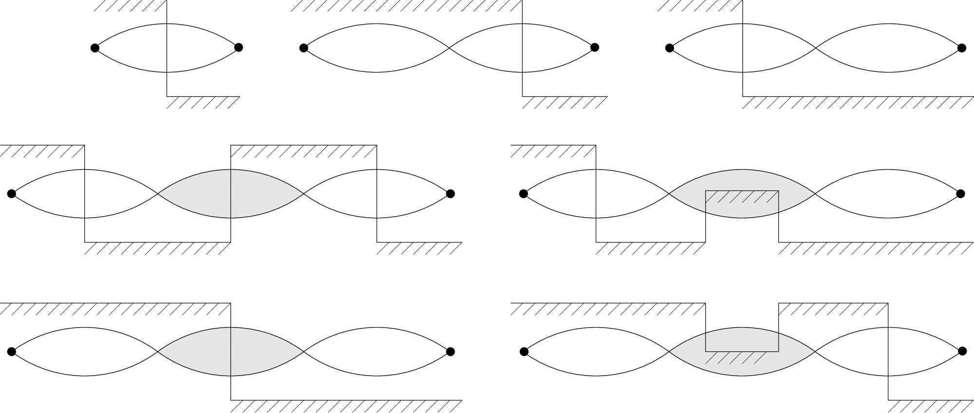
FIG. 34.: Diagrammatic representation of the correlation function $\sigma_{AA}$. Filled bubbles represent the sum of all cut chain diagrams. The external operator $A$ is represented by black circles at each end.

For the sake of simplicity, $\lambda\phi^{4}$ diagrams are examined first. Diagrammatically, the sum of all $\lambda\phi^{4}$ chain diagrams for the Wightman function $\sigma_{AA}^{\vphantom{x}}$ of a bilinear operator $\hat{A}$ can be represented by Fig. 34. The filled bubble in Fig. 34 with the ends of the cut lines on opposite sides represents sum of all cut chain diagrams with the same topology. This sum is denoted by $L_{\rm chain}(q)$. Similarly, the filled bubble with the ends of the cut on the same side represents the sum of all cut diagrams with the equivalent topology. This sum is denoted by $C_{\rm chain}(q)$

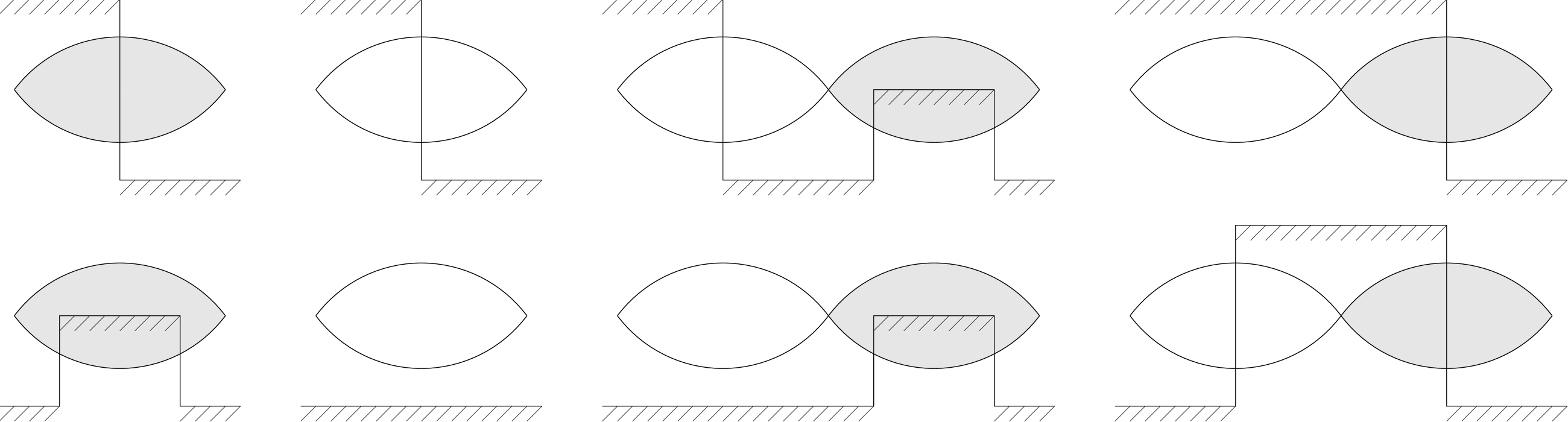
FIG. 35.: Diagrammatic representation of the equations satisfied by the resummed cut and uncut bubbles. In this diagram, the external operators at both ends are $\hat{\phi}^{2}$ rather than $\hat{A}$. The sum of all chain diagrams for correlation function $\sigma_{AA}$ can be expressed in terms of the solutions of these equations. The empty cut bubble is denoted by $L(q)$, the empty uncut bubble $C(q)$. The filled bubble on the left hand side of the first diagram is denoted by $L_{\rm chain}(q)$, the filled bubble on the right hand side of the second diagram is $C_{\rm chain}(q)$.

The equations for $L_{\rm chain}(q)$ and $C_{\rm chain}(q)$ are

$$\left(\begin{array}[]{l}L_{\rm chain}(q)\\ C_{\rm chain}(q)\end{array}\right)=\left(\begin{array}[]{l}L_{0}(q)\\ C_{0}(q)\end{array}\right)+\lambda\left(\begin{array}[]{ll}C_{0}(q)^{*}&L_{0}(q)\\ L_{0}(-q)&C_{0}(q)\end{array}\right)\left(\begin{array}[]{l}L_{\rm chain}(q)\\ C_{\rm chain}(q)\end{array}\right)\;,$$ (F1)

as illustrated in Fig. 35. The cut bubble $L_{0}(q)$ and the uncut bubble $C_{0}(q)$ are again defined by Eq. (59) and Eq. (60) with $I_{A}(l,q{-}l)=1$.

The above matrix equation is easy to solve. The solution is

$$L_{\rm chain}(q) = \displaystyle{L_{0}(q)\over(1-\lambda{\rm Re}\,C(q))^{2}+({\textstyle{\lambda\over 2}})^{2}(L(q)-L(-q))^{2}}\;$$ (F3)

and

$$C_{\rm chain}(q) = \displaystyle{C(q)-\lambda(({\rm Re}\,C(q))^{2}-{\textstyle{\lambda\over 4}}(L(q)-L(-q))^{2}\over(1-\lambda{\rm Re}\,C(q))^{2}+({\textstyle{\lambda\over 2}})^{2}(L(q)-L(-q))^{2}}\;,$$ (F4)

where the finite temperature optical theorem

$${\rm Im}\;C(q)=-{1\over 2}\left(L(q)+L(-q)\right)\;,$$ (F5)

is used to obtain the form shown in (F).

When cubic interactions are included, the “chain” diagrams also include cut two-loop diagrams shown in Fig. 9 where the bubble in the diagram may be regarded as the sum of all $\lambda\phi^{4}$ chain diagrams. Equivalently, the vertex contribution may be regarded as containing

$$I_{\tilde{A}}(l,-l)=I_{A}(l,-l)+\lambda{\rm Re}\,C_{A}(0)\times\left(1+{\cal O}(\sqrt{\lambda})\right)\;.$$ (F6)

A straight forward application of cutting rules then yields,

$$\sigma_{AA}^{\hbox{{Fig.~{}{\ref{fig:chain3}}}}}(0) = \displaystyle-4iL_{\tilde{A}}(0)\,\tilde{G}(0)\,C_{\tilde{A}}(0)+4iC_{\tilde{A}}(0)^{*}\,\tilde{G}(0)^{*}\,L_{\tilde{A}}(0)$$ (F8)

$$\displaystyle{}+4C_{\tilde{A}}(0)^{*}\,S(0)\,C_{\tilde{A}}(0)+4L_{\tilde{A}}(0)\,S(0)\,L_{\tilde{A}}(0)$$

$$= \displaystyle-8{g^{2}\over m_{\rm th}^{2}}\,{\rm Re}\,C_{\tilde{A}}(0)L_{\tilde{A}}(0)+4{g^{4}\over m_{\rm th}^{4}}\,\left({\rm Re}\,C_{\tilde{A}}(0)\right)^{2}L_{0}(0)\;,$$ (F9)

where the optical theorem (69), and $S(0)=g^{2}L_{0}(0)/m_{\rm th}^{4}$, justified below, are used.

For the remainder of this appendix, the estimates ${\rm Re}\,C_{A}(0)={\cal O}(T^{2})$, ${\rm Re}\,C_{0}(0)={\cal O}(1/\sqrt{\lambda})$, $g^{2}\tilde{G}(0)={\cal O}(g^{2}/m_{\rm th}^{2})$, and $S(0)={\cal O}(1/\lambda^{2}T^{2})$ used in this appendix and section III D are examined. To estimate ${\rm Re}\,C_{A}(0)$, consider the following explicit form of the real part of an uncut bubble $C_{A}(0)$

$${\rm Re}\,C_{A}(0) = \displaystyle{1\over 2}\int{d^{4}l\over(2\pi)^{4}}\,I_{A}(l,-l)\,{\rm Re}\,(-i\tilde{G}^{2}(l))\,$$ (F10)

$$= \displaystyle{i\over 4}\int{d^{4}l\over(2\pi)^{4}}\,I_{A}(l,-l)\,\coth(l^{0}\beta/2)\,\left({1\over[l^{2}+m_{\rm th}^{2}+\Sigma(l)]^{2}}-{1\over[l^{2}+m_{\rm th}^{2}+\Sigma(l)^{*}]^{2}}\right)$$ (F11)

$$= \displaystyle{1\over 4}\left.{\partial\over\partial m^{2}}\int{d^{4}l\over(2\pi)^{4}}\,I_{A}(l,-l)\,\coth(|l^{0}|\beta/2)\,2\pi\delta(l^{2}+m^{2})\right|_{m^{2}=m_{\rm th}^{2}}\times(1+{\cal O}(\lambda^{2}))\;,$$ (F12)

where to obtain the last line, the elementary relation

$${\partial\over\partial x}\left({1\over x+a}\right)=-{1\over(x+a)^{2}}\;,$$ (F13)

and the single particle spectral density in the weak coupling limit,

$$\rho(l) = \displaystyle{i\over[l^{2}+m_{\rm th}^{2}+\Sigma(l)]}-{i\over[l^{2}+m_{\rm th}^{2}+\Sigma(l)^{*}]}$$ (F14)

$$= \displaystyle\rho_{\rm free}(l)\,\times(1+{\cal O}(\lambda^{2}))\;,$$ (F15)

are used. Note that the identification $m^{2}=m_{\rm th}^{2}$ must be made after the derivative is taken. Again at high temperature, the zero temperature contribution is smaller than the thermal contribution. Hence, the $\coth(\beta E_{l}/2)$ factor in the integrand can be replaced by the Bose factor $2n(E_{l})$ to calculate the leading weak coupling behavior.

For the pressure and the energy density insertions,

$${\rm Re}\,C_{\cal P}(0) = \displaystyle{1\over 2}\left.{\partial\over\partial m^{2}}\int{d^{3}{\bf l}\over(2\pi)^{3}E_{l}}\,n(E_{l})\,{\textstyle{1\over 3}}{\bf l}^{2}\,\right|_{m^{2}=m_{\rm th}^{2}}$$ (F16)

$$= \displaystyle{1\over 2}\left.{\partial\over\partial m^{2}}{\cal P}_{0}\right|_{m^{2}=m_{\rm th}^{2}}=-{T^{2}\over 48}\;,$$ (F17)

and

$${\rm Re}\,C_{\varepsilon}(0) = \displaystyle{1\over 2}\left.{\partial\over\partial m^{2}}\int{d^{3}{\bf l}\over(2\pi)^{3}E_{l}}\,n(E_{l})\,E_{l}^{2}\,\right|_{m^{2}=m_{\rm th}^{2}}$$ (F18)

$$= \displaystyle{1\over 2}\left.{\partial\over\partial m^{2}}\left(3{\cal P}_{0}{+}{m^{2}T^{2}\over 12}\right)\right|_{m^{2}=m_{\rm th}^{2}}=-{T^{2}\over 48}\;,$$ (F19)

ignoring higher order contributions.

The expression for ${\rm Re}\,C_{0}(0)$ is also given by Eq. (64) by setting $I_{A}=1$. At high temperature, the leading ${\cal O}(T^{2})$ contribution to the integral in the last expression in Eq. (64) comes from loop momenta of ${\cal O}(T)$. However, when the derivative with respect to $m^{2}$ is taken, this is zero. The next largest contribution to the integral is ${\cal O}(mT)$ coming from loop momenta of ${\cal O}(m)$. When the mass derivative is taken and the identification $m\to m_{\rm th}$ made, this yields ${\rm Re}\,C_{0}(0)={\cal O}(T/m_{\rm th})={\cal O}(1/\sqrt{\lambda})$.

To estimate the size of propagators at zero momentum requires knowledge of the size of the self-energy at zero external momentum. The lowest order imaginary part of the off-shell self-energy comes from the $g\phi^{3}$ one-loop diagram shown in Fig. 2. To estimate the size of this diagram, the propagators in the loop must be regarded as resummed propagators. Then the self-energy in the zero 4-momentum limit satisfies

$$\lim_{q^{0}\to 0}\,\lim_{{\bf q}\to 0}\,2[1{+}n(q^{0})]\,\Sigma_{I}(q) = \displaystyle g^{2}\,L_{0}(0)\times(1+{\cal O}(\lambda))$$ (F20)

$$= \displaystyle{\cal O}(g^{2}/\lambda^{2})={\cal O}(m_{\rm phys}^{2}/\lambda)\;,$$ (F21)

where pinching pole approximation of $L(0)$ is again used. The above estimate for the self-energy implies that,

$$\lim_{q^{0}\to 0}\,\lim_{{\bf q}\to 0}\,S(q) = \displaystyle\lim_{q^{0}\to 0}\,\lim_{{\bf q}\to 0}\,{2[1{+}n(q^{0})]\Sigma_{I}(q)\over|q^{2}+m_{\rm th}^{2}+\Sigma(q)|^{2}}$$ (F22)

$$= \displaystyle{g^{2}L_{0}(0)\over m_{\rm th}^{4}}\times(1+{\cal O}(\sqrt{\lambda}))$$ (F23)

$$= \displaystyle{\cal O}(g^{2}/\lambda^{4}T^{4})={\cal O}(m_{\rm phys}^{2}/\lambda^{3}T^{4})$$ (F24)

$$= \displaystyle{\cal O}(1/\lambda^{3}T^{2}\times(g^{2}/T^{2}))\leq{\cal O}(1/\lambda^{2}T^{2})\;,$$ (F25)

and

$$\lim_{q^{0}\to 0}\,\lim_{{\bf q}\to 0}\,g^{2}\,{\rm Re}\,\tilde{G}(q) = \displaystyle\lim_{q^{0}\to 0}\,\lim_{{\bf q}\to 0}\,{g^{2}\,[q^{2}+m_{\rm th}^{2}+\Sigma_{R}(q)]\over|q^{2}+m_{\rm th}^{2}+\Sigma(q)|^{2}}$$ (F26)

$$= \displaystyle{\cal O}(g^{2}/m_{\rm th}^{2})={\cal O}(\lambda m_{\rm phys}^{2}/m_{\rm th}^{2})\leq{\cal O}(\lambda)\;.$$ (F27)

G The imaginary part of two-loop self-energy

Using the cutting rules, the imaginary part of the two-loop self-energy can be expressed as

$$\Sigma_{I}^{\hbox{{two-loop}}}(\underline{q})\equiv{\lambda^{2}\over 12}(1{-}e^{-\beta E_{q}})\,{\cal S}(\underline{q})\;,$$ (G1)

where

$${\cal S}(\underline{q})\equiv\int{d^{4}l\over(2\pi)^{4}}\,{d^{4}k\over(2\pi)^{4}}\,S_{\rm free}(l)\,S_{\rm free}(k{+}\underline{q})\,S_{\rm free}(-l{-}k)\,\;.$$ (G2)

Using the on-shell $\delta$-functions free particle cut propagators

$$S_{\rm free}(l)=\sum_{\sigma_{l}=\pm 1}\,\sigma_{l}\,[1{+}n(\sigma_{l}E_{l})]\,\pi\delta(l^{0}-\sigma_{l}E_{l}){\bigg{/}}E_{l}\;,$$ (G3)

frequency integrations in Eq. (G2) can be straightforwardly carried out to yield

$${\cal S}(\underline{q}) \displaystyle= \displaystyle\sum_{\sigma=\pm 1}\,\sigma_{k+q}\sigma_{l+k}\sigma_{l}{1\over 8(2\pi)^{5}}\int{d^{3}{\bf l}\,d^{3}{\bf k}\over E_{l}E_{k+q}E_{k+l}}\,[1{+}n(\sigma_{k+q}E_{k+q})]\,[1{+}n(\sigma_{l}E_{l})]\,$$ (G5)

$$\displaystyle\quad\quad{}\times[1{+}n(\sigma_{k+l}E_{k+l})]\,\delta(E_{q}{-}\sigma_{l}E_{l}{-}\sigma_{k+q}E_{k+q}{-}\sigma_{k+l}E_{k+l})\,\;.$$

The argument of remaining $\delta$-function can be satisfied only when two of the $\sigma$ are $+1$ and the other one is $-1$. By suitably changing labels, the above then becomes

$${\cal S}(\underline{q})={3\over 8(2\pi)^{5}}\int{d^{3}{\bf l}\,d^{3}{\bf k}\over E_{l}E_{k+q}E_{k+l}}\,[1{+}n(E_{l})]\,[1{+}n(E_{k+q})]\,n(E_{k+l})\,\delta(E_{q}{+}E_{k+l}{-}E_{k+q}{-}E_{l})\,\;.$$ (G6)

To carry out remaining integrations, the angles between spatial vectors are defined as

$$\cos\theta_{k} \displaystyle\equiv \displaystyle{{\bf k}{\cdot}{\bf q}/|{\bf k}||{\bf q}|}$$ (G7)

$$\cos\theta_{l} \displaystyle\equiv \displaystyle{{\bf k}{\cdot}{\bf l}/|{\bf k}||{\bf l}|}\;.$$ (G8)

Changing variables to $E_{k+q}$ and $E_{k+l}$ with the Jacobians

$${dE_{k+q}/d\cos\theta_{k}} \displaystyle= \displaystyle{|{\bf k}||{\bf q}|/E_{k+q}}$$ (G9)

$${dE_{k+l}/d\cos\theta_{l}} \displaystyle= \displaystyle{|{\bf k}||{\bf l}|/E_{k+l}}\;,$$ (G10)

one finds

$${\cal S}(\underline{q}) \displaystyle= \displaystyle{3\over 8(2\pi)^{5}|{\bf q}|}\int dE_{l}\,d|{\bf k}|\,[1{+}n(E_{l})]\,\int_{E^{-}_{kl}}^{E^{+}_{kl}}dE_{k+l}\,\int_{E^{-}_{kq}}^{E^{+}_{kq}}dE_{k+q}\,[1{+}n(E_{k+q})]\,$$ (G12)

$$\displaystyle\quad\quad{}\times n(E_{k+l})\,\delta(E_{q}{+}E_{k+l}{-}E_{k+q}{-}E_{l})\,\;,$$

where

$$E^{\pm}_{kl}\equiv\sqrt{(|{\bf k}|{\pm}|{\bf l}|)^{2}+m_{\rm th}^{2}}\;,$$ (G13)

with analogous definitions for $E^{\pm}_{kq}$. Carrying $E_{k+q}$ and $E_{k+l}$ integrations amounts to figuring out the kinematic conditions. Straightforward calculation then yields

$${\cal S}(\underline{q})={3T\over 32\pi^{3}|{\bf q}|}\int_{0}^{|{\bf q}|}d|{\bf k}|\,$$ (G16)

$$\displaystyle\quad{}\times\left\{\int_{E_{k}}^{E_{q}}dE_{l}\,[1{+}n(E_{l})][1{+}n(E_{q}{-}E_{l})]\,\ln\left(e^{-\beta E_{l}}{-}e^{-\beta(E_{q}{+}E_{k})}\over e^{-\beta E_{l}}(1{-}e^{-\beta E_{k}})\right)\right.$$

$$\displaystyle\quad\;\;{}+\left.\int_{E_{q}}^{\infty}dE_{l}\,[1{+}n(E_{l})][1{+}n(E_{q}{-}E_{l})]\,\ln\left(e^{-\beta E_{q}}(1{-}e^{-\beta E_{k}})\over e^{-\beta E_{q}}{-}e^{-\beta(E_{l}{+}E_{k})}\right)\right\}\;.$$

Changing variables from $E_{l}$ to $u\equiv e^{-\beta E_{l}}$, the above can be rewritten as

$${\cal S}(\underline{q})={3T^{2}\over 32\pi^{3}|{\bf q}|}[1{+}n(E_{q})]\int_{0}^{|{\bf q}|}d|{\bf k}|\,$$ (G19)

$$\displaystyle\quad{}\times\left\{\int_{y}^{x}du\,\left({1\over 1{-}u}+{1\over u{-}y}\right)\ln\left({u{-}yx\over u(1{-}x)}\right)\right.$$

$$\displaystyle\quad\;\;{}+\left.\int_{0}^{y}du\,\left({1\over 1{-}u}+{1\over u{-}y}\right)\ln\left({y(1{-}x)\over y{-}ux}\right)\right\}\;,$$

where

$$y \displaystyle\equiv \displaystyle e^{-\beta E_{q}}\;,$$ (G20)

$$x \displaystyle\equiv \displaystyle e^{-\beta E_{k}}\;.$$ (G21)

Another change of variable

$$z\equiv{u{-}y\over 1{-}u}\;,$$ (G22)

and the definition of dilogarithmic function,

$$Li_{2}(z)\equiv-\int_{0}^{1}{du\over u}\,\ln(1{-}zu)=\sum_{n=1}^{\infty}\,{z^{n}\over n^{2}}\;,$$ (G23)

yield,

$${\cal S}(\underline{q})={3T^{2}\over 32\pi^{3}|{\bf q}|}\,[1{+}n(E_{q})]\int_{0}^{|{\bf q}|}d|{\bf k}|\,$$ (G26)

$$\displaystyle\quad{}\times\left(\ln\left({x\over y}\right)\,\ln\left({1{-}y\over 1{-}x}\right)\,+2\ln^{2}\left({1{-}y\over 1{-}x}\right)\,\right.$$

$$\displaystyle\quad{}\left.+Li_{2}(y)+Li_{2}\left({(1{-}xy)(x{-}y)\over x(1{-}y)^{2}}\right)+Li_{2}\left({x{-}y\over 1{-}y}\right)-Li_{2}\left({x{-}y\over x(1{-}y)}\right)\right)\;.$$

In the $|{\bf q}|\to 0$ limit, $x=y$. Hence, immediately,

$${\cal S}(m_{\rm th},0)={3T^{2}\over 32\pi^{3}}\,[1{+}n(m_{\rm th})]\,Li_{2}(e^{-\beta m_{\rm th}})\;,$$ (G27)

and

$$\Sigma_{I}^{\hbox{{two-loop}}}(m_{\rm th},0)={\lambda^{2}T^{2}\over 2^{7}\pi^{3}}\,Li_{2}(e^{-\beta m_{\rm th}})\;.$$ (G28)

When the temperature is high, $T\gg m_{\rm th}$, the identity

$$Li_{2}(x)={\pi^{2}\over 6}-\ln(x)\ln(1{-}x)-Li_{2}(1{-}x)\;,$$ (G29)

yield

$$\Sigma_{I}^{\hbox{{two-loop}}}(m_{\rm th},0)={T^{2}\lambda^{2}\over 768\pi}(1+{\cal O}(m_{\rm th}/T\ln(m_{\rm th}/T)))\;.$$ (G30)

When the temperature is low, $T\ll m_{\rm th}$, the dilogarithmic function $Li_{2}(e^{-\beta m_{\rm th}})=e^{-m_{\rm th}\beta}$, and

$$\Sigma_{I}^{\hbox{{two-loop}}}(m_{\rm th},0)={\lambda^{2}T^{2}\over 128\pi}\,e^{-m_{\rm th}\beta}\,\times(1+{\cal O}(e^{-m_{\rm th}\beta}))\;.$$ (G31)

In the opposite limit where $|{\bf q}|\to\infty$, the only term that survives in ${\cal S}$ is the first term in the bracket

$$\lim_{q\to\infty}{\cal S}(\underline{q})=-{3T^{2}\over 32\pi^{3}}\,\int_{0}^{\infty}d|{\bf k}|\,\ln(1{-}e^{-\beta E_{k}})\;.$$ (G32)

In the high temperature limit, this yields

$$\lim_{q\to\infty}{\cal S}(\underline{q}) \displaystyle= \displaystyle{3T^{2}\over 32\pi^{3}}\,\left({\pi^{2}\over 6}+{\cal O}(m_{\rm th}^{2}/T^{2})\right)\;,$$ (G33)

and

$$\lim_{q\to\infty}\Sigma_{I}^{\hbox{{two-loop}}}(\underline{q}) \displaystyle= \displaystyle{T^{2}\lambda^{2}\over 768\pi}(1+{\cal O}(m_{\rm th}^{2}/T^{2}))\;.$$ (G34)

Note that the leading order terms are the same. In the low temperature limit,

$$\lim_{q\to\infty}\Sigma_{I}^{\hbox{{two-loop}}}(\underline{q})={\lambda^{2}\over 128\pi}\,e^{-m_{\rm th}\beta}\,\sqrt{m_{\rm th}T^{3}\over 2\pi^{3}}\,\times(1+{\cal O}(e^{-m_{\rm th}\beta}))\;.$$ (G35)

FIG. 36.: Numerical results for $\tilde{\Sigma}_{I}(E_{k})=768\pi\Sigma_{I}(E_{k})/\lambda^{2}T^{2}$ for $m_{\rm th}/T=0.01,0.1$.

FIG. 37.: $\tilde{\Sigma}_{I}(E_{k})=768\pi\Sigma_{I}(E_{k})/\lambda^{2}T^{2}$ with $m_{\rm th}/T=0.01,0.1$ for small values of $|{\bf k}|/T$.

Numerical integration results shown in Fig. 36 confirms this. A closer look at $\Sigma_{I}(\underline{q})$ with $m_{\rm th}/T=0.01,0.1$ for small values of $|{\bf k}|/T$ is presented in Fig. 37, and $\Sigma_{I}(\underline{q})$ for $m_{\rm th}/T=1.0,2.0,3.0$ is given in Fig. 38. Note that as the mass increases, the self-energy becomes flat throughout the momentum range.

FIG. 38.: Numerical results for $\tilde{\Sigma}_{I}(E_{k})=768\pi\Sigma_{I}(E_{k})/\lambda^{2}T^{2}$ for $m_{\rm th}/T=1.0,2.0,3.0$.

REFERENCES

• [1] L.P. Kadanoff and P.C. Martin, Hydrodynamic Equations and Correlation Functions, Ann. Phys. (NY) 24, 419, (1963).
• [2] A. Hosoya, M. Sakagami, and M. Takao, Non-equilibrium Thermodynamics in Field Theory: Transport Coefficients, Ann. of Phys. (NY) 154, 229 (1984) and references therein.
• [3] R. Horsley and W. Schoenmaker, Quantum Field Theories out of Thermal Equilibrium (1), Nuc. Phys. B 280, 716 (1987).
• [4] For example, see G.D. Mahan, Many-Particle Physics, Plenum Press, New York (1981).
• [5] S. Jeon, Computing Spectral Densities in Finite Temperature Field Theory, Phys. Rev. D 47, 4568 (1993).
• [6] For example, see L.D. Landau and E.M. Lifshitz, Fluid Mechanics, Pergamon Press, (1959).
• [7] E. Calzetta and B.L. Hu, Nonequilibrium Quantum Fields: Closed-Time-Path Effective Action, Wigner Function, and Boltzmann Equation, Phys. Rev. D 37, 2878, (1988).
• [8] D. Forster, Hydrodynamic Fluctuations, Broken Symmetry, and Correlation Functions, Addison-Wesley Publishing Company, Inc. (1975).
• [9] S. Weinberg, Gravitation and Cosmology, John Wiley and Sons, (1972).
• [10] For example, see H. Smith and H.H. Jensen, Transport Phenomena, Oxford University Press, (1989).
• [11] Private communications.
• [12] For example, see A.L. Fetter and J.D. Walecka, Quantum Theory of Many Particle systems, McGraw Hill (1971).
• [13] For example, see L.S. Brown, Quantum Field Theory, Cambridge University Press (1992).
• [14] S. Coleman and R.E. Norton, Singularities in the Physical Region, Nuovo Cimento 38, 438 (1965).
• [15] R.L. Kobes and G.W. Semenoff, Discontinuity of Green Functions in Field Theory at Finite Temperature and Density (II), Nuc. Phys. B 272, 329, (1986).
• [16] For example, see P. Roman, Introduction to Quantum Field Theory, John Wiley and Sons, (1969).
• [17] For example, see J.D. Bjorken and S.D. Drell, Relativistic Quantum Fields, McGraw Hill, (1965).
• [18] L.S. Brown, Dimensional Regularization of Composite Operators in Scalar Field Theory, Ann. Phys. (NY) 126, 135, (1980).
• [19] S.R. de Groot, W.A. van Leeuwen, and Ch.G. van Weert, Relativistic Kinetic Theory, North-Holland Publishing Company (1980) and references therein.
• [20] For example, see W.H. Press, B.P. Flannery, S.A. Teukolsky, W.T. Vetterling, Numerical Recipes in C, Cambridge University Press, (1988).
• [21] For example, see J.I. Kapusta, Finite Temperature Field Theory, Cambridge University Press (1989) and the references therein.
• [22] For example, see D.J. Gross, R.D. Pisarski, L.G. Yaffe, QCD and Instantons at Finite Temperature, Rev. Mod. Phys. 53, 43, (1981).
• [23] For example, see I.S. Gradshteyn and I.M. Ryzhik, Tables of Integrals, Series, and Products, Academic Press, (1980).
• [24] R.R. Parwani, Resummation in a Hot Scalar Field Theory, Phys. Rev. D 45, 4695, (1992).