UFTP preprint 366/1994

QCD Sum Rule Calculation of Twist-3 Contributions to Polarized Nucleon Structure Functions

E. Stein¹, P. Górnicki², L. Mankiewicz³, A. Schäfer¹ and W. Greiner¹

¹Institut für Theoretische Physik, J. W. Goethe Universität Frankfurt,

Postfach 11 19 32, W-60054 Frankfurt am Main, Germany

²Institute of Physics, Polish Academy of Sciences, Al. Lotnikow 32/46, PL-02-668 Warsaw, Poland

³N. Copernicus Astronomical Center, Bartycka 18, PL–00–716 Warsaw, Poland

Abstract:

Using the framework of QCD sum rules we predict the twist-3 contribution to the second moment of the polarized nucleon structure function $g_{2}(x)$. As the relevant local operator depends explicitely on the gluon field, we employ a recently studied interpolating nucleon current which contains three quark field and one gluon field operator. Despite the fact that our calculation is based on the analysis of a completely different correlation function, our estimates are consitent with those of Balitsky, Braun and Kolesnichenko who used a three-quark current.

Considerable attention has been paid to measurements of the polarized structure function $g_{1}$ in deep inelastic scattering. The unexpected EMC [1] results for the first moment of $g_{1}^{p}$, the structure function of the proton, invoked tremendous effort to gain more knowledge about polarized scattering. As a result of these intense discussions it became clear that polarization phenomena might offer much better opportunities to test QCD than unpolarized experiments. Meanwhile SMC [2] and SLAC [3] experiments have provided date on $g_{1}^{n}$ and much improved ones on $g_{1}^{p}$. Mainly due to this experiments the general interest shifted to related questions most notably to the problem of $Q^{2}$ dependence. It turned out that an estimate of the magnitude of higher twist contributions is urgently needed in order to compare the experiments of SLAC, SMC and EMC which cover different $Q^{2}$ regions [4]. This is especially important for the SLAC data which correspond to $Q^{2}$ around 2 ${\rm GeV^{2}}$. Besides being of great importance for the interpretation of the experiments it became also clear that the leading higher matrix elements test fundamental properties of the nucleon. Most notably $d^{(2)}$ on which we will focus in this contribution is a measure for the mean colour-magnetic field in the direction of a transverse nucleon spin. (Due to colour symmetry the expectation value $\langle\vec{B}^{a}\rangle=0$, but the expectation value of the colour singlet $\langle\bar{q}B_{1}q\rangle=\langle\bar{q}\gamma_{0}\tilde{G}_{01}q\rangle\sim d^{(2)}$ can be nonzero.)

The first moment of $g_{1}(x,Q^{2})$ at fixed $Q^{2}$ is given by [5]

$$\int_{0}^{1}dx\;g_{1}(x,Q^{2})=\frac{1}{2}a^{(0)}+\frac{m_{N}^{2}}{9Q^{2}}\left(a^{(2)}+4d^{(2)}+4f^{(2)}\right)+O(\frac{m_{N}^{4}}{Q^{4}})\;.$$ (1)

The above formula does not include perturbative corrections (QCD). Higher order corrections were recently calculated in the leading twist approximation up to $O(\alpha_{S}^{3})$ for non-singlet quantities, the Bjorken sum rule and – up to $O(\alpha_{S}^{2})$ – for the Ellis-Jaffe sum rule [6]. The Ellis-Jaffe sum rule has a flavour singlet contribution.

The reduced matrix elements for the twist-3 and twist-4 components of Eq. (1) are defined by:

$$\frac{1}{6}\langle pS|\bar{q}(0)\left[\gamma^{\alpha}g\tilde{G}^{\beta\sigma}+\gamma^{\beta}g\tilde{G}^{\alpha\sigma}\right]q(0)|pS\rangle-{\rm traces}=$$

$$=2d^{(2)}\left[\frac{1}{6}\left(2p^{\alpha}p^{\beta}S^{\sigma}+2p^{\beta}p^{\alpha}S^{\sigma}-p^{\beta}p^{\sigma}S^{\alpha}-p^{\alpha}p^{\sigma}S^{\beta}-p^{\sigma}p^{\alpha}S^{\beta}-p^{\sigma}p^{\beta}S^{\alpha}\right)\right.$$

$$\enspace-{\rm traces}]\;,$$ (2)

and

$$\langle pS|\bar{q}(0)g\tilde{G}_{\alpha\beta}\gamma^{\beta}q(0)|pS\rangle=2m_{N}^{2}f^{(2)}S_{\alpha}\;$$ (3)

respectively, where $|pS\rangle$ represents the nucleon state of momentum $p$ and spin $S$, $S^{2}=-m_{N}^{2}$.

The $d^{(2)}$ matrix element does not only lead to a contribution to the Ellis-Jaffe and Bjorken sum rules but is also in principle measureable as the twist-3 contribution to the second moment of $g_{2}$ [7]:

$$\int_{0}^{1}dxx^{2}g_{2}(x,Q^{2})=-\frac{2}{3}\int_{0}^{1}dxx^{2}g_{1}(x,Q^{2})+\frac{1}{3}d^{(2)}.$$ (4)

Although both twist-3 and twist-4 matrix elements are interesting, in the present paper we concentrate on the calculation of the twist-3 matrix element $d^{(2)}$ using the QCD sum rules. Some time ago $d^{(2)}$ and $f^{(2)}$ were estimated with this technique by Balitsky, Braun and Kolesnichenko (BBK) [8]. They got rather suprising results, namely a strong asymmetry between $d^{(2)}_{\rm BBK}({\rm proton})$ and $d^{(2)}_{\rm BBK}({\rm neutron})$ and a $d^{(2)}_{\rm BBK}({\rm proton})$ which has opposite sign to that suggested by bag model calculations. [9]. It has been argued [10] that these qualitative properties should be observable in other spin-dependent effects, like single spin asymmetries, such that their unambigious determination is of great importance. Any calculation of a non-perturbative quantity like $d^{(2)}$ has to be based on a trustworthy well definded method which is insensitive to technical details and physicaly irrelevant assumptions. In our opinion the only such available techniques are QCD sum rules and lattice gauge calculations. The latter are tried but are still in prelimenary state. [11]. Thus the reliability of the BBK result can only be checked by consistency tests, namley by comparing the results of calculations with substantially different interpolating currents for which the systematic errors are uncorrelated. The spread of obtained results gives a good estimate for the size of the systematic errors involved. There is actually reason for concern. The chiral structure of the three-quark current used by BBK is such, that graphs of a certain topology “accidentally” vanish because a trace of an odd number of gamma-matrices has to be taken. Unfortunately their sum rule is primarily determined by just a single graph and for this graph the up-quark contribution vanishes due to the special structure of the used three-quark current. Therefore the question arises if the obtained result reflects only the the symmetry of the choosen current or if there is some deeper physical reason behind this. In this situation independent tests with different (more complicated) interpolating nucleon fields are obviously necessary.

Unluckily the QCD sum rules technique used to estimate the matrix elements present in Eqs. (S0.Ex1) and (3) leads to very complex computations. As the consequence the fundamental results of BBK have not yet been checked. Given their importance for the phenomenology we have decided to meet the challenge and to perform an independent calculation with a different interpolating current for the nucleon.

The starting point for calculating the reduced matrix elements of an operator $O_{\Gamma}$ is the three-point correlation function

$$\Pi_{\Gamma}(p)=i^{2}\int d^{4}xe^{ipx}\int d^{4}y\langle 0|T\left\{\eta(x)O_{\Gamma}(y)\overline{\eta}(0)\right\}|0\rangle$$ (5)

where $\eta(x)$, $\langle 0|\eta(0)|pS\rangle=\lambda u(p,S)$ is an interpolating current for the nucleon. There exists a certain freedom of choice for this current. While all reasonable choices should give similar results the optimal choice must be tailored to the problem considered. For a long time the standard choice for sum rule calculations of nucleon properties has been the three-quark current introduced by Ioffe [12]

$$\eta_{I}(x)=\left[u^{a}(x)C\gamma_{\mu}u^{b}(x)\right]\gamma_{5}\gamma^{\mu}d^{c}(x)\varepsilon^{abc}.$$ (6)

This current is used by BBK in their calculation.

As it can be seen from (S0.Ex1) and (3), the operators defining $d^{(2)}$ and $f^{(2)}$ explicitely contain the gluonic field operator. This gluonic field has to be matched by another gluonic field operator. Because the three-quark current $\eta_{I}(x)$ does not contain the gluonic operator explicitely the desired contribution must be generated through the perturbative emission of an additional gluon. The amplitude for this process is proportional to the strong coupling constant $g$.

Alternatively, one may consider an interpolating field which in addition to three quark fields contains the gluon field explicitely. In that case gluon emission from the three-quark configuration has a non-perturbative character.

A possible construction of an interpolating current with such properties was discussed in [13]. It was noticed that all the nice features of the current in (6) are preserved by making it nonlocal, e.g. by shifting the $d$-quark to the point $x+\epsilon$ (and adding the required gauge factor to preserve gauge invariance). Expanding two times in $\epsilon$ and averaging over the directions in Euclidean space $\epsilon_{\mu}\epsilon_{\nu}\rightarrow\frac{1}{4}\delta_{\mu\nu}\epsilon^{2}$ one arrives at

$$\eta^{\prime}_{G}(x)=\varepsilon^{abc}(u^{a}(x)C\gamma_{\mu}u^{b}(x))\gamma_{5}\gamma_{\mu}\sigma_{\alpha\beta}\left[{\rm g}G^{\alpha\beta}(x)d(x)\right]^{c}\,.$$ (7)

Finally, projecting out the isospin $\frac{1}{2}$ component leads to the following proton interpolating current:

$$\eta_{G}(x)=\frac{2}{3}\left(\eta^{\rm old}_{G}(x)-\eta^{\rm ex}_{G}(x)\right)\;,$$ (8)

where

$$\eta^{\rm old}_{G}(x)=\varepsilon^{abc}\left(u^{a}(x)C\gamma_{\mu}u^{b}(x)\right)\gamma_{5}\gamma^{\mu}\sigma_{\alpha\beta}\left[G^{\alpha\beta}(x)d(x)\right]^{c}\;,$$ (9)

and

$$\eta^{\rm ex}_{G}(x)=\varepsilon^{abc}\left(u^{a}(x)C\gamma_{\mu}d^{b}(x)\right)\gamma_{5}\gamma^{\mu}\sigma_{\alpha\beta}\left[G^{\alpha\beta}(x)u(x)\right]^{c}\;.$$ (10)

We would like to stress here that the technique of QCD sum rules does not require the use of “the best” current from all the possible ones, it is only necessary that the current is not too bad in order that the contribution of interest is not suppressed by some special reason.

In ref [13] the current (8) was analysed in details and the corresponding overlap $\lambda_{G}$ defined through

$$\langle 0|\eta(0)|pS\rangle=m_{N}^{2}\lambda_{G}u(p,S)\;,$$ (11)

was calculated. Subsequently, it was used to predict the nucleon momentum fraction carried by gluons to be $\sim 0.4$ at $\mu^{2}\sim$ 1 GeV², and the gluon form factor of the proton at $Q^{2}\sim$ 2 – 3 GeV². Both predictions agree very well with present day data and its generally accepted interpretation. This convinced us that the current $\eta_{G}(x)$ is an adequate choice to calculate properties of the nucleon.

From the purely technical point of view the current $\eta_{G}(x)$ differs in one important respect from the Ioffe current $\eta_{I}(x)$. As mentioned before, the chiral structure of $\eta_{I}(x)$ is such that graphs of certain topologies vanish because a trace of an odd numbers of gamma matrices has to be taken. The same happens obviously also for $\eta^{\rm old}(x)$ but from correlators involving $\eta^{\rm ex}(x)$ we obtain non-vanishing contributions form the graphs of the same topology. The calculation is therefore quite different from that described in [8].

It is not yet possible to calculate the three-point correlator defined by Eq. (5) directly. However, the usual philosophy of the QCD sum rules is to relate it to some other correlators using Wilson’s operator product expansion (OPE). As it has been noticed in [14] for the case of a three-point correlation function the expansion is more complicated than in the case of two point functions and has the following structure:

$$\Pi_{\Gamma}(p)=\sum_{n}c_{\Gamma,n}^{\rm L}(p)<O^{\rm L}_{n}>+\sum_{n}c^{\rm BL}_{n}(p)\Pi_{\Gamma,n}^{\rm BL}(0)\;.$$ (12)

As usual the main objective is to separate different scales: vacuum expectation values of local operators $\langle O^{L}\rangle$ and correlators $\Pi^{BL}$ describe long distance effects while the coefficients $c^{L}$ and $c^{BL}$ receive contribution only from highly virtual quark and gluon fields which propagate for small distances. The first part of the expansion – so called local power corrections (LPC) – is well known from two point QCD sum rules. The second part – bilocal power corrections (BPC) – has been introduced in [14] to describe the large $y$ region of the integrand in Eq. (5). This region cannot be properly described by local power corrections alone. Yet, the distinction between large and small distances is somewhat arbitrary and the corresponding scale is implicitly included in the definitions of local and bilocal power corrections. Changing the scale we can shift part of the BPCs to LPCs and vice versa. The optimal scale is always dictated by the nature of the physical phenomena one wants to investigate.

The (OPE) of the correlation function $\Pi_{\Gamma}$ is given by the sum of both LPC’s and BPC’s, as in (12). We note that in general only this sum has a physical meaning and is independent of the regularisation scheme.

The bilocal power corrections are determined by the long-distance, non-perturbative contribution to correlation functions at zero momentum [15]:

$$\Pi_{\Gamma,n}^{\rm BL}(q)=i\int d^{4}ye^{iqy}\langle 0|T\left\{O_{\Gamma}(y)\tilde{O}_{n}(0)\right\}|0\rangle$$ (13)

with $q=0$. The Operators $\tilde{O}_{n}(0)$ are defined by the following series

$$T(\eta_{I}(x){\bar{\eta}}_{G}(0))=\sum_{n}C_{n}^{BL}(x^{2}){\tilde{O}}_{n}(0),$$ (14)

where the above expansion goes over a series of local, gauge-invariant operators of dimension $n$ ${\tilde{O}}_{n}(0)$. When this expansion is inserted back in (5) it gives the second contribution to Eq.(12). We have performed a detailed analysis of the BPC’s to the sum rule for the twist-3 matrix element $d^{(2)}$ and have found that numerically important correlators do not contribute due to symmetry. In this respect the situation is entirely the same as in the case of the calculation discussed in [8].

The QCD sum rules for the twist-3 part of $g_{1}$ can be represented as

$$\frac{1}{4}{\rm Tr}\left[\not\!S\,\gamma_{5}i^{2}\int d^{4}xe^{ipx}\int d^{4}y\langle 0|T\left\{\eta_{I}(x)\bar{q}(y)g\tilde{G}_{\sigma\{\mu}(y)\gamma_{\nu\}}q(y)\eta_{G}(0)\right\}|0\rangle\right]$$

$$=-2\frac{d^{(2)}\lambda_{I}\lambda_{G}S_{[\sigma}p_{\{\mu]}p_{\nu\}}m_{N}^{4}}{(m_{N}^{2}-p^{2})^{2}}+\ldots$$ (15)

$[\ldots]$ means antisymmetrization of the indices, while $\{\ldots\}$ denotes symmetrization resp (see Eq. (S0.Ex1)). Here, we have singled out the double-pole due to the nucleon contribution in the intermediate state; other terms denoted by ellipses at the phenomenological right hand side are less singular in $m_{N}^{2}-p^{2}$ and do not carry any useful information – later on they will be suppressed by suitable treatment. The couplings of the Ioffe current respectively our quark - gluon current to the the nucleon are denoted by $\lambda_{I}$ and $\lambda_{G}$ while $m_{N}$ denotes the nucleon mass.

The left hand side has been expanded and all LPC contributions including operators up to dimension 10 have been calculated. It has required calculation of more than 100 Feynman diagrams. Traces of gamma matrices and other manipulations were done using program TRACER [16] written for MATHEMATICA. Dimensional regularization has been used and the $\gamma_{5}$ matrix has been treated according to the ’t Hooft-Veltman scheme [17].

The result for the twist-3 contribution has the general form

$${\rm Tr}\left[\not\!S\,\gamma_{5}\Pi_{\sigma\mu\nu}(p)\right]=$$

$$\left[A\frac{\alpha_{S}}{\pi^{5}}(-p^{2})^{3}\log(-p^{2}/\mu^{2})+B\frac{\alpha_{S}}{\pi}<\bar{q}q>^{2}\log(-p^{2}/\mu^{2})\right.$$

$$+C\frac{1}{\pi^{4}}<fg^{3}GGG>\log(-p^{2}/\mu^{2})$$

$$+\left(D+F\log(-p^{2}/\mu^{2})\right)\frac{\alpha_{S}}{\pi}\frac{m_{0}^{2}<\bar{q}q>^{2}}{-p^{2}}$$

$$\left.+G\frac{<\bar{q}q>^{2}<g^{2}G^{2}>}{(-p^{2})^{2}}+H\frac{<\bar{q}q>^{2}m_{0}^{4}}{(-p^{2})^{2}}\right]S_{[\sigma}p_{\{\mu]}p_{\nu\}}$$ (16)

where the numerical coefficients are given in Table 1. Note that the coefficient in front of the gluon condensate $\langle GG\rangle$ vanishes.

	$A$	$B$	$C$	$D$	$F$	$G$	$H$
d	$1/(3^{4}2^{7})$	8/27	$1/(3^{2}2^{6})$	85/162	-95/648	10/81	2/9
u	$1/(3^{4}2^{6})$	4/9	$1/(3^{2}2^{5})$	-847/2592	-13/324	2/81	-1/27

Table 1: Numerical coefficients corresponding to the sum rule eq. S0.Ex4. The upper line gives the values for the twist-3 operator involving d quarks, the lower line for the corresponding operator with u-quarks

There are two types of unwanted terms at the phenomenological sides of the sum rules. The first type are the terms containing a $(m_{N}^{2}-p^{2})^{-1}$ singularity. The second are pure continuum contributions which correspond to contributions from various higher resonances etc. To deal with these terms we first multiply both sides of the sum rules by $(m_{N}^{2}-p^{2})$ and then perform the Borel transform and a suitable continuum subtraction. The multiplication has a twofold effect: (a) it lowers the singularity of the first term and (b) removes the $m_{N}^{2}-p^{2}$ singularities from all other terms. In that way the only low lying singularity is that of the first term. The singularities at higher values of $-p^{2}$ are suppressed by the Borel transformation. The transformed sum rule for twist-3 contribution looks as follows:

$$-16d^{(2)}\lambda_{I}\lambda_{G}m_{N}^{4}e^{-m_{N}^{2}/M^{2}}$$

$$=3!M^{12}\tilde{A}(\frac{m_{N}^{2}}{M^{2}}E_{4}-4E_{5})+M^{6}(\tilde{B}+\tilde{C})(E_{2}-\frac{m_{N}^{2}}{M^{2}}E_{1})+M^{2}m_{N}^{2}\tilde{D}+$$

$$M^{4}\tilde{F}(\frac{m_{N}^{2}}{M^{2}}\log(M^{2}/\mu^{2})-E_{1})+M^{2}(\tilde{G}+\tilde{H})(\frac{m_{N}^{2}}{M^{2}}+1)$$ (17)

where

$$E_{n}=1-e^{\left(-s_{0}/M^{2}\right)}\sum_{k=0}^{n-1}\frac{1}{k!}\left(s_{0}/M^{2}\right)^{k}$$ (18)

Here we absorbed the condensates, $\alpha_{S}$ and $\pi$ factors in the definition of the coefficients $\tilde{A},\tilde{B},\ldots$ which then are given by $\tilde{A}=\alpha_{S}A/\pi^{5}$, $\tilde{B}=\alpha_{S}<\bar{q}q>^{2}B/\pi$, $\tilde{C}=<fg^{3}GGG>C/\pi^{4}$, $\tilde{D}=\alpha_{S}m_{0}^{2}<\bar{q}q>^{2}D/\pi$, $\tilde{F}=\alpha_{S}m_{0}^{2}<\bar{q}q>^{2}F/\pi$, $\tilde{G}=<g^{2}G^{2}><\bar{q}q>^{2}G$, $\tilde{H}=m_{0}^{4}<\bar{q}q>^{2}H$.
One point requires explanation here. The term associated with the dimension-8 condensate in the sum rule for the matrix element of the twist-3 operator contains arbitrary scale $\mu$ even after Borel transformation. This dependence may be traced back to the occurence of terms proportional to $\log(-p^{2}/\mu^{2})/p^{2}$ in the original sum rule. They arise because of the mixing of the three-point correlation function (5) with two-point correlation functions of the nucleon currents $\eta_{I}(x)$ and ${\bar{\eta}}_{G}(0)$ with operators produced by the contraction of $O_{\Gamma}(y)$ with ${\bar{\eta}}_{G}(0)$ and $\eta_{I}(x)$, respectively [18]. The natural choice of the scale is $\mu\approx$ 1 GeV which corresponds to the typical values of momenta in the intermediate region where the sum rule equality is expected to hold. Fortunately the numerical coefficient associated with this term is small.

The condensates have been normalized at 1 GeV. Their values: $<\bar{q}q>=(-0.257{\rm GeV})^{3}$, $<\alpha_{s}/\pi GG>=0.012{\rm GeV}^{4}$, $m_{0}^{2}=<\bar{q}g\sigma Gq>/<\bar{q}q>=0.65{\rm GeV^{2}}$ and $<fg^{3}GGG>=0.046{\rm GeV^{6}}$ correspond to the standard ITEP values rescaled to the normalization point $\mu^{2}\sim m_{N}^{2}\sim 1\;{\rm GeV^{2}}$. The strong coupling at $1\;{\rm GeV}$ is taken to be $\alpha_{S}=0.37$ ($\Lambda=150)$ MeV. The continuum threshold is taken at $s_{0}=(1.5{\rm GeV})^{2}$ roughly corresponding to the Roper resonance position.

The coupling constants $\lambda_{I}$ and $\lambda_{G}$ may be calculated from the two point sum rule derived in [13]

$$2(2\pi)^{4}m_{N}^{2}\lambda_{I}\lambda_{G}e^{-m_{N}^{2}/M^{2}}=\frac{6}{5}\frac{\alpha_{S}}{\pi}M^{8}E_{4}$$

$$+\frac{1}{2}<g^{2}GG>M^{4}E_{2}-\frac{4}{3}\frac{\alpha_{s}}{\pi}(2\pi)^{4}<\bar{q}q>^{2}M^{2}E_{1}+\frac{2}{3}(2\pi)^{4}m_{0}^{2}<\bar{q}q>^{2}$$

Figure 1: Stability plot of the sum rule eq. (S0.Ex8). The full line corresponds to $d^{(2)}(S)$, the dotted line to $d^{(2)}(NS)$. For comparison the results of the analysis in [8] are also shown. The dashed line corresponds to $d^{(2)}_{BBK}(S)$ the space-dotted line to $d^{(2)}_{BBK}(NS)$.

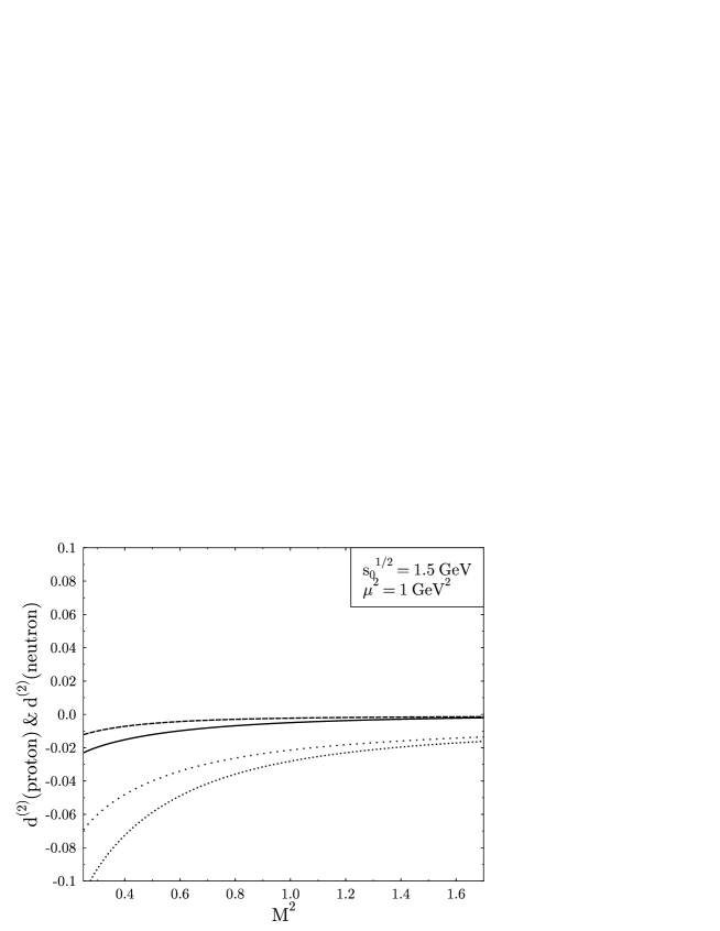
Figure 2: Dependence of $d^{(2)}(proton)$ and $d^{(2)}(neutron)$ on the Borel parameter $M^{2}$. The full line correponds to the $d^{(2)}_{p}$ the dotted line to $d^{(2)}_{n}$. The dashed and space-dotted lines correspond to the results for $d^{(2)}_{\rm BBK}(proton)$ and $d^{(2)}_{\rm BBK}(neutron)$ obtained from the sum rules given in [8].

However, it is more convenient (and usually more accurate) to divide simply the sum rule (S0.Ex8) by the sum rule (S0.Ex10). The coupling constants at the phenomenological side cancel out. The quotient sum rule for the matrix element of twist-3 operator has been plotted in Fig. 1. This figure shows the singlet (S) and nonsinglet (NS) part of $d^{(2)}$. $d^{(2)}(S)=d^{(2)}(u)+d^{(2)}(d)$, $d^{(2)}(NS)=d^{(2)}(u)-d^{(2)}(d)$. The corresponding matrix elements $d^{(2)}(proton)$ and $d^{(2)}(neutron)$ are shown in Fig. 2. For comparison the corresponding sum rules obtained from the the analysis in [8] which employed Ioffe currents only are shown. The corresponding coupling constant $\lambda_{I}^{2}$ is determined from the additional two point sum rule

$$2(2\pi)^{4}\lambda_{I}^{2}e^{-m_{N}^{2}/M^{2}}=M^{6}E_{3}$$

$$+\frac{1}{4}<g^{2}GG>M^{2}E_{1}+\frac{4}{3}(2\pi)^{4}<\bar{q}q>^{2}$$ (20)

which is just the standard sum rule considered by Ioffe. Instead of using a fixed value for $\lambda_{I}^{2}$ we divided the sum rule obtained in [8] by the sum rule (S0.Ex12) which improved the stability considerably. The final values of the matrix elements may then be estimated from the figures by taking $M^{2}\approx m_{N}^{2}$:

$$d^{(2)}(S)=-0.068\pm 0.03\quad d^{(2)}(NS)=0.078\pm 0.03$$

$$d^{(2)}(proton)=-0.006\pm 0.003$$

$$d^{(2)}(neutron)=-0.03\pm 0.01$$ (21)

Errors are due to the $M^{2}$ dependence of the sum rule, see Figure 1 and 2 resp. The uncertainty introduced by the hypothesis of factorization of higher-dimension condensates is discussed below. These values are to be compared with those obtained from the sum rules given in [8]:

$$d^{(2)}_{\rm BBK}(S)=-0.05\pm 0.03\quad d^{(2)}_{\rm BBK}(NS)=0.065\pm 0.03$$

$$d^{(2)}_{\rm BBK}(proton)=-0.003\pm 0.003$$

$$d^{(2)}_{\rm BBK}(neutron)=-0.025\pm 0.01$$

In a recent paper [19] Ross and Roberts have estimated contributions to the sum rule (S0.Ex3) arising from chiral corrections to the phenomenological spectral density. However it is not clear how to take into account the corresponding chiral contributions on the theoretical side of (S0.Ex3), see e.g. [20]. When the necessary “theoretical error” is taken into account, their result agrees with that of [8]. As this error is unavoidably large also in the present case we have not applied the Ross and Roberts analysis to our results.

As in [8] and [18] our sum rule is dominated by the contribution from the highest dimension operators considered i.e., those with coefficients determined to the leading accuracy by tree diagrams. As discussed in [18] this could in principal signal a breakdown of the OPE for the correlator in question which may not allow to make a reliable numerical estimate. In [18] this potentially important problem was settled by an estimate of the contribution from operators of yet higher dimension 10. It was found that the contribution of operators of dimension 10 is likely much smaller than those of dimension 8, which dominated the sum rule in [18]. This is a situation very typical for QCD sum rules. Low-dimension operators are usually numerically unimportant because each extra loop in the definition of the coefficient in front of an operator of lower dimension brings in a small factor $\sim(2\pi^{2})^{-1}$. On the other hand the higher the dimension the stronger is the suppression due to the Borel transfromation. The dominant graphs are therefore usually the lowest dimension tree graphs. In the present case these are the dimension 10 contributions. We expect that as usually still higher dimension contributions starting with dimenision 12 will be small due to the Borel transformation. Unfortunately a quantitative test of these arguments is difficult as very little is known about VEV of operators of dimension 12.

Note also that our calculation involves factorization of the condensate of high dimension. In this respect it is also very similar to the calculation presented in ref. [8]. The factorization of the higher dimensional condensates is a standard technique used in the QCD sum rules. It is necessary to reduce the number of unknown parameters. The physical assumption hidden behind this procedure is the absence of certain higher order correlations in the QCD vacuum. The validity of this assumption has been studied for several simpler condensates [21]. Yet, the knowledge of condensates of dimension 10 is scarce because such condensates rarely appear in calculations. One can even turn this argument around and argue that the good agreement with the previous calculation [8] supports the validity of factorization hypothesis. The BBK result may be treated as a kind of cross check because it relies on a different condensate for the dominant contribution, namely $<\bar{q}q>^{2}m_{0}^{2}$ instead of $<\bar{q}q>^{2}<G^{2}>$ and $<\bar{q}q>^{2}m_{0}^{4}$. The other test is the two point sum rule for the nucleon mass with two $\eta_{G}$ currents [13]. This calculation involves condensates of the dimension 10 and leads to reasonable results.

The agreement between the two calculations is a highly non-trivial check of the QCD sum rules method. The main difference is that in [8] gluons were generated entirely by perturbation theory while in our case they are already present in the interpolating current. As a consequence our correlator (5) has milder singularities than that analysed in [8]. In principle this should be an advantage of our approach but as the current $\eta_{G}(x)$ has two units higher dimension than that of the $\eta_{I}(x)$, the accuracy is diminished by the need to consider higher dimensional condensates. Given an approximate character of the method it is by no means obvious that both approaches give the same results. It seems to us that our results not only give a strong argument in favour of the numerical estimates presented in (S0.Ex13) and (S0.Ex15), but also give a strong support to the credibility of QCD sum rules method. However, neither type of sum rule can be expected to yield very accurate results, because of the slow convergence of the operator product expansion.

We think that taking all the uncertainties into account the following three qualitative statements can be made:

• $|d^{(2)}_{p}|$ and $|d^{(2)}_{n}|$ are smaller than 0.03. The corrections from the twist-3 operator to the Bjorken sum rule and Ellis-Jaffe sum rule are therefore of order $0.013m_{N}^{2}/Q^{2}$ which e.g. for $\int g_{1}^{p}(x)dx$ amounts to a correction of $\sim 5\%$ at $Q^{2}\sim 2{\rm GeV^{2}}$. Note that for a definite answer also $a^{(2)}$ and $f^{(2)}$ have to be taken into account.

• There is a strong isospin asymmetry between $d^{(2)}_{p}$ and $d^{(2)}_{n}$: $|d^{(2)}_{p}|>|d^{(2)}_{n}|$. This isospin asymmetry should manifest itself in a number of spin phenomena [10].

• the sign of $d^{(2)}_{p}$ is negative (in contradiction to the bag model prediction [9]). $d^{(2)}_{n}$ is negative.

Acknowledgements. We would like to thank Vladimir Braun for many usefull discussions and continous encouragement. This work has been supported by KBN grant 2 P302 143 06. A.S. thanks DFG (G.Hess Programm) and MPI für Kernphysik in Heidelberg for support.

References

- [1] J. Ashman et al., Phys. Lett. B206 (1988) 364; Nucl. Phys. 328 (1989) 1
- [2] B. Adeva et al. Phys. Lett. B302 (1993) 533
- [3] E142 Collaboration, M.J.Alguard et al., Phys.Lett. B 261 (1991) 959
- [4] M. Karliner and J. Ellis, “Determination of and the nucleon spin decomposition using recent polarized structure function data”, preprint CERN-TH-7324-94, July 1994, hep–ph@xxx.lanl.gov – 9407287.
-
[5]
E.V. Shuryak and A.I. Vainstein, Nucl.Phys. B199 (1982) 451;
Nucl.Phys. B201 (1982) 141;
B. Ehrnsperger, L. Mankiewicz, and A. Schäfer, Phys.Lett. B323 (1994) 439. - [6] S.A. Larin, F.V. Tkachev, and J.A.M. Vermaseren, Phys. Rev. Lett. 66 (1991) 862; S.A. Larin and J.A.M. Vermaseren, Phys. Lett. B 259 (1991) 345.
- [7] R.L. Jaffe, Comments Nucl.Part.Phys. 19 (1990) 239.
- [8] I.I. Balitsky, V.M. Braun, and A.V. Kolesnichenko, Phys.Lett. B242 (1990) 245; Phys.Lett. B318 (1993) 648 (E).
- [9] X. Ji and P. Unrau, Phys.Lett. B333 (1994) 228.
- [10] B. Ehrnsperger, L. Mankiewicz, A. Schäfer, and W. Greiner, Phys.Lett. B321 (1993) 121.
- [11] R. Horsley (HLRZ Jülich), private communication
- [12] B.L. Ioffe, Nucl.Phys.B188 (1981) 317; (E) ibid. B191 (1981) 71.
- [13] V.M. Braun, P. Górnicki, L. Mankiewicz, and A. Schäfer, Phys.Lett. 302 (1993) 291.
- [14] I.I. Balitsky, Phys.Lett.114B (1982) 53.
-
[15]
I.I. Balitsky and V. Yung, Phys.Lett. 129B, (1983) 328;
I.I. Balitsky, A.V. Kolesnichenko and A.V. Yung, Phys.Lett. 157B, (1985) 309. - [16] M. Jamin and M.E. Lautenbacher, Comput. Phys. Commun. 74 (1993) 265.
- [17] G. t’Hooft, M.Veltman, Nucl. Phys., B44 189 (1972); C.G.Bollini, J.J.Giambiagi, Nuovo Cim., B12, 20 (1972); J.F.Ashmore, Lett. Nuovo Cim., 4, 289 (1972); G.M.Cicuta, R.Montaldi, Lett. Nuovo Cim., 4, 329 (1972)
- [18] V.M. Braun and A.V. Kolesnichenko, Nucl.Phys. 283B (1987) 723.
- [19] G.G. Ross and R.G. Roberts, Phys.Lett. B322, (1994) 425.
- [20] D. K. Griegel and T. D. Cohen, “QCD sum rules vs. chiral perturbation theory”, preprint UMPP # 94-136, hep–ph@xxx.lanl.gov – 9405287
- [21] A.R. Zhitnitskii, Yad. Fiz. 41 (1985) 805; ibidem, 1305; ibidem, 1331.