Abstract

We compare the results of the fixed-flavor scheme calculation of Laenen, Riemersma, Smith and van Neerven with the variable-flavor scheme calculation of Aivazis, Collins, Olness and Tung for the case of neutral-current (photon-mediated) heavy-flavor (charm and bottom) production. Specifically, we examine the features of both calculations throughout phase space and compare the structure function $F_{2}(x,Q^{2})$. We also analyze the dependence of $F_{2}$ on the mass factorization scale $\mu$. We find that the former is most applicable near threshold, while the latter works well for asymptotic $Q^{2}$. The validity of each calculation in the intermediate region is dependent upon the $x$ and $Q^{2}$ values chosen.

1 Introduction

Several experimental groups [1] have studied the semi-inclusive deeply inelastic scattering (DIS) process for heavy-quark production (Figure 1)

$${}\ell_{1}(\ell_{1})+N(P)\rightarrow\ell_{2}(\ell_{2})+Q(p_{1})+X(P_{X}).$$ (1)

Most analyses of this process assume that the hadron is comprised only of the massless gluon ($g$), up ($u$), down ($d$) and strange ($s$) quarks, while the charm ($c$), bottom ($b$), and top ($t$) quarks are treated as massive objects which are strictly external to the hadron.

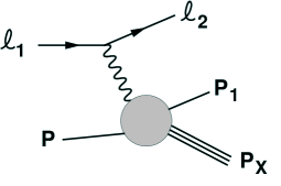
Figure 1: The basic semi-inclusive deeply inelastic scattering process, $\ell_{1}(\ell_{1})+N(P)\longrightarrow\ell_{2}(\ell_{2})+Q(p_{1})+X(P_{X})$.

This view of the heavy quarks as external to the hadron is appropriate when the energy scale of the process $\mu_{\rm phy}$ (for example the center-of-mass energy $\sqrt{s}$) is not large compared to the mass of the heavy quark, i.e. $M_{Q}\lower 2.15277pt\hbox{$\stackrel{{\scriptstyle<}}{{\sim}}$}\mu_{\rm phy}$. For most fixed-target facilities, this condition holds for the $c$, $b$ and $t$ quarks [3]. We are therefore justified in excluding $c$, $b$, and $t$ as constituents of the hadron in the QCD-improved quark-parton model (QPM) for this case.

With new data from HERA, the electron-proton collider at DESY, we can investigate the DIS process in a very different kinematic range from that available at fixed-target experiments [3]. In this new realm, the important question is: Should the $c$ and $b$ quarks be considered as partons, or as heavy objects extrinsic to the hadron? Given that HERA extends the kinematic reach of the DIS process by two orders of magnitude, we can not expect our assumptions that were valid for fixed-target processes to hold in a completely different kinematic regime.

Aivazis, Collins, Olness and Tung (ACOT) have discussed this issue at length in reference [4] and approach the problem by invoking the variable flavor scheme (VFS), which varies the number of partons according to the relevant energy scale $\mu_{\rm phy}$. The fundamental physical insight to the VFS is that in the region $M_{Q}\,\gg\,\mu_{\rm phy}$, the heavy quark should be excluded as a constituent of the hadron as it is kinematically inaccessible. However, when $M_{Q}\,\ll\,\mu_{\rm phy}$ the heavy quark should be included as a parton since $M_{Q}$ is insignificant compared to $\mu_{\rm phy}$. Although the physics is unambiguous in these kinematic extremes, most experimental data lies in between these clear-cut regions. In the intermediate region, the renormalization scheme of Collins, Wilczek and Zee (CWZ) [5] provides a well-defined transition between these two extreme kinematic domains.

The issue of what constitutes a parton also points to an inconsistency between traditional charged-current and neutral-current heavy-quark production calculations [4]. When considering charged-current processes, one begins with the purely electroweak process $W+q\to Q$, as shown in Figure 2a. For neutral-current processes, the traditional approach is to begin with the ${\cal O}(\alpha_{s}^{1})$ process $\gamma^{*}+g\to Q+\overline{Q}$, as shown in Figure 2b. As we work in the new kinematic regime spanned by HERA, the concept of a ‘heavy’ quark becomes a relative term depending upon the magnitudes of the kinematic variables involved. Traditional distinctions between the charged-current and neutral-current calculations should vanish as the characteristic energy scale becomes significantly larger than the heavy-quark mass. ACOT implements the CWZ renormalization scheme and treats both charged-current and neutral-current heavy-flavor production in the consistent fashion of beginning both calculations at ${\cal O}(\alpha_{s}^{0})$.

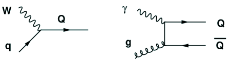
Figure 2: 2a) The ${\cal O}(\alpha_{s}^{0})$ flavor excitation (FE) process, shown here for the charged-current case. 2b) The ${\cal O}(\alpha_{s}^{1})$ flavor creation (FC) process, shown here for the neutral-current case.

Laenen, Riemersma, Smith and van Neerven (LRSN) have calculated heavy-quark production for DIS photon exchange, beginning with the ${\cal O}(\alpha_{s}^{1})$ photon-gluon fusion process and including the complete ${\cal O}(\alpha_{s}^{2})$ radiative corrections in reference [6]. Figure 3 displays some of the relevant ${\cal O}(g^{2})$ tree-level and ${\cal O}(g^{3})$ virtual Feynman diagrams involved, where $g$ is the QCD coupling strength and is given by $\alpha_{s}=g^{2}/4\pi$. LRSN calculates from the viewpoint that the produced heavy quark is generated from an initial-state gluon or lighter quark. For example, in producing $c$ quarks, LRSN assumes the parton initiating the heavy-quark production process to be the $g$, $u$, $d$ or $s$ quark. The same tenet holds for $b$ production, only the $c$ quark would be included as a massless initial-state parton as well.

Figure 3: Pictorial representation of the fixed flavor scheme (FFS) calculation of LRSN. 3a) The ${\cal O}(\alpha_{s}^{1})$ flavor creation (FC) contribution. 3b), 3c), 3d), and 3e) An illustrative subset of the complete set of ${\cal O}(\alpha_{s}^{2})$ diagrams contributing to the complete LRSN calculation.

Another feature of the LRSN calculation is that it provides additional information on inclusive differential cross section distributions. At ${\cal O}(\alpha_{s}^{1})$, the heavy quark and antiquark are produced back to back in the $\gamma^{*}$-parton center of momentum frame, and at ${\cal O}(\alpha_{s}^{2})$, the additional influences of the gluon radiation and the $\gamma^{*}q$ channel have also been calculated in [7]. LRSN gives additional insight into the differential distributions, which is particularly useful from the experimental point of view.

The subject of this paper is a vigorous comparison of the advantages of each calculation, as well as a glimpse of future prospects including a merging of the two calculations to produce a three-order result which should have excellent predictive power for heavy-flavor structure functions at HERA.

2 Kinematics

While Figure 1 shows the general deeply inelastic scattering (DIS) process, we shall focus specifically on neutral-current heavy-flavor production via a photon exchange as described by the sub-process $\gamma^{*}(q)+N(P)\longrightarrow Q(p_{Q})+X(P_{X})$. We define $Q^{2}=-q^{2}$, where $q$ is the four momentum of the virtual photon exchanged, $y=(P\cdot q)/(P\cdot\ell_{1})$ is the fractional energy transfer, and $x=Q^{2}/(2P\cdot q)$ is the Bjorken $x$ variable. The cross section is obtained from the structure functions via

$${}\frac{d^{2}\sigma}{dx\,dy} = \frac{2ME_{1}}{\pi}\frac{G_{1}G_{2}}{n_{\ell}}\left\{g^{2}_{+l}\left[xF_{1}\,y^{2}+F_{2}\,\left[(1-y)-\left(\frac{Mxy}{2E_{1}}\right)\right]\right]\pm g^{2}_{-l}\left[xF_{3}\,y\left(1-\frac{y}{2}\right)\right]\right\}\quad.$$ (2)

$E_{1}$ is the energy of the incoming lepton, $M$ is the mass of the hadron being probed, $G_{i}=g^{2}_{B_{i}}/(Q^{2}+M^{2}_{B_{i}})$ is a shorthand for the boson coupling and the propagator, $n_{\ell}$ is the number of polarization states of the incoming lepton, and $g^{2}_{\pm l}=g^{2}_{Ll}\pm g^{2}_{Rl}$, where $g_{Ll}$ and $g_{Rl}$ refer to the chiral couplings of the vector boson to the leptons.

3 ACOT Calculation

The ACOT calculation makes use of the ${\cal O}(\alpha_{s}^{0})$ and ${\cal O}(\alpha_{s}^{1})$ processes to obtain a two-order result, cf. Figure 2 and Figure 4. The ${\cal O}(\alpha_{s}^{0})$ result uses the standard QCD evolution to resum the iterative gluon and quark splittings to give the parton distribution function (PDF) of the heavy quark.

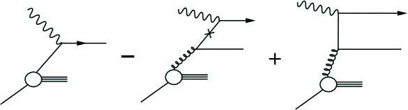
Figure 4: Pictorial representation of the variable flavor scheme (VFS) calculation of ACOT. 4a) The ${\cal O}(\alpha_{s}^{0})$ flavor excitation (FE) contribution. 4b) The schematic representation of the subtraction term. The $\times$ on the intermediate quark line indicates a convolution between the ${\cal O}(\alpha_{s}^{1})$ $g\to q$ splitting (lower portion of the diagram) with the ${\cal O}(\alpha_{s}^{0})$ process (upper portion of the diagram). 4c) The ${\cal O}(\alpha_{s}^{1})$ flavor creation (FC) contribution.

The ${\cal O}(\alpha_{s}^{0})$ term is straightforward, and is represented by

$${}{{}^{0}F}=F(\hbox{${\cal O}(\alpha_{s}^{0})$}) = f_{N}^{Q_{i}}\otimes\widehat{F}^{(0)}(\gamma^{*}Q_{i}\rightarrow Q_{i})\quad,$$ (3)

where $f_{N}^{Q_{i}}$ denotes the parton distribution function for a nucleon $N$ producing a quark $Q_{i}$, and the $\widehat{F}^{(0)}(\gamma^{*}Q_{i}\rightarrow Q_{i})$ is the lowest-order partonic structure function for the initial-state heavy quark $Q_{i}$ to absorb a virtual photon $\gamma^{*}$ and enter the final state. We introduce the shorthand $F({\cal O}(\alpha_{s}^{n}))={{}^{n}F}$. The $\otimes$ represents the convolution which is the integral over the momentum fraction carried by the initial state parton $i$

$${}f^{i}_{N}\otimes\widehat{F} = \int_{x}^{1}\ \frac{d\xi}{\xi}\ f^{i}_{N}\left(\frac{x}{\xi},\mu_{f}\right)\ \widehat{F}\left(\xi,\frac{Q}{\mu_{f}},\alpha_{s}(\mu_{r})\right)\quad.$$ (4)

where $\xi=k^{+}/P^{+}$ is the ratio of the “$+$”-component of the parton momentum $k^{+}$ to the hadron momentum $P^{+}$ in light cone coordinates, $\mu_{r}$ is the renormalization scale, and $\mu_{f}$ is the mass factorization scale. For the remainder of this paper, we shall not distinguish between $\mu_{r}$ and $\mu_{f}$, and we choose $\mu_{r}=\mu_{f}\equiv\mu$. Although the partonic structure function $\widehat{F}$ and the evolution of the PDF with mass factorization scale $\mu$ are calculable in perturbative QCD, the $\xi$-dependence of the PDF is not and must be derived from experimental data.

Handling the collinear and infrared divergences of the $F(\hbox{${\cal O}(\alpha_{s}^{1})$})$ requires careful application of the factorization formula as illustrated in the ACOT paper. The complete ${}^{1}F$ contribution in VFS is given by

$${}{{}^{1}F}_{\scriptscriptstyle V}=F_{\scriptscriptstyle V}(\hbox{${\cal O}(\alpha_{s}^{1})$})={{}^{1u}F}_{\scriptscriptstyle V}-{{}^{1s}F}_{\scriptscriptstyle V} = f_{N}^{g}\otimes\widehat{F}^{(1)}(\gamma^{*}g\rightarrow Q_{i}\overline{Q}_{i})-f_{N}^{g}\otimes f_{g}^{Q_{i}\,(1)}\otimes\widehat{F}^{(0)}(\gamma^{*}Q_{i}\rightarrow Q_{i})$$

${{}^{1u}F}_{\scriptscriptstyle V}$ is the ‘unsubtracted’ ${\cal O}(\alpha_{s}^{1})$ contribution, meaning the collinear singularities are still present, and ${{}^{1s}F}_{\scriptscriptstyle V}$ is the ‘subtraction’ term which cancels the singularities and renders ${}^{1}F$ finite. The $V$ subscript indicates the use of the VFS. The reason for separating ${}^{1}F$ into these two pieces will become clear in Section 5, where the K-factors are discussed. Here, $f_{g}^{Q_{i}\,(1)}$ is the perturbative ${\cal O}(\alpha_{s}^{1})$ splitting function for the process $g\rightarrow Q_{i}$ and is given by

$${}f_{g}^{Q_{i}\,(1)} = {\alpha_{s}(\mu)\over 4\pi}\ C_{R}\ \ln\left({\mu^{2}\over M_{Q}^{2}}\right)\ P_{g\rightarrow q}(x)\ \theta(\mu^{2}-M_{Q}^{2}),$$ (6)

where $P_{g\rightarrow q}(x)=t_{F}\,(1-2x+2x^{2})$. In SU(N), $C_{R}=(N^{2}-1)/2N$ and $t_{F}=1/2$. Note that $f_{g}^{Q_{i}\,(1)}=0$ when $\mu\leq M_{Q}$, and evolves continuously from zero for $\mu\geq M_{Q}$.

4 LRSN Calculation

The LRSN calculation uses a fixed flavor scheme (FFS), which sets the number of active flavors to a constant, regardless of the energy scale $\mu_{\rm phy}$ of the production process. For example, when considering $b$ production the number of light flavors would be four.

The lowest-order FFS ${\cal O}(\alpha_{s}^{1})$ term is given by

$${}{{}^{1}F}_{\scriptscriptstyle F}=F_{\scriptscriptstyle F}(\hbox{${\cal O}(\alpha_{s}^{1})$}) = f_{N}^{g}\otimes\widehat{F}^{(1)}(\gamma^{*}g\rightarrow Q_{i}\overline{Q}_{i}).$$ (7)

Mass factorization is not necessary at ${\cal O}(\alpha_{s}^{1})$ in FFS since the mass of the heavy quark is explicitly assumed to be non-zero throughout the calculation, and the initial-state heavy quark contribution is not included. Note the ${{}^{1}F}_{\scriptscriptstyle F}$ contribution in this scheme corresponds to the ‘unsubtracted’ ${{}^{1u}F}_{\scriptscriptstyle V}$ contribution of VFS. We make use of this fact when we compare the K-factors in Section 8.

LRSN has computed the Feynman diagrams shown in Figure 3 to give the complete ${\cal O}(\alpha_{s}^{2})$ result. After cancelling the infrared divergences and performing the necessary renormalization, the mass factorization is done according to

$${}{{}^{2}F}=F(\hbox{${\cal O}(\alpha_{s}^{2})$})={{}^{2u}F}-{{}^{2s}F} = f_{N}^{g}\otimes\widehat{F}^{(2)}(\gamma^{*}g\rightarrow Q_{i}\overline{Q}_{i}g)+\sum_{a}f_{N}^{q_{a}}\otimes\widehat{F}^{(2)}(\gamma^{*}q_{a}\rightarrow Q_{i}\overline{Q}_{i}q_{a})-\,{{}^{2s}F}\,,$$

where all the contributions from initial-state partons light relative to the produced heavy quark are summed. As before, we recognize the first term as the ‘unsubtracted’ ${}^{2u}F$(${\cal O}(\alpha_{s}^{2})$) contribution, and the second term as the ‘subtraction’ term ${}^{2s}F$(${\cal O}(\alpha_{s}^{2})$) which removes the collinear mass singularity from the radiation of a gluon by the incoming massless quark or gluon. Note the ‘subtraction’ term does not subtract the $M_{Q}\rightarrow 0$ singularity. Mass factorization is not necessary as $M_{Q}^{2}/Q^{2}$ is explicitly assumed to be non-zero and the initial-state heavy quark contribution is assumed absent. For additional details, see references [6] and [7]. At ${\cal O}(\alpha_{s}^{2})$ the FFS subscript is superfluous since no confusion is present at this order.

5 K-factors

The two calculations each include a different subset of the complete set of higher-order corrections. The comparison of the two approaches will determine to what extent these calculations pick up similar higher-order contributions, and can be used to estimate the magnitude of the corrections not included by either approach. To facilitate this comparison, we shall focus on the $F_{2}$ K-factors of each calculation as a function of $x$ and $Q^{2}$. For the LRSN calculation, we define the K-factor to be

$${}K_{LRSN} = \frac{{{}^{1}F}_{\scriptscriptstyle F}+{{}^{2}F}}{{{}^{1}F}_{\scriptscriptstyle F}}\equiv\frac{{{}^{1u}F}_{\scriptscriptstyle V}+{{}^{2}F}}{{{}^{1u}F}_{\scriptscriptstyle V}}\,,$$ (9)

where the $K_{LRSN}$ indicates the K-factor is coming from the LRSN ${\cal O}(\alpha_{s}^{2})$ contributions.

For ACOT, we define the K-factor as

$${}K_{ACOT} = \frac{{{}^{0}F}_{\scriptscriptstyle V}+{{}^{1}F}_{\scriptscriptstyle V}}{{{}^{1u}F}_{\scriptscriptstyle V}}\equiv\frac{{{}^{1u}F}_{\scriptscriptstyle V}+({{}^{0}F}_{\scriptscriptstyle V}-{{}^{1s}F}_{\scriptscriptstyle V})}{{{}^{1u}F}_{\scriptscriptstyle V}}\,,$$ (10)

where $K_{ACOT}$ indicates the K-factor is coming from the ACOT ${\cal O}(\alpha_{s}^{0})$ contribution. $K_{ACOT}$ is defined in this manner because it is the ${{}^{1}F}_{\scriptscriptstyle F}\equiv{{}^{1u}F}_{\scriptscriptstyle V}$ contribution which is common to both calculations. Therefore, we use this common term to set the scale of comparison in the denominator of the K-factor. Secondly, in the threshold region ($Q\simeq M_{Q}$), the production cross section is dominated by the ${\cal O}(\alpha_{s}^{1})$ process. Viewing the ${\cal O}(\alpha_{s}^{0})$ process as a perturbation on the dominant ${\cal O}(\alpha_{s}^{1})$ process, we see Equation (10) is the natural definition of the K-factor.

Both of these points become clear when the second form of Equation (10) is compared with Equation (9). The higher-order contributions for the LRSN calculation are contained in the ${}^{2}F$ term, whereas ${{}^{0}F}-{{}^{1s}F}$ yields the contribution for the ACOT calculation.

6 Parton Distributions for Heavy Quarks: The VFS Approach

The VFS calculation of ACOT uses the CWZ renormalization scheme to incorporate the heavy quark into the QPM. The fundamental idea here is that at low energy scales ($Q\ll M_{Q}$), we do not want to treat the heavy quark as a constituent of the hadron. However, at high energy scales ($Q\gg M_{Q}$), the mass of the ‘heavy’ quark is negligible and we should therefore treat this quark on the same footing as the other massless partons. The concept that there should be a democracy among the quarks in the limit $Q/M_{Q}\rightarrow\infty$ forces us to introduce the heavy quark as a parton at some intermediate energy scale which is typically related to the quark mass. The choice of this scale is intimately connected to the choice of renormalization scheme [8], [9].

The motivation to include the heavy quark as a constituent of the hadron is more than aesthetic. When computing physical cross sections in the context of perturbation theory, we find that our perturbation expansion is not simply an expansion in powers of $\alpha_{s}$. As we compute higher-order subprocesses, we gain logarithms involving the various energy scales in the problem (such as $\ln(Q/M_{Q})$). Therefore, we find that our perturbation series is actually an expansion in $\alpha_{s}\ln(Q/M_{Q})$. In the limit $Q/M_{Q}\rightarrow\infty$, we will clearly have a divergent series unless we can resum these logarithmic terms.

The QCD evolution of the parton distribution functions does precisely this resummation for the partons. It sums an infinite set of quark and gluon splittings, thereby taking all such logarithmic contributions into account. To be perfectly clear, these resummations are done in both LRSN and ACOT for the light quarks and the gluon. The only difference is in the way the heavy quark is treated. For ACOT, it is incorporated into the PDF, and for LRSN, it only enters in the final state as a product of an interaction of a light quark or gluon with the virtual photon.

The goal of the ACOT calculation is to use this same technique to resum the multiple splittings arising from the QCD evolution of the heavy-quark distribution. The result is to reorganize the perturbation expansion such that the singular $\alpha_{s}\ln(Q/M_{Q})$ terms are split into an $\alpha_{s}\ln(Q/\mu)$ term which remains in the hard scattering Wilson coefficient and an $\alpha_{s}\ln(\mu/M_{Q})$ term which is absorbed into the heavy-quark PDF. The end result is that the perturbation series then becomes an expansion in powers of $\alpha_{s}\ln(Q/\mu)$, and we retain the freedom to adjust $\mu$ to optimize the convergence of the series.

This is clearly the correct approach in the asymptotic limit $Q/M_{Q}\rightarrow\infty$ but how well does it work in the kinematic regime of present accelerators? The only way to answer this question is to compare ACOT with a separate calculation such as LRSN.

7 Kinematic Regimes

7.1 Collinear/On-Shell vs. Large $P_{T}$/Virtual

The VFS approach (ACOT) resums an infinite subset of diagrams (Figure 4) within the PDF of the heavy quark, cf., via the flavor excitation (FE) (Figure 3a). Because the heavy quark is treated as a parton for this set of contributions, the phase space of the heavy quark is restricted to the on-shell collinear region. In the asymptotic limit $\mu\to\infty$, the on-shell collinear region is the dominant region of phase space but how large is this contribution in the threshold region $\mu\simeq M_{Q}$?

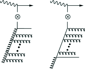
Figure 5: An illustrative subset of the class of diagrams which are summed by the QCD evolution of the heavy quark PDF in the variable flavor scheme (VFS) calculation of ACOT. The $\otimes$ indicates a convolution between the heavy quark PDF (lower portion of the diagram) and the ${\cal O}(\alpha_{s}^{0})$ process (upper portion of the diagram).

The FFS calculation (LRSN) does not treat the heavy quark as a parton. Instead, the heavy-quark contribution is included explicitly into the hard scattering via the flavor-creation (FC) process (Figure 3b). In this case, the heavy-quark contributions are not restricted in phase space. The splitting of the initial state gluon is only included up to ${\cal O}(\alpha_{s}^{2})$ but covers the collinear on-shell region as well as the region where the $t$-channel heavy quark is far off-shell. We therefore expect LRSN to provide the best results when the $t$-channel heavy quark is highly virtual, but how much of the on-shell collinear region does LRSN include?

We want to investigate how important the roles that the flavor creation (LRSN calculation) and the flavor excitation (ACOT calculation) processes play when in the threshold region ($Q\sim M_{Q}$), in the intermediate transition region ($Q\,>\,M_{Q}$), and in the asymptotic region ($Q\gg M_{Q}$).

7.2 Threshold Region

In the threshold region, we do not expect the QCD evolution of the heavy quark PDF to make a significant contribution since the heavy-quark evolution begins at scale $\mu\sim M_{Q}$, and ends at scale $\mu\sim Q$ not significantly larger than $M_{Q}$. More specifically, in the threshold region, the heavy quark will typically be produced far off-shell such that the dominant region of phase space is the virtual region. Since the ACOT calculation picks up primarily the on-shell region of phase space while the LRSN calculation picks up the entire phase space, we expect the LRSN calculation should make the better prediction in this region.

In fact, if the physical threshold for heavy-quark production is below the threshold for introducing the heavy quark into the PDF ($\mu<M_{Q}$), then there will be no contribution from the heavy-quark QCD evolution since $f_{Q}(\mu<M_{Q})=0$. In the limit, both the ${}^{0}F$ and ${}^{1s}F$ contributions will vanish so that only ${}^{1u}F$ remains. It is now evident why we defined the K-factor for the ACOT calculation by Equation (10). In this limit, the K-factor is unity, and there is no contribution from higher orders in this kinematic regime. On the other hand, since the LRSN calculation computes the higher order corrections for a virtual heavy-quark exchange, the result is a non-trivial K-factor near threshold.

We conclude that near threshold, the dominant region of phase space is the virtual region. We therefore expect the LRSN calculation to determine more accurately the higher-order contributions in this region.

7.3 Asymptotic Region

We now consider the asymptotic region where $\mu_{\rm phy}\gg M_{Q}$. In this region, we can essentially neglect the mass of the heavy quark in comparison to the characteristic energy scale of the process, $\mu_{\rm phy}$. Because the mass of the ‘heavy’ quark is small relative to $\mu_{\rm phy}$, the ‘heavy’ quark is easily produced on-shell with relatively little transverse momentum (of order $M_{Q}$) as compared to its longitudinal momentum (of order $\mu_{\rm phy}$) in the $\gamma^{*}$-hadron center of momentum frame.

Equivalently, the QCD evolution will now be significant because there is a large region (from $M_{Q}$ to $\mu$) over which the evolution can build up the heavy-quark parton distribution. Therefore, we expect the dominant region of phase space is the collinear region, and that the ACOT approach should correctly resum the important higher order contributions.

In this asymptotic limit, the collinear portion of ${}^{2}F$ in LRSN (see Figure 3) will be contained within the ACOT result as are the other higher-order gluon ladder graphs. If the phase space is dominated by the collinear region then the ACOT calculation is well suited to make accurate predictions in the asymptotic region since the dominant terms, the infinite set of recursive quark and gluon splittings, have been resummed. The singular $\alpha_{s}\ln(Q/M_{Q})$ present in the LRSN calculation have been reorganized in ACOT (absorbed into the heavy-quark PDF) to leave only terms of order $\alpha_{s}\ln(Q/\mu)$.

If it were to happen that the terms of order ${\cal O}(\alpha_{s}^{3})$ and higher were a negligible contribution to the ${\cal O}(\alpha_{s}^{1})$ and ${\cal O}(\alpha_{s}^{2})$ terms computed in the LRSN calculation, then we would expect the ACOT and LRSN calculations to match in this asymptotic region. Conversely, the difference between these calculations in this region is indicative of the size of the terms of order ${\cal O}(\alpha_{s}^{3})$ and higher which have been resummed in the QCD evolution of the heavy quark parton distributions.

While the ACOT calculation is expected to provide the more accurate results at asymptotic $Q^{2}$, the question arises: what $Q^{2}$ qualifies as asymptotic? As $Q^{2}$ gets large then $\alpha_{s}\ln(Q^{2}/M_{Q}^{2})$ can grow to ${\cal O}(1)$ and spoil the convergence of the perturbation series. Investigating this problem in a cursory way, we present the expression for $\alpha_{s}$ at the two-loop level to be

$${}\alpha_{s}(\mu) = \frac{4\pi}{\beta_{1}\ln\left(\mu^{2}/\Lambda_{QCD}^{2}\right)}\ \left[1-\frac{\beta_{2}\ln\ln\left(\mu^{2}/\Lambda_{QCD}^{2}\right)}{\beta_{1}^{2}\ln\left(\mu^{2}/\Lambda_{QCD}^{2}\right)}\right]\,,$$ (11)

where $\beta_{1}$ and $\beta_{2}$ are given by

$${}\beta_{1} = \frac{11}{3}C_{A}-\frac{4}{3}n_{f}\,t_{F}\,,$$ (12)

$$\beta_{2} = \frac{34}{3}C_{A}^{2}-\frac{20}{3}C_{A}n_{f}\,t_{F}-4C_{F}n_{f}\,t_{F}\,,$$ (13)

$n_{f}$ is the number of light flavors, $C_{A}=N$, $C_{F}=(N^{2}-1)/2N$, $t_{F}=1/2$ for QCD, and $N$ is from the $SU(N)$ nature of QCD. We see from this expression for $\alpha_{s}$ that while $\ln(Q/M_{Q})$ is growing with increasing $Q$, this effect will be offset by the diminishing of $\alpha_{s}$ with the dominant $\ln(\mu/\Lambda)$ term in the denominator since $\mu$ must be chosen as a function of $Q$ and/or $M_{Q}$. Thus it is not clear what $Q$ we can consider to be asymptotic, and we need to analyze the results of this comparison to draw definite conclusions.

7.4 Intermediate Region

The intermediate region is the most interesting as the heavy-quark production process is a complex interplay of all available mechanisms. Complications arise because we have no limiting behavior to guide us as we analyze the results of each calculation. What we do know is that the LRSN calculation should provide the most accurate results in the threshold region and ACOT should in the asymptotic. What remains to be seen is how and where the transition occurs from one to the other. We have little intuition about this region, and must rely on the comparison of these two calculations to give us insight into the physics.

One portent of future progress in heavy-flavor production, the merging of the two calculations would be most effective in this region, as neither the flavor excitation process nor the flavor creation process should be the dominant mechanism. The three-order calculation that combines the ACOT and LRSN calculations into one should have the virtues of both approaches, have considerably reduced mass factorization scale dependence, and allow us to make very accurate predictions to compare with the data from HERA. This effort is currently underway [10].

8 Comparison

We present our results using the CTEQ2 PDF set [11], which begins the charm quark QCD evolution $\mu_{0}=m_{c}=1.6$ GeV, and the bottom quark QCD evolution at $\mu_{0}=m_{b}=5.0$ GeV, For $\mu\leq\mu_{0}$, the heavy-quark density in the hadron vanishes, $f_{Q}(x,\mu\,<\,M_{Q})=0$. For the scale $\mu$, we make the choice

$${}\mu^{2}=\cases{M_{Q}^{2}&if $Q^{2}<M_{Q}^{2}$\cr M_{Q}^{2}+cQ^{2}(1-\frac{M_{Q}^{2}}{Q^{2}})^{n}&if $Q^{2}\geq M_{Q}^{2}$\cr}$$ (14)

with $c=1/2$ and $n=2$ as discussed in ACOT.

8.1 C-Quark Production

8.1.1 Charm $F_{2}$ vs. $\{x,Q^{2}\}$

We now present a series of plots showing the $F_{2}$’s for various values of $Q^{2}$ vs. $x$. The $F_{2}$ K-factors are shown to facilitate comparison between the different curves. The values of the $F_{2}$ structure functions are also shown on a log-log plot to indicate difference in an absolute sense, and to gauge the contribution to the cross section which is proportional to the integral of $F_{2}$ over $x$.

We refer to the curves as FE for the ${\cal O}(\alpha_{s}^{0})$ flavor excitation process, FC for the ${\cal O}(\alpha_{s}^{1})$ flavor creation process, ACOT for the complete VFS calculation and LRSN for the complete FFS calculation. The FC curve is not shown as this is the denominator in the definition of the K-factors. (Trivially, $K_{FC}=1$.)

For $Q=1.778$ GeV, (Figure 6) the FE K-factor essentially vanishes as compared to the other contributions because $f_{c}(x,\mu)\simeq 0$. This result matches our expectation that “heavy-quark” partons should not contribute at low energy scales. The ACOT K-factor is approximately equal to one; that is, the ACOT reduces to the FC result in the low energy limit. This is because we have $f_{c}(x,\mu)\simeq f^{g}_{N}(x,\mu)\otimes f_{g}^{c\,(1)}(x,\mu)$ in the threshold region causing $({{}^{0}F}_{\scriptscriptstyle V}-{{}^{1s}F}_{\scriptscriptstyle V})\simeq 0$, and therefore $K_{ACOT}\simeq 1$. The rise in the FE and ACOT K-factors is due to the difference between the one-particle and two-particle phase space factors in the threshold region ($x\to x_{max}$). The one-particle final state requires the partonic center-of-mass energy $\sqrt{s}>M_{Q}$ and the two-particle final state demands $\sqrt{s}>2M_{Q}$. This causes the K-factors for ACOT to diverge for $2M_{Q}>\sqrt{s}>M_{Q}$, where $s=Q^{2}(1-x)/x$. The rise in the LRSN K-factor is attributed to the dominance of the ${\cal O}(\alpha_{s}^{2})$ contributions over the ${\cal O}(\alpha_{s}^{1})$ result, as can be seen at the partonic level in Figures 6a and 7a of [6]. The effect on the absolute value of $F_{2}$ and the cross sections is negligible as can be seen in Figure 6b. Clearly, in this low $Q$-region, the LRSN calculation is the most appropriate because the FC photon-gluon fusion process is the dominant one, the ${\cal O}(\alpha_{s}^{2})$ corrections to that channel are included in the LRSN calculation and provide a non-trivial K-factor. The corrections at large $x$ are primarily a result of the Coulomb exchange of a gluon between the final-state heavy quark and antiquark as well as initial-state-gluon bremsstrahlung.

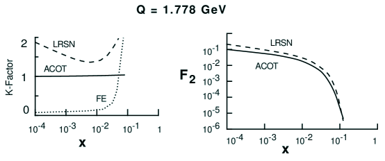
Figure 6: 6a) the K-factor, and 6b) the structure function $F_{2}(x,Q^{2})$ for $c$-production at $Q=1.778GeV$.

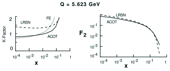
Figure 7: 7a) the K-factor, and 7b) the structure function $F_{2}(x,Q^{2})$ for $c$-production at $Q=5.623GeV$.

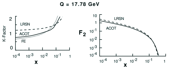
Figure 8: 8a) the K-factor, and 8b) the structure function $F_{2}(x,Q^{2})$ for $c$-production at $Q=17.78GeV$.

At $Q=5.623$ GeV (Figure 7), the FE $F_{2}$ result has increased significantly and approaches the other curves. This very fast evolution of the FE result makes it unreliable for predicting heavy-quark production. The ACOT K-factor now deviates from unity as the imperfect cancellation between ${{}^{0}F}_{\scriptscriptstyle V}$ and ${{}^{1s}F}_{\scriptscriptstyle V}$ signals the existence of non-trivial contributions from the heavy-quark PDF evolution. The fast evolution of the heavy quark in the threshold region (due to abundant gluons) generates important contributions for relatively low values of $Q$. However the subtraction prescription ensures the result is reliable (in contrast to the FE process), as we shall confirm when we examine the $\mu$-dependence. The LRSN K-factor decreases at small $x$, and flattens slightly. This decrease at small $x$ is due in large part to the cancellation between the mass factorization logarithmic terms and the mass factorization scale independent terms at large parton-photon center-of-mass energies $s$. For additional discussions, see pp.192-196 of reference [6].

At $Q=17.78$ GeV (Figure 8), the FE, ACOT, and LRSN results have similar shapes. The K-factors are all monotonically increasing vs. $x$, with a large rise in the threshold ($x\to x_{max}$) region. In the range above $Q=17.78\,GeV$, the general characteristics are similar to this Figure 8.

8.1.2 Charm $F_{2}$ vs. $\mu$

We now present a series of plots of the $\mu$-dependence of $F_{2}$ for particular $x$ and $Q^{2}$ values accessible to HERA.

For $x=0.001$ and $Q=3.162$ GeV (Figure 9), the FE result has a large $\mu$-dependence. The FE process is driven by the heavy-quark PDF and vanishes at small $\mu$ because $f_{c}(x,\mu)=0$ for $\mu\leq m_{c}$. As $\mu$ increases above $m_{c}$, $f_{c}(x,\mu)$ increases quickly due to the abundance of gluons and the dearth of heavy quarks near threshold. Clearly, the FE result is extremely sensitive to the particular choice of scale, as well as the choice of factorization scheme which determines where to start the heavy-quark evolution. As anticipated, the apparent agreement between the FE result and the other results as seen in the previous subsection is merely an accident due to a prudent choice of scale, and cannot provide stable results. The LRSN result is quite flat, and the ACOT calculation exhibits a rather marked dependence on the scale choice, although substantially less than the FE result.

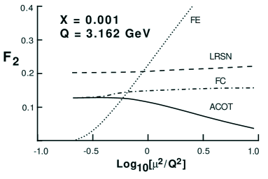
Figure 9: The $\mu$-dependence of $F_{2}(x,Q^{2})$ with $\{x,Q\}=\{10^{-3},3.162\,GeV\}$ for $c$-quark production.

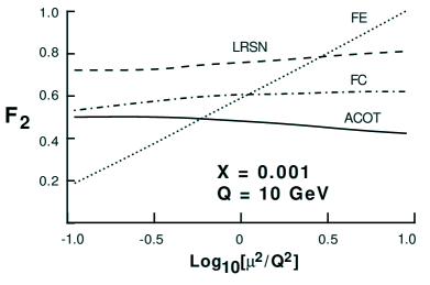
Figure 10: The $\mu$-dependence of $F_{2}(x,Q^{2})$ with $\{x,Q\}=\{10^{-3},10\,GeV\}$ for $c$-quark production.

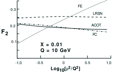
Figure 11: The $\mu$-dependence of $F_{2}(x,Q^{2})$ with $\{x,Q\}=\{10^{-2},10\,GeV\}$ for $c$-quark production.

Figure 12: The $\mu$-dependence of $F_{2}(x,Q^{2})$ with $\{x,Q\}=\{10^{-1},31.62\,GeV\}$ for $c$-quark production.

For $x=0.001$ and $Q=10$ GeV (Figure 10), the ACOT and the LRSN calculations exhibit a comparable and small dependence on the scale choice. In this region, neither is a clear improvement over the FC result.

For $x=0.01$ and $Q=10$ GeV (Figure 11), both the LRSN and ACOT calculations are essentially flat, and both appear to be an improvement over the FC result.

For $x=0.1$ and $Q=31.62$ GeV (Figure 12), the ACOT calculation exhibits slightly less dependence than the LRSN result, and both are considerably less scale-dependent than the FC and FE results.

The general trend revealed here confirms the reduced $\mu$-dependence of the ACOT and LRSN results over their one-order counterparts. Furthermore, we also have confirmation that LRSN is the appropriate calculation near threshold and ACOT in the asymptotic region, as shown when $Q\gg M_{Q}$.

8.2 B-Quark Production

8.2.1 Bottom $F_{2}$ vs. $\{x,Q^{2}\}$

We have also compared the ACOT and the LRSN results for b-quark production. We find very similar features in Figure 13 with $Q=5.623$ GeV for $b$ production as we did in Figure 6 with $Q=1.778$ GeV for $c$. This is as expected since the physics is set by the relevant mass ratio in the process: $M_{Q}/\mu$. The LRSN calculation has a non-trivial K-factor, the FE result essentially vanishes, and the ACOT K-factor is essentially unity.

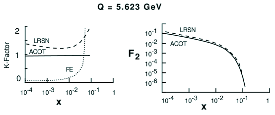
Figure 13: 13a) the K-factor, and 13b) the structure function $F_{2}(x,Q^{2})$ for $b$-production at $Q=5.623GeV$.

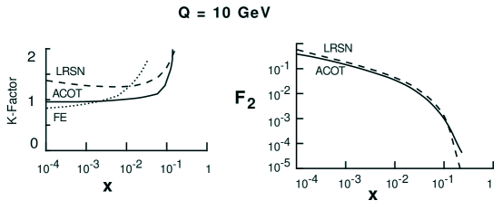
Figure 14: 14a) the K-factor, and 14b) the structure function $F_{2}(x,Q^{2})$ for $b$-production at $Q=10GeV$.

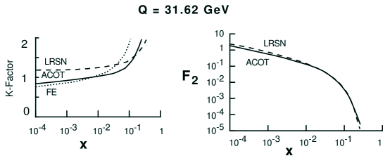
Figure 15: 15a) the K-factor, and 15b) the structure function $F_{2}(x,Q^{2})$ for $b$-production at $Q=31.62GeV$.

For $Q=10$ GeV (Figure 14), the FE results are roughly comparable to the other curves as the heavy-quark evolution turns on. The ACOT K-factor deviates from the FC result as the difference between ${{}^{0}F}_{\scriptscriptstyle V}$ and ${{}^{1s}F}_{\scriptscriptstyle V}$ again signals the existence of non-trivial contributions from the heavy-quark PDF evolution. The LRSN K-factor decreases at small-$x$, and flattens slightly again for the reasons discussed concerning Figure 7.

In Figure 15, we display the results for $Q=31.62$ GeV. The ACOT exhibits a significant difference from the FC process as the heavy-quark evolution continues. As before, the FE, ACOT, and LRSN results have similar shapes, and each K-factor is monotonically increasing as $x$ increases. In the range above $Q=31.62$ GeV, the general characteristics are similar to this figure.

8.2.2 Bottom $F_{2}$ vs. $\mu$

We now examine the $\mu$-dependence of $b$ production at various points in $x$ and $Q^{2}$ space relevant to the region accessible at HERA.

For $x=0.001$ and $Q=10$ GeV (Figure 16), the FE result again has a large $\mu$-dependence because this result is closely tied to $f_{b}(x,\mu)$. The ACOT result is a clear improvement over the FE result, but the FC result exhibits still less dependence and is comparable with the LRSN calculation.

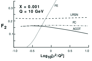
Figure 16: The $\mu$-dependence of $F_{2}(x,Q^{2})$ with $\{x,Q\}=\{10^{-3},10\,GeV\}$ for $b$-quark production.

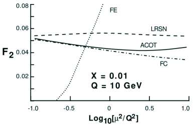
Figure 17: The $\mu$-dependence of $F_{2}(x,Q^{2})$ with $\{x,Q\}=\{10^{-2},10\,GeV\}$ for $b$-quark production.

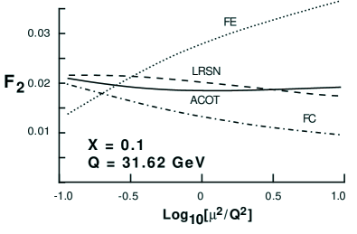
Figure 18: The $\mu$-dependence of $F_{2}(x,Q^{2})$ with $\{x,Q\}=\{10^{-1},31.62\,GeV\}$ for $b$-quark production.

For $x=0.01$ and $Q=10$ GeV (Figure 17), the FE result still has a large $\mu$-dependence, and both the ACOT and the LRSN results improve upon the FC result.

For $x=0.1$ and $Q=31.62$ GeV (Figure 18), the LRSN and the ACOT calculations are comparable and both show substantially less $\mu$-dependence than the FE or FC results.

We can make some general observations regarding the $\mu$-dependence for both charm and bottom production. For all values of $Q$, the FE process is increasing with $\mu$ due to the increasing heavy-quark PDF. In contrast, the ${\cal O}(\alpha_{s}^{1})$ FC process (driven by gluons) is decreasing with $\mu$ largely due to the decrease in $\alpha_{s}(\mu)$. The two-order calculations (ACOT and LRSN) that have compensating contributions to cancel out some of the $\mu$-dependence. Specifically, ACOT combines pieces of the FE and FC processes (together with a subtraction term) to yield a result that has substantially less $\mu$-dependence than either result in the large $Q$ region. LRSN effectively has the ${\cal O}(\alpha_{s}^{2})$ FE contribution as the collinear heavy-quark part of phase space is included, negating some of the $\mu$-dependence of the FC channel.

We note that in general, the ACOT result exhibits minimal $\mu$-dependence at larger values of $Q$ and $x$. At large $Q$, we are closer to the asymptotic region where the VFS approach is expected to be superior. The increased $\mu$-dependence at low $x$ arises mainly from the quark-initated contributions. At a given order, we expect the quark-initiated contributions to be less than the gluon-initiated ones because $f_{q}(x,\mu)\ll f_{g}(x,\mu)$ [4]. However, because the second-order Altarelli-Parisi splitting kernels $P_{q\to q}^{(2)}(x)$ and $P_{g\to q}^{(2)}(x)$ contain singular $1/x$ terms whereas the first-order $P_{q\to q}^{(1)}(x)$ and $P_{g\to q}^{(1)}(x)$ do not, the evolution of the quark distribution at small-$x$ will be completely dominated by the second-order kernel rather than the first-order kernel [12]. Consequently, contributions from higher order quark-initiated processes should cancel the above $\mu$-dependence. This work is in progress [10].

In examining the $\mu$-dependence plots, the reader may have noticed for some $x$ and $Q^{2}$ values chosen, particularly at small $x$, the results of ACOT and LRSN never crossed. The conventional wisdom says the $\mu$-dependence represents the uncertainty from uncalculated higher-order contributions. What are the implications when the $\mu$-dependence curves do not cross when a significant region along the $\mu$-axis has been traversed? At lower values of $Q^{2}$, the difference between ACOT and LRSN is expected due to the limited evolution of the heavy quark PDF. At asymptotic values of $Q^{2}$, the difference between ACOT and LRSN is within the range suggested by the $\mu$ dependence. However, in the intermediate range, the range of the $\mu$-dependence may underestimate the full theoretical uncertainty.

8.2.3 Total Charm and Bottom Cross Section

To estimate the theoretical uncertainty for the total cross section, we have computed

$${}F_{2}(Q^{2})=\int_{10^{-4}}^{x_{max}}dxF_{2}(x,Q^{2})$$ (15)

which is proportional to the dominant contribution for the heavy-quark production cross section and show the ratio of $F_{2}^{ACOT}/F_{2}^{FC}$ and $F_{2}^{LRSN}/F_{2}^{FC}$ for $c$ production in Figure 19. For low $Q$, the differences are on the order of 30%. As $Q$ increases, however, the differences decrease to $\simeq 12\sim 15\%$ as $Q\simeq 100$ GeV. Similar behavior occurs for $b$ production, as seen in Figure 20. Some of this difference may possibly be attributed to choice of scale or PDF set. However variations in scale or PDF set should not be solely responsible for this difference. We may have to await the data from HERA to resolve this discrepancy.

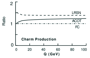
Figure 19: The structure function $F_{2}(Q^{2})$ scaled by the flavor creation (FC) $F_{2}(Q^{2})$ for $c$-quark production. $F_{2}(x,Q^{2})$ has been integrated over $x$ from $x=10^{-4}$ to $x_{max}$ as defined in Equation (15).

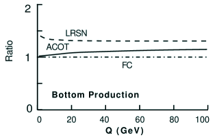
Figure 20: The structure function $F_{2}(Q^{2})$ scaled by the flavor creation (FC) $F_{2}(Q^{2})$ for $b$-quark production. $F_{2}(x,Q^{2})$ has been integrated over $x$ from $x=10^{-4}$ to $x_{max}$ as defined in Equation (15).

9 Conclusions

We have outlined the strengths and weaknesses of both the VFS (ACOT) and the FFS (LRSN) calculation. We summarize the highlights below.

• In the threshold region, the FFS (LRSN) calculation yields the most stable and reliable results due to the domination of flavor creation.

• In the asymptotic region, the VFS (ACOT) calculation provides the best results because of the dominance of the collinear heavy-quark contribution.

• In the kinematic range spanned by HERA, the $\alpha_{s}\log[Q^{2}/M_{Q}^{2}]$ terms are not a significant problem for the FFS (LRSN) calculation.

• In the VFS (ACOT) calculations, the heavy-quark PDF’s can yield significant contributions at relatively small scales, (i.e. $\mu/M_{Q}\sim 3$).

• While the flavor excitation (FE) process can closely match the two-order results with a judicious choice of the scale $\mu$, the large scale dependence makes this unreliable in computing structure functions.

• Likewise, while the flavor creation (FC) process is a good starting point in the threshold region. However, the LRSN calculation indicates that the corrections to this naíve estimate can be as large as 100%.

The range of $x$ and $Q^{2}$ we have presented reflect the region accessible at HERA. We note that the difference between the LRSN and ACOT calculations above threshold is suggestive of higher order contributions yet to be included. As such, the results of this comparison indicate that a combining of the LRSN and ACOT calculations in a consistent fashion (with the additional mass factorizations required) should allow us to make predictions based upon a three-order result that combines the best attributes of both calculations. The result should be a calculation that will provide an important test of perturbative QCD when compared with the results from HERA.

10 Bibliography

References

- [1] A.C. Benvenuti et al., (BCDMS Collaboration), Phys. Letts. B223 (1989) 485; B237 (1990) 592; P. Berge et al., (CDHSW Collaboration), Z. Phys. C35 (1987) 443; P.Z. Quintas et al, CCFR collaboration, Phys. Rev. Letts. 71 (1993) 1307; W.C. Leung, et al., (CCFR Collaboration), Phys. Letts. B317 (1993) 655; J.J. Aubert et al., (EMC Collaboration), Nucl. Phys. B259 (1985) 189; B272 (1986) 158; P. Amaudruz et al., (NMC Collaboration), Phys. Letts. B295 (1992) 159; A. Bodek et al., (SLAC-MIT Collaboration)Phys. Rev. Letts. 50 (1983) 1431; 51 (1983) 534.
- [2] A. Bazarko, et al, (CCFR Collaboration), Nevis R#1502.
- [3] G.A. Schuler, F.I. Olness, J. Blümlein, and W.-K. Tung in Proceedings of the 1990 DPF Summer Study on High Energy Physics: Research Directions for the Decade, Snowmass, CO, p.152, (1992).
-
[4]
M.A.G. Aivazis, F.I. Olness, and W.-K. Tung, SMU-HEP/93-16,
to appear in Phys. Rev. D50, (1994);
M.A.G. Aivazis, J.C. Collins, F.I. Olness and W.-K. Tung, SMU-HEP/93-17, to appear in Phys. Rev. D50, (1994). - [5] J.C. Collins, F. Wilczek, and A. Zee, Phys. Rev. D18, 242 (1978).
- [6] E. Laenen, S. Riemersma, J. Smith, and W.L. van Neerven, Nucl. Phys. B392, 162 (1993).
- [7] E. Laenen, S. Riemersma, J. Smith, and W.L. van Neerven, Nucl. Phys. B392, 229 (1993).
- [8] J.C. Collins, W.-K. Tung Nucl. Phys. B278, 934 (1986).
- [9] Sijin Qian, The CWZ subtraction scheme (A new renormalization prescription for QCD) and its applications, Illinois Inst. of Tech. Ph.D. thesis, UMI-85-17585-mc (microfiche), May 1985.
- [10] P. Agrawal, F.I. Olness, S. Riemersma, and W.-K. Tung, SMU preprint in preparation.
- [11] J. Botts, H.L. Lai, J.G. Morfín, J.F. Owens, J. Qiu, W.-K. Tung and H. Weerts, Version 2 CTEQ Distribution Functions in Parametrized From, MSU preprint in preparation.
- [12] W.-K. Tung, Nucl. Phys. B315, 378 (1989).