TUM-T31-72/94
hep-ph/9408398
August 94
Next-to-leading Order short distance QCD corrections to the effective $\Delta S=2$ Hamiltonian, Implications for the ${\rm K}_{\rm L}$–${\rm K}_{\rm S}$ mass difference

Abstract

We report on the results of a calculation of next-to leading order short distance QCD corrections to the coefficient $\eta_{1}$ of the effective $\Delta S=2$ Lagrangian in the standard model and discuss the uncertainties inherent in such a calculation. As a phenomenological application we comment on the contributions of short distance physics to the ${\rm K}_{\rm L}$–${\rm K}_{\rm S}$ mass difference.

1 Introduction

This report is based on research work done in collaboration with Ulrich Nierste [1].

The prediction of observables in the ${\rm K^{0}}$–$\overline{\rm K^{0}}$ system forces one to calculate an effective low-energy $\Delta S=2$ hamiltonian, which is difficult because of the necessary inclusion of strong interaction effects. Applying Wilson’s operator product expansion factorizes the Feynman amplitude into a long-distance part, to be evaluated by non-perturbative methods, and a short-distance part, which can be calculated in renormalization group improved perturbation theory.

The short distance part of the $\Delta S=2$ Feynman amplitude has first been calculated to leading order (LO) by Vainstein et al. [2], Vysotskij [3] and Gilman and Wise [4]. These determinations leave certain questions unanswered which we like to summarize below. To be specific, consider the effective $\Delta S=2$ hamiltonian

$$H = \frac{{\rm G}_{\rm F}^{2}}{16\pi^{2}}M_{\rm W}^{2}\biggl{[}\lambda_{\rm c}^{2}\eta_{1}S\!\left(\textstyle\frac{m_{\rm c}^{2}}{M_{\rm W}^{2}}\right)+\lambda_{\rm t}^{2}\eta_{2}\times$$ (1)

$$S\!\left(\textstyle\frac{m_{\rm t}^{2}}{M_{\rm W}^{2}}\right)+2\lambda_{\rm c}\lambda_{\rm t}\eta_{3}S\!\left(\textstyle\frac{m_{\rm c}^{2}}{M_{\rm W}^{2}},\frac{m_{\rm t}^{2}}{M_{\rm W}^{2}}\right)\biggr{]}$$

$$\times b\!\left(\mu\right)Q_{\rm LL}\!\left(\mu\right)$$

$$= H^{\rm c}+H^{\rm t}+H^{\rm ct}$$

with ${\rm G}_{\rm F}$ denoting Fermi’s constant, $\lambda_{j}=V_{j{\rm d}}^{*}V_{j{\rm s}}$, $j={\rm c,t}$ the relevant combination of CKM factors and $Q_{\rm LL}$ the local four-quark operator

$$Q_{\rm LL} = \left[\bar{\rm s}\gamma_{\mu}\left(1-\gamma_{5}\right){\rm d}\right]\left[\bar{\rm s}\gamma^{\mu}\left(1-\gamma_{5}\right){\rm d}\right]$$ (2)

In (1) the GIM mechanism $\lambda_{\rm u}+\lambda_{\rm c}+\lambda_{\rm t}=0$ has been used to eliminate $\lambda_{\rm u}$. The Inami-Lim functions $S$ are obtained in the evaluation of the famous box diagrams depicted in fig. 1.

Figure 1: The box diagrams contributing to $H$ in lowest order. The zigzag lines represent ${\rm W}$-bosons or fictitious Higgs particles.

The $\eta_{i}$ parametrize the short distance QCD corrections with their explicit dependence on the renormalization scale $\mu$ factored out in the function $b\!\left(\mu\right)$. In absence of QCD corrections $\eta_{i}b\!\left(\mu\right)=1$.

The LO calculation leaves the following questions unanswered

• The running charm quark mass $m_{\rm c}$ enters (1) at the scale $\mu_{\rm c}\approx m_{\rm c}$, where the dynamic charm quark is removed from the theory. The LO result depends strongly on the choice of $\mu_{\rm c}$. A similar statement applies to the scale $\mu_{\rm W}\approx M_{\rm W}$, where the ${\rm W}$-boson and the top quark are integrated out.

• The precise definition of the QCD scale parameter $\Lambda_{\rm QCD}$ requires at least a next-to-leading order (NLO) calculation.

• Subleading terms may contribute sizeable, e.g. the LO hamiltonian reproduces only about 60% of the observed ${\rm K_{L}}$– ${\rm K_{S}}$ mass difference.

Prior to our work the only part of (1) calculated to NLO was $H^{\rm t}$ containing $\eta_{2}$ [5]. This report deals with $H^{\rm c}$ and the coefficient $\eta_{1}$.

2 The NLO calculation

All calculations are carried out in the $\overline{{\rm MS}}$ scheme using an arbitrary $R_{\xi}$ gauge for the gluon propagator and ’t Hooft–Feynman gauge for the ${\rm W}$-propagator. Inspired by refs. [6, 5] we use an anticommuting $\gamma_{5}$ (NDR scheme). Infrared singularities get regulated by small quark masses. We only calculate the lowest nonvanishing order in $m_{\rm c}/M_{\rm W}$, therefore setting $S\!\left(m_{\rm c}^{2}/M_{\rm W}^{2}\right)=m_{\rm c}^{2}/M_{\rm W}^{2}$. This turns out to be necessary, if we only want to keep operators of the lowest twist.

The calculation is performed in the standard renormalization group technique. The matching of different theories at matching scales $\mu_{\rm W}$, $\mu_{\rm b}$ and $\mu_{\rm c}$ requires the evaluation of the diagram in fig. 2 and diagrams derived from this by dressing it with one gluon in all possible ways.

Figure 2: The lowest order diagram contributing to the effective five and four flavour theories between the scales $\mu_{\rm W}$ and $\mu_{\rm c}$. The crosses denote the insertion of local $\Delta S=1$ operators.

No local $\Delta S=2$ operator appears in the effective five and four quark theory, because the diagrams mentioned above are finite due to the GIM mechanism. Such an operator, it is the $Q_{\rm LL}$ of (2), first arises after moving to an effective three flavour theory by removing the ${\rm c}$-quark. For details, we refer the reader to [1].

To check our calculation, we performed various consistency tests.

• The Wilson coefficient functions turn out to be independent of the gluon gauge parameter $\xi$ and the small quark masses used as a regulator for the infrared singularities.

• Setting $\mu_{\rm W}=\mu_{\rm b}=\mu_{\rm c}$, we recover the result obtained in naive perturbation theory up to the first order in the strong coupling constant $\alpha_{\rm s}$.

• The dependence of the final result on the matching scales $\mu_{\rm W}$, $\mu_{\rm b}$, $\mu_{\rm c}$ vanishes up to first order in $\alpha_{\rm s}$.

3 Numerical results

In the analytical calculation the running charm quark mass renormalized at the scale $\mu_{\rm c}$, where it gets incorporated into the Wilson coefficient function, enters quite naturally. For the numerical analysis and the discussion of renormalization scale dependence it is better to use $m_{\rm c}^{\star}=m_{\rm c}\!\left(m_{\rm c}\right)$. We therefore define $\eta_{1}^{\star}$ by

$$\eta_{1}\!\left(\mu_{\rm W},\mu_{\rm c}\right)m_{\rm c}^{2}\!\left(\mu_{\rm c}\right) = \eta_{1}^{\star}\!\left(\mu_{\rm W},\mu_{\rm c}\right)\left(m_{\rm c}^{\star}\right)^{2}.$$ (3)

In tab. 1 we listed $\eta_{1}^{\star}$ for different values of the QCD scale parameter in the effective four flavour theory $\Lambda_{\overline{\rm MS}}=\Lambda_{4}$ and $m_{\rm c}^{\star}$.

Table 1: $\eta_{1}^{\star}$ for different values of $m_{\rm c}^{\star}$ and $\Lambda_{\overline{\rm MS}}=\Lambda_{4}$ (both given in GeV). The matching scales have been taken to be $\mu_{\rm W}=M_{\rm W}=80{\rm GeV}$, $\mu_{\rm b}=4.8{\rm GeV}$ and $\mu_{\rm c}=m_{\rm c}^{\star}=m_{\rm c}\!\left(m_{\rm c}\right)$.

$\Lambda_{\overline{\rm MS}}$	0.150		0.200		0.250		0.300		0.350
$m_{c}^{\star}$	LO	NLO	LO	NLO	LO	NLO	LO	NLO	LO	NLO
1.25	0.809	0.885	0.895	1.007	0.989	1.154	1.096	1.334	1.216	1.562
1.30	0.797	0.868	0.877	0.982	0.965	1.117	1.064	1.281	1.175	1.485
1.35	0.786	0.854	0.861	0.960	0.944	1.085	1.035	1.235	1.138	1.419
1.40	0.775	0.840	0.847	0.940	0.924	1.056	1.010	1.194	1.105	1.361
1.45	0.766	0.828	0.834	0.922	0.907	1.030	0.987	1.157	1.075	1.310
1.50	0.757	0.817	0.822	0.905	0.890	1.006	0.966	1.125	1.048	1.265
1.55	0.749	0.806	0.810	0.890	0.876	0.985	0.946	1.095	1.024	1.225

Table 2: $\Delta m_{\rm K}^{\rm SD,c}$ in NLO in units of $10^{-15}{\rm GeV}$ for different values of $\Lambda_{\overline{\rm MS}}=\Lambda_{4}$ and $\mu_{\rm c}=m_{\rm c}^{\star}$ (both given in GeV). $B_{\rm K}=0.7$

$\Lambda_{\overline{\rm MS}}$	0.150		0.200		0.250		0.300		0.350
$m_{c}^{\star}$	$\Delta m$	$\frac{\Delta m}{\Delta m_{\rm EXP}}$	$\Delta m$	$\frac{\Delta m}{\Delta m_{\rm EXP}}$	$\Delta m$	$\frac{\Delta m}{\Delta m_{\rm EXP}}$	$\Delta m$	$\frac{\Delta m}{\Delta m_{\rm EXP}}$	$\Delta m$	$\frac{\Delta m}{\Delta m_{\rm EXP}}$
1.25	1.327	0.377	1.510	0.429	1.730	0.491	2.000	0.568	2.342	0.665
1.30	1.408	0.400	1.593	0.452	1.812	0.514	2.078	0.590	2.409	0.684
1.35	1.493	0.424	1.679	0.477	1.897	0.539	2.159	0.613	2.481	0.705
1.40	1.580	0.449	1.768	0.502	1.986	0.564	2.245	0.637	2.560	0.727
1.45	1.670	0.474	1.860	0.528	2.078	0.590	2.335	0.663	2.643	0.751
1.50	1.763	0.501	1.955	0.555	2.173	0.617	2.428	0.689	2.731	0.776
1.55	1.859	0.528	2.052	0.583	2.271	0.645	2.525	0.717	2.824	0.802

For $m_{\rm c}^{\star}=1.4{\rm GeV}$ and $\Lambda_{\overline{\rm MS}}=300{\rm MeV}$ the NLO result is by about 20% larger than the LO one. So the correction turns out to be quite sizable. To estimate something like a “theoretical error”, we look at $\eta_{1}^{\star}$’s dependence on the three matching scales for fixed values of $m_{\rm c}^{\star}$ and $\Lambda_{\overline{\rm MS}}$. The variation with $\mu_{\rm c}$ appears to be the largest one, it is plotted in fig. 3.

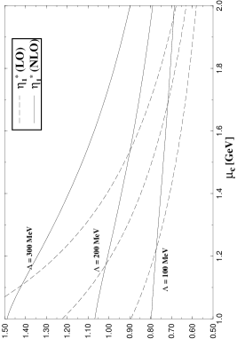
Figure 3: The variation of $\eta_{1}^{\star}$ with the matching scale $\mu_{\rm c}$ for different values of $\Lambda_{\overline{\rm MS}}=\Lambda_{4}$ and $\mu_{\rm c}$. $\mu_{\rm W}=M_{\rm W}=80{\rm GeV}$, $\mu_{\rm b}=4.8{\rm GeV}$ and $m_{\rm c}^{\star}=1.4{\rm GeV}$ have been kept fixed.

It is clearly seen, that the scale dependence in NLO is about 50% smaller than in LO. E.g. for the reference values of $\Lambda_{\overline{\rm MS}}=0.3{\rm GeV}$, $m_{\rm c}^{\star}=1.4{\rm GeV}$, $\mu_{\rm b}=4.8{\rm GeV}$, $\mu_{\rm W}=M_{\rm W}=80{\rm GeV}$ the variation of $\mu_{\rm c}$ from 1.1 to 1.7 GeV amounts to a change of 63% in the LO case and 34% in the NLO result.

$$\eta_{1}^{\star} = 1.01\begin{array}[]{l}\scriptstyle+0.42\\[-5.97508pt] \scriptstyle-0.21\end{array}\mbox{(LO)}$$ (6)

$$\eta_{1}^{\star} = 1.19\begin{array}[]{l}\scriptstyle+0.23\\[-5.97508pt] \scriptstyle-0.17\end{array}\mbox{(NLO)}$$ (9)

Fixing $\mu_{\rm c}=m_{\rm c}^{\star}=1.4{\rm GeV}$, we further analyze the dependence of $\eta_{1}^{\star}$ on the scale $\mu_{\rm W}$. Varying $\mu_{\rm W}$ from 60 to 100 GeV, we find a change of $\eta_{1}^{\star}$ by 7% in LO and 4% in NLO. This residual scale dependence is therefore much weaker than the one for $\mu_{\rm c}$. The residual dependence on the matching scale $\mu_{\rm b}$ turns out to be completely negligible, the extreme choice $\mu_{\rm b}=\mu_{\rm W}=M_{\rm W}$, which means neglecting completely the effects from an effective five flavour theory, leads to an error of the order of 1%.

We now want to discuss the implications of $\eta_{1}^{\star}$ on the short distance contribution to the ${\rm K}_{\rm L}$-${\rm K}_{\rm S}$ mass difference. To a very good approximation the part stemming only from the first two generations is given by [7]

$$\Delta m_{\rm K}^{\rm SD,c} = \frac{{\rm G}_{\rm F}^{2}}{6\pi^{2}}m_{\rm K}f_{\rm K}^{2}B_{\rm K}\left({\rm Re}\lambda_{\rm c}\right)^{2}m_{\rm c}^{\star 2}\eta_{1}^{\star}.$$ (10)

For the input parameters $m_{\rm K}=0.498{\rm GeV}$, $f_{\rm K}=0.161{\rm GeV}$, ${\rm Re}\lambda_{\rm c}=0.215$, ${\rm G}_{\rm F}=1.167\times 10^{-5}{\rm GeV}^{-2}$ and $B_{\rm K}=0.7$ the mass difference $\Delta m_{\rm K}^{\rm SD,c}$ is given in tab. 2. Since $\Delta m_{\rm K}^{\rm SD}$ depends linearly upon the nonperturbative parameter $B_{\rm K}$ the result may be easily rescaled to other values of this parameter. Note, that if we take $\Lambda_{\overline{\rm MS}}=0.3{\rm GeV}$ and $m_{\rm c}^{\star}=1.4{\rm GeV}$, the short distance contribution of the charm sector to the total mass difference is as much as 64%. The terms containing the top quark contribute another 6%, therefore the short distance physics is able to reproduce about 70% of the observed mass difference, which is much more than previously thought.

References

• [1] S.Β Herrlich and U.Β Nierste, Nucl. Phys. B 419 (1994) 292.
• [2] A.Β I. Vainstein, V.Β I. Zakharov, V.Β A. Novikov, and H.Β A. Shifman, Sov. J. Nucl. Phys. 23 (1976) 50.
• [3] M.Β I. Vysotskij, Sov. J. Nucl. Phys. 31 (1980) 797.
• [4] F.Β J. Gilman and M.Β B. Wise, Phys. Rev. D 27 (1983) 1128.
• [5] A.Β J. Buras, M.Β Jamin, and P.Β H. Weisz, Nucl. Phys. B 347 (1990) 491.
• [6] A.Β J. Buras and P.Β H. Weisz, Nucl. Phys. B 333 (1990) 66.
• [7] A.Β J. Buras, W.Β SΕ‚ominski, and H.Β Steger, Nucl. Phys. B 238 (1984) 529.