ANL Preprint Number: PHY-7854-TH-94

Pion Observables and QCD

Craig D. Roberts

Physics Division, Bldg. 203, Argonne National Laboratory,
Argonne, IL 60439-4843, USA

1 Introduction

The Dyson-Schwinger equations (DSEs) are a tower of coupled integral equations that relate the Green functions of QCD to one another. Solving these equations provides the solution of QCD. This tower of equations includes the equation for the quark self-energy, which is the analogue of the gap equation in superconductivity, and the Bethe-Salpeter equation, the solution of which is the quark-antiquark bound state amplitude in QCD. The application of this approach to solving Abelian and non-Abelian gauge theories is reviewed in Ref. 1.

The nonperturbative DSE approach is being developed as both: 1) a computationally less intensive alternative and; 2) a complement to numerical simulations of the lattice action of QCD. In recent years, significant progress has been made with the DSE approach so that it is now possible to make sensible and direct comparisons between quantities calculated using this approach and the results of numerical simulations of Abelian gauge theories.QEDCJB

Herein the application of the DSE approach to the calculation of pion observables is describedCDRpion using: the $\pi$-$\pi$ scattering lengths ($a_{0}^{0}$, $a_{0}^{2}$, $a_{1}^{1}$, $a_{2}^{0}$, $a_{2}^{2}$) and associated partial wave amplitudes; the $\pi^{0}\rightarrow\gamma\gamma$ decay width; and the charged pion form factor, $F_{\pi}(q^{2})$, as illustrative examples. Since this approach provides a straightforward, microscopic description of dynamical chiral symmetry breaking (D$\chi$SB) and confinement, the calculation of pion observables is a simple and elegant illustrative example of its power and efficacy. The relevant DSEs are discussed in Sec. 2, the calculation of pion observables in Sec. 3 and concluding remarks are presented in Sec. 4.

2 Dyson-Schwinger Equations in QCD

2.1 Quark Propagator

In Euclidean space, with metric $\delta_{\mu\nu}=\;{\rm diag}(1,1,1,1)$ and $\gamma_{\mu}=\gamma_{\mu}^{\dagger}$, and in a general covariant gauge, the inverse of the dressed quark propagator can be written as

$$S^{-1}(p)=i\,\gamma\cdot p\,+m+\Sigma(p)\equiv Z^{-1}(p^{2})\left(i\,\gamma\cdot p+M(p^{2})\right)\equiv i\,\gamma\cdot p\,A(p^{2})\,+m+B(p^{2})\/,$$ (2.1)

with: $m$ the renormalised, explicit chiral symmetry breaking mass (if present); $\Sigma(p)$ the self-energy; $M(p^{2})=[m+B(p^{2})]/A(p^{2})$ the dynamical quark mass function; and $Z(p^{2})=A^{-1}(p^{2})$ the momentum-dependent renormalisation of the quark wavefunction. The DSE for the inverse propagator is

$$S^{-1}(p)=i\,\gamma\cdot p+m+\mbox{\small$\displaystyle\frac{4}{3}$}g^{2}\int\frac{d^{4}k}{(2\pi)^{4}}\gamma_{\mu}S(k)\Gamma_{\nu}(k,p)D_{\mu\nu}((p-k)^{2})\/,$$ (2.2)

where $D_{\mu\nu}(q^{2})$ is the dressed gluon propagator and $\Gamma_{\nu}$ is the proper quark-gluon vertex.

When the current-quark mass is zero, the solution of this equation determines whether or not chiral symmetry is dynamically broken in QCD. The quark condensate, $\mbox{$\langle\overline{q}q\rangle$}\propto\mbox{tr$[S(x=0)]$}$, is a chiral symmetry order parameter. If, with $m=0$ in Eq. (2.2), there is a solution with $B\neq 0$ then the quark has generated a mass via interaction with its own gluon field and the chiral symmetry is therefore dynamically broken.

The solution also provides information about quark confinement. The presence or absence of quark production thresholds in the $\cal S$-matrix amplitudes that contribute to physical observables is determined by the analytic structure of the quark propagator, which one obtains by solving this equation.RWK92

2.2 Gluon Propagator

In a general covariant gauge the dressed gluon propagator can be written:

$$D^{\mu\nu}(q^{2})=\left[\left(\delta^{\mu\nu}-\frac{q^{\mu}q^{\nu}}{q^{2}}\right)\frac{1}{1-\Pi(q^{2})}+\xi\frac{q^{\mu}q^{\nu}}{q^{2}}\right]\frac{1}{q^{2}}\/,$$ (2.3)

where $\Pi(q^{2})$ is the gluon vacuum polarisation and $\xi$ is the gauge parameter.

The Dyson-Schwinger equation for the gluon propagator is given diagrammatically in Fig. 1.

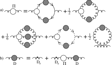
Figure 1: The Dyson-Schwinger equation for the gluon propagator. [Here and below the broken line represents the propagator for the ghost field.]

The symmetrisation factors of 1/2 and 1/6 arise from the usual Feynman rules, which also require a negative sign [unshown] to be included for every fermion and ghost loop. This equation has been studied extensively.SM79 ; UBG80 ; BBZBP ; H90b There have also been attempts to determine the gluon propagator from numerical simulations of lattice-QCD.MO ; BPS94

The results of the DSE and lattice studies are summarised in Sec. 5.1 of Ref. 1 and are represented in Fig. 2.

Figure 2: Results of studies of the gluon propagator in QCD. Typical values of $m_{g}=0.5$ GeV and $b=0.7$ GeV have been used.

This figure illustrates that for spacelike-$q^{2}>1$ GeV² the gluon propagator is given by the two-loop, QCD renormalisation group result, with the next order correction being $<$10%. For spacelike-$q^{2}<1$ GeV², however, the form of the propagator is not known.

The DSE studies of Refs. 5; 6; 7 suggest a regularised infrared singularity, represented by $1/q^{4}$ in the figure. That of Ref. 8, which differs mainly in that the Ansatz used for the triple-gluon vertex has kinematic singularities, suggests an infrared vanishing form, characterised by $q^{2}/(q^{4}+b^{4})$, which has also been arguedVG79Zw91 to be the form necessary to completely eliminate Gribov copies.

The lattice Landau-gauge simulations of Ref. 9 favour the massive vector boson form, $1/(q^{2}+m_{g}^{2})$, which is broadly consistent with the improved simulations of Ref. 10. In some cases, however, these improved simulations allowed a fit of the form $q^{2}/(q^{4}+b^{4})$, with $b\sim 340$ MeV. There is a problem with lattice simulations, however, indicated by the dashed vertical line at the right of Fig. 2. With present technology, the domain of $q^{2}<1$ GeV² is actually inaccessible in lattice studies and, since all forms of the propagator are the same outside this domain, it is clear that these results are both qualitatively and quantitatively unreliable.

2.3 Bound States: Bethe-Salpeter Equation

In quantum field theory, the Bethe-Salpeter amplitude for a two-body, quark-antiquark bound state is obtained as the solution of the homogeneous Bethe-Salpeter equation:

$$\Gamma^{rs}_{M}(p;P)=-\int\,\mbox{\small$\displaystyle\frac{d^{4}k}{(2\pi)^{4}}$}\,K^{rs;tu}_{ab;cd}(k,p;P)\,\left(S(k-\mbox{\small$\displaystyle\frac{1}{2}$}P)\Gamma_{M}(k;P)S(k+\mbox{\small$\displaystyle\frac{1}{2}$}P)\right)^{tu}_{cd},$$ (2.4)

where $\Gamma_{M}$ is the proper meson-quark vertex and $K$ is the kernel. A commonly used approximation for the kernel, $K$, is generalised ladder approximation, in which

$$K=g^{2}\,D_{\mu\nu}(p-q)\,\left(\frac{\lambda^{a}}{2}\right)_{ac}\left(\frac{\lambda^{a}}{2}\right)_{db}\left(\gamma_{\mu}\right)_{rt}\left(\gamma_{\mu}\right)_{us}$$ (2.5)

and $S(k)$ is obtained from the rainbow approximation to the quark DSE; i.e., Eq. (2.2) with $\Gamma_{\mu}=\gamma_{\mu}$. Solving for $\Gamma_{M}$ in this approximation yields what is meant by the dressed-quark core of the bound state.

In the DSE approach the dichotomy of the pion as both a Goldstone boson and a $q$-$\bar{q}$ bound state is beautifully and easily understood. One has D$\chi$SB when, with $m=0$ in Eq. (2.2), one obtains $B_{m=0}(p^{2})\neq 0$ as a solution. In this case $(m=0)$ the Bethe-Salpeter equation in the pseudoscalar channel reduces to the quark DSE as $P^{2}\rightarrow 0$, where $P_{\mu}$ is the centre-of-mass momentum of the bound state.DS79 It follows without fine-tuning, therefore, that if the quark DSE admits $B_{m=0}(p^{2})\neq 0$ as a solution when $m=0$; i.e., one has D$\chi$SB, then there exists a massless $(P^{2}=0)$, pseudoscalar, $q$-$\bar{q}$ bound state with the proper meson-quark vertex dominated by its $\gamma_{5}$ component; i.e., $\Gamma_{\pi}(p^{2};P^{2}=0)=B_{m=0}(p^{2})/f_{\pi}$, where $f_{\pi}$ is both the Bethe-Salpeter normalisation and pion decay constant, which is a calculated quantity in this approach. For $m\neq 0$ but $m/\Lambda_{\rm QCD}\ll 1$ one has

$$\Gamma_{\pi}(p^{2};P^{2}=-m_{\pi}^{2}) \approx \frac{1}{f_{\pi}}B_{m=0}(p^{2})$$ (2.6)

$$m_{\pi}^{2}f_{\pi}^{2} \approx 2m\langle\bar{q}q\rangle.$$ (2.7)

2.4 Solution of the Quark Dyson-Schwinger Equation

The DSE for the quark propagator, Eq. (2.2), has been much studied (see Sec. 6 of Ref. 1). The numerical solution obtained using a gluon propagator with an integrable singularity in the infrared region (upper curve in Fig. 2) and a quark-gluon vertex of the Ball-Chiu typeBC80 can be represented well by the following algebraic parametrisation:CDRpion

$$\bar{\sigma}_{S}(x)=Ce^{-2x}+$$

$$\frac{1-e^{-b_{1}x}}{b_{1}x}\,\frac{1-e^{-b_{3}x}}{b_{3}x}\,\left(b_{0}+b_{2}\frac{1-e^{-\Lambda x}}{\Lambda\,x}\right)+\frac{\bar{m}}{x+\bar{m}^{2}}\left(1-e^{-2\,(x+\bar{m}^{2})}\right)$$

$$\bar{\sigma}_{V}(x)=\frac{2(x+\bar{m}^{2})-1+e^{-2(x+\bar{m}^{2})}}{2(x+\bar{m}^{2})^{2}}-\bar{m}Ce^{-2x},$$ (2.9)

where $S(p)=-i\gamma\cdot p\,\sigma_{V}(p^{2})+\sigma_{S}(p^{2})$, $x=p^{2}/(2D)$, $\bar{\sigma}_{S}(x)=\sqrt{2D}\sigma_{S}(p^{2})$, $\bar{\sigma}_{V}(x)=(2D)\sigma_{V}(p^{2})$, $\bar{m}=m/\sqrt{2D}$, and $D$ sets the mass scale. This parametrisation provides a representation of the quark propagator that is an entire function in the complex $p^{2}$ plane but for an essential singularity, as suggested by Ref. 15, which is sufficient to ensure confinement.

Equations (2.4) and (2.9) provide a six parameter algebraic approximation to the quark propagator in QCD: $C$, $\bar{m}$, $b_{0},\ldots,b_{3}$. [$\Lambda(=10^{-4})$ simply decouples $b_{2}$ from the quark condensate.] The parameters can be chosen so as to provide an accurate approximation to a numerical solution of Eq. (2.2). However, as illustrated in Fig. 2, the form of the gluon propagator for $q^{2}<1$ GeV² is unknown. This parametrisation is therefore also an implicit parametrisation of the gluon propagator in this region. Using this quark propagator to calculate experimental observables, and choosing the parameters so as to obtain the best possible fit to these observables, one has a direct connection between observables and the form of the effective quark-quark interaction in the infrared. This provides a means for using precise, low-energy experimental data to determine the effective quark-quark interaction in the infrared.

3 Calculating Pion Observables

In much the same way as an effective action can be used to formalise the constraints of chiral Ward identities in QCD, one can formalise the Abelian approximation to QCD (which decouples the ghost fields and reduces the Slavnov-Taylor identities to Ward identities; see Ref. 6 and Sec. 5 of Ref. 1) via a model field theory described by the action:CR85

$$S[\bar{q},q]=\int\,d^{4}x\,d^{4}y\,\left\{\bar{q}(x)\left[\gamma\cdot\partial+m\right]\delta^{4}(x-y)q(y)+\frac{1}{2}j^{a}_{\mu}(x)g^{2}D_{\mu\nu}(x-y)j_{\nu}^{a}(y)\right\}$$ (3.1)

with $j_{\mu}^{a}(x)=\bar{q}(x)\,\left(\lambda^{a}/2\right)\,\gamma_{\mu}q(x)$ and $D_{\mu\nu}$ the gluon propagator. This model field theory is called the Global Colour-symmetry Model (GCM).

3.1 $\pi$-$\pi$ Scattering

The $\pi$-$\pi$ scattering $T$-matrix is completely specified by one scalar function, $A(s,t,u)$:

$$T_{\alpha\beta;\gamma\delta}=A(s,t,u)\,\delta_{\alpha\beta}\delta_{\gamma\delta}+A(t,s,u)\,\delta_{\alpha\gamma}\delta_{\beta\delta}+A(u,t,s)\,\delta_{\alpha\delta}\delta_{\beta\gamma}~{}.$$ (3.2)

In the DSE-GCM approach the tree-level contribution to $A(s,t,u)$ is obtained from a sum of intrinsically-finite quark-loop diagrams, which, using Eqs. (2.4) and (2.9), have no quark production thresholds. Although it is not necessary, one can perform a derivative expansion of this sum of quark-loop contributions to obtain:RCSI94

$$A(s,t,u)=\frac{m_{\pi}^{2}+2\,s-t-u}{3\,f_{\pi}^{2}}+\frac{4N_{c}}{3f_{\pi}^{4}}\times$$

$$\left[\rule{0.0pt}{11.38109pt}K_{1}\left(-12\,{m_{\pi}^{4}}+6\,{m_{\pi}^{2}}\,(s+t+u)+2\,{s^{2}}-{t^{2}}-{u^{2}}-2(\,s\,t+\,s\,u+\,t\,u)\right)\right.$$

$$+K_{2}\left.\left(-2\,{m_{\pi}^{2}}+s\right)\,\left(-2\,{m_{\pi}^{2}}+t+u\right)+K_{3}\left(-2\,{m_{\pi}^{4}}+{m_{\pi}^{2}}\,(s+t+u)-t\,u\right)\rule{0.0pt}{11.38109pt}\right],$$

$$\mbox{where}\;f_{\pi}^{2}=\frac{N_{c}}{8\pi^{2}}\int_{0}^{\infty}\,ds\,s\,B_{m\neq 0}^{2}\,\times$$

$$\left(\sigma_{V}^{2}-2\left[\sigma_{S}\sigma_{S}^{\prime}+s\sigma_{V}\sigma_{V}^{\prime}\right]-s\left[\sigma_{S}\sigma_{S}^{\prime\prime}-\left(\sigma_{S}^{\prime}\right)^{2}\right]-s^{2}\left[\sigma_{V}\sigma_{V}^{\prime\prime}-\left(\sigma_{V}^{\prime}\right)^{2}\right]\right)~{},$$

and $m_{\pi}$ is obtained from Eq. (2.7) with

$$-\langle\bar{q}q\rangle_{\mu}=$$

$$\left(\ln\frac{\mu^{2}}{\Lambda_{QCD}^{2}}\right)^{\alpha}\lim_{\Lambda_{UV}^{2}\rightarrow\infty}\left(\ln\frac{\Lambda_{UV}^{2}}{\Lambda_{QCD}^{2}}\right)^{-\alpha}\frac{3}{4\pi^{2}}\int_{0}^{\Lambda_{UV}^{2}}\,ds\,s\left(\sigma_{S}(s)-\frac{m}{s+m^{2}}\right)~{}.$$

The constants $K_{i}$ are also given by one dimensional integrals whose integrands involve only the quark propagator.RCSI94 Clearly, and importantly, each of the quantities appearing in Eq. (3.1) is determined once the quark propagator is specified. The utility of the derivative expansion is only that it facilitates a comparison with other calculations of $A(s,t,u)$.

3.2 $\pi^{0}\rightarrow\gamma\gamma$

In Euclidean metric the matrix element for the decay $\pi^{0}\rightarrow\gamma\gamma$ can be written

$${\cal M}(k_{1},k_{2})=-2\,i\,\frac{\alpha_{em}}{\pi f_{\pi}}\,\epsilon_{\mu\nu\rho\sigma}\epsilon_{\mu}(k_{1})\,\epsilon_{\nu}(k_{2})\,k_{1\rho}\,k_{2\sigma}\,G(k_{1}\cdot k_{2})~{},$$ (3.6)

where $k_{i}$ are the photon momenta and $\epsilon(k_{i})$ are their polarisation vectors. Here, the $\pi^{0}$ momentum is $P=(k_{1}+k_{2})$ and $P^{2}=2\,k_{1}\cdot k_{2}$.

Using Eq. (3.6) one finds easily that $\Gamma_{\pi^{0}\rightarrow\gamma\gamma}=[m_{\pi}^{3}\alpha_{em}^{2}G(-m_{\pi}^{2})^{2}]/[16\pi^{3}f_{\pi}^{2}]$. Experimentally one has $\Gamma_{\pi^{0}\rightarrow\gamma\gamma}=(7.74\pm 0.56)~{}\mbox{eV}$, which corresponds to

$$g_{\pi^{0}\gamma\gamma}\equiv G(-m_{\pi}^{2})=0.504\pm 0.019~{},$$ (3.7)

using $m_{\pi^{0}}=135$ MeV and $f_{\pi}=93.1$ MeV.

In generalised impulse approximation $g_{\pi^{0}\gamma\gamma}$ is obtained from the sum of two quark-loop diagrams and, in the chiral limit $(P^{2}=0)$, one has:CDRpion

$$g_{\pi^{0}\gamma\gamma}^{0}\equiv G(0)=\int_{0}^{\infty}\,ds\,s\,B_{m=0}\,A\,\sigma_{V}\,\times$$

$$\left\{\rule{0.0pt}{11.38109pt}A\,\left[\sigma_{V}\,\sigma_{S}+s\left(\sigma_{V}^{\prime}\,\sigma_{S}-\sigma_{V}\,\sigma_{S}^{\prime}\right)\right]+s\,\sigma_{V}\,\left(A^{\prime}\,\sigma_{S}-B^{\prime}\sigma_{V}\right)\right\}~{}.$$

Defining $C(s)=B_{m=0}(s)^{2}/[s\,A(s)^{2}]$ one obtains a dramatic simplification and, because of D$\chi$SB; i.e., because $f_{\pi}\Gamma_{\pi}=B_{m=0}$,

$$g_{\pi^{0}\gamma\gamma}^{0}=\int_{0}^{\infty}\,dC\,\frac{1}{(1+C)^{3}}=\frac{1}{2}~{},$$ (3.9)

since $C(s=0)=\infty$ and $C(s=\infty)=0$. Hence, the experimental value is reproduced, independent of the details of $S(p)$. This illustrates the manner in which the Abelian anomaly is incorporated in the DSE framework. This result will be violated in any approach that does not properly incorporate D$\chi$SB; i.e., in any approach which violates the chiral-limit identity: $f_{\pi}\,\Gamma_{\pi}=B_{m=0}$.

3.3 $F_{\pi}(q^{2})$

In generalised impulse approximation, in Euclidean metric, with $\gamma_{\mu}$ hermitian, the $\pi$-$\pi$-$\gamma$ vertex isCDRpion

$$\Lambda_{\mu}(P+q,-P)=\frac{N_{c}}{f_{\pi}^{2}}\,\int\mbox{\small$\displaystyle\frac{d^{4}k}{(2\pi)^{4}}$}\,$$

$${\rm tr}_{D}\left[i\overline{\Gamma}_{\pi}(k;P+q)S(k_{++})i\Gamma_{\mu}^{\rm BC}(k_{++},k_{-+})S(k_{-+})i\Gamma_{\pi}(k-\mbox{\small$\displaystyle\frac{1}{2}$}q;-P)S(k_{--})\right],$$

where $q$ is the photon momentum, $P$ is the initial momentum of the pion,$k_{\alpha\beta}=k+\mbox{\small$\displaystyle\frac{\alpha}{2}$}q+\mbox{\small$\displaystyle\frac{\beta}{2}$}P$ andBC80

$$\Gamma_{\mu}^{\rm BC}(p,q)=\Sigma_{A}(p,q)\,\gamma_{\mu}+(p+q)_{\mu}\left\{\Delta_{A}(p,q)\,\mbox{\small$\displaystyle\frac{1}{2}$}\,\left[\gamma\cdot p+\gamma\cdot q\right]-i\Delta_{B}(p,q)\right\}$$ (3.11)

with $\Sigma_{H}(p,q)\equiv[H(p^{2})+H(q^{2})]/2$ and $\Delta_{H}(p,q)\equiv[H(p^{2})-H(q^{2})]/[p^{2}-q^{2}]$, for $H=A$ or $B$. $\Gamma_{\mu}^{\rm BC}$ satisfies the Ward-Takahashi identity and ensures the conservation of the pion currentCDRpion so that $\Lambda_{\mu}(P+q,-P)$$=(2P_{\mu}+q_{\mu})F_{\pi}(q^{2})$.

3.4 Fitting the Parameters and Calculated Results

The parameters in Eqs. (2.4) and (2.9) are fixed by requiring a global best-fit to:

$$\begin{array}[]{ccc}\displaystyle\frac{f_{\pi}}{\langle\overline{q}q\rangle^{\frac{1}{3}}}=0.423\pm 0.024~{},&\;\;f_{\pi}\,r_{\pi}=0.318\pm 0.006~{},\;\;\displaystyle\frac{m_{\pi}^{2}}{\langle\overline{q}q\rangle^{\frac{2}{3}}}=0.396\pm 0.036~{};\end{array}$$ (3.12)

the dimensionless $\pi$-$\pi$ scattering lengths

$$\begin{array}[]{ll}a_{0}^{0}=0.21\pm 0.02~{},&a_{0}^{2}=-0.040\pm 0.003~{},\\ a_{1}^{1}=0.038\pm 0.002~{},&a_{2}^{0}=0.0017\pm 0.0003~{};\end{array}$$ (3.13)

and a least-squares fit to $F_{\pi}(q^{2})$ on the spacelike-$q^{2}$ domain: $[0,4]$ GeV². The fitting procedure used $f_{\pi}$ from Eq. (3.1) and $\langle\bar{q}q\rangle$ from Eq. (3.1), with $\Lambda_{QCD}=0.20$ GeV and $\alpha=1$ [not the true anomalous dimension because $\ln[p^{2}]$-corrections have not been included in Eqs. (2.4) and (2.9)] and the expressions for $a_{0}^{0}$, $a_{0}^{2}$, $a_{1}^{1}$, $a_{2}^{0}$ and $r_{\pi}$ given in Ref. 16. It yielded

$$\begin{array}[]{cc}C=0.0406~{},&\overline{m}=0.0119~{},\end{array}$$ (3.15)

$$\begin{array}[]{cccc}b_{0}=0.118~{},&b_{1}=2.51~{},&b_{2}=0.525~{},&b_{3}=0.169~{}.\end{array}$$ (3.17)

The mass scale is set by requiring equality between the percentage error in $f_{\pi}$ and $r_{\pi}$, which yields $D=0.133$ GeV².

The low-energy physical observables calculated with this parameter set are compared with their physical values in Table 1, where $m^{\rm ave}=\left(m_{u}+m_{d}\right)/2$ and the “experimental” value of $\langle\bar{q}q\rangle^{\frac{1}{3}}$ is that typically used in QCD sum rules analysis. The calculated quantities were evaluated at the listed value of $m_{\pi}$; i.e., the chiral limit expressions were not used, but the corrections are $<1$% in each case. The agreement is excellent.

	Calculated	Experiment
$f_{\pi}\;$	0.0839 GeV	0.0931 $\pm$ 0.001
$-\langle\bar{q}q\rangle^{\frac{1}{3}}_{1\,{\rm GeV}^{2}}$	0.211	0.220 $\pm$ 0.01
$m^{\rm ave}_{1\,{\rm GeV}^{2}}$	0.0061	0.0075 $\pm$ 0.004
$m_{\pi}\;$	0.127	0.138
$r_{\pi}\;$	0.596 fm	0.663$\pm$ 0.006
$g_{\pi^{0}\gamma\gamma}\;$	0.497 (dimensionless)	0.504 $\pm$ 0.019
$a_{0}^{0}\;$	0.174	0.21$\pm$0.02
$a_{0}^{2}\;$	-0.0496	-0.040 $\pm$ 0.003
$a_{1}^{1}\;$	0.0307	0.038 $\pm$ 0.002
$a_{2}^{0}\;$	0.00161	0.0017 $\pm$ 0.0003
$a_{2}^{2}\;$	-0.000251

Table 1: Comparison of tree-level DSE calculations with experiment.

The $\pi$-$\pi$ partial wave amplitudes associated with $a_{0}^{0}$ and $a_{0}^{2}$, calculated using the formulae in Ref. 16, are plotted in Fig. 3 and can be seen to be in agreement with the data up to $x\approx 3$, which corresponds to $E\approx 4m_{\pi}$. The same is true of the higher partial wave amplitudes.CDRpion

Figure 3: Partial wave amplitudes in $\pi$-$\pi$ scattering ($x=E^{2}/(4m_{\pi}^{2})-1$): solid line - this calculation; dashed line - current algebra.SW66

The calculated form of $F_{\pi}(q^{2})$ is presented in Fig. 4 and, given that the extraction of the “experimental” point at $q^{2}=6.3$ GeV², measured in pion electroproductionExp78 is strongly model dependent, the agreement with the experimental data is again excellent.

Figure 4: Calculated form of $F_{\pi}(q^{2})$. The experimental data are from Refs.18 (crosses), 19 (diamonds) and 20 (circles).

4 Concluding Remarks

In principle, QCD can be solved using the Dyson-Schwinger equation (DSE) framework, however, in practice, obstacles to achieving this goal remain. The successes and remaining challenges are discussed in detail in Ref. 1.

Herein, the practical application of the DSE approach to the calculation of physical observables is illustrated. By its very nature, the approach directly incorporates all of the known large spacelike-$q^{2}$ behaviour of QCD. It has a phenomenological, model dependent aspect that is tied to the fact that the gluon propagator, $D_{\mu\nu}(q)$, is unknown for spacelike-$q^{2}<1$ GeV². This has the benefit that, in calculating experimental observables in this approach, one obtains a representation of these observables in terms of the infrared structure of $D_{\mu\nu}(q)$ and can thereby use precision experimental measurements to determine the infrared form of the gluon propagator.

In the DSE approach the pion has an intrinsic size; i.e., it is not pointlike, and its dominant determining characteristic is its dressed quark core, which is described by the proper pion-quark vertex function in Eq. (2.6). The calculations reported herein are tree-level calculations, which here actually means that they are obtained with the minimal number of dressed-quark loops. The agreement between theory and experiment is at the 10% level, which is consistent with Refs. 21; 22 where nonpointlike $\pi$-loop contributions are shown to provide $<15$% corrections.

Low Energy Constant	tree-level DSE	1-$\rule{0.0pt}{10.0pt}\pi^{\rm point}$-loop ChPTGL84
$\rule{0.0pt}{10.0pt}\bar{\ell}_{1}$	$-6.1$	$-2.3\pm 3.7$
$\rule{0.0pt}{10.0pt}\bar{\ell}_{2}$	$~{}6.6$	$~{}6.0\pm 1.3$
$\rule{0.0pt}{10.0pt}\bar{\ell}_{6}$	$11.7$	$16.5\pm 1.1$

Table 2: Low-energy constants of ChPT inferred from tree-level DSE calculations of experimental observables.

Clearly, experimental observables can be calculated directly in the DSE approach. From these calculations, however, one might infer values of the low-energy constants used in Chiral Perturbation Theory (ChPT) to parametrise the solution of the chiral Ward identities in QCD. This will provide implicit, nonlinear relations between these constants and the few, underlying parameters of QCD. The results inferred for $\bar{\ell}_{1}$, $\bar{\ell}_{2}$ and $\bar{\ell}_{6}$ from DSE-tree-level calculations are presented in Table. 2 and compared with the 1-point-pion-loop corrected values used in ChPT. (The 1-nonpointlike-pion-loop correction to $r_{\pi}$ estimated in Ref. 22 yields $\bar{\ell}_{6}\simeq 13.0-13.5$.) This comparison indicates that tree-level DSE calculations incorporate those effects of point-pion-loops in ChPT that serve merely to mock-up the pion’s internal structure. Calculations from which the value of other of these constants can be inferred are underway.ICDRT

Acknowledgments. I would like to thank and congratulate the organisers, Aron Bernstein and Barry Holstein, for bringing about this timely and stimulating meeting, and the workshop secretary, Joanne Gregory, for ensuring that it ran smoothly. This work was supported by the Department of Energy, Nuclear Physics Division under contract number W-31-109-ENG-38.

References

- (1) C. D. Roberts and A. G. Williams: Dyson-Schwinger Equations and their Application to Hadronic Physics, in Progress in Particle and Nuclear Physics, Vol. 33, pp. 477-575, ed. by A. Fäßler (Pergamon Press, Oxford, 1994).
- (2) C. J. Burden: How can QED3 help us understand QCD4, in Proceedings of “The Workshop on QCD Vacuum Structure”, American University of Paris, 1-5 June 1992, Editors H. M. Fried and B. Müller (World Scientific, New York, 1993).
- (3) C. D. Roberts: Electromagnetic pion form factor and neutral pion decay, Argonne National Laboratory preprint # PHY-7842-TH-94 (1994).
- (4) C. D. Roberts, A. G. Williams and G. Krein: Int. J. Mod. Phys. A 7 5607 (1992)
- (5) S. Mandelstam: Phys. Rev. D20 3223 (1979)
- (6) U. Bar-Gadda: Nucl. Phys. B163 312 (1980)
- (7) M. Baker, J. S. Ball and F. Zachariasen: Nucl. Phys. B186 531,560 (1981); B226 455 (1983); N. Brown and M. R. Pennington: Phys. Lett. B202 257 (1988); Phys. Rev. D38 2266 (1988)
- (8) U. Häbel, et al: Z. Phys. A336 423, 435 (1990)
- (9) J. E. Mandula and M. Ogilvie: Nucl. Phys. B1A (Proc. Suppl.) 117 (1987); Phys. Lett. B185 127 (1987)
- (10) C. Bernard, C. Parrinello and A. Soni: Phys. Rev. D 49 1585 (1994)
- (11) V. N. Gribov: Nucl. Phys. B 139 1 (1979); D. Zwanziger, Nucl. Phys. B364 127 (1991)
- (12) J. S. Ball and T.-W. Chiu: Phys. Rev. D22 2542 (1980)
- (13) R. Delbourgo and M. D. Scadron: J. Phys. G 5 1631 (1979)
- (14) R. T. Cahill and C. D. Roberts: Phys. Rev. D 32 2419 (1985)
- (15) C. J. Burden, C. D. Roberts and A. G. Williams: Phys. Lett. B285 347 (1992)
- (16) C. D. Roberts, R. T. Cahill, M. E. Sevior and N. Iannella: Phys. Rev. D 49 125 (1994)
- (17) S. Weinberg: Phys. Rev. Lett. 17 616 (1966).
- (18) C. N. Brown: et al, Phys. Rev. D 8 92 (1973)
- (19) C. J. Bebek: et al, Phys. Rev. D 13 25 (1976)
- (20) C. J. Bebek: et al, Phys. Rev. D 17 1693 (1978)
- (21) L. C. L. Hollenberg, C. D. Roberts and B. H. J. McKellar: Phys. Rev. C 46, 2057 (1992)
- (22) R. Alkofer, A. Bender and C. D. Roberts: Pion Loop Contribution to the Electromagnetic Pion Charge Radius, ANL preprint # PHY-7663-TH-93 (1993)
- (23) J. Gasser and H. Leutwyler: Ann. Phys. (NY) 158 142 (1984)
- (24) I. Chappell: A Calculation of the Pion Scalar Radius, Argonne National Laboratory DEP report (1994); A. J. Davies, C. D. Roberts and M. J. Thomson: in progress.