Colored Chaos

Abstract

I review recent progress in our understanding of the basis of statistical models for hadronic reactions and of the mechanisms of thermalization in nonabelian gauge theories.

Almost to the date 30 years ago, Rolf Hagedorn proposed:$\sevenrm^{\hbox{\immediate{?}}}$ that multiparticle production and other phenomena of what today is called “soft” hadronic interactions could be explained on the basis of two assumptions

1. The mass spectrum of hadronic states grows as $\rho(m)\sim m^{-a}\;e^{bm}$.

2. The available states are statistically occupied during a (soft) hadronic interaction.

We now understand that the first assumption, an exponentially growing mass spectrum, is a consequence of quark confinement, and the famous Hagedorn temperature $T_{H}=1/b$ is related to the QCD string tension and the temperature $T_{c}$ associated with the deconfining, chiral symmetry restoring phase transition of QCD.

The second assumption has remained more mysterious. Why is the assumption of a random statistical distribution of final states warranted in high energy reactions that last not much longer than 1 fm/c (or $3\times 10^{-24}$s), and why are the final states not dominated by coherent quantum states or collective excitations of a small subset of the available hadronic degrees of freedom? Maybe it is good to recall that similar questions posed themselves in the context of Bohr’s statistical model of compound nucleus reactions. In this case, the conceptual difficulties were eventually resolved by the insight that the highly excited compound nucleus is a chaotic quantum system $\sevenrm^{\hbox{\immediate{?}}}$ exhibiting rapid exchange of energy between the accessible degrees of freedom. Here I want to show that the same mechanism is responsible for the apparent thermalization in high-energy hadron-hadron interactions: nonabelian gauge theories are strongly chaotic.

Chaos and Ergodicity

A dynamical system exhibits ergodic behavior, if the time average of an observable $A$ can be replaced by the phase space average

$$\lim_{T\to\infty}{1\over T}\int_{0}^{T}dtA(t)=\langle A\rangle\equiv{1\over Z_{E}}\int d\Gamma_{E}A(\Gamma_{E}).$$ (1)

$\langle A\rangle$ here denotes the microcanonical average, $Z_{E}$ is the microcanonical partition function, and $d\Gamma_{E}$ is the phase space measure at constant energy. For systems with very many degrees of freedom it is equivalent to take the canonical average

$$\langle A\rangle={1\over Z(\beta)}\int d\Gamma A(\Gamma)\exp[-\beta E(\Gamma)],$$ (2)

where $Z(\beta)=\int d\Gamma\exp[-\beta E(\Gamma)]$ is the canonical partition function and the inverse temperature $\beta=1/T$ is determined by the condition $E=-\partial(\ln Z)/\partial\beta$.

For practical applications it is crucial to know the time scale on which ergodicity is attained. It can be shown that this time scale is related to the rate $h$ of exponential divergence of neighboring trajectories in phase space; this rate is called the (maximal) Lyapunov exponent .$\sevenrm^{\hbox{\immediate{?}}}$ The complete spectrum of Lyapunov exponents is defined as follows. Consider a given trajectory in phase space, $x_{\alpha}(t)$, where $\alpha=1,\ldots\nu$ enumerates the degrees of freedom. $x_{\alpha}(t)$ is a solution of the classical equations of motion of the system. Now take a set of neighboring trajectories (see Figure 1):

$$\tilde{x}_{\alpha}^{\prime(i)}(t)=x_{\alpha}(t)+\delta x_{\alpha}^{(i)}(t),\quad\alpha=1,\ldots,\nu.$$ (3)

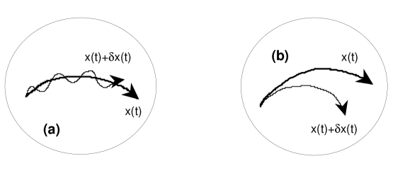
Figure 1: (a) Stable phase space trajectory; (b) unstable trajectory.

For infinitesimal $\delta x_{\alpha}$ they are solutions of a second-order linear differential equation of the form

$$D[x_{\alpha}(t)]\delta x_{\alpha}^{(i)}(t)=0.$$ (4)

One can then obtain a complete orthogonal set of solutions of this equation; they define $\nu$ Lyapunov exponents $\lambda_{i}$ according to

$$\lambda_{i}=\lim_{t\to\infty}{1\over t}\ln{\|\delta x_{\alpha}^{(i)}(t)\|\over\|\delta x_{\alpha}^{(i)}(0)\|},\quad i=1,\ldots,\nu.$$ (5)

In other words, for long times one has the norm of $\delta x_{\alpha}^{(i)}$ growing (or shrinking) as $\|\delta x_{\alpha}^{(i)}(t)\|\propto\exp(\lambda_{i}t)$. One usually assumes the Lyapunov exponents to the ordered in size:

$$\lambda_{1}\equiv h\geq\lambda_{2}\geq\ldots\geq\lambda_{\nu}.$$ (6)

For conservative (Hamiltonian) systems the Lyapunov exponents occur in pairs of equal size, but opposite sign: $\lambda_{i}=-\lambda_{N+1-i}$. This is in accordance with Liouville’s theorem which states that the volumes in phase space filled by an ensemble remains unchanged with time, implying that there must be a direction of contraction for every direction in which the phase space volume expands. For each conservation law there occur two vanishing Lyapunov exponents; the conservation of energy always ensures the existence of one such pair for a Hamiltonian system. Since the extent of the ensemble rapidly shrinks below any practially achievable resolution in the exponentially contracting directions, the observable volume in phase space grows as

$$\overline{\Gamma}(t)\propto\exp\left(t\sum_{i}\lambda_{i}\theta(\lambda_{i})\right)\equiv\exp(\dot{S}_{\rm KS}t)$$ (7)

where the sum only includes the positive Lyapunov exponents. The exponential growth rate of the observable phase space volume implies a linear rate of growth of the observable “coarse-grained” entropy associated with the ensemble. This rate, $\dot{S}_{\rm KS}=\sum_{i}\lambda_{i}\theta(\lambda_{i})$, is called the Kolmogorov-Sinai entropy, or short, KS-entropy. Dynamical systems that have a positive KS-entropy everywhere in phase space are called K-systems; they exhibit all the properties required for a statistical description on time scales that are long compared with the ratio between the equilibrium entropy $S_{\rm eq}$ and the KS-entropy, i.e. for times

$$t\gg\tau_{s}=S_{\rm eq}/\dot{S}_{\rm KS}.$$ (8)

An illustration of these properties is provided by the simple dynamical system

$$H(x,y;p_{x}p_{y})=\textstyle{{1\over 2}}\left(p_{x}^{2}+p_{y}^{2}+x^{2}y^{2}\right),$$ (9)

which occurs as part of the extreme infrared limit of Yang-Mills fields .$\sevenrm^{\hbox{\immediate{?}}}$ The system described by the Hamiltonian (8) has a positive Lyapunov exponent $\lambda\approx 0.4$. Almost all its trajectories are unstable against small perturbations $\sevenrm^{\hbox{\immediate{?}}}$ and the analogous quantum system has been shown to exhibit a Wigner distribution of its level spacings .$\sevenrm^{\hbox{\immediate{?}}}$ The remarkable ability of this system to randomize an initially localized phase space distribution is shown in Figure 2. After a rather limited time the phase space distribution is indistinguishable from a microcanonical ensemble.

Figure 2: Evolution of the phase space distribution for the model Hamiltonian (9). All points have energy $E=1$. The apparent volume of the phase space distribution grows rapidly, until it covers the accessible phase space (contained within the hyperbolic boundaries) homogeneously at time $t=32$.

Chaos in Nonabelian Gauge Theories

If we want to apply these concepts to nonabelian gauge theories, we must consider these as classical Hamiltonian systems with many degrees of freedom, and we need a gauge invariant distance measure in the space of field configurations. The first part is easy; the Hamiltonian formulation of lattice gauge theory by Kogut and Susskind can form the basis for a study for the gauge group SU($n$) of nonabelian gauge theories as dynamical systems. The lattice Hamiltonian is expressed as ($a$ denotes the lattice spacing)

$$H={g^{2}\over 2a}\sum_{\ell}{\rm tr}(E_{\ell}E_{\ell}^{\dagger})+{2\over g^{2}a}\sum_{p}\left(n-{\rm Re}\;{\rm tr}\;U_{p}\right),$$ (10)

where electric field strength $E_{\ell}$ and the link variables $U_{\ell}$ are defined on the lattice links, and $U_{p}$ denotes the ordered product of the $U_{\ell}$ around an elementary plaquette $p:U_{p}=U_{4}^{\dagger}U_{3}^{\dagger}U_{2}U_{1}$. The $U_{\ell}$ are elements of the gauge group (SU(3) in the case of QCD) and the $E_{\ell}$ are elements of the associated Lie algebra. In the classical limit, the link variables $U_{\ell}$ are functions of time, and the electric field variables are given by

$$E_{\ell}={a\over ig^{2}}\dot{U}_{\ell}U_{\ell}^{\dagger}.$$ (11)

The Hamiltonian equations then provide a set of coupled equations for the time evolution of $U_{\ell}(t)$ and $E_{\ell}(t)$, which can be integrated numerically. We have taken great care to ensure a numerically exact solution. The energy and Gauss’ law remain conserved to better than $10^{-6}$ over the whole course of the numerical integration.

An appropriate measure for the distance between two field configurations is $\sevenrm^{\hbox{\immediate{?}}}$

$$D[U_{\ell},E_{\ell};U^{\prime}_{\ell},E^{\prime}_{\ell}]={1\over 2N_{p}}\left(a^{2}\sum_{\ell}\left|{\rm tr}(E_{\ell}E_{\ell}^{\dagger})-{\rm tr}(E_{\ell}^{\prime}E_{\ell}^{\prime\dagger})\right|+\sum_{p}\left|{\rm tr}\;U_{p}-{\rm tr}\;U^{\prime}_{p}\right|\right).$$ (12)

It is gauge invariant, gives a vanishing distance between gauge equivalent field configurations, and goes over into

$$D[A,E;A^{\prime},E^{\prime}]\propto{1\over 2V}\int d^{3}x\left(|E^{2}-E^{\prime 2}|+|B^{2}-B^{\prime 2}|\right)$$ (13)

in the continuum limit, measuring the local differences in the electric and magnetic field energy .

If one starts from two randomly chosen neighboring field configurations and integrates these in time, one finds that the distance quickly grows exponentially, until it saturates due to the compactness of the space of gauge fields. The growth rate $h$ quickly reaches a constant limit as function of the lattice size $N^{3}$, if the energy density is kept fixed by choosing the same average energy per plaquette $E_{p}$ in each case. This is demonstrated in Figure 3 for lattices of size $2^{3}$ up to $28^{3}$ and the gauge group SU(2).

Figure 3: Growth of the logarithm of the distance between two randomly chosen, initially neighboring, gauge field distributions. The curves are for $N^{3}$ lattices with $N=2,6,10,20,28$. The fluctuating curves are for $N=2$; rapid convergence occurs for larger $N$. All curves correspond to the same energy density.

It is easy to see$\sevenrm^{\hbox{\immediate{?}}}$ that the Hamiltonian (9) exhibits a scaling behavior such that the Lyapunov exponents, if they are universal functions of the average energy density, as expressed by $E_{p}$, can only depend on the dimensionless scaling variable $g^{2}E_{p}a$. The nontrivial surprise is that, as shown in Figs. 4a,b, the dependence is linear $\sevenrm^{\hbox{\immediate{?},\penalty 301\hskip 0.91003pt plus 0.91003pt minus 0.91003pt{?}}}$

$$ha\equiv\lambda_{1}a=b_{n}g^{2}E_{p}a\quad\hbox{for SU($n$)},$$ (14)

where $b_{2}\approx{1\over 6}$ and $b_{3}\approx{1\over 10}$. The linear relationship means that the lattice spacing drops out, yielding $h=b_{n}g^{2}E_{p}$ independent of $a$. The maximal Lyapunov exponent hence has a well-defined continuum limit.

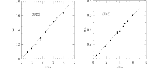
Figure 4: Maximal positive Lyapunov exponent as a function of the scaling parameter $(g^{2}E_{p}a)$ for (a) SU(2), (b) SU(3) gauge theory.

What about the other Lyapunov exponents? Their calculation for large lattices is prohibitively expensive, as there are in total $6(n^{2}-1)N^{3}$ degrees of freedom for SU($n$) gauge theory on a $N^{3}$ lattice, but Gong $\sevenrm^{\hbox{\immediate{?}}}$ has evaluated the complete spectrum for SU(2) on lattices of size $N=1,2$, and 3. The result again is a surprise: when the Lyapunov exponents are scaled by the maximal one, and are plotted on the interval $[0,1]$, the spectra for $N=2$ and $N=3$ are indistinguishable, and there is only a small difference between $N=1$ and $N=2$ (see Figure 5).

Figure 5: Spectrum of Lyapunov exponents for SU(2) lattice gauge theory. The black dots are for a $1^{3}$, the dotted line is for a $2^{3}$, and the solid line is for a $3^{3}$ lattice. The $18N^{3}$ exponents are plotted on the fixed interval [0,1] to exhibit the scaling with $N$.

The Lyapunov spectrum for SU(2) shows three separate components: there are $(6N^{3}-1)$ positive and negative exponents each, and there are $(6N^{3}+2)$ exponents that converge to zero in the limit $t\to\infty$. Their vanishing reflects the existence of $(3N^{3}+1)$ conservation laws: Gauss’ law at every lattice point and the overall energy conservation. Since the density of points on the line over the fixed interval [0,1] grows as $N^{3}$, this implies that the sum over positive Lyapunov exponents increases like the volume of the lattice, yielding a constant KS-entropy density $\dot{\sigma}_{\rm KS}$ in the thermodynamic limit. Gong finds

$$\dot{S}_{\rm KS}=\sum_{i}\lambda_{i}\theta(\lambda_{i})=c_{2}\lambda_{1}N^{3},$$ (15)

which together with (14) and the lattice volume $V=(Na)^{3}$ yields

$$\dot{\sigma}_{\rm KS}={1\over V}\dot{S}_{\rm KS}={1\over 3}b_{2}c_{2}g^{2}\varepsilon,$$ (16)

where $\varepsilon=3E_{p}/a^{3}$ is the average energy density on the lattice. (Note that there are $3N^{3}$ plaquettes.) No one has yet calculated the complete Lyapunov spectrum for SU(3), but I expect a similar relationship as (15) to hold in that case, too. The coefficient $c_{2}$ is not completely independent of the scaling variable $g^{2}E_{p}a$, but has a value around 2. We will return below to the question how the physically relevant value of $g^{2}E_{p}a$ can be chosen.

Physics Perspectives: Thermalization Time, Gluon Damping Rate

The instability of all degrees of freedom of the nonabelian gauge field (in the classical limit) leads to a very rapid “thermalization” of the energy density on the lattice. This is illustrated in Figure 6 showing the distribution of magnetic energy on the lattice plaquettes .$\sevenrm^{\hbox{\immediate{?}}}$ The initial state was chosen according to a random (not thermal) distribution of lattice link variables with vanishing electric field everywhere. Within two lattice units ($t/a=2$) the energy has been equilibrated between electric and magnetic fields and, as the exponentially falling distribution shows, has assumed the form of a Gibbs distribution. The time scale for this “thermalization” is in good agreement from the time scale estimated from the inverse of the maximal Lyapunov exponent which is $h\approx 0.6$ in lattice units in SU(3) at this energy density.

Figure 6: Logarithmic plot of the evolution of the magnetic energy density distribution on the lattice for SU(3) gauge theory. The distribution appears “thermalized” (exponential) after a time $t\approx 2$.

The fact that the energy density thermalizes on a time scale much shorter than that required for the numerical determination of the Lyapunov exponents (typically $t/a=1000$) allows us to relate the Lyapunov exponents to quantities in the presence of a thermal environment. First, we can replace the average energy per plaquette $E_{p}$ in (13) by the “temperature” $T$, because $E_{p}={2\over 3}(n^{2}-1)T$ for the classical, equilibrated SU($n$) gauge field. This implies that

$$h\approx\cases{{1\over 3}g^{2}T\approx 0.33g^{2}T&for SU(2),\cr\vskip 6.0pt plus 2.0pt minus 2.0pt\cr{8\over 15}g^{2}T\approx 0.53g^{2}T&for SU(3).\cr}$$ (17)

We can use this result to obtain a model independent, nonperturbative estimate of the thermalization time solely due to gauge field dynamics in QCD. To compensate for the lack of “running” of the gauge coupling constant in the context of our classical gauge field calculation, we may use the one-loop result for $g(T)^{2}$ in (17) to evaluate $\tau_{h}=h^{-1}$, as shown in Figure 7. Clearly, this time is much smaller than 0.5 fm/c for all relevant temperatures, indicating a very rapid thermalization of the available energy. One should note that the Lyapunov exponents usually approach their asymptotic values from above, i.e. the dynamical instabilities are actually greater before the energy has been completely thermalized. This indicates that thermalization of field configurations far away from equilibrium may proceed even more rapidly.

Figure 7: “Thermalization” time scale in SU(3) gauge theory as defined by the inverse of the maximal Lyapunov exponent (17), using $g(T)^{2}=16\pi^{2}/[11\ln(\pi T/\Lambda)^{2}]$ with $\Lambda=200$ MeV.

It first appeared as a remarkable coincidence that the maximal Lyapunov exponents for SU(2) and SU(3) agree within numerical errors with the analytically calculated damping rate of a nonabelian plasmon at rest :$\sevenrm^{\hbox{\immediate{?}}}$

$$\Gamma=2\gamma(0)=6.635{n\over 24\pi}g^{2}T\approx\cases{0.35g^{2}T&for SU(2),\cr 0.53g^{2}T&for SU(3).\cr}$$ (18)

[The reason for the factor 2 is that the plasmon pole is usally parametrized as $\omega_{p}(k)=\omega^{*}(k)-i\gamma(k)$, so that the energy density of the soft plasmon mode falls off as exp ($-2\gamma(0)t$).] The observation that the Lyapunov exponent is numerically evaluated in the vicinity of a “thermalized” field configuration over time scales that are much longer than those of thermal fluctuations allows us to establish a connection between these two quantities. According to (4) the Lyapunov exponents are determined from the long time behavior of solutions of the linearized equation for the fluctuation $a_{\mu}(x,t)$ around an exact solution $A_{\mu}(x,t)$ of the Yang-Mills equations. In the continuum limit this equation reads:

$$\left(g_{\mu\nu}D(A)^{2}-D_{\mu}(A)D_{\nu}(A)\right)a^{\nu}(x,t)-2i[F_{\mu\nu},a^{\nu}(x,t)]=0$$ (19)

where $D_{\mu}(A)$ denotes the gauge covariant derivative and $[F_{\mu\nu},a^{\nu}]$ denotes the Lie algebra commutator. Equation (19) is the usual starting point for quantization in a background field, but we will not impose here the background gauge constraint $D_{\nu}a^{\nu}=0$. The initial value problem for (19) can be solved by means of the retarded propagator Schwinger function in the background field.

$$a_{\mu}(x,t)=\int d^{3}x^{\prime}\Delta_{\rm ret}^{\mu\nu}(x,t;x^{\prime},0|A)a_{\nu}(x^{\prime},0).$$ (20)

$\Delta_{\rm ret}^{\mu\nu}$ has the formal representation as difference between the causal and the anticausal propagator:

$$\Delta_{\rm ret}^{\mu\nu}(A)=i\theta(t)\left[D_{\rm F}^{\mu\nu}(A)-D_{\rm F}^{\mu\nu^{*}}(A)\right]$$ (21)

Now recall that the maximal Lyapunov exponent is obtained from the long time average of the growth rate of $a^{\nu}(x,t)$. Assuming ergodicity, we may therefore replace the long-time average of the propagators by the canonical, i.e. thermal, average:

$$\overline{\Delta}_{\rm ret}^{\mu\nu}=i\theta(t)\left[D_{{\rm F},T}^{\mu\nu}-D_{{\rm F},T}^{\mu\nu^{*}}\right]$$ (22)

where $D_{{\rm F},T}^{\mu\nu}$ denotes the exact finite temperature Feynman propagator of the gauge field. Note that the causal Feynman propagator describes damped fluctuations, the anti-causal propagator $D_{\rm F}^{\mu\nu}$ describes exponentially growing perturbations. The only remaining obstacle before establishing the equivalence of $h$ and $2\gamma(0)$ is that the thermal average in (22) should be calculated for a classical emsemble of gauge fields, whereas the usual perturbative approach to $D_{{\rm F},T}^{\mu\nu}$ is based on the quantum mechanical ensemble. However, this difference turns out to be irrelevant for the plasmon damping rate $\gamma(0)$, although it has a large effect on the effective plasmon mass $\omega^{*}(0)$. This is not entirely fortuitous, because the damping rate is given by tree diagrams, such as Compton scattering and bremsstrahlung, that have an exact low-energy classical limit .$\sevenrm^{\hbox{\immediate{?},\penalty 301\hskip 0.91003pt plus 0.91003pt minus 0.91003pt{?}}}$ We can therefore identify the maximal Lyapunov exponent with (twice) the damping rate of the most unstable mode in a thermal nonabelianplasma, which turns out to be a plasmon at rest .$\sevenrm^{\hbox{\immediate{?}}}$

Conclusions and Outlook

The short thermalization time scales of less than 1 fm/c found in our studies of the time evolution of classical nonabelian gauge fields show why Hagedorn was right thirty years ago with his assumption that final states in “soft” strong interaction physics are populated statistically. The reason for the success of these classical studies is that the dynamical instabilities in thermal gauge theories are of order $g^{2}T$, which is a classical inverse length or time scale that does not involve $\hbar$. It would be interesting to see whether other quantities of order $g^{2}T$, such as the thermal magnetic screening mass on the “spatial” string tension, can also be calculated in the framework of classical Yang-Mills theory. This immediately leads to the problem of deriving an effective quasi-classical theory for thermal Yang-Mills theories at the length scale $(g^{2}T)^{-1}$ that consistently incorporates quantum effects from shorter distances in the form of transport coefficients. Presumably such an effective theory will contain a gauge invariant mass term of order $gT$ (as in the Taylor-Wong action) and a Langevin noise term describing the fluctuations due to interactions with hard thermal modes.

Another interesting problem concerns the application of real-time evolution of gauge fields to processes far off equilibrium as they occur in the earliest stage of hadron-hadron or nucleus-nucleus interactions. We have recently studied the instability of the superposition of two counter-propagating plane waves, i.e. of a standing abelian plane wave, in SU(2) Yang-Mills theory .$\sevenrm^{\hbox{\immediate{?}}}$ Here one finds that the Lyapunov exponent is proportional to the amplitude of the wave, not to the energy as it is the case in random fields. Once the coherent wave is only slightly perturbed it decays rapidly, exciting modes of all wavelengths, and quickly generates a thermal energy spectrum (see Figure 8). The evolution of more realistic initial configurations, such as the interaction between nonabelian wave packets, is presently under investigation.

Figure 8: (a) Total electric energy for a SU(2) standing plane wave as function of time. The dotted curve shows the stability of an initially abelian wave, the solid line shows the instability in the presence of small nonabelian perturbations. In that case the wave eventually decays into a quasithermal frequency spectrum (b).

References

- [1] R. Hagedorn, Suppl. Nuovo Cimento 3, 147 (1965).
- [2] J. J. M. Verbaarschot, H. A. Weidenmüller, and M. R. Zirnbauer, Phys. Rep. 129, 367 (1985); see also: C. Mahaux and H. A. Weidenmüller, Ann. Rev. Nucl. Part. Science 29, 1 (1979).
- [3] G. E. Mitchell, E. G. Bilpuch, P. M. Endt, J. F. Shriner, and T. von Egidy, Nucl. Instr. Meth. B46/47, 446 (1991).
- [4] see e.g. A. J. Lichtenberg and M. A. Liebermann, Regular and Stochastic Motion, (Springer-Verlag, New York, 1983).
- [5] S. G. Matinyan, G. K. Savvidy, and N. G. Ter-Arutyunyan-Savvidy, Zh. Eksp. Teor. Fiz. 80, 830 (1981) [Sov. Phys. JETP 53, 421 (1981)].
- [6] P. Dahlquist and G. Russberg, Phys. Rev. Lett. 65, 2837 (1990).
- [7] E. Haller, M. Köppel, and L. Cederbaum, Phys. Rev. Lett. 52, 1665 (1984).
- [8] B. Müller and A. Trayanov, Phys. Rev. Lett. 68, 3387 (1992).
- [9] T. S. Biró, C. Gong, B. Müller, and A. Trayanov, Int. J. Mod. Phys. C5, 113 (1994).
- [10] C. Gong, Phys. Lett. B298, 257 (1993).
- [11] C. Gong, Phys. Rev. D49, 2642 (1994).
- [12] C. Gong, Dissertation, Duke University, 1994 (unpublished).
- [13] E. Braaten and R. D. Pisarski, Phys. Rev. D42, 2156 (1990).
- [14] T. S. Biró, C. Gong, and B. Müller, to be published.
- [15] C. Gong, S. G. Matinyan, B. Müller, and A. Trayanov, Phys. Rev. D49, R607 (1994).