The three-loop free energy for pure gauge QCD

Abstract

We compute the free energy density for pure non-Abelian gauge theory at high temperature and zero chemical potential. The three-loop result to $O(g^{4})$ is

$$F = d_{\rm A}T^{4}{\pi^{2}\over 9}\Biggr{\{}{-}{1\over 5}{+}\left({g_{\rm A}\over 4\pi}\right)^{2}{-}{16\over\sqrt{3}}\left({g_{\rm A}\over 4\pi}\right)^{3}{-}48\left({g_{\rm A}\over 4\pi}\right)^{4}\ln\left(g_{\rm A}\over 2\pi\sqrt{3}\right)$$ (2)

$$\qquad{+}\left({g_{\rm A}\over 4\pi}\right)^{4}\Biggr{[}{22\over 3}\ln{\bar{\mu}\over 4\pi T}{+}{38\over 3}{\zeta^{\prime}(-3)\over\zeta(-3)}{-}{148\over 3}{\zeta^{\prime}(-1)\over\zeta(-1)}{-}4{\gamma_{\rm\scriptscriptstyle E}}{+}{64\over 5}\Biggr{]}{+}O(g_{\rm A}^{5})\Biggr{\}}\,,$$

where $T$ is the temperature, $\zeta$ is the Riemann zeta function, $g_{A}\equiv g(\bar{\mu})C_{\rm A}^{1/2}$, $\bar{\mu}$ is the $\overline{\rm MS}$ renormalization scale, $g(\bar{\mu})$ is the corresponding coupling constant, and $d_{\rm A}$ and $C_{\rm A}$ are the dimension and Casimir of the adjoint representation. We examine the sensitivity of this result to the choice of renormalization scale $\bar{\mu}$. We also give a result for the free energy of scalar $\phi^{4}$ theory, correcting a result previously given in the literature.

July 1994

I Introduction

The perturbative expansion of the free energy of hot non-Abelian gauge theory is of the form

$$F\sim T^{4}[c_{0}+c_{2}g^{2}+c_{3}g^{3}+(c^{\prime}_{4}\ln g+c_{4})g^{4}+O(g^{5})]\,,$$ (3)

where the $c_{i}$ are numerical coefficients (with some dependence on the choice of renormalization scale). The leading term is just the free energy of an ideal, ultrarelativistic gas of bosons. The first effect of interactions appears at $O(g^{2})$ and can be computed from two-loop diagrams such as fig. 1. To compute to higher order requires reorganizing perturbation theory to account for Debye screening of electric fields in the plasma and yields terms non-analytic in $g^{2}$ such as $O(g^{3})$ and $O(g^{4}\ln g)$. The full $O(g^{4})$ term requires a 3-loop calculation, and a full accounting of Debye screening at 3 loops would produce the $O(g^{5})$ terms. And that’s it; perturbation theory is believed incapable of pushing the calculation to any higher order. Beginning with four loops, infrared problems associated with magnetic confinement appear and non-perturbative $O(g^{6})$ contribution to the free energy. A complete three-loop calculation of the free energy therefore has the special significance that it’s the best anyone will ever do with perturbation theory. In this paper, our goal is slightly more modest. We shall only tackle the $O(g^{4})$ contribution from three loops and leave the $O(g^{5})$ contribution for another day.

FIG. 1.: A 2-loop contribution to the free energy.

Another interest of the three-loop calculation is that $O(g^{4})$ is the first order that begins to implement the renormalization-scale independence of the free energy. The coupling in (3) is really $g(\mu)$ where $\mu$ is some renormalization scale, and some of the coefficients depend on $\ln\mu$. The leading term that depends on the interaction is order $g^{2}(\mu)$, and by itself depends logarithmically on our choice of $\mu$. A change in this term due to a small change in renormalization scale,

$$g^{2}(\mu^{\prime})=g^{2}(\mu)+\beta_{0}g^{4}(\mu)\ln{\mu^{\prime 2}\over\mu^{2}}+\cdots\,,$$ (4)

is compensated by changes in higher-order contributions, first starting at $O(g^{4})$. The $O(g^{4})$ result should therefore have a flatter dependence on $\mu$ than the $O(g^{2})$ result. By checking this claim, we can get some idea of the theoretical uncertainties of lower-order calculations and perhaps learn some qualitative lessons that will carry over to other thermal quantities.

The $O(g^{3})$ piece of the free energy of non-Abelian gauge theory was previously obtained by Kapusta [3], and the $O(g^{4}\ln g)$ piece by Toimela [4]. We shall compute an analytic result for the full $O(g^{4})$ contribution. In somewhat related work, Corianò and Parwani [5] have recently studied high-temperature QED and numerically extracted the $O(g^{4})$ contribution, and Parwani [6] has also found the $O(g^{5})$ piece. (Unlike in non-Abelian gauge theory, the perturbation series in QED does not break down after $g^{5}$.) We shall only study pure gauge theory in this paper and do not include any fermions. Fermions will be included in a later work.

In the next section, we warm up to our task by computing the $O(g^{4})$ contribution to the free energy in pure scalar theory. The result for the basic, three-loop scalar diagram will be essential to the later gauge theory calculation, and we shall step through our technique for evaluating it analytically. We shall also briefly review the reorganization of the perturbation theory to account for the scalar analog of the Debye mass. In section III, we turn to non-abelian gauge theory and show how many 3-loop diagrams can be reduced to the scalar case. We then discuss how to evaluate the exceptions, which are two-particle-reducible diagrams. Finally, in section IV we discuss our results and examine the renormalization scale dependence. The details of several calculations needed along the way are relegated to appendices.

Throughout this paper we shall find it convenient to work almost exclusively in the Euclidean (imaginary time) formulation of thermal field theory. We shall conventionally refer to four-momenta with capital letters $K$ and to their components with lower-case letters: $K=(k_{0},\vec{k})$. Unless explicitly noted otherwise, all four-momenta are Euclidean with discrete frequencies $k_{0}=2\pi nT$.

II Scalar Theory

A Basics

Consider the theory of a real-scalar field with Euclidean Lagrangian

$${\cal L}_{\rm E}={1\over 2}(\partial\phi)^{2}+{1\over 4!}g^{2}\phi^{4}\,,$$ (5)

where we consider temperatures large enough that any zero-temperature mass can be neglected. The $O(g^{4})$ contribution to the free energy of this theory has been computed numerically by Frenkel, Saa, and Taylor [7]. In this section, we show how to obtain the result analytically and also correct an error in the derivation of Frenkel et al.

FIG. 2.: 1-loop contribution to the scalar thermal mass.

At high temperature, the scalar picks up a thermal contribution ${1\over 24}g^{2}T^{2}$ to its effective mass from the one-loop diagram of fig. 2. It is inefficient to do perturbation theory with zero-temperature scalar propagators, which do not account for this effect. We follow refs. [7, 8] and rewrite the Lagrangian as

$${\cal L}_{\rm E} = {\cal L}_{0}+{1\over 4!}g^{2}\phi^{4}-{1\over 48}g^{2}T^{2}\phi^{2}\,,$$ (6)

$${\cal L}_{0} = {1\over 2}\left[(\partial\phi)^{2}+{1\over 24}g^{2}T^{2}\phi^{2}\right]\,,$$ (7)

where the thermal mass has simply been added in and subtracted out so that nothing is changed. Now treat ${\cal L}_{0}$ as the unperturbed Lagrangian and the last term as a perturbation. This reorganization of the perturbative expansion is necessary to get a well-behaved expansion in $g$. One can imagine including yet-higher order corrections to the thermal mass in ${\cal L}_{0}$ above, but this is unnecessary and we shall not do so.

We regularize the theory by working in $d=4-2\epsilon$ dimensions with the modified minimal subtraction ($\overline{\rm MS}$) scheme. This corresponds to doing minimal subtraction (MS) and then changing the MS scale $\mu$ to the $\overline{\rm MS}$ scale $\bar{\mu}$ by the substitution

$$\mu^{2}={e^{{\gamma_{\rm\scriptscriptstyle E}}}\bar{\mu}^{2}\over 4\pi}\,.$$ (8)

In dimensional regularization, the one-loop thermal mass generated by fig. 2 is

$$m^{2}={1\over 2}g^{2}\hbox{$\sum$}\!\!\!\!\!\!\int_{P}{1\over P^{2}}\,,$$ (9)

where the integral-summation sign above is shorthand for the Euclidean integration

$$\hbox{$\sum$}\!\!\!\!\!\!\int_{P}\to\mu^{2\epsilon}T\sum_{p_{0}}\int{d^{3-2\epsilon}p\over(2\pi)^{3-2\epsilon}}$$ (10)

and the sum is over $p_{0}=2\pi nT$ for all integers $n$. Our reorganized Lagrangian is

$${\cal L}_{\rm E} = {\cal L}_{0}+{1\over 2}(Z_{1}-1)(\partial\phi)^{2}+{1\over 4!}\mu^{2\epsilon}Z_{2}g^{2}\phi^{4}-{1\over 2}m^{2}\phi^{2}\,,$$ (11)

$${\cal L}_{0} = {1\over 2}\left[(\partial\phi)^{2}+m^{2}\phi^{2}\right]\,,$$ (12)

where $Z_{1}$ and $Z_{2}$ are the usual zero-temperature multiplicative renormalizations:

$$Z_{1} = 1+O(g^{4})\,,$$ (13)

$$Z_{2} = 1+{3\over 2\epsilon}{g^{2}\over(4\pi)^{2}}+O(g^{4})\,.$$ (14)

FIG. 3.: Diagrams contributing to the free energy in scalar $\phi^{4}$ theory. Dots represent zero-temperature counter-terms, and crosses represent the “thermal counter-term” arising from the last term of (11).

The diagrams contributing to the free energy $F$ through three loops are shown in fig. 3, where all propagators represent the reorganized propagators of ${\cal L}_{0}$. The sum of these diagrams give $-F$. All of the diagrams except the last, the basketball diagram, are simple because they factorize into one-loop integrals. Diagrams (e-g) are particularly simple because they cancel each other at $O(g^{4})$. Diagram (a) represents the contribution to $-F$ of a non-interacting gas of bosons of mass $m$, and its high-temperature expansion is well-known [10]:

$$-{1\over 2}\hbox{$\sum$}\!\!\!\!\!\!\int_{P}\ln(P^{2}+m^{2})={\pi^{2}\over 90}T^{4}-{1\over 24}m^{2}T^{2} +{1\over 12\pi}m^{3}T+{1\over 64\pi^{2}}\left[{1\over\epsilon}+2\ln{\bar{\mu}\over 4\pi T}+2{\gamma_{\rm\scriptscriptstyle E}}\right]m^{4}$$ (16)

$$+O(m^{6}/T^{2},\epsilon)\,.$$

The one-loop integral needed for the remaining diagrams is obtained by differentiation with respect to $m^{2}$:

$$\hbox{$\sum$}\!\!\!\!\!\!\int_{P}{1\over P^{2}+m^{2}}={1\over 12}(1+\epsilon\iota_{\epsilon})T^{2} -{1\over 4\pi}mT-{1\over(4\pi)^{2}}m^{2}\left[{1\over\epsilon}+2\ln{\bar{\mu}\over 4\pi T}+2{\gamma_{\rm\scriptscriptstyle E}}\right]$$ (17)

$$+O(m^{4}/T^{2},\epsilon mT,\epsilon^{2}T^{2})\,.$$ (18)

We have shown only those terms that can contribute to the free energy at $O(g^{4})$, but this requires introducing a term of $O(\epsilon)$ that wasn’t needed in (16). The coefficient $\iota_{\epsilon}$ of this term is less well known, and it is worth taking a moment to focus on the $m=0$ case and review its simple derivation:

$$\hbox{$\sum$}\!\!\!\!\!\!\int_{P}{1\over P^{2}} = \mu^{2\epsilon}\int{d^{3-2\epsilon}p\over(2\pi)^{3-2\epsilon}}{1\over p^{2}}+2\mu^{2\epsilon}T\sum_{n=1}^{\infty}\int{d^{3-2\epsilon}p\over(2\pi)^{3-2\epsilon}}{1\over(2\pi nT)^{2}+p^{2}}$$ (19)

$$= 2\mu^{2\epsilon}T\int{d^{3-2\epsilon}p\over(2\pi)^{3-2\epsilon}}{1\over(2\pi T)^{2}+p^{2}}\sum_{n=1}^{\infty}n^{1-2\epsilon}$$ (20)

$$= {T^{2}\over 2\sqrt{\pi}}\left(\mu^{2}\over\pi T^{2}\right)^{\epsilon}\Gamma\left(-{\textstyle{1\over 2}}+\epsilon\right)\zeta(-1+2\epsilon)$$ (21)

$$= {T^{2}\over 12}\left[1+\epsilon\left(2\ln{\bar{\mu}\over 4\pi T}+2{\zeta^{\prime}(-1)\over\zeta(-1)}+2\right)\right]+O(\epsilon^{2})\,,$$ (22)

so that

$$\iota_{\epsilon}=2\ln{\bar{\mu}\over 4\pi T}+2{\zeta^{\prime}(-1)\over\zeta(-1)}+2\,.$$ (23)

With these tools, all of the diagrams but the last are straightforward. The individual contributions of each diagram are summarized in appendix A. Frenkel et al. [7] did not properly account for the $\iota_{\epsilon}$ term of (18) when evaluating diagrams (a–c).

B The basketball diagram

The last diagram of fig. 3 is more difficult. One simplification occurs because the diagram remains infrared convergent when the mass $m$ in the propagators is set to zero. This means that the presence of $m$ has only a sub-leading effect on the diagram, since $m$ itself is $O(g)$. We can ignore $m$ here if we are interested in the free energy only to $O(g^{4})$, and the basketball diagram is then proportional to

$$I_{\rm ball}\equiv\hbox{$\sum$}\!\!\!\!\!\!\int_{PQK}{1\over P^{2}Q^{2}K^{2}(P+Q+K)^{2}}\,.$$ (24)

Our attack on this integral starts with the observation that the basketball diagram of fig. 3(h) requires three independent four-momentum integrations if evaluated in momentum space but only one four-space integration if instead evaluated in configuration space. This suggests the diagram may be more tractable in configuration space. Indeed it would be if the diagram were ultraviolet (UV) convergent and we could set $\epsilon$ to zero. The configuration space propagator in four dimensions, with period $1/T$ in Euclidean time, is the relatively simple function

$$\Delta(\tau,\vec{r})={T\over 4\pi r}\,{\sinh(2\pi rT)\over[\cosh(2\pi rT)-\cos(2\pi\tau T)]}\,,$$ (25)

but in $4{-}2\epsilon$ dimensions it is a nightmare. We therefore need to first subtract out the UV divergent pieces, and evaluate them separately, so that we can then evaluate the remainder in four dimensions. We found, however, that making these subtractions is more convenient in momentum space than in configuration space. As a result, our derivation mixes the use of momentum and configuration space. First, we shall always treat the Euclidean time direction in frequency space. In configuration space for the remaining, spatial dimensions, the propagator $1/P^{2}$ then has a very simple form in exactly four dimensions:

$$\Delta(p_{0},\vec{r})={e^{-|p_{0}|r}\over 4\pi r}\,.$$ (26)

Our approach will be to start with the the momentum space form (24) of the basketball integral, convert it step by step into a configuration space form, and make needed subtractions as we go along.

1 A careless derivation

To simplify the presentation, let’s first forget about the UV subtractions and run through the derivation pretending that it makes sense in exactly four dimensions despite the UV divergences. We’ll later step through it a second time, handling the divergences more carefully. We start by noting that, by a shift of variables, the momentum integral (24) can be written in the form

$$I_{\rm ball}=\hbox{$\sum$}\!\!\!\!\!\!\int_{P}[\Pi(P)]^{2}\,,$$ (27)

where

$$\Pi(P)\equiv\hbox{$\sum$}\!\!\!\!\!\!\int_{Q}{1\over Q^{2}(P+Q)^{2}}\,.$$ (28)

Now let’s evaluate $\Pi(P)$ using configuration space and (26):

$$\Pi(P) = T\sum_{q_{0}}\int d^{3}r\,e^{i\vec{p}\cdot\vec{r}}\Delta(q_{0},\vec{r})\,\Delta(p_{0}+q_{0},\vec{r})$$ (29)

$$= {T\over(4\pi)^{2}}\sum_{q_{0}}\int d^{3}r\,{1\over r^{2}}e^{i\vec{p}\cdot\vec{r}}e^{-|q_{0}|r}e^{-|p_{0}+q_{0}|r}$$ (30)

$$= {T\over(4\pi)^{2}}\int d^{3}r\,{1\over r^{2}}e^{i\vec{p}\cdot\vec{r}}(\coth\bar{r}+|\bar{p}_{0}|)e^{-|p_{0}|r}\,,$$ (31)

where we have introduced the dimensionless variables

$$\bar{r}\equiv 2\pi Tr\,,\qquad\bar{p}_{0}\equiv p_{0}/2\pi T\,.$$ (32)

Plugging this into (27), the $\vec{p}$ integral becomes trivial, producing

$$I_{\rm ball} = {T^{3}\over(4\pi)^{4}}\sum_{p_{0}}\int d^{3}r\,r^{-4}(\coth\bar{r}+|\bar{p}_{0}|)^{2}e^{-2|p_{0}|r}$$ (33)

$$= {T^{4}\over 32\pi^{2}}\int\nolimits_{0}^{\infty}d\bar{r}\,\bar{r}^{-2}\left(\coth^{2}\bar{r}-\coth\bar{r}\,\,\partial_{\bar{r}}+\textstyle{1\over 4}\partial^{2}_{\bar{r}}\right)\coth\bar{r}\,.$$ (34)

As we shall discuss later, integrals like this can be performed analytically when they are convergent. The present result doesn’t make any sense, however, because the UV behavior ($\bar{r}\to 0$) of the integrand makes the integral divergent. We shall now repeat the above derivation while making necessary subtractions as we go along.

2 Subtraction of UV divergences

Let’s start with the expression (31) for $\Pi(P)$. This integral is logarithmically divergent in the ultraviolet. As usual with one-loop integrals at finite temperature, however, it can be made finite simply by subtracting out the zero-temperature contribution. So we write

$$\Pi(P)=\Pi^{(0)}(P)+\Pi^{(T)}(P)\,,$$ (35)

where $\Pi^{(0)}(P)$ is the zero-temperature result

$$\Pi^{(0)}(P)=\mu^{2\epsilon}\int{d^{d}Q\over(2\pi)^{d}}{1\over Q^{2}(P+Q)^{2}}={1\over(4\pi)^{2}}\left(4\pi\mu^{2}\over P^{2}\right)^{\epsilon}\left({1\over\epsilon}+2-{\gamma_{\rm\scriptscriptstyle E}}+O(\epsilon)\right)\,.$$ (36)

In four dimensions, $\Pi^{(T)}(P)$ can be obtained from (31) by subtracting out its $T\to 0$ limit (with $P$ fixed):

$$\Pi^{(T)}(P)={T\over(4\pi)^{2}}\int d^{3}r\,{1\over r^{2}}e^{i\vec{p}\cdot\vec{r}}\left(\coth\bar{r}-{1\over\bar{r}}\right)e^{-|p_{0}|r}+O(\epsilon)\,.$$ (37)

We now split our computation of the basketball diagram into

$$I_{\rm ball}=\hbox{$\sum$}\!\!\!\!\!\!\int[\Pi^{(T)}]^{2}+2\hbox{$\sum$}\!\!\!\!\!\!\int\Pi^{(T)}\Pi^{(0)}+\hbox{$\sum$}\!\!\!\!\!\!\int[\Pi^{(0)}]^{2}\,.$$ (38)

Though $\Pi^{(T)}$ is finite in four dimensions, the first term above is not because $\Pi^{(T)}\sim 1/P^{2}$ as $P{\to}\infty$; the first term therefore has a logarithmic UV divergence. The large $P$ (i.e. $P\gg T$) behavior of $\Pi^{(T)}$ is easy to extract by staring at the definition (28) of $\Pi$. The dominant contribution comes from routing the large momentum $P$ solely through one of the two propagators and then integrating over the relatively small momentum $Q\lesssim T$ in the other propagator:

$$\Pi^{(T)}(P)\to{2\over P^{2}}\left(\hbox{$\sum$}\!\!\!\!\!\!\int{1\over Q^{2}}\right)^{(T)}={2\over P^{2}}\hbox{$\sum$}\!\!\!\!\!\!\int{1\over Q^{2}}\,.$$ (39)

A more rigorous derivation may be found in appendix B. This limit is not restricted to four dimensions, so we are now in a position to subtract out the UV divergence in our integral:

$$\hbox{$\sum$}\!\!\!\!\!\!\int^{\prime}[\Pi^{(T)}]^{2}=\hbox{$\sum$}\!\!\!\!\!\!\int^{\prime}_{P}\Biggl{\{}[\Pi^{(T)}(P)]^{2}-\left({2\over P^{2}}\hbox{$\sum$}\!\!\!\!\!\!\int_{Q}{1\over Q^{2}}\right)^{2}\Biggr{\}}+\hbox{$\sum$}\!\!\!\!\!\!\int^{\prime}_{P}\left({2\over P^{2}}\hbox{$\sum$}\!\!\!\!\!\!\int_{Q}{1\over Q^{2}}\right)^{2}\,.$$ (40)

The first integral is now UV finite, and so we might hope to evaluate it in exactly four dimensions. However, it is not also infrared finite if we evaluate the $p_{0}=0$ term of the frequency sum; for $p_{0}=0$, the subtraction we made diverges linearly with $\vec{p}$ in the infrared. We shall therefore treat the $p_{0}=0$ mode separately and put primes on integrals, as we have above, to denote that this mode is excluded:

$$\hbox{$\sum$}\!\!\!\!\!\!\int^{\prime}_{P}\to\mu^{2\epsilon}T\sum_{p_{0}\not=0}\int{d^{3-2\epsilon}p\over(2\pi)^{3-2\epsilon}}\,.$$ (41)

We can now evaluate the first term of (40) in exactly four dimensions.

The leading large $P$ behavior (39) of $\Pi^{(T)}$ is related to the leading small $r$ behavior of the integrand in (37) and is given by

$$\Pi^{(T)}(P)\to{T\over(4\pi)^{2}}\int d^{3}r\,{1\over r^{2}}\,e^{i\vec{p}\cdot\vec{r}}\,\,{\bar{r}\over 3}\,\,e^{-|p_{0}|r}+O(\epsilon)\,.$$ (42)

Following the same steps as in the careless derivation of the previous section, we then obtain

$$\hbox{$\sum$}\!\!\!\!\!\!\int^{\prime}_{P} \left\{[\Pi^{(T)}(P)]^{2}-\left({2\over P^{2}}\hbox{$\sum$}\!\!\!\!\!\!\int_{Q}{1\over Q^{2}}\right)^{2}\right\}$$ (45)

$$\qquad\qquad={T^{3}\over(4\pi)^{4}}\sum_{p_{0}\not=0}\int d^{3}r\,r^{-4}\left[\left(\coth\bar{r}-{1\over\bar{r}}\right)^{2}-\left(\bar{r}\over 3\right)^{2}\right]e^{-2|p_{0}|r}+O(\epsilon)$$

$$\qquad\qquad={T^{4}\over 32\pi^{2}}\int\nolimits_{0}^{\infty}d\bar{r}\,\bar{r}^{-2}\left[\left(\coth\bar{r}-{1\over\bar{r}}\right)^{2}-\left(\bar{r}\over 3\right)^{2}\right](\coth\bar{r}-1)+O(\epsilon)\,.$$

This integral is both IR and UV convergent and can be evaluated using the techniques of appendix C to give

$$\hbox{$\sum$}\!\!\!\!\!\!\int^{\prime}_{P} \left\{[\Pi^{(T)}(P)]^{2}-\left({2\over P^{2}}\hbox{$\sum$}\!\!\!\!\!\!\int_{Q}{1\over Q^{2}}\right)^{2}\right\}$$ (47)

$$\qquad={1\over(4\pi)^{2}}\left(T^{2}\over 12\right)^{2}\left[-16{\zeta^{\prime}(-3)\over\zeta(-3)}+1152\zeta^{\prime}(-2)+24{\zeta^{\prime}(-1)\over\zeta(-1)}-8{\gamma_{\rm\scriptscriptstyle E}}+{28\over 15}\right]+O(\epsilon)\,.$$

The last term in (40) is easily evaluated in $4{-}2\epsilon$ dimensions using (22) and

$$\hbox{$\sum$}\!\!\!\!\!\!\int_{P}{1\over P^{4}}={1\over(4\pi)^{2}}\left[{1\over\epsilon}+2\ln{\bar{\mu}\over 4\pi T}+2{\gamma_{\rm\scriptscriptstyle E}}\right]+O(\epsilon)\,,$$ (48)

which may be obtained in a manner similar to (22).

Completing the derivation of the $[\Pi^{(T)}]^{2}$ contribution to $I_{\rm ball}$ now just requires adding in the contribution of the $p_{0}=0$ mode, which is UV convergent and does not require any subtractions:

$$T\int{d^{d-1}p\over(2\pi)^{d-1}}[\Pi^{(T)}(0,p)]^{2} = {T^{4}\over 32\pi^{2}}\int\nolimits_{0}^{\infty}d\bar{r}\,\bar{r}^{-2}\left(\coth\bar{r}-{1\over\bar{r}}\right)^{2}+O(\epsilon)$$ (49)

$$= {1\over(4\pi)^{2}}\left(T^{2}\over 12\right)^{2}\left[-1152\zeta^{\prime}(-2)\right]+O(\epsilon)\,,$$ (50)

where we have again used the techniques of appendix C to do the integral. Putting together (22, 40, 47, 48, 50) then gives

$$\hbox{$\sum$}\!\!\!\!\!\!\int[\Pi^{(T)}]^{2}={1\over(4\pi)^{2}}\left(T^{2}\over 12\right)^{2}\left[{4\over\epsilon}+24\ln{\bar{\mu}\over 4\pi T}-16{\zeta^{\prime}(-3)\over\zeta(-3)}+40{\zeta^{\prime}(-1)\over\zeta(-1)}+{268\over 15}\right]+O(\epsilon)\,.$$ (51)

Now that we’ve covered the basic ideas of our technique, we’ll leave the evaluation of the remaining two terms in (38) to appendix D. The final result for the basketball integral (24) is

$$I_{\rm ball}={1\over(4\pi)^{2}}\left(T^{2}\over 12\right)^{2}\left[{6\over\epsilon}+36\ln{\bar{\mu}\over 4\pi T}-12{\zeta^{\prime}(-3)\over\zeta(-3)}+48{\zeta^{\prime}(-1)\over\zeta(-1)}+{182\over 5}\right]+O(\epsilon)\,.$$ (52)

This agrees with the numerical result of ref. [7]. We should mention that our analytic result can also be obtained from the integrals generated by a real-time analysis, such as in ref. [7], and we show how to do this in appendix E. We have found it simpler to stick to Euclidean space, however, to evaluate diagrams involving double poles $1/P^{4}$ which will appear later in gauge theories.

C The result

Putting together all the diagrams, which are independently tabulated in appendix A, one finds that the free energy in $\phi^{4}$ theory at high temperature is

$$F = T^{4}{\pi^{2}\over 9}\Biggr{\{}{-}{1\over 10}{+}{1\over 8}\left(g\over 4\pi\right)^{2}{-}{1\over\sqrt{6}}\left(g\over 4\pi\right)^{3}$$ (54)

$$\qquad{+}\left(g\over 4\pi\right)^{4}\Biggr{[}{-}{3\over 8}\ln{\bar{\mu}\over 4\pi T}{+}{1\over 4}{\zeta^{\prime}(-3)\over\zeta(-3)}{-}{1\over 2}{\zeta^{\prime}(-1)\over\zeta(-1)}{-}{1\over 8}{\gamma_{\rm\scriptscriptstyle E}}{+}{59\over 120}\Biggr{]}{+}O(g^{5})\Biggr{\}}\,.$$

FIG. 4.: The setting sun diagram.

Before leaving scalar theory, we should mention one other basic scalar integral which appears in the literature [8, 9] and which will be needed when we analyze gauge theories. It is the integral corresponding to the setting sun diagram of fig. 4,

$$I_{\rm sun}(m_{1},m_{2},m_{3})\equiv\hbox{$\sum$}\!\!\!\!\!\!\int_{PQ}{1\over(P^{2}+m_{1}^{2})(Q^{2}+m_{2}^{2})[(P+Q)^{2}+m_{3}^{2}]}\,,$$ (55)

evaluated to leading order in the masses. It has previously only been evaluated numerically [8], but the same techniques we applied to the basketball diagram can be used to obtain an analytic result. We give the derivation in appendix F, with the result that

$$I_{\rm sun}={T^{2}\over(4\pi)^{2}}\left[{1\over 4\epsilon}+\ln\left(\bar{\mu}\over m_{1}+m_{2}+m_{3}\right)+{1\over 2}\right]+O(m,\epsilon)\,.$$ (56)

III Nonabelian gauge theory

We now turn to pure non-Abelian gauge theory, given by the Lagrangian

$${\cal L}_{\rm E}={1\over 4}\left(\partial_{\mu}A_{\nu}^{a}-\partial_{\nu}A_{\mu}^{a}+gf^{abc}A_{\mu}^{b}A_{\nu}^{c}\right)^{2}+(\hbox{gauge fixing})\,.$$ (57)

We shall work exclusively in Feynman gauge. (It would be nice to explicitly verify that our results are independent of gauge choice, but we have not done so.) Let $d_{\rm A}$ and $C_{\rm A}$ be the dimension and Casimir of the adjoint representation, with $C_{\rm A}$ given by

$$f^{abc}f^{dbc}=C_{\rm A}\delta^{ad}\,.$$ (58)

For SU($N$), they are

$$d_{\rm A}=N^{2}-1\,,\qquad\qquad\qquad C_{\rm A}=N\,.$$ (59)

It is also convenient to define the effective coupling $g_{\rm A}$ of the adjoint representation by

$$g_{\rm A}^{2}\equiv g^{2}C_{\rm A}\,.$$ (60)

As before, we shall regulate the theory with dimensional regularization in the $\overline{\rm MS}$ scheme.

FIG. 5.: The one-loop gluon self energy.

As in the scalar case, one-loop effects induce a thermal mass contribution. This mass is given by the one-loop self-energy $\Pi_{\mu\nu}$ at zero momentum, and in Euclidean space a mass is generated for $A_{0}$ but not for $\vec{A}$. This mass $M$ is the Debye screening mass for static electric fields and may be evaluated from the diagrams of fig. 5 as

$$M^{2}\delta^{ab}=\Pi^{ab}_{\mu\mu}(0)=g_{\rm A}^{2}(d-2)^{2}\hbox{$\sum$}\!\!\!\!\!\!\int_{Q}{1\over Q^{2}}\delta^{ab}\,.$$ (61)

In four dimensions, $M^{2}$ is simply $g_{\rm A}^{2}T^{2}/3$. In the gauge theory calculation, we find it calculationally convenient to use a slightly different reorganization of perturbation theory than we did for in the scalar case. The success of the reorganization only depends on the behavior of the propagator in the infrared ($p_{0}{=}0$, $p{\ll}T$), where the mass cannot be treated as a perturbation. We follow ref. [9] and only introduce the mass for the $p_{0}=0$ mode. That is, we rewrite our Lagrangian density, in frequency space, as

$${\cal L}_{\rm E}=\left({\cal L}_{\rm E}+{\textstyle{1\over 2}}M^{2}A^{a}_{0}A^{a}_{0}\delta_{p_{0}}\right)-{\textstyle{1\over 2}}M^{2}A^{a}_{0}A^{a}_{0}\delta_{p_{0}}\,,$$ (62)

where $\delta_{p_{0}}$ is shorthand for the the Kronecker delta function $\delta_{p_{0},0}$. Then we absorb the first $A_{0}^{2}$ term into our unperturbed Lagrangian ${\cal L}_{0}$ and treat the second $A_{0}^{2}$ term as a perturbation.

Since the necessity of resummation is an infrared phenomena, associated with the mass scale $gT$, it is worth noting that the prescription (62) can be naturally expressed in the language of decoupling. First imagine integrating out all the physics associated with scales $\gtrsim T$. In particular, integrating out all of the $p_{0}\not=0$ modes in Euclidean space generates an effective three dimensional theory of the remaining $p_{0}=0$ modes. This effective theory will have the thermal mass for $A_{0}$ and other interactions induced by the heavy modes, which can be computed to any desired order in perturbation theory. Only then does one finally integrate out the $p_{0}=0$ modes after deciding on a sensible partition of the effective three-dimensional Lagrangian into an unperturbed piece, containing the thermal mass terms, and a perturbative piece. Rather than carry out the reduction to this effective theory explicitly, however, we find it simplest to just introduce the reorganization (62). We refer the reader to sections III.D and VI of ref. [9] for details of how to implement this form of reorganization on two-loop graphs.

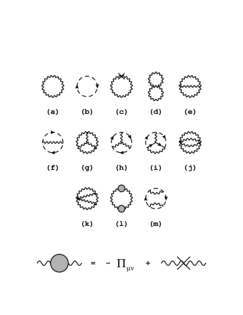
FIG. 6.: Diagrams contributing to the free energy in gauge theory. The crosses are the “thermal counter-terms” arising from the last term of (62). We have not explicitly shown any zero-temperature counter-terms, and each diagram should be multiplied by the appropriate multiplicative renormalizations for vertices and propagators.

The diagrams that contribute to the free energy are shown in fig. 6. The diagrams involving only one-loop integrations are trivial, and the resummation and the two-loop graphs can be handled by the methods of ref. [9]. Let’s therefore focus on the three-loop diagrams. The first potential problem is that some of the individual diagrams, such as fig. 7, are infrared divergent because of the masslessness of the $\vec{A}$ propagator. However, the particular combination we have shown in fig. 6(l) is well-behaved in the infrared since the shaded blobs,

$$\Delta\Pi_{\mu\nu}\equiv\Pi_{\mu\nu}(P)-\Pi_{\mu\nu}(0)\delta_{p_{0}}\,,$$ (63)

are $O(pT)$ for $(p_{0}{=}0,\vec{p}{\to}0)$. We can then also drop the Debye mass $M$ in evaluating the three-loop graphs since, as in the scalar case, the corrections to the free energy will be beyond $O(g^{4})$.

FIG. 7.: A diagram with infrared problems.

All of the three loop diagrams except (l) can be reduced to the scalar basketball integral of (24). For example, diagram (i) is equal to

$$-\mu^{2\epsilon}F^{\rm i}=-{1\over 8}d_{\rm A}g_{\rm A}^{2}\hbox{$\sum$}\!\!\!\!\!\!\int_{PQK}{P\cdot(Q-K)\,(P-K)\cdot Q\over P^{2}Q^{2}K^{2}(P-Q)^{2}(Q-K)^{2}(K-P)^{2}}\,.$$ (64)

This may be reduced by (1) expanding numerator factors in terms of denominator factors to cancel factors between numerator and denominator, such as

$$P\cdot(Q-K)={\textstyle{1\over 2}}[(K-P)^{2}-K^{2}-(P-Q)^{2}+Q^{2}]\,;$$ (65)

(2) performing appropriate changes of variables to collect similar terms; and (3) using the identity

$$\hbox{$\sum$}\!\!\!\!\!\!\int_{P}{P_{\mu}\over(P+Q)^{2}(P+K)^{2}}=-{Q_{\mu}+K_{\mu}\over 2}\hbox{$\sum$}\!\!\!\!\!\!\int_{P}{1\over(P+Q)^{2}(P+K)^{2}}\,,$$ (66)

which follows by averaging the left-hand side with itself, after applying the change of variables $P\to{-}P{-}Q{-}K$. Appendix G steps through this reduction for the example (64), and the reductions of diagrams (g–k,m) are all tabulated in appendix A.

Unfortunately, diagram (l) cannot be reduced to the scalar basketball. If one tries the above tricks, one finds a term of the form

$$I_{\rm hard}\equiv\hbox{$\sum$}\!\!\!\!\!\!\int_{PQK}{(Q\cdot K)^{2}\over P^{4}Q^{2}K^{2}(P+Q)^{2}(P+K)^{2}}$$ (67)

for which the tricks fail to remove the numerator factor. So we have a new basic integral that we must evaluate, like the basketball integral of scalar theory. We have found it more tractable, however, to apply our integration method directly to the original diagram (l) because the orthogonality of the one-loop self-energy $\Pi_{\mu\nu}(P)$ to $P_{\mu}$ leads to useful algebraic simplifications. Diagram (l) is proportional to

$$d_{\rm A}g_{\rm A}^{4}I_{\rm qcd}\equiv\hbox{$\sum$}\!\!\!\!\!\!\int_{P}{1\over P^{4}}{\rm tr}[\Delta\Pi_{\mu\nu}(P)]^{2}\,.$$ (68)

The evaluation of $I_{\rm qcd}$ is somewhat similar to that of the basketball integral $I_{\rm ball}$ and is presented in appendix H. We should mention, however, that the derivation is more complicated and involves a miraculous cancelation between two complicated integrals that we don’t know how to calculate individually. The appearance and cancelation of such complications suggests that we may still be missing the most elegant method for making these calculations.

All the results for individual graphs are collected in appendix A, with the final result that

$$F = d_{\rm A}T^{4}{\pi^{2}\over 9}\Biggr{\{}{-}{1\over 5}{+}\left({g_{\rm A}\over 4\pi}\right)^{2}{-}{16\over\sqrt{3}}\left({g_{\rm A}\over 4\pi}\right)^{3}{-}48\left({g_{\rm A}\over 4\pi}\right)^{4}\ln\left(g_{\rm A}\over 2\pi\sqrt{3}\right)$$ (70)

$$\qquad{+}\left({g_{\rm A}\over 4\pi}\right)^{4}\Biggr{[}{22\over 3}\ln{\bar{\mu}\over 4\pi T}{+}{38\over 3}{\zeta^{\prime}(-3)\over\zeta(-3)}{-}{148\over 3}{\zeta^{\prime}(-1)\over\zeta(-1)}{-}4{\gamma_{\rm\scriptscriptstyle E}}{+}{64\over 5}\Biggr{]}{+}O(g_{\rm A}^{5})\Biggr{\}}\,.$$

For those who prefer $\zeta$ functions with positive arguments,

$${\zeta^{\prime}(-n)\over\zeta(-n)}=\ln(2\pi)+{\gamma_{\rm\scriptscriptstyle E}}-\sum_{k=1}^{n}{1\over k}-{\zeta^{\prime}(1+n)\over\zeta(1+n)}\,,\qquad\hbox{$n$ odd}\,.$$ (71)

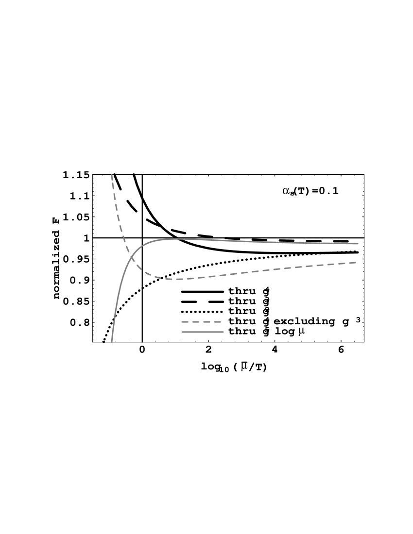
FIG. 8.: The dependence of the free energy $F$ on the choice of renormalization scale $\bar{\mu}$ for pure gauge QCD with $\alpha_{\rm s}(T)=0.1$. The free energy is normalized in units of the ideal gas result $-d_{\rm A}\pi^{2}T^{4}/45$. The thick solid, dashed, and dotted lines are the results for $F$ including terms through $g^{4}$, $g^{3}$, and $g^{2}$ respectively. The light solid curve is the $g^{4}$ result plus the $g^{5}\ln(\bar{\mu}/T)$ term required by renormalization group invariance. The light dashed curve is the $g^{4}$ result minus the $g^{3}$ term.

IV Discussion

Evaluated numerically, our result (70) is

$$F=-d_{\rm A}{\pi^{2}T^{4}\over 45} \biggl{[}1-0.31250\left(g_{\rm A}\over\pi\right)^{2}+0.72168\left(g_{\rm A}\over\pi\right)^{3}$$ (73)

$$\qquad+\left(g_{\rm A}\over\pi\right)^{4}\left(0.93750\ln{g_{\rm A}\over\pi}-0.14323\ln{\bar{\mu}\over T}+0.74582\right)+O(g_{\rm A}^{5})\biggr{]}\,.$$

We have chosen the expansion parameter $g_{\rm A}/\pi$ simply because it makes all the coefficients $O(1)$.

Now we can ask whether perturbation theory is behaving well for physically-realized values of the couplings. In particular, we can investigate (1) the size of corrections from different orders for a fixed choice of renormalization scale, such as $\bar{\mu}=T$, and (2) whether higher-order results are less sensitive to the choice of the renormalization scale $\bar{\mu}$ than lower-order results. This information is summarized in fig. 8 for pure gauge QCD with $\alpha_{\rm s}(T)=0.1$, which for real QCD would correspond to a temperature around the electroweak scale. We have used the two-loop renormalization group to compute $g(\mu)$:

$${1\over g_{\rm A}^{2}(\mu)}\approx{1\over g_{\rm A}^{2}(T)}-\beta_{0}\ln{\bar{\mu}\over T}+{\beta_{1}\over\beta_{0}}\ln\left(1-\beta_{0}g_{\rm A}^{2}(T)\ln{\bar{\mu}\over T}\right)\,,$$ (74)

where

$$\beta_{0}=-{22\over 3(4\pi)^{2}}\,,\qquad\beta_{1}=-{68\over 3(4\pi)^{4}}\,.$$ (75)

At $\bar{\mu}=T$, the terms of (73) for $\alpha_{\rm s}(T){=}0.1$ are

$$F=-d_{\rm A}{\pi^{2}T^{4}\over 45}[1-0.12+0.17+(-0.07+0+0.11)+O(g_{\rm A}^{5})]\,.$$ (76)

The behavior of the perturbative expansion doesn’t look particularly good, though a partial cancelation between the $g^{4}\ln g$ and $g^{4}$ terms makes the total $O(g^{4})$ contribution relatively small. Alternatively, examine the sensitivity of the result to the choice of renormalization scale by examining the slopes of the curves in fig. 8 at $\bar{\mu}=T$. Contrary to one’s expectation for a well-behaved perturbative expansion, the $O(g^{4})$ result is more sensitive to $\bar{\mu}$ than the $O(g^{2})$ or $O(g^{3})$ results.

FIG. 9.: The same as fig. 8 but for $\alpha_{\rm s}(T)=0.02$ [which is identical to SU(2) gauge theory with $\alpha_{\rm w}(T)\approx 1/33$].

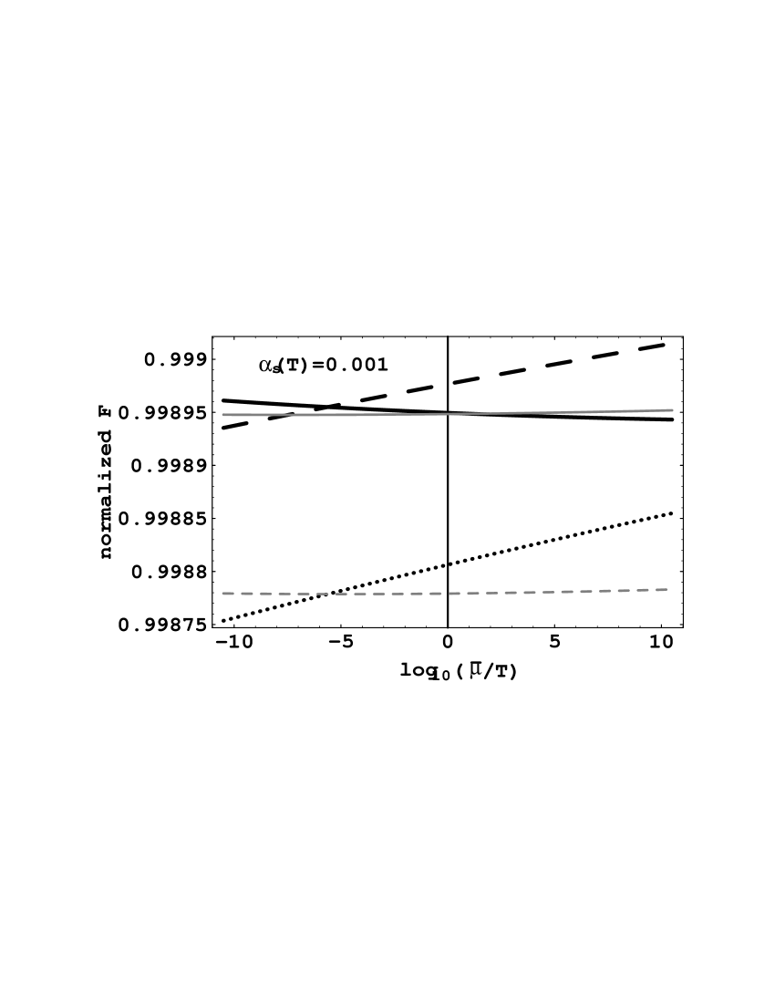
FIG. 10.: The same as fig. 8 but for $\alpha_{\rm s}(T)=0.001$.

The $O(g^{4})$ result has to be less sensitive to $\bar{\mu}$ if $g$ is sufficiently small. Fig. 9 shows the dependence for $\alpha_{\rm s}(T)=0.02$. This is equivalent to a system of interest—pure electroweak theory at the electroweak scale, with $\alpha_{\rm w}\approx 1/33$. Yet still the $O(g^{4})$ result is no less sensitive than the $O(g^{2})$ result. Fig. 10 shows $\alpha_{\rm s}(T)=0.001$, where we finally see the expected behavior. (In six-flavor QCD, this $\alpha_{\rm s}$ would correspond to a temperature of $10^{387}$ GeV.)

The source of the sensitivity problem can be found by remembering that the $g^{3}$ term probes different physics than the $g^{2}$ term: the $g^{2}$ term is produced by particles with hard thermal momenta of order $T$, while the $g^{3}$ term arises from the interactions of particles with softer momentum of order $gT$. Since the $g^{3}$ term is the leading-order contribution of the physics of scale $gT$, it perhaps should be treated independently of the $g^{2}$ term when discussing whether the perturbation expansion is well-behaved. The $g^{4}$ terms reduce the sensitivity of the $g^{2}$ term to $\bar{\mu}$, and the $g^{5}$ contribution will be needed to reduce the sensitivity of the $g^{3}$ term. The light dashed line in figs. 8–9 show the result of the free energy through $O(g^{4})$ if the $g^{3}$ term is artificially excluded. The sensitivity to $\bar{\mu}$, compared to the $O(g^{2})$ result, is indeed much better than before.

In order to put the $O(g^{3})$ term back in, we have tried adding the $g^{5}\ln\mu$ term that’s determined by renormalization group invariance. The light solid lines in figs. 8–9 represent our result (70) with the addition

$$\Delta F=d_{\rm A}T^{4}{\pi^{2}\over 9}\Biggr{\{}{-}{16\over\sqrt{3}}\left(g_{\rm A}\over 4\pi\right)^{5}\left[11\ln{\bar{\mu}\over 4\pi T}\right]\Biggl{\}}\,.$$ (77)

The results are much better behaved than the $O(g^{4})$ results discussed earlier. Of course, the constant under the log at $O(g^{5})$ is unknown and will change the curves somewhat. Our understanding of whether perturbative results are indeed well-behaved in high-temperature QCD, for realistic coupling constants, would therefore benefit by a true calculation to $O(g^{5})$—the last order accessible to perturbation theory.

This work was supported by the U.S. Department of Energy, grant DE-FG06-91ER40614. We thank Larry Yaffe, and most especially Lowell Brown, for their repeated suggestions that we try analyzing our basic diagrams in configuration space using the simple form of the propagators in three spatial dimensions. We also thank Rajesh Parwani and Claudio Corianò for useful discussions.

A Results for individual graphs

1 Scalar theory

The diagrams of fig. 3 are given by

$$-\mu^{2\epsilon}F^{\rm a}=-{1\over 2}\hbox{$\sum$}\!\!\!\!\!\!\int\ln(P^{2}+m^{2})\,,$$ (A2)

$$-\mu^{2\epsilon}F^{\rm b}=-{1\over 8}g^{2}\left(\hbox{$\sum$}\!\!\!\!\!\!\int{1\over P^{2}+m^{2}}\right)^{2}\,,$$ (A3)

$$-\mu^{2\epsilon}F^{\rm c}={1\over 2}m^{2}\hbox{$\sum$}\!\!\!\!\!\!\int{1\over P^{2}+m^{2}}\,,$$ (A4)

$$-\mu^{2\epsilon}F^{\rm d}=-{1\over 8}\left(3g^{4}\over 32\pi^{2}\epsilon\right)\left(\hbox{$\sum$}\!\!\!\!\!\!\int{1\over P^{2}+m^{2}}\right)^{2}+O(g^{6})\,,$$ (A5)

$$-\mu^{2\epsilon}(F^{\rm e}+F^{\rm f}+F^{\rm g})=O(g^{5})\,,$$ (A6)

$$-\mu^{2\epsilon}F^{\rm h}={1\over 48}g^{4}I_{\rm ball}+O(g^{5})\,.$$ (A7h)

2 Gauge theory

Writing $F=\mu^{-2\epsilon}d_{\rm A}{\cal F}$ and ignoring terms of $O(\epsilon)$, the diagrams of fig. 6 are given by

$$-{\cal F}^{\rm a} = -{d\over 2}\hbox{$\sum$}\!\!\!\!\!\!\int\ln P^{2}+{1\over 12\pi}M^{3}T\,,$$ (A9)

$$-{\cal F}^{\rm b} = \hbox{$\sum$}\!\!\!\!\!\!\int\ln P^{2}\,,$$ (A10)

$$-{\cal F}^{\rm c} = -{1\over 8\pi}(M_{1}^{2}+M_{2}^{2}+M_{3}^{2})MT\,,$$ (A11)

$$-{\cal F}^{\rm d} = -{1\over 4}g_{\rm A}^{2}Z_{g}^{2}d(d-1)\left(\hbox{$\sum$}\!\!\!\!\!\!\int{1\over P^{2}}\right)^{2}+{1\over 8\pi}M_{1}^{2}MT\,,$$ (A12)

$$-{\cal F}^{\rm e} = g_{\rm A}^{2}Z_{g}^{2}\left[{3\over 4}(d-1)\left(\hbox{$\sum$}\!\!\!\!\!\!\int{1\over P^{2}}\right)^{2}+\delta_{1}+\delta_{2}\right]\,,$$ (A15)

$$\delta_{1}=-M^{2}\hbox{$\sum$}\!\!\!\!\!\!\int{\delta_{p_{0}}(1-\delta_{q_{0}})\over(P^{2}+M^{2})Q^{2}(P+Q)^{2}}+\left(d-{3\over 2}\right)I_{\rm resum}+{1\over 8\pi}{M_{2}^{2}MT\over g_{\rm A}^{2}Z_{g}^{2}}\,,$$

$$\delta_{2}=-{1\over 4}{M^{2}T^{2}\over(4\pi)^{2}}-M^{2}\hbox{$\sum$}\!\!\!\!\!\!\int{\delta_{p_{0}}\delta_{q_{0}}\over(P^{2}+M^{2})(Q^{2}+M^{2})(P+Q)^{2}}\,,$$

$$-{\cal F}^{\rm f} = g_{\rm A}^{2}Z_{g}^{2}\left[-{1\over 4}\left(\hbox{$\sum$}\!\!\!\!\!\!\int{1\over P^{2}}\right)^{2}-{1\over 2}I_{\rm resum}\right]+{1\over 8\pi}M_{3}^{2}MT\,,$$ (A16)

$$-{\cal F}^{\rm g} = \left({5\over 8}d-{23\over 32}\right)g_{\rm A}^{4}I_{\rm ball}+O(g^{5})\,,$$ (A17)

$$-{\cal F}^{\rm h} = -{1\over 16}g_{\rm A}^{4}I_{\rm ball}+O(g^{5})\,,$$ (A18)

$$-{\cal F}^{\rm i} = -{1\over 32}g_{\rm A}^{4}I_{\rm ball}+O(g^{5})\,,$$ (A19)

$$-{\cal F}^{\rm j} = {3\over 16}d(d-1)g_{\rm A}^{4}I_{\rm ball}+O(g^{5})\,,$$ (A20)

$$-{\cal F}^{\rm k} = -{27\over 16}(d-1)g_{\rm A}^{4}I_{\rm ball}+O(g^{5})\,,$$ (A21)

$$-{\cal F}^{\rm l} = {1\over 4}g_{\rm A}^{4}I_{\rm qcd}+O(g^{5})\,,$$ (A22)

$$-{\cal F}^{\rm m} = -{1\over 8}g_{\rm A}^{4}I_{\rm ball}+O(g^{5})\,.$$ (A23)

The multiplicative renormalization constant used for the coupling is given by

$$g_{\rm bare}=Z_{g}g=\left[1-{11\over 6}{g_{\rm A}^{2}\over(4\pi)^{2}\epsilon}+O(g^{4})\right]g\,.$$ (A24)

Wave function renormalization constants are unnecessary because they cancel between vertices and propagators. [To this end, the most convenient choice of $M$ is

$$M^{2}=g_{\rm A}^{2}Z_{g}^{2}Z_{A}^{2}(d-2)^{2}\hbox{$\sum$}\!\!\!\!\!\!\int{1\over P^{2}}\,$$ (A25)

which differs from (61) by the introduction of $Z_{g}^{2}$ and the photon wave function renormalization $Z_{A}^{2}$. At $O(g^{4})$, however, this is not an issue—the factor of $Z_{g}^{2}Z_{A}^{2}$ in $M^{2}$ can be ignored for all of our diagrams.] $M_{1}^{2}$, $M_{2}^{2}$, and $M_{3}^{2}$ denote the three pieces of $M^{2}$ originating, respectively, from the three diagrams in fig. 5. We will not give explicit formulas for these pieces because they explicitly cancel between diagrams (c–f).

The integrals needed above are given by (16, 18, 52, A34, F5, F29, H40). The integral $I_{\rm resum}$ is defined by

$$I_{\rm resum} \equiv \hbox{$\sum$}\!\!\!\!\!\!\int\left[{\delta_{p_{0}}\over P^{2}+M^{2}}-{\delta_{p_{0}}\over P^{2}}\right]\left[{q_{0}^{2}\over Q^{2}(P+Q)^{2}}-{q_{0}^{2}\over Q^{4}}\right]$$ (A26)

$$= -\hbox{$\sum$}\!\!\!\!\!\!\int\delta_{p_{0}}{M^{2}\over P^{4}}\left[{q_{0}^{2}\over Q^{2}(P+Q)^{2}}-{q_{0}^{2}\over Q^{4}}\right]+O(g^{3})$$ (A27)

and will be discussed below.

The effect of the thermal mass term in the $p_{0}{=}0$ gauge propagator appears fairly simply in the last terms of (A 2a, d) and in (A 2c). The case of diagram (e) is a little more complicated. The first term of (A 2e) is the result when $M$ is ignored. $\delta_{1}$ is the correction to this result for the contribution to the diagram where exactly one of the three propagators has $p_{0}=0$, and $\delta_{2}$ is the correction for the contribution where all three have $p_{0}=0$. So, for instance,

$$\delta_{1}=\left\{{1\over 4}\hbox{$\sum$}\!\!\!\!\!\!\int{\delta_{p_{0}}(1-\delta_{q_{0}})\over(P^{2}+M^{2})Q^{2}(P+Q)^{2}}\right\}\left[(P-Q)_{\mu}\delta_{0\nu}+2Q_{0}\delta_{\mu\nu}-(2P+Q)_{\nu}\delta_{\mu 0}\right]^{2}-\{M{\to}0\}\,,$$ (A28)

where the factor in brackets is the triple gauge vertex. Using the reduction tricks described after (64), $\delta_{1}$ may be reduced to

$$\delta_{1}=-M^{2}\hbox{$\sum$}\!\!\!\!\!\!\int{\delta_{p_{0}}(1-\delta_{q_{0}})\over(P^{2}+M^{2})Q^{2}(P+Q)^{2}} + \left(d-{\textstyle{3\over 2}}\right)\hbox{$\sum$}\!\!\!\!\!\!\int\left[{\delta_{p_{0}}\over P^{2}+M^{2}}-{\delta_{p_{0}}\over P^{2}}\right]{q_{0}^{2}\over Q^{2}(P+Q)^{2}}$$ (A29)

$$+ {1\over 2}\hbox{$\sum$}\!\!\!\!\!\!\int{\delta_{p_{0}}\over(P^{2}+M^{2})}\,{1\over Q^{2}}\,,$$ (A30)

which may be recast in the form shown in (A 2e). $\delta_{2}$, and the mass effects in (A 2f), are calculated similarly.

$I_{\rm resum}$ is easily evaluated by taking the form (A27) and scaling all three-momenta by $|q_{0}|$:

$$I_{\rm resum}=-M^{2} T^{2}\mu^{4\epsilon}\sum_{q_{0}}|q_{0}|^{2d-8}$$ (A32)

$$\times\int{d^{d-1}p\over(2\pi)^{d-1}}{d^{d-1}q\over(2\pi)^{d-1}}{1\over p^{4}}\left[{1\over(1+q^{2})(1+|\vec{p}+\vec{q}|^{2})}-{1\over(1+q^{2})^{2}}\right]+O(g^{3})\,.$$

Recognizing the $q_{0}$ sum as giving a $\zeta$-function, and that the integrals are finite, it is easy to now take the $\epsilon{\to}0$ limit:

$$I_{\rm resum} = -2M^{2}T^{2}\zeta(0)\int{d^{3}p\over(2\pi)^{3}}{d^{3}q\over(2\pi)^{3}}{1\over p^{4}}\left[{1\over(1+q^{2})(1+|\vec{p}+\vec{q}|^{2})}-{1\over(1+q^{2})^{2}}\right]+O(g^{3},\epsilon)$$ (A33)

$$= -{1\over 8}{M^{2}T^{2}\over(4\pi)^{2}}+O(g^{3},\epsilon)\,.$$ (A34)

B Large $P$ behavior of scalar $\Pi(P)$

In this appendix, we shall derive the large momentum behavior of $\Pi(P)$. Recalling the definition (28),

$$\Pi(P)=\hbox{$\sum$}\!\!\!\!\!\!\int_{Q}{1\over Q^{2}(P+Q)^{2}}\,,$$ (B1)

one may sum over the bosonic frequency modes by the usual contour integral trick. Subtracting out the zero-temperature piece gives the finite-temperature part of $\Pi(P)$:

$$\Pi^{(T)}(P)=-\mu^{2\epsilon}\!\!\int{d^{3-2\epsilon}q\over(2\pi)^{3-2\epsilon}}{n(q)\over q}\left[{1\over(q-ip_{0})^{2}-|{\vec{q}}+{\vec{p}}\,|^{2}}+{1\over(q+ip_{0})^{2}-|{\vec{q}}-{\vec{p}}\,|^{2}}\right]\,,$$ (B2)

where we have defined the thermal bosonic factor

$$n(q)\equiv{1\over e^{q/T}-1}\,.$$ (B3)

The exponential fall-off of $n(q)$ for large $q$ ensures that only $q\lesssim T$ is important. For $P\gg T$, we can then expand the denominators in (B2):

$$\Pi^{(T)}(P) = \mu^{2\epsilon}\!\!\int{d^{3-2\epsilon}q\over(2\pi)^{3-2\epsilon}}{n(q)\over q}\left[{2\over P^{2}}+{8(ip_{0}q+{\vec{p}}\cdot{\vec{q}}\,)^{2}\over P^{6}}\right]+O(T^{6}/P^{6})$$ (B4)

$$= {2\over P^{2}}\mu^{2\epsilon}\!\!\int{d^{3-2\epsilon}q\over(2\pi)^{3-2\epsilon}}{n(q)\over q}+{8\over P^{6}}\left({p^{2}\over d{-}1}{-}p_{0}^{2}\right)\mu^{2\epsilon}\!\!\int{d^{3-2\epsilon}q\over(2\pi)^{3-2\epsilon}}n(q)q$$ (B6)

$$\qquad\qquad+O(T^{6}/P^{6})\,.$$

The momentum integrals we need are of the form

$$J_{\alpha} \equiv T^{-3-\alpha}\mu^{2\epsilon}\!\!\int{d^{3-2\epsilon}q\over(2\pi)^{3-2\epsilon}}n(q)q^{\alpha}$$ (B7)

$$= {2\over(4\pi)^{3/2}\Gamma\left({\textstyle{3\over 2}}-\epsilon\right)}\left({4\pi\mu^{2}\over T^{2}}\right)^{\epsilon}\int_{0}^{\infty}dq\,q^{2-2\epsilon+\alpha}{1\over e^{q}-1}$$ (B8)

$$= \left({4\pi\mu^{2}\over T^{2}}\right)^{\epsilon}{\Gamma(3{-}2\epsilon{+}\alpha)\zeta(3{-}2\epsilon{+}\alpha)\over 4\pi^{3/2}\Gamma\left({\textstyle{3\over 2}}-\epsilon\right)}\,,$$ (B9)

and our large $P$ expansion is

$$\Pi^{(T)}(P)=2J_{-1}{T^{2}\over P^{2}}+8J_{1}{T^{4}\over P^{6}}\left({p^{2}\over d-1}-p_{0}^{2}\right)+O(T^{6}/P^{6})\,.$$ (B10)

We note here that

$$J_{-1}T^{2}=\hbox{$\sum$}\!\!\!\!\!\!\int_{Q}{1\over Q^{2}}\,,$$ (B11)

and so the limit (39) in the main text is the same as the leading piece of (B10) above.

C Integrals of hyperbolic functions

In this appendix, we discuss how to evaluate convergent integrals of the form

$$I=\int\nolimits_{0}^{\infty}\!dx\left(\sum_{m,n}c_{mn}x^{m}\coth^{n}x+\sum_{m}d_{m}x^{m}e^{-a_{m}x}\right)\,,$$ (C1)

where $a_{m}$, $c_{mn}$, and $d_{m}$ are constants. We shall evaluate such integrals term by term. Since the individual terms will in general be divergent, we first regulate in a manner similar to dimensional regularization by rewriting $I$ as

$$I=\lim_{\delta\to 0}\int\nolimits_{0}^{\infty}\!dx\left(\sum_{m,n}c_{mn}x^{m+\delta}\coth^{n}x+\sum_{m}d_{m}x^{m+\delta}e^{-a_{m}x}\right)\,.$$ (C2)

$\delta$ will be used to independently regulate both the $x{\to}0$ and $x{\to}\infty$ pieces of the integrals, again similar to dimensional regularization. Now we can compute three basic regulated integrals:

$$\int\nolimits_{0}^{\infty}\!dx\,x^{z}=0\,,$$ (C3)

$$\int\nolimits_{0}^{\infty}\!dx\,x^{z}\coth x=\int\nolimits_{0}^{\infty}\!dx\,x^{z}\left[1+2\sum_{k=1}^{\infty}e^{-2kx}\right]=2^{-z}\Gamma(z+1)\,\zeta(z+1)\,,$$ (C4)

$$\int\nolimits_{0}^{\infty}\!dx\,x^{z}e^{-ax}=a^{-1-z}\Gamma(1+z)\,.$$ (C5)

The rest of the integrals we need are obtainable recursively by

$$\int\nolimits_{0}^{\infty}\!dx\,x^{z}\coth^{n}x = \int\nolimits_{0}^{\infty}\!dx\,x^{z}\left[-{1\over n-1}\partial_{x}\left(\coth^{n-1}x\right)+\coth^{n-2}x\right]$$ (C6)

$$= \int\nolimits_{0}^{\infty}\!dx\,\left[{z\over n-1}x^{z-1}\coth^{n-1}x+x^{z}\coth^{n-2}x\right]\,.$$ (C7)

After assembling the individual terms of a particular integral (C2), it is straightforward to expand in $\delta$ and take the limit $\delta{\to}0$.

D Completion of the calculation of $I_{\rm ball}$

In section II B, the basket ball diagram was split into three terms,

$$I_{\rm ball}=\hbox{$\sum$}\!\!\!\!\!\!\int\left[\Pi^{(T)}\right]^{2}+2\,\hbox{$\sum$}\!\!\!\!\!\!\int\Pi^{(T)}\Pi^{(0)}+\hbox{$\sum$}\!\!\!\!\!\!\int\left[\Pi^{(0)}\right]^{2}\,,$$ (D1)

and the first term was evaluated. Here we shall evaluate the two remaining terms.

We first calculate the second term in (D1). To apply the calculational method of section II B, we must first subtract the ultraviolet divergences. $\Pi^{(0)}$ is given by

$$\Pi^{(0)}=A\left({4\pi\mu^{2}\over P^{2}}\right)^{\epsilon}$$ (D2)

where

$$A={1\over(4\pi)^{2}}\left({1\over\epsilon}+2-{\gamma_{\rm\scriptscriptstyle E}}\right)+O(\epsilon)\,.$$ (D3)

Because $\Pi^{(T)}(P)\sim 1/P^{2}$ at large momentum $P$, the second term of (D1) is quadratically divergent and so requires two subtractions. Using our result (B10) for the large momentum expansion of $\Pi^{(T)}$, we rewrite this term as

$$\hbox{$\sum$}\!\!\!\!\!\!\int_{P}\Pi^{(T)}\Pi^{(0)}=I_{\rm a}+I_{\rm b}+I_{\rm c}\,,$$ (D4)

where

$$I_{\rm a}\equiv\hbox{$\sum$}\!\!\!\!\!\!\int_{P}\left[\Pi^{(0)}(P)-{1\over(4\pi)^{2}\epsilon}\right]\left[\Pi^{(T)}(P)-\Pi_{\rm UV}^{(T)}(P)\right]\,,$$ (D5)

$$I_{\rm b}\equiv{1\over(4\pi)^{2}\epsilon}\,\,\hbox{$\sum$}\!\!\!\!\!\!\int_{P}\left[\Pi^{(T)}(P)-\Pi_{\rm UV}^{(T)}(P)\right]\,,$$ (D6)

$$I_{\rm c}\equiv\hbox{$\sum$}\!\!\!\!\!\!\int_{P}\Pi^{(0)}(P)\Pi_{\rm UV}^{(T)}(P)\,,$$ (D7)

and

$$\Pi_{\rm UV}^{(T)}(P)\equiv 2J_{-1}{T^{2}\over P^{2}}+(1-\delta_{p_{0}})8J_{1}{T^{4}\over P^{6}}\left({p^{2}\over d-1}-p_{0}^{2}\right)\,.$$ (D8)

$I_{\rm a}$ is ultraviolet and infrared finite, and so it can be evaluated in $d=4$. Note that we have used one less subtraction in (D8) for the $p_{0}=0$ mode.

Using the integral representation (37) for $\Pi^{(T)}$ gives

$$I_{\rm a}= {T\over(4\pi)^{4}}\hbox{$\sum$}\!\!\!\!\!\!\int_{P}\left[\ln\left({4\pi\mu^{2}\over P^{2}}\right)+2-{\gamma_{\rm\scriptscriptstyle E}}\right]\int d^{3}r{1\over r^{2}}e^{i{\vec{p}}\cdot{\vec{r}}}\left[\coth\bar{r}-{1\over\bar{r}}-{\bar{r}\over 3}+(1-\delta_{p_{0}}){\bar{r}^{3}\over 45}\right]e^{-|p_{0}|r}$$ (D10)

$$\qquad+O(\epsilon)\,,$$

where we have expressed the large $P$ behavior (D8) of $\Pi^{(T)}(P)$ in terms of three-dimensional coordinate space integrals. In fact, it is easy to see that the $P{\to}\infty$ behavior of $\Pi^{(T)}(P)$ in (37) simply corresponds to the $\bar{r}{\to}0$ behavior of $\coth\bar{r}-1/\bar{r}$, and the subtractions in (D10) simply reflect the small $\bar{r}$ expansion

$$\coth\bar{r}={1\over\bar{r}}+{\bar{r}\over 3}-{\bar{r}^{3}\over 45}+\cdots\,.$$ (D11)

The $\vec{p}$ integral in (D10) is trivial for the terms that don’t involve $\ln P^{2}$: it just gives $\delta(\vec{r})$, which in turn gives zero. The ${\vec{p}}$ integral involving the logarithm can be evaluated by first writing

$$\int{d^{3}p\over(2\pi)^{3}}e^{i{\vec{p}}\cdot{\vec{r}}}\ln{4\pi\mu^{2}\over p^{2}+p_{0}^{2}} = \left.{d\over d\alpha}\left[\int_{0}^{\infty}dp\,{p^{2}\over 2\pi^{2}}{\sin pr\over pr}\left({4\pi\mu^{2}\over p^{2}+p_{0}^{2}}\right)^{\alpha}\right]\right|_{\alpha=0}$$ (D12)

$$= {1\over 4i\pi^{2}r}\left.{d\over d\alpha}\left[\int_{-\infty}^{\infty}dp\,p\,e^{ipr}\left({4\pi\mu^{2}\over p^{2}+p_{0}^{2}}\right)^{\alpha}\right]\right|_{\alpha=0}\,.$$ (D13)

Deforming the contour to wrap around the cut in the upper half of the complex plane gives

$$\int{d^{3}p\over(2\pi)^{3}}e^{i{\vec{p}}\cdot{\vec{r}}}\ln{4\pi\mu^{2}\over p^{2}+p_{0}^{2}} = {1\over 2\pi^{2}r}\left.{d\over d\alpha}\left[\sin(\pi\alpha)\int_{|p_{0}|}^{\infty}dq\,qe^{-qr}{1\over(q^{2}-p_{0}^{2})^{\alpha}}\right]\right|_{\alpha=0}$$ (D14)

$$= {1\over 2\pi r}\left({|p_{0}|\over r}+{1\over r^{2}}\right)e^{-|p_{0}|r}\,.$$ (D15)

Inserting this result into (D10) and carrying out the $p_{0}$ sum yields

$$I_{\rm a}={T^{2}\over(4\pi)^{2}}{1\over 2}\int_{0}^{\infty}{d\bar{r}\over\bar{r}^{3}}\Biggr{\{} \left(\coth\bar{r}{-}{1\over\bar{r}}-{\bar{r}\over 3}{+}{\bar{r}^{3}\over 45}\right)\left(1{-}{\bar{r}\over 2}{d\over d\bar{r}}\right)(\coth\bar{r}-1)$$ (D17)

$$\qquad+\left(\coth\bar{r}-{1\over\bar{r}}{-}{\bar{r}\over 3}\right)\Biggr{\}}+O(\epsilon)\,.$$

The integral can be computed by the method of Appendix B to give

$$I_{\rm a}={1\over(4\pi)^{2}}\left({T^{2}\over 12}\right)^{2}\left[{8\over 5}{\zeta^{\prime}(-3)\over\zeta(-3)}-4{\zeta^{\prime}(-1)\over\zeta(-1)}+{12\over 5}{\gamma_{\rm\scriptscriptstyle E}}-{46\over 15}\right]+O(\epsilon)\,.$$ (D18)

We now study $I_{\rm b}$ defined by (D6). Though the $P$ integration converges, we still need to evaluate $I_{\rm b}$ in $d{=}4{-}2\epsilon$ dimensions because of the overall factor of $1/\epsilon$. Writing $\Pi^{(T)}$ as $\Pi-\Pi^{(0)}$ gives

$$I_{\rm b} = {1\over(4\pi)^{2}}{1\over\epsilon}\,\,\hbox{$\sum$}\!\!\!\!\!\!\int_{P}\left[\hbox{$\sum$}\!\!\!\!\!\!\int_{Q}{1\over Q^{2}(Q+P)^{2}}-\Pi^{(0)}(P)-\Pi_{\rm UV}^{(T)}(P)\right]$$ (D19)

$$= {T^{4}\over(4\pi)^{2}}{1\over\epsilon}\left\{-J_{-1}^{2}-A\,\left({4\pi\mu^{2}\over T^{2}}\right)^{\epsilon}S_{0}(\epsilon)-{8J_{1}\over d-1}\left[S_{0}(2)-d\,S_{1}(3)\right]\right\}\,,$$ (D20)

where we have defined

$$S_{n}(\alpha) \equiv T^{2\alpha-4-2n}\hbox{$\sum$}\!\!\!\!\!\!\int_{Q}{q_{0}^{2n}\over Q^{2\alpha}}$$ (D21)

$$= \left({\mu^{2}\over\pi T^{2}}\right)^{\epsilon}{(2\pi)^{3+2n-2\alpha}\over 4\pi^{3/2}\Gamma(\alpha)}\Gamma\left(-{\textstyle{3\over 2}}{+}\alpha{+}\epsilon\right)\zeta({-}3{-}2n{+}2\alpha{+}2\epsilon)\,.$$ (D22)

Taking the limit $\epsilon\to 0$,

$$I_{\rm b}={1\over(4\pi)^{2}}\left({T^{2}\over 12}\right)^{2}\left[{8\over 5}{\zeta^{\prime}(-3)\over\zeta(-3)}-4{\zeta^{\prime}(-1)\over\zeta(-1)}+{12\over 5}{\gamma_{\rm\scriptscriptstyle E}}-{46\over 15}\right]+O(\epsilon)\,.$$ (D23)

(We do not have an explanation for the fact that $I_{\rm a}=I_{\rm b}$.)

Using the explicit expression (D2) for $\Pi^{(0)}$, $I_{\rm c}$ is

$$I_{\rm c} = 2A\,T^{4}\,\left({4\pi\mu^{2}\over T^{2}}\right)^{\epsilon}\left\{J_{-1}S_{0}(1{+}\epsilon)+{4J_{1}\over d{-}1}\left[S_{0}(2{+}\epsilon)-d\,S_{1}(3{+}\epsilon)\right]\right\}$$ (D24)

$$= {1\over(4\pi)^{2}}\left({T^{2}\over 12}\right)^{2}\left[{4\over 5\epsilon}+{24\over 5}\ln{{\bar{\mu}}\over 4\pi T}-{12\over 5}{\zeta^{\prime}(-3)\over\zeta(-3)}+12{\zeta^{\prime}(-1)\over\zeta(-1)}-{24\over 5}{\gamma_{\rm\scriptscriptstyle E}}+13\right]+O(\epsilon)\,.$$ (D25)

Adding the results (D18), (D23), and (D25) produces

$$\hbox{$\sum$}\!\!\!\!\!\!\int\Pi^{(T)}\Pi^{(0)}={1\over(4\pi)^{2}}\left({T^{2}\over 12}\right)^{2}\left[{4\over 5\epsilon}+{24\over 5}\ln{{\bar{\mu}}\over 4\pi T}+{4\over 5}{\zeta^{\prime}(-3)\over\zeta(-3)}+4{\zeta^{\prime}(-1)\over\zeta(-1)}+{103\over 15}\right]+O(\epsilon)\,.$$ (D26)

It is straightforward to also evaluate the third term in (D1):

$$\hbox{$\sum$}\!\!\!\!\!\!\int\left[\Pi^{(0)}\right]^{2} = A^{2}\,T^{4}\,\left({4\pi\mu^{2}\over T^{2}}\right)^{2\epsilon}S_{0}(2\epsilon)$$ (D27)

$$= {1\over(4\pi)^{2}}\left(T^{2}\over 12\right)^{2}\left[{2\over 5\epsilon}+{12\over 5}\ln{{\bar{\mu}}\over 4\pi T}+{12\over 5}{\zeta^{\prime}(-3)\over\zeta(-3)}+{24\over 5}\right]+O(\epsilon)\,.$$ (D28)

Assembling (51), (D26), and (D28) gives our final result (52).

E Real-time calculation of $I_{\rm ball}$

In ref. [7], $I_{\rm ball}$ is expressed as

$$I_{\rm ball}={1\over(4\pi)^{2}}\left(T^{2}\over 12\right)\left[{6\over\epsilon}+18\ln{\pi\mu^{2}\over T^{2}}+18{\gamma_{\rm\scriptscriptstyle E}}+6-36{\zeta^{\prime}(2)\over\zeta(2)}\right]+NT^{4}+O(\epsilon)\,,$$ (E1)

where $N$ is given by

$$N = 4\,{\cal P}\!\int{d^{4}P\over(2\pi)^{3}}{d^{4}Q\over(2\pi)^{3}}{d^{4}K\over(2\pi)^{3}}\,\delta(P^{2})\,\delta(Q^{2})\,\delta(K^{2})\,{n(p)\,n(q)\,n(k)\over(P+Q+K)^{2}}$$ (E2)

$$= {1\over 32\pi^{6}}\int dp\,dq\,dk\,n(p)\,n(q)\,n(k)\Bigl{[}(p{+}q{+}k)\ln(p{+}q{+}k)-(p{+}q{-}k)\ln|p{+}q{-}k|$$ (E4)

$$\qquad-(q+k-p)\ln|q+k-p|-(k+p-q)\ln|k+p-q|\Bigr{]}$$

and was evaluated numerically to get

$$N\approx{14.17\over 32\pi^{6}}\,.$$ (E5)

In (E4), unlike the rest of this paper, $P$ refers to Minkowski rather than Euclidean four-momentum, with metric $P^{2}=-p_{0}^{2}+p^{2}$. ${\cal P}$ denotes that the integrals are to be performed with the principal value prescription. The $n(p)$ are the usual Bose factors but in units where $T{=}1$:

$$n(p)={1\over e^{p}-1}\,.$$ (E6)

The second equality in (E4) is obtained by doing the trivial $p_{0}$, $q_{0}$, and $k_{0}$ integrals and then doing the angular integrals. Their final result was then obtained by numeric integration. We shall show how to obtain the same result analytically starting from (E4).

We start by making use of the peculiar identity that $(P+Q+K)^{2}$ can be replaced by $4|\vec{p}+\vec{q}+\vec{k}|^{2}$ in the first line of (E4) for any function $n(p)$ of $p=|\vec{p}|$ to give

$$N=8\int{d^{3}p\over(2\pi)^{3}}{d^{3}q\over(2\pi)^{3}}{d^{3}k\over(2\pi)^{3}}{n(p)\over 2p}{n(q)\over 2q}{n(k)\over 2k}{1\over|{\vec{p}}+{\vec{q}}+{\vec{k}}|^{2}}\,.$$ (E7)

This identity can be proved by brute force by doing the angular integrals in (E7) by the same steps ref. [7] used for (E4) and verifying that the result is the same as (E4):

$$N = {1\over\pi^{2}}\int{d^{3}p\over(2\pi)^{3}}\int{d^{3}q\over(2\pi)^{3}}\int_{0}^{\infty}dk{n(p)\over 2p}{n(q)\over 2q}n(k){1\over|{\vec{p}}+{\vec{q}}\,|}\ln{|{\vec{p}}+{\vec{q}}\,|+k\over||{\vec{p}}+{\vec{q}}\,|-k|}$$ (E8)

$$= {1\over 32\pi^{6}}\int_{0}^{\infty}dp\,dq\,dk\,n(p)\,n(q)\,n(k)\int_{|p-q|}^{p+q}d|\vec{p}+\vec{q}|\ln{|\vec{p}+\vec{q}\,|+k\over||\vec{p}+\vec{q}\,|{-}k|}$$ (E9)

$$= {1\over 32\pi^{6}}\int_{0}^{\infty}dp\,dq\,dk\,n(p)\,n(q)\,n(k)\Bigl{[}(p{+}q{+}k)\ln(p{+}q{+}k)-(p+q-k)\ln|p+q-k|$$ (E11)

$$\qquad\qquad+(|p-q|-k)\ln||p-q|-k|-(|p{-}q|{+}k)\ln(|p{-}q|{+}k)\Bigr{]}\,.$$

Sadly, we do not have a more elegant derivation.

Now take (E7) and convert it to coordinate space using the Fourier transform

$$\int{d^{3}p\over(2\pi)^{3}}{n(p)\over p}e^{i{\vec{p}}\cdot{\vec{r}}}={1\over 2\pi^{2}r}\int_{0}^{\infty}dp\,\,{\sin pr\over e^{p}-1}={1\over 4\pi r}\left(\coth(\pi r)-{1\over\pi r}\right)\,.$$ (E12)

Eq. (E7) then becomes

$$N = \int d^{3}r\left[{1\over 4\pi r}\left(\coth\pi r-{1\over\pi r}\right)\right]^{3}{1\over 4\pi r}$$ (E13)

$$= {1\over 4}{1\over(4\pi)^{2}}\int_{0}^{\infty}dx\,{1\over x^{2}}\left(\coth x-{1\over x}\right)^{3}$$ (E14)

$$= {1\over 4}{1\over(4\pi)^{2}}\left[-{1\over 3}{\zeta^{\prime}(-3)\over\zeta(-3)}+{1\over 3}{\zeta^{\prime}(-1)\over\zeta(-1)}-{7\over 45}\right]$$ (E15)

$$\approx {14.1723\over 32\pi^{6}}\,.$$ (E16)

Eqs. (E1) and (E16) give the same result for the basketball integral as (52), which was our result using the Euclidean formalism.

F Derivation of $I_{\rm sun}$

Let us evaluate the integral for the setting sun diagram defined by (55) in a similar way as the basketball integral. As usual, we work in the limit that masses are all much smaller than $T$, and we shall denote their order of magnitude simply as $O(m)$. Only the leading term in the $m/T$ expansion will be calculated. To this order, the masses can be taken to be zero except in the $p_{0}{=}q_{0}{=}0$ contribution, where the mass cuts off a logarithmic infrared divergence. But it is convenient to keep only one mass non-zero in the $p_{0}{=}q_{0}{=}0$ contribution and to set $m_{2}{=}m_{3}{=}0$. The discrepancy introduced by doing so is easily computed in coordinate space to be [9]

$$T^{2}\int{d^{3}p\over(2\pi)^{3}} {d^{3}q\over(2\pi)^{3}}{1\over p^{2}+m_{1}^{2}}\left[{1\over(q^{2}+m_{2}^{2})\left[({\vec{p}}+{\vec{q}}\,)^{2}+m_{3}^{2}\right]}-{1\over q^{2}({\vec{p}}+{\vec{q}}\,)^{2}}\right]+O(m,\epsilon)$$ (F3)

$$=T^{2}\int d^{3}r{1\over(4\pi r)^{3}}e^{-m_{1}r}\left[e^{-(m_{2}+m_{3})r}-1\right]+O(m,\epsilon)$$

$$={T^{2}\over(4\pi)^{2}}\ln{m_{1}\over m_{1}+m_{2}+m_{3}}+O(m,\epsilon)\,.$$

1 Quick derivation using the contour trick

We now need to compute

$$I_{\rm sun}=\hbox{$\sum$}\!\!\!\!\!\!\int{\delta_{p_{0}}\delta_{q_{0}}\over(P^{2}+m_{1}^{2})(Q^{2}+m_{2}^{2})[(P+Q)^{2}+m_{3}^{2}]}+\hbox{$\sum$}\!\!\!\!\!\!\int{1-\delta_{p_{0}}\delta_{q_{0}}\over P^{2}Q^{2}(P+Q)^{2}}+O(m,\epsilon)\,.$$ (F4)

We start with the purely three-dimensional contribution [12],

$$\hbox{$\sum$}\!\!\!\!\!\!\int{\delta_{p_{0}}\delta_{q_{0}}\over(P^{2}+m_{1}^{2})(Q^{2}+m_{2}^{2})[(P+Q)^{2}+m_{3}^{2}]}={T^{2}\over(4\pi)^{2}}\left[{1\over 4\epsilon}+\ln{{\bar{\mu}}\over m_{1}+m_{2}+m_{3}}+{1\over 2}\right]+O(\epsilon)\,,$$ (F5)

which follows from

$$\hbox{$\sum$}\!\!\!\!\!\!\int{\delta_{p_{0}}\delta_{q_{0}}\over(P^{2}+m_{1}^{2})Q^{2}(P+Q)^{2}} = \hbox{$\sum$}\!\!\!\!\!\!\int{\delta_{p_{0}}\over(P^{2}+m_{1}^{2})}{\mu^{2\epsilon}T\over p^{1+2\epsilon}}{\Gamma\left(\textstyle{1\over 2}+\epsilon\right)\Gamma^{2}\left(\textstyle{1\over 2}-\epsilon\right)\over(4\pi)^{{3\over 2}-\epsilon}\Gamma(1-2\epsilon)}$$ (F6)

$$= {T^{2}\over(4\pi)^{2}}\left[{1\over 4\epsilon}+\ln{{\bar{\mu}}\over m_{1}}+{1\over 2}\right]+O(\epsilon)$$ (F7)

and (F3). For the second term of (F4), note that if dimensional regularization is used to regulate the infrared as well as the ultraviolet then

$$\hbox{$\sum$}\!\!\!\!\!\!\int\hbox{$\sum$}\!\!\!\!\!\!\int{\delta_{p_{0}}\delta_{q_{0}}\over P^{2}Q^{2}(P+Q)^{2}}=0$$ (F8)

simply by dimensional analysis. (There is no scale to make up for the $\mu^{2\epsilon}$.) So

$$\hbox{$\sum$}\!\!\!\!\!\!\int{1-\delta_{p_{0}}\delta_{q_{0}}\over P^{2}Q^{2}(P+Q)^{2}} = \hbox{$\sum$}\!\!\!\!\!\!\int{1\over P^{2}Q^{2}(P+Q)^{2}}$$ (F9)

$$= -{3\over 2}\,\hbox{$\sum$}\!\!\!\!\!\!\int{d^{d-1}p\over(2\pi)^{d-1}2p}{d^{d-1}q\over(2\pi)^{d-1}2q}[n(p)-n(-p)][n(q)-n(-q)]$$ (F12)

$$\qquad\times\left[{1\over|\vec{p}+\vec{q}\,|^{2}-(p+q)^{2}}+{1\over|\vec{p}-\vec{q}\,|^{2}-(p-q)^{2}}\right]$$

$$+~{}\hbox{(T independent)}$$

$$= 0\,,$$ (F13)

where we have used the standard contour trick [2] to do the sums and $n(p)$ is the usual Bose function (B3). The result is zero because (1) the temperature-independent piece in the penultimate line vanishes by dimensional analysis in $4-2\epsilon$ dimensions, and (2) the two terms $1/(P+Q)^{2}$ and $1/(P-Q)^{2}$ in brackets exactly cancel each other. Because of this cancelation, the full result (56) for $I_{\rm sun}$ is just equal to the purely three-dimensional contribution (F5) at leading order in the masses.

2 Euclidean derivation

In other computations in this paper, we will need to know the separate contributions of various subsets of Euclidean modes $(p_{0},q_{0})$ to $I_{\rm sun}$. To get the formulas we need, we shall now rederive the result for $I_{\rm sun}$ using purely Euclidean methods, similar to our derivation of the basketball integral. Start with

$$I_{\rm sun}=A_{\rm sun}+B_{\rm sun}+{T^{2}\over(4\pi)^{2}}\ln{m_{1}\over m_{1}+m_{2}+m_{3}}+O(m,\epsilon)\,,$$ (F14)

where $A_{\rm sun}$ and $B_{\rm sun}$ are defined by

$$A_{\rm sun}\equiv\hbox{$\sum$}\!\!\!\!\!\!\int^{\prime}_{P}{\Pi(P)\over P^{2}}\,,$$ (F15)

$$B_{\rm sun}\equiv T\mu^{2\epsilon}\int{d^{3-2\epsilon}p\over(2\pi)^{3-2\epsilon}}{\Pi(p_{0}{=}0,{\vec{p}})\over p^{2}+m_{1}^{2}}\,.$$ (F16)

First consider $A_{\rm sun}$. As usual, we need to subtract out the UV divergences:

$$A_{\rm sun}=\hbox{$\sum$}\!\!\!\!\!\!\int^{\prime}_{P}{\Pi^{(0)}(P)\over P^{2}}+\hbox{$\sum$}\!\!\!\!\!\!\int^{\prime}_{P}{2\over P^{4}}\hbox{$\sum$}\!\!\!\!\!\!\int_{Q}{1\over Q^{2}}+\hbox{$\sum$}\!\!\!\!\!\!\int^{\prime}_{P}{1\over P^{2}}\left[\Pi^{(T)}(P)-{2\over P^{2}}\hbox{$\sum$}\!\!\!\!\!\!\int_{Q}{1\over Q^{2}}\right]\,,$$ (F17)

where we have used the limiting behavior (39) of $\Pi^{(T)}(P)$. The second term is now convergent in four dimensions. Exploiting the expression (D2) for $\Pi^{(0)}(P)$ and the integral (D22) enables us to evaluate the divergent parts of $A_{\rm sun}$ as

$$\hbox{$\sum$}\!\!\!\!\!\!\int^{\prime}_{P}{\Pi^{(0)}(P)\over P^{2}} = {1\over(4\pi)^{2}}\left({1\over\epsilon}+2-{\gamma_{\rm\scriptscriptstyle E}}+O(\epsilon)\right)\hbox{$\sum$}\!\!\!\!\!\!\int{1\over P^{2}}\left(4\pi\mu^{2}\over P^{2}\right)^{\epsilon}$$ (F18)

$$= {T^{2}\over(4\pi)^{2}}\left[{1\over 12\epsilon}+{1\over 3}\ln{\bar{\mu}\over 4\pi T}+{1\over 3}{\zeta^{\prime}(-1)\over\zeta(-1)}+{1\over 2}\right]+O(\epsilon)\,,$$ (F19)

$$\hbox{$\sum$}\!\!\!\!\!\!\int^{\prime}_{P}{2\over P^{4}}\hbox{$\sum$}\!\!\!\!\!\!\int_{Q}{1\over Q^{2}}={T^{2}\over(4\pi)^{2}}\left[{1\over 6\epsilon}+{2\over 3}\ln{\bar{\mu}\over 4\pi T}+{1\over 3}{\zeta^{\prime}(-1)\over\zeta(-1)}+{1\over 3}{\gamma_{\rm\scriptscriptstyle E}}+{1\over 3}\right]+O(\epsilon)\,.$$ (F20)

The finite part of $A_{\rm sun}$ is calculated by utilizing the coordinate space integral representation (37) for $\Pi^{(T)}(P)$ and (42) for its UV behavior. Performing the ${\vec{p}}$ integral and the $p_{0}$ sum produces

$$\hbox{$\sum$}\!\!\!\!\!\!\int^{\prime}_{P}{1\over P^{2}}\left[\Pi^{(T)}(P)-{2\over P^{2}}\hbox{$\sum$}\!\!\!\!\!\!\int_{Q}{1\over Q^{2}}\right] = {T^{2}\over(4\pi)^{2}}\int_{0}^{\infty}d\bar{r}{1\over\bar{r}}\left(\coth\bar{r}-1\right)\left(\coth\bar{r}-{1\over\bar{r}}-{\bar{r}\over 3}\right)+O(\epsilon)$$ (F21)

$$= {T^{2}\over(4\pi)^{2}}\left[-{2\over 3}{\zeta^{\prime}(-1)\over\zeta(-1)}-{1\over 3}\gamma_{E}+\ln(2\pi)-{1\over 3}\right]+O(\epsilon)\,,$$ (F22)

where the method of appendix C have been used for the $\bar{r}$ integral. Adding (F19, F20, F22) yields

$$A_{\rm sun}=\hbox{$\sum$}\!\!\!\!\!\!\int^{\prime}{\Pi(P)\over P^{2}}={T^{2}\over(4\pi)^{2}}\left[{1\over 4\epsilon}+\ln{{\bar{\mu}}\over 4\pi T}+\ln(2\pi)+{1\over 2}\right]+O(\epsilon)\,.$$ (F23)

Now consider $B_{\rm sun}$. Though (F16) contains ultraviolet divergences due to the zero temperature part of $\Pi(P)$, dimensional analysis shows that the contribution from the zero temperature part is $O(m)$ and so need not concern us at leading order. Making use of (37) and completing the ${\vec{p}}$ integral,

$$B_{\rm sun} = {T^{2}\over(4\pi)^{2}}\int d^{3}r{e^{-m_{1}r}\over 4\pi r}{1\over r^{2}}\left(\coth\bar{r}-{1\over\bar{r}}\right)+O(m,\epsilon)$$ (F24)

$$= {T^{2}\over(4\pi)^{2}}\int_{0}^{\infty}{d\bar{r}\over\bar{r}}\left[e^{-\bar{m}_{1}\bar{r}}\left(\coth\bar{r}-{1\over\bar{r}}-1\right)+e^{-\bar{m}_{1}\bar{r}}\right]+O(m,\epsilon)$$ (F25)

$$= {T^{2}\over(4\pi)^{2}}\int_{0}^{\infty}{d\bar{r}\over\bar{r}}\left[\left(\coth\bar{r}-{1\over\bar{r}}-1\right)+e^{-\bar{m}_{1}\bar{r}}\right]+O(m,\epsilon)$$ (F26)

$$= {T^{2}\over(4\pi)^{2}}\ln{2T\over m_{1}}+O(m,\epsilon)\,,$$ (F27)

where we have defined $\bar{m}_{1}=m_{1}/2\pi T$ and done the last step by the method of Appendix C. Combining (F14, F23, F27) gives

$$I_{\rm sun}={T^{2}\over(4\pi)^{2}}\left[{1\over 4\epsilon}+\ln{{\bar{\mu}}\over m_{1}+m_{2}+m_{3}}+{1\over 2}\right]+O(m,\epsilon)\,.$$ (F28)

Before leaving this section, we should collect some additional results that will be useful elsewhere. Subtracting (F7) from (F27) gives

$$\hbox{$\sum$}\!\!\!\!\!\!\int{\delta_{p_{0}}(1-\delta_{q_{0}})\over(P^{2}+m^{2})Q^{2}(P+Q)^{2}}={T^{2}\over(4\pi)^{2}}\left[-{1\over 4\epsilon}+\ln{2T\over\bar{\mu}}-{1\over 2}\right]+O(m,\epsilon)\,.$$ (F29)

Finally, adding (F20) and (F22) gives

$$\hbox{$\sum$}\!\!\!\!\!\!\int^{\prime}_{P}{\Pi^{(T)}(P)\over P^{2}}={T^{2}\over(4\pi)^{2}}\left[{1\over 6\epsilon}+{2\over 3}\ln{\bar{\mu}\over 4\pi T}-{1\over 3}{\zeta^{\prime}(-1)\over\zeta(-1)}+\ln(2\pi)\right]+O(\epsilon)\,.$$ (F30)

G Example of reduction to the scalar basketball

Consider the reduction of fig. 6(i):

$$-\mu^{2\epsilon}F^{\rm i}=-{1\over 8}d_{\rm A}g_{\rm A}^{4}\hbox{$\sum$}\!\!\!\!\!\!\int_{PQK}{P\cdot(Q-K)\,(P-K)\cdot Q\over P^{2}Q^{2}K^{2}(P-Q)^{2}(Q-K)^{2}(K-P)^{2}}\,.$$ (G1)

By expanding the numerator as in (65), we get

$$-\mu^{2\epsilon}F^{\rm i}= {1\over 16}d_{\rm A}g_{\rm A}^{4}\,\hbox{$\sum$}\!\!\!\!\!\!\int_{PQK}\Biggr{[}-{(P{-}K){\cdot}Q\over P^{2}Q^{2}K^{2}(P{-}Q)^{2}(Q{-}K)^{2}}+{(P{-}K){\cdot}Q\over P^{2}Q^{2}(P{-}Q)^{2}(Q{-}K)^{2}(K{-}P)^{2}}$$ (G3)

$$+{(P{-}K){\cdot}Q\over P^{2}Q^{2}K^{2}(Q{-}K)^{2}(K{-}P)^{2}}-{(P{-}K){\cdot}Q\over P^{2}K^{2}(P{-}Q)^{2}(Q{-}K)^{2}(K{-}P)^{2}}\Biggr{]}\,.$$

Now switch the variables $K$ and $Q$ in the second lines:

$$-\mu^{2\epsilon}F^{\rm i}={1\over 16}d_{\rm A}g_{\rm A}^{4}\hbox{$\sum$}\!\!\!\!\!\!\int_{PQK}\left[-{P{\cdot}(Q{-}K)\over P^{2}Q^{2}K^{2}(P{-}Q)^{2}(Q{-}K)^{2}}+{P{\cdot}(Q{-}K)\over P^{2}Q^{2}(P{-}Q)^{2}(Q{-}K)^{2}(K{-}P)^{2}}\right]\,.$$ (G4)

Use the identity (66) to substitute $P,K{\to}Q/2$ in the first numerator and $K{\to}(P{+}Q)/2$ in the second:

$$-\mu^{2\epsilon}F^{\rm i} = {1\over 64}d_{\rm A}g_{\rm A}^{4}\hbox{$\sum$}\!\!\!\!\!\!\int_{PQK}\left[-{1\over P^{2}K^{2}(P{-}Q)^{2}(Q{-}K)^{2}}+{2P{\cdot}Q{-}2P^{2}\over P^{2}Q^{2}(P{-}Q)^{2}(Q{-}K)^{2}(K{-}P)^{2}}\right]$$ (G5)

$$= {1\over 64}d_{\rm A}g_{\rm A}^{4}\hbox{$\sum$}\!\!\!\!\!\!\int_{PQK}\left[-{1\over P^{2}K^{2}(P{-}Q)^{2}(Q{-}K)^{2}}-{1\over P^{2}Q^{2}(Q{-}K)^{2}(K{-}P)^{2}}\right]$$ (G6)

$$= -{1\over 32}d_{\rm A}g_{\rm A}^{4}\hbox{$\sum$}\!\!\!\!\!\!\int_{PQK}{1\over P^{2}Q^{2}K^{2}(P+Q+K)^{2}}\,,$$ (G7)

where we have written $2P{\cdot}Q$ as $P^{2}{+}Q^{2}{-}(P{-}Q)^{2}$ for the second step and shifted integration variables in the last step.

H Derivation of $I_{\rm qcd}$

The one-loop self-energy of fig. 5 can be reduced, using the methods discussed after (64), to the form

$$\Pi_{\mu\nu}^{ab}(P)=g_{\rm A}^{2}\delta^{ab}\left[{d-2\over 2}\bar{\Pi}_{\mu\nu}(P)-2(P^{2}\delta_{\mu\nu}-P_{\mu}P_{\nu})\hbox{$\sum$}\!\!\!\!\!\!\int_{Q}{1\over Q^{2}(P+Q)^{2}}\right]\,,$$ (H1)

where

$$\bar{\Pi}_{\mu\nu}\equiv 2\delta_{\mu\nu}\hbox{$\sum$}\!\!\!\!\!\!\int_{Q}{1\over Q^{2}}-\hbox{$\sum$}\!\!\!\!\!\!\int_{Q}{(2Q+P)_{\mu}(2Q+P)_{\nu}\over Q^{2}(P+Q)^{2}}\,.$$ (H2)

$\bar{\Pi}_{\mu\nu}$ happens to be the form the self-energy would take in scalar QED. We find it convenient to introduce $\bar{\Pi}_{\mu\nu}$ mostly for reasons historic to our original derivation and because the decomposition (H1) simplifies some of the algebra of the following calculation.

By again applying the same reduction methods, one may easily verify that both (H1) and (H2) share the property that $P_{\mu}\Pi_{\mu\nu}=0$. In finite temperature non-Abelian gauge theory, this is a property of the one-loop self energy which does not persist to higher loops [13]. We shall use this property in our derivation.

1 Consequences of $P_{\mu}\Pi_{\mu\nu}=0$ at one loop

The orthogonality of $\Pi_{\mu\nu}$ to $P_{\mu}$ implies that it can be decomposed into separate transverse and longitudinal pieces:

$$\Pi_{\mu\nu}(P)=\Pi_{\rm T}(P)\,{\cal P}_{{\rm T}\mu\nu}+\Pi_{\rm L}(P)\,{\cal P}_{{\rm L}\mu\nu}\,,$$ (H3)

where the Euclidean projection operators are given by

$${\cal P}_{{\rm T}ij} = \delta_{ij}-p_{i}p_{j}/p^{2}\,,\qquad{\cal P}_{{\rm T}00}={\cal P}_{{\rm T}0i}={\cal P}_{{\rm T}i0}=0\,,$$ (H4)

$${\cal P}_{{\rm L}\mu\nu} = \delta_{\mu\nu}-P_{\mu}P_{\nu}/P^{2}-{\cal P}_{{\rm T}\mu\nu}\,.$$ (H5)

(H3) then gives

$$(\Pi_{\mu\nu})^{2}=\Pi_{\rm L}^{2}+(d-2)\Pi_{\rm T}^{2}=\left({P^{2}\over p^{2}}\Pi_{00}\right)^{2}+{1\over d-2}\left(\Pi_{\mu\mu}-{P^{2}\over p^{2}}\Pi_{00}\right)^{2}\,.$$ (H6)

2 Scalar QED

We now work to evaluate the integral

$$I_{\rm sqed}\equiv\hbox{$\sum$}\!\!\!\!\!\!\int_{P}{[\Delta\bar{\Pi}_{\mu\nu}(P)]^{2}\over P^{4}}$$ (H7)

and start by separating out the zero-temperature piece of $\bar{\Pi}_{\mu\nu}$:

$$I_{\rm sqed}=\hbox{$\sum$}\!\!\!\!\!\!\int{1\over P^{4}}\left[\Delta\bar{\Pi}^{(T)}_{\mu\nu}(P)\right]^{2}+2\hbox{$\sum$}\!\!\!\!\!\!\int{1\over P^{4}}\bar{\Pi}^{(0)}(P)\Delta\bar{\Pi}^{(T)}_{\mu\nu}(P)+\hbox{$\sum$}\!\!\!\!\!\!\int{1\over P^{4}}\left[\bar{\Pi}^{(0)}(P)\right]^{2}\,.$$ (H8)

a The [finite temperature]² piece

Let’s evaluate the $p_{0}\not=0$ part of the sum for the first integral. First apply the standard reduction tricks to obtain

$$\bar{\Pi}_{\mu\mu}(P)=P^{2}\Pi(P)+2(d-2)\hbox{$\sum$}\!\!\!\!\!\!\int_{Q}{1\over Q^{2}}\,,$$ (H9)

where $\Pi(P)$ is the scalar integral (28). Next, we need to isolate the UV divergence of the $P$ integration by isolating the large $P$ behavior of $\bar{\Pi}_{\mu\nu}$:

$$\bar{\Pi}^{(T)}_{\mu\mu}\mathop{\longrightarrow}\limits_{P\to\infty}2(d-1)\hbox{$\sum$}\!\!\!\!\!\!\int{1\over Q^{2}}\,,\qquad\bar{\Pi}^{(T)}_{00}\mathop{\longrightarrow}\limits_{P\to\infty}{2p^{2}\over P^{2}}\hbox{$\sum$}\!\!\!\!\!\!\int{1\over Q^{2}}\,.$$ (H10)

Specializing to the finite-temperature pieces of $\bar{\Pi}_{\mu\nu}$, (H6) can be algebraically rewritten as

$$\left[\bar{\Pi}^{(T)}_{\mu\nu}\right]^{2}= {(d-1)\over(d-2)}{P^{4}\over p^{4}}\left[\hat{\Pi}^{(T)}_{00}\right]^{2}-{2\over(d-2)}{P^{4}\over p^{2}}\hat{\Pi}^{(T)}_{00}\hat{\Pi}^{(T)}+{1\over(d-2)}P^{4}\left[\Pi^{(T)}\right]^{2}$$ (H12)

$$+4{(d-3)\over(d-2)}P^{2}\Pi^{(T)}\hbox{$\sum$}\!\!\!\!\!\!\int{1\over Q^{2}}+4\left(d-3+{1\over d-2}\right)\left(\hbox{$\sum$}\!\!\!\!\!\!\int{1\over Q^{2}}\right)^{2}\,,$$

where we have introduced the UV subtracted

$$\hat{\Pi}^{(T)}_{00}(P) \equiv \bar{\Pi}^{(T)}_{00}(P)-{2p^{2}\over P^{2}}\hbox{$\sum$}\!\!\!\!\!\!\int{1\over Q^{2}}\,,$$ (H13)

$$\hat{\Pi}^{(T)}(P) \equiv \Pi^{(T)}(P)-{2\over P^{2}}\hbox{$\sum$}\!\!\!\!\!\!\int{1\over Q^{2}}\,.$$ (H14)

The integral we want is now

$$\hbox{$\sum$}\!\!\!\!\!\!\int^{\prime}{1\over P^{4}}\left[\bar{\Pi}^{(T)}_{\mu\nu}\right]^{2}= {(d-1)\over(d-2)}\hbox{$\sum$}\!\!\!\!\!\!\int^{\prime}{1\over p^{4}}\left[\hat{\Pi}^{(T)}_{00}\right]^{2}-{2\over(d-2)}\hbox{$\sum$}\!\!\!\!\!\!\int^{\prime}{1\over p^{2}}\hat{\Pi}^{(T)}_{00}\hat{\Pi}^{(T)}+{1\over(d-2)}\hbox{$\sum$}\!\!\!\!\!\!\int^{\prime}\left[\Pi^{(T)}\right]^{2}$$ (H16)

$$+4{(d-3)\over(d-2)}\hbox{$\sum$}\!\!\!\!\!\!\int^{\prime}{1\over P^{2}}\Pi^{(T)}\hbox{$\sum$}\!\!\!\!\!\!\int{1\over Q^{2}}+4\left(d-3+{1\over d-2}\right)\hbox{$\sum$}\!\!\!\!\!\!\int^{\prime}{1\over P^{4}}\left(\hbox{$\sum$}\!\!\!\!\!\!\int{1\over Q^{2}}\right)^{2}\,.$$

The integrals in the last three terms can be obtained from (22, 48, 51, F30). We need to focus on the first two terms, which are convergent and may be evaluated with $\epsilon=0$. From the observation that

$$\partial_{r}^{2}\left(\sum_{q_{0}}e^{-|q_{0}|r}e^{-|p_{0}+q_{0}|r}\right)=\sum_{q_{0}}(2q_{0}+p_{0})^{2}e^{-|q_{0}|r}e^{-|p_{0}+q_{0}|r}+{\textstyle{2\over 3}}(2\pi T)^{2}e^{-|p_{0}|r}|\bar{p}_{0}|(\bar{p}_{0}^{2}-1)\,,$$ (H17)

where $\partial_{r}^{2}$ means $d^{2}/dr^{2}$ and not $\nabla^{2}$, one may easily relate $\bar{\Pi}_{00}$ to the scalar case (31):

$$\bar{\Pi}_{00}(P) = 2\hbox{$\sum$}\!\!\!\!\!\!\int_{Q}{1\over Q^{2}}-\hbox{$\sum$}\!\!\!\!\!\!\int_{Q}{(2q_{0}+p_{0})^{2}\over Q^{2}(P+Q)^{2}}$$ (H18)

$$= {T^{2}\over 6}-{T^{3}\over 4}\int d^{3}r\,{1\over r^{2}}e^{i\vec{p}\cdot\vec{r}}\left\{\partial_{\bar{r}}^{2}\left[e^{-|p_{0}|r}(\coth\bar{r}+|\bar{p}_{0}|)\right]-{\textstyle{2\over 3}}e^{-|p_{0}|r}|\bar{p}_{0}|(\bar{p}_{0}^{2}-1)\right\}$$ (H20)

$$\qquad+O(\epsilon)\,,$$

$$\hat{\Pi}^{(T)}_{00}(P) = -{T^{3}\over 4}\int d^{3}r\,{1\over r^{2}}e^{i\vec{p}\cdot\vec{r}}\partial_{\bar{r}}^{2}\left[e^{-|p_{0}|r}\left(\coth\bar{r}-{1\over\bar{r}}-{\bar{r}\over 3}\right)\right]+O(\epsilon)\,.$$ (H21)

Performing the angular integration and then integrating by parts yields

$$\hat{\Pi}^{(T)}_{00}(P) = -{T\over 4\pi}\int\nolimits_{0}^{\infty}\!dr\,\left(\partial_{r}^{2}{\sin pr\over pr}\right)e^{-|p_{0}|r}\left(\coth\bar{r}-{1\over\bar{r}}-{\bar{r}\over 3}\right)+O(\epsilon)\,.$$ (H22)

The first two integrals in (H16) are then

$${3\over 2}\hbox{$\sum$}\!\!\!\!\!\!\int^{\prime}{1\over p^{4}}\left[\hat{\Pi}^{(T)}_{00}\right]^{2} = {3\over 2}{T^{3}\over(4\pi)^{2}}\sum_{p_{0}\not=0}\int\nolimits_{0}^{\infty}\!dr\int\nolimits_{0}^{\infty}\!ds\,e^{-|p_{0}|(r+s)}\left(\coth\bar{r}-{1\over\bar{r}}-{\bar{r}\over 3}\right)\left(\coth\bar{s}-{1\over\bar{s}}-{\bar{s}\over 3}\right)$$ (H24)

$$\qquad\times{1\over(2\pi)^{3}}\int{d^{3}p\over p^{4}}\partial_{r}^{2}{\sin pr\over pr}\partial_{s}^{2}{\sin ps\over ps}~{}~{}+~{}~{}O(\epsilon)\,,$$

$$-\hbox{$\sum$}\!\!\!\!\!\!\int^{\prime}{1\over p^{2}}\hat{\Pi}^{(T)}_{00}\hat{\Pi}^{(T)} = {T^{3}\over(4\pi)^{2}}\sum_{p_{0}\not=0}\int\nolimits_{0}^{\infty}\!dr\int\nolimits_{0}^{\infty}\!ds\,e^{-|p_{0}|(r+s)}\left(\coth\bar{r}-{1\over\bar{r}}-{\bar{r}\over 3}\right)\left(\coth\bar{s}-{1\over\bar{s}}-{\bar{s}\over 3}\right)$$ (H26)

$$\qquad\times{1\over(2\pi)^{3}}\int{d^{3}p\over p^{2}}\partial_{r}^{2}{\sin pr\over pr}{\sin ps\over ps}~{}~{}+~{}~{}O(\epsilon)\,.$$

Now plug in

$${1\over(2\pi)^{3}}\int{d^{3}p\over p^{4}}\partial_{r}^{2}{\sin pr\over pr}\partial_{s}^{2}{\sin ps\over ps} = -{1\over 6\pi r_{>}^{3}}+{1\over 4\pi r^{2}}\delta(r-s)\,,$$ (H27)

$${1\over(2\pi)^{3}}\int{d^{3}p\over p^{2}}\partial_{r}^{2}{\sin pr\over pr}{\sin ps\over ps} = {1\over 2\pi r^{3}}\theta(r-s)-{1\over 4\pi r^{2}}\delta(r-s)\,.$$ (H28)

Amazingly, the terms not proportional to $\delta(r-s)$ cancel in the sum of (H24) and (H26). The $\delta(r-s)$ terms then give:

$${3\over 2}\hbox{$\sum$}\!\!\!\!\!\!\int^{\prime}{1\over p^{4}}\left[\hat{\Pi}^{(T)}_{00}\right]^{2}-\hbox{$\sum$}\!\!\!\!\!\!\int^{\prime}{1\over p^{2}}\hat{\Pi}^{(T)}_{00}\hat{\Pi}^{(T)}={1\over 2}\hbox{$\sum$}\!\!\!\!\!\!\int^{\prime}\left[\hat{\Pi}^{(T)}\right]^{2}+O(\epsilon)\,.$$ (H29)

This could be easily evaluated using the techniques of appendix C, but we’ll leave it in this form for now.

The evaluation of the $p_{0}{=}0$ piece of (H8) proceeds in much the same way, but we don’t need to make any UV subtractions. One finds

$$\Delta\bar{\Pi}^{(T)}_{00}(0,p) = -{T^{3}\over 4}\int d^{3}r\,{1\over r^{2}}\left(e^{i\vec{p}\cdot\vec{r}}-1\right)\partial_{\bar{r}}^{2}\left(\coth\bar{r}-{1\over\bar{r}}\right)+O(\epsilon)$$ (H30)

$$= -{T\over 4\pi}\int\nolimits_{0}^{\infty}dr\left(\partial_{r}^{2}{\sin pr\over pr}\right)\left(\coth\bar{r}-{1\over\bar{r}}\right)+O(\epsilon)\,.$$ (H31)

The integral is

$$T\int{d^{3}p\over(2\pi)^{3}}{1\over p^{4}}\left[\Delta\bar{\Pi}^{(T)}_{\mu\nu}(0,p)\right]^{2} = T\int{d^{3}p\over(2\pi)^{3}}\left\{{3\over 2}{1\over p^{4}}\left[\Delta\bar{\Pi}^{(T)}_{00}\right]^{2}-{1\over p^{2}}\Delta\bar{\Pi}^{(T)}_{00}\Pi^{(T)}+{1\over 2}\left[\Pi^{(T)}\right]^{2}\right\}$$ (H33)

$$\qquad+O(\epsilon)\,.$$

The same sort of cancelation occurs between the first two terms as in the $p_{0}\not=0$ case, and we are left with

$$\hbox{$\sum$}\!\!\!\!\!\!\int{\delta_{p_{0}}\over P^{4}}\left[\Delta\bar{\Pi}^{(T)}_{\mu\nu}\right]^{2}=\hbox{$\sum$}\!\!\!\!\!\!\int\delta_{p_{0}}\left[\Pi^{(T)}\right]^{2}+O(\epsilon)\,.$$ (H34)

Putting this together with the $p_{0}\not=0$ results (H16) and (H29) yields, after a little reorganization,

$$\hbox{$\sum$}\!\!\!\!\!\!\int{1\over P^{4}}\left[\Delta\bar{\Pi}^{(T)}_{\mu\nu}\right]^{2}=\hbox{$\sum$}\!\!\!\!\!\!\int\left[\Pi^{(T)}\right]^{2}+4(d-2)\hbox{$\sum$}\!\!\!\!\!\!\int{1\over P^{4}}\left(\hbox{$\sum$}\!\!\!\!\!\!\int{1\over Q^{2}}\right)^{2}+O(\epsilon)\,.$$ (H35)

The first integral is given by (51). One wonders if there’s an easier way to get (H35).

b The rest of it

The cross-term between $\bar{\Pi}^{(T)}_{\mu\nu}$ and $\bar{\Pi}^{(0)}_{\mu\nu}$ is easy because $\bar{\Pi}^{(0)}_{\mu\nu}$ is proportional to $P^{2}\delta_{\mu\nu}-P_{\mu}P_{\nu}$. Using (H9),

$$\hbox{$\sum$}\!\!\!\!\!\!\int{1\over P^{4}}\bar{\Pi}^{(T)}_{\mu\nu}\bar{\Pi}^{(0)}_{\mu\nu} = {1\over d-1}\hbox{$\sum$}\!\!\!\!\!\!\int{1\over P^{2}}\bar{\Pi}^{(T)}_{\mu\mu}\Pi^{(0)}$$ (H36)

$$= {1\over d-1}\hbox{$\sum$}\!\!\!\!\!\!\int\Pi^{(T)}\Pi^{(0)}+2{(d-2)\over(d-1)}\hbox{$\sum$}\!\!\!\!\!\!\int{1\over P^{2}}\Pi^{(0)}\,\hbox{$\sum$}\!\!\!\!\!\!\int{1\over Q^{2}}\,.$$ (H37)

The integrals can be found in (22, D26, F19). The final integral we need is

$$\hbox{$\sum$}\!\!\!\!\!\!\int{1\over P^{4}}\left[\bar{\Pi}^{(0)}_{\mu\nu}\right]^{2}={1\over d-1}\hbox{$\sum$}\!\!\!\!\!\!\int\left[\Pi^{(0)}\right]^{2}\,,$$ (H38)

which may be found in (D28). Combining (H8, H35, H37, H38), and incorporating the results for the assorted basic integrals, gives

$$I_{\rm sqed}={1\over(4\pi)^{2}}\left(T^{2}\over 12\right)^{2}\left[{46\over 3\epsilon}+92\ln{\bar{\mu}\over 4\pi T}-{44\over 3}{\zeta^{\prime}(-3)\over\zeta(-3)}+{272\over 3}{\zeta^{\prime}(-1)\over\zeta(-1)}+16{\gamma_{\rm\scriptscriptstyle E}}+{1034\over 15}\right]+O(\epsilon)\,.$$ (H39)

3 Non-abelian gauge theory

Using (H1) and our standard reduction tricks, it is easy to obtain

$$I_{\rm qcd}=\left(d-2\over 2\right)^{2}I_{\rm sqed}+2dI_{\rm ball}-4(d-2)^{2}\hbox{$\sum$}\!\!\!\!\!\!\int^{\prime}{1\over P^{2}}\Pi(P)\hbox{$\sum$}\!\!\!\!\!\!\int{1\over Q^{2}}\,,$$ (H40)

which, when combined with (22, F23, H39), is our final result for $I_{\rm qcd}$.

REFERENCES

- [1] D. Gross, R. Pisarski, and L. Yaffe, Rev. Mod. Phys. 53 (1983).
- [2] J. Kapusta, Finite-Temperature Field Theory (Cambridge University Press: Cambridge, England, 1989).
- [3] J. Kapusta, Nucl. Phys. B148, 461 (1979).
- [4] T. Toimela, Phys. Lett. 124B, 407 (1983).
- [5] C. Corianò and R. Parwani, Argonne National Lab preprint ANL-HEP-PR-94-02 (1994); Argonne National Lab preprint ANL-HEP-PR-94-32 (1994).
- [6] R. Parwani, Saclay preprint SPhT/94-065 (1994).
- [7] J. Frenkel, A. Saa, and J. Taylor, Phys. Rev. D 46, 3670 (1992).
- [8] R. Parwani, Phys. Rev. D 45, 4965 (1992).
- [9] P. Arnold and O. Espinosa, Phys. Rev. D 47, 3546 (1993); Univ. of Washington preprint UW/PT-94-06 (erratum).
- [10] L. Dolan and R. Jackiw, Phys. Rev. D 20, 3320 (1974).
- [11] E. Braaten and R. Pisarski, Nucl. Phys. B337, 569 (1990).
- [12] K. Farakos, K. Kajantie, K. Rummukainen, and M. Shaposhnikov, CERN preprint CERN-TH-6973-94 (1994).
- [13] S. Vokos, private communication.