NONABELIAN DEBYE SCREENING
IN ONE-LOOP RESUMMED PERTURBATION THEORY

Abstract

Debye screening of static chromoelectric fields at high temperature is investigated at next-to-leading order through one-loop resummed perturbation theory. At this order the gluon propagator appears to give rise to strong deviations from a Yukawa form of screening. Generally, an oscillatory behavior is found which asymptotically becomes repulsive, but in a gauge-dependent manner. However, these features are strongly sensitive to the existence of screening of static magnetic fields. It is shown that a small magnetic screening mass can restore exponential screening with a gauge independent value of the screening mass, which depends logarithmically on the magnitude of the magnetic mass. Recent results obtained in temporal axial gauge, which instead indicate an asymptotic (repulsive) power-law behaviour of screening, are also critically discussed. In order to arrive at a gauge-invariant treatment of chromoelectric screening, Polyakov loop correlations are considered, both with and without dynamical gauge symmetry breaking. Again a crucial sensitivity to the scale of magnetic screening is found. A detailed comparison of the perturbative results with recent high-precision lattice simulations of the SU(2) Polyakov loop correlator is made, which are found to agree well with the perturbative result in the symmetric phase when a magnetic mass $\sim g^{2}T/4$ is included.

I Introduction and summary

It is well established that quantum chromodynamics (QCD) at sufficiently high temperature and/or density is in a deconfined phase. Although the coupling $g$ remains uncomfortably large up to astronomically large energy scales, it is hoped that this regime may be accessible by perturbative quantum field theory at finite temperature and density. Indeed, perturbation theory works reasonably well at the energy scale set by the temperature, but it runs into infrared singularities when probing the softer scale $gT$, where a quasiparticle picture becomes relevant.

The leading-order dispersion laws of the quasi-particle excitations are determined by the high-temperature limit of one-loop Feynman diagrams, the so-called “hard thermal loops” (HTL)[1, 2], which can be understood in classical terms[3, 4]. But already at next-to-leading order the dispersion laws receive contributions from all orders of the conventional perturbation series. It has been shown in particular by Braaten and Pisarski[2] that an accurate and gauge-independent calculation of corrections to the HTL dispersion laws[5, 6] requires an improved perturbation theory which resums HTL contributions. This need is generic in perturbative thermal field theory[7, 8], but in nonabelian gauge theories there is another, pernicious barrier for perturbation theory. Static magnetic fields are not screened at the HTL level, and the self-interactions of these lead to a breakdown of perturbation theory at a certain loop order depending on the quantity under consideration. The corresponding infra-red singularities are commonly expected to be cured by the dynamical generation of a magnetic screening mass $\sim g^{2}T$, but its nature is still unclear. By superficial infra-red power counting, the next-to-leading order corrections to the dispersion laws are still below this critical order, however mass-shell singularities tend to generate a logarithmic sensitivity to the magnetic mass scale[9, 10].

In particular, such a sensitivity to the magnetic scale is found in a next-to-leading order calculation of the chromoelectric screening mass[11], which will be recapitulated in Sect. 2. Such a nonabelian analogue of the classical Debye mass is supposed to account for an exponential screening of colour charges, and this will presumably provide an important characteristics of the hypothetical quark-gluon plasma[12]. There may however be substantial corrections to the pre-exponential part of the screening function, or even non-exponential behaviour on sufficiently large distances. For instance, in an electron gas it has been found[13] that quantum corrections give rise to an asymptotic $1/r^{10}$ behaviour at order $\hbar^{4}$, which eventually supersedes exponential screening.

The main objective of this paper will be the discussion of the various possibilities to define screening functions and of the results found at next-to-leading order. The simplest possibility is to inspect the chromoeletric field induced by a weak static colour source, which is however a gauge dependent quantity. In Sect. 3 the covariant gauge result is analysed and, if taken at face value, it indicates a strong departure from the expected Yukawa-type potential. The pre-exponential screening function oscillates and approaches a negative value asymptotically, signalling a repulsive exponential tail. However, the analytic structures which gives rise to these phenomena turn out to be strongly sensitive to the existence of a magnetic screening mass, and are in fact found to be largely tamed by the latter. A small magnetic mass can restore exponential screening with a gauge independent Debye mass. In Sect. 4 recent results[14, 15] obtained for the temporal axial gauge are discussed, which qualitatively differ from the covariant gauge results and which seem to imply an asymptotic repulsive power-law behaviour in place of exponential screening. The motivation for using the notoriously troublesome temporal gauge at finite temperature is its relation to the correlation of two chromoelectric field strength operators. Evaluating the latter in covariant gauge at next-to-leading order reveals a gauge dependence which makes it clear that one cannot attribute direct physical meaning to it either. Moreover it is argued that the different analytic structure which is responsible for the different asymptotic behaviour found in Refs.[14, 15] may depend on the prescription for the additional poles of the propagator in temporal axial gauge. In Sect. 5, the manifestly gauge invariant Polyakov loop correlation (PLC) is used as a basis to determine the screening function. As has been most recently shown in Ref. [16], the large-distance behaviour of the PLC is strongly sensitive to the existence of a magnetic mass, and its introduction leads to exactly the same value of the Debye screening mass as obtained from the gauge-independent pole of the gluon propagator. In Sect. 6, next-to-leading order screening is discussed for the scenario of a static $A_{0}$ condensate. While perturbation theory involves even more uncertainties in this case, it indicates a stronger sensitivity of the electrostatic potential to the magnetic scale. In Sect. 7 recent lattice results on nonabelian Debye screening are reviewed which seem to favour enhanced exponential screening at moderate distances. The data are found to agree well with the results for the PLC in the symmetric phase when a magnetic mass $m_{\mathrm{m}}\approx g^{2}T/4$ is included.

II A propagator-based definition of the Debye mass

In linear response theory, the chromoelectric field $\langle E^{i}(x)\rangle$ induced by a single external source $J$ is fully determined by the gluon propagator, without the need to consider higher vertex functions. With only one source there is also only one direction in colour space so that even the nonabelian field strength operator is linear in the gauge potentials (the commutator terms vanish trivially), and also covariant conservation of the external current, $\langle D_{\mu}(A)\rangle J^{\mu}=0$ reduces to simple transversality, $\partial_{\mu}J^{\mu}=0$. In particular, the longitudinal electric field in momentum space is given by[17]

$$\langle\tilde{E}^{i}_{L}\rangle=-i\frac{k^{i}}{{\bf k}^{2}}\frac{K^{2}}{K^{2}-\Pi_{L}}\tilde{J}^{0},$$ (1)

where

$$\Pi_{L}=\Pi_{00}-\frac{k^{i}k^{j}}{{\bf k}^{2}}\Pi_{ij}-\frac{K^{\mu}K^{\nu}}{K^{2}}\Pi_{\mu\nu},$$ (2)

with $\Pi_{\mu\nu}$ the gluon self-energy which is diagonal in colour space in the absence of gauge symmetry breaking. (We follow the conventions of Ref. [17] and denote 4-vectors by capital letters.)

In the static case, Eq. (2) reduces to $\Pi_{L}=\Pi_{00}$ and the electric field induced by a static source $J^{\mu}(x)=Q\delta^{\mu}_{0}\delta^{3}({\bf x})$ is determined by

$$\langle E^{i}({\bf x})\rangle=\frac{\partial}{\partial x_{i}}\Phi(|{\bf x}|)$$ (3)

with the potential $\Phi$

$$\Phi(r)=Q\int\frac{d^{3}k}{(2\pi)^{3}}\frac{e^{i{\bf k}{\bf r}}}{k^{2}+\Pi_{00}(k_{0}=0,k)}$$ (4)

$$= \frac{Q}{(2\pi)^{2}}\int_{-\infty}^{\infty}\frac{e^{ikr}-e^{-ikr}}{2ir}\frac{k\,dk}{k^{2}+\Pi_{00}(0,|k|)}.$$ (5)

If $\Pi_{00}(0,k)$ is an even function in $k$, the last two pieces in Eq. (5) can be evaluated by closing the contour in the upper and lower half plane, respectively. At leading order in the high-temperature expansion, $\Pi_{00}(0,k)$ is just a constant,

$$\Pi_{00}(0,k)\Big{|}_{g^{2}T^{2}}\equiv m_{0}^{2}=\frac{e^{2}T^{2}}{3}$$ (6)

with $e^{2}=(N+N_{f}/2)g^{2}$ for colour group SU($N$) and $N_{f}$ flavors, and Eq. (5) involves just simple poles at $k=\pm im_{0}$, yielding

$$\Phi(r)=\frac{Q}{4\pi r}e^{-m_{0}r}.$$ (7)

The next-to-leading order contribution to $\Pi_{\mu\nu}$ is down by one power of $g$ rather than $g^{2}$ because of the “plasmon effect”[18]. Whereas in Abelian theories $\Pi_{\mu\nu}$ is a manifestly gauge independent object, in the nonabelian case it will generally depend on the gauge fixing parameters. Indeed, the infrared limit of $\Pi_{00}$ turns out to be gauge dependent at the order $gm^{2}_{0}$, viz. [19]

$$\Pi_{00}(0,k\to 0)=m^{2}_{0}\left(1+\alpha{\sqrt{3N^{\prime}}\over 4\pi}g\right)$$ (8)

where $\alpha$ is the gauge parameter of covariant gauges and

$$N^{\prime}\equiv{N\over 1+N_{f}/(2N)}.$$ (9)

However, this general gauge dependence does not mean that the screening function $\Phi(r)$ as defined in Eq. (5) is altogether unphysical. If $(k^{2}+\Pi_{00}(0,k))^{-1}$ still has simple poles at $k=\pm im$ one can prove on an algebraic level that their position, and therefore $m$, is gauge fixing independent[20]. Hence, the screening mass $m$ in the exponent of Eq. (7) can be a physical quantity, while the pre-exponential factor will depend on the gauge choice. This leads to the self-consistent determination of the Debye mass through[11]

$$m^{2}=\Pi_{00}(0,k)\Big{|}_{k^{2}=-m^{2}}$$ (10)

rather than $\Pi_{00}(0,k\to 0)$ which is usually taken as its definition[18].

The identification of $\Pi_{00}(0,k\to 0)$ with the screening mass is in fact deficient already in the Abelian case. The infrared limit of $\Pi_{00}$ is directly related to the second derivative of the thermodynamic potential with respect to the chemical potential[21], and from this one knows[18]

$$\Pi_{00}(0,k\to 0)={e^{2}T^{2}\over 3}\left(1-{3e^{2}\over 8\pi^{2}}+{\sqrt{3}e^{3}\over 4\pi^{3}}+\ldots\right).$$ (11)

However, this result is not renormalization-group invariant. This is repaired by adopting (10), which amounts to adding

$$\Pi_{00}(0,k)\big{|}_{k^{2}=-m^{2}}-\Pi_{00}(0,k\to 0)={e^{2}T^{2}\over 3}\left({2e^{2}\over 9\pi^{2}}-{e^{2}\over 6\pi^{2}}\left[\ln{\tilde{\mu}\over\pi T}+\gamma_{E}\right]+O(e^{4})\right),$$ (12)

where $\tilde{\mu}$ is the mass scale introduced by dimensional regularization in which minimal subtraction has been performed. The coefficient of the logarithmic term in (12) is exactly such that $\partial m^{2}/\partial\tilde{\mu}=0$ because $de/d(\ln\tilde{\mu})=\beta(e)=e^{3}/(12\pi^{2})+O(e^{5})$.

Turning again to the nonabelian case, it is now clear that we need more than only the infrared limit (8) of the next-to-leading order gluon self-energy. Since we are only considering the static case here, it is in fact possible to give the complete next-to-leading order result for $\Pi_{00}$. In general such a calculation would involve the rather complicated propagators and vertices of the Braaten-Pisarski resummation program. However, as shown in Refs. [22, 8], for just the next-to-leading order contribution in static Green’s functions, this resummation scheme boils down to the simpler ring resummation of Gell-Mann and Brueckner[23]. There one has to keep only the zero-mode contributions in the sum over Matsubara frequencies, and resummation consists only of the inclusion of the Debye mass in the longitudinal gluon propagators.

The static ring-resummed propagator in general covariant as well as Coulomb gauge (with gauge parameter $\alpha$) reads

$$\Delta_{\mu\nu}\bigg{|}_{p_{0}=0}=\left[\frac{1}{{\bf p}^{2}+m^{2}}\delta^{0}_{\mu}\delta^{0}_{\nu}+\frac{1}{{\bf p}^{2}}\left(\eta_{\mu\nu}-\delta^{0}_{\mu}\delta^{0}_{\nu}+\frac{P_{\mu}P_{\nu}}{{\bf p}^{2}}\right)-\alpha\frac{P_{\mu}P_{\nu}}{({\bf p}^{2})^{2}}\right]_{P_{0}=0}.$$ (13)

In these gauges, the complete next-to-leading order contribution to $\Pi_{00}(0,k)$ is found as[11]

$$\delta\Pi_{00}(k_{0}=0,{\bf k})=gm_{0}\sqrt{3N^{\prime}}\int\frac{d^{3-2\varepsilon}p}{(2\pi)^{3-2\varepsilon}}\biggl{\{}\frac{1}{{\bf p}^{2}+m^{2}}+\frac{1}{{\bf p}^{2}}$$ (14)

$$\qquad+\frac{2(m^{2}-{\bf k}^{2})}{{\bf p}^{2}({\bf q}^{2}+m^{2})}+(\alpha-1)({\bf k}^{2}+m^{2})\frac{{\bf p}^{2}+2{\bf p}{\bf k}}{{\bf p}^{4}({\bf q}^{2}+m^{2})}\biggr{\}},$$ (15)

where ${\bf q}={\bf p}+{\bf k}$. (Here dimensional regularization has been used when separating the static modes from the sum over Matsubara frequencies[22]; the limit $\varepsilon\to 0$ gives a regular expression because of the odd integration dimension.)

The new definition (10) requires to evaluate at $k^{2}=-m^{2}$. There the gauge dependent piece proportional to $\alpha$ vanishes algebraically, before doing the integrations, but the integral itself is linearly singular on the “mass-shell” $k^{2}=-m^{2}$. However, introducing a small infrared cutoff and taking the limit $k^{2}\to-m^{2}$ before lifting the cutoff removes this term completely (cp. [24, 25]). This can be achieved in a gauge invariant way either by dimensional regularization or by taking the symmetric limit of the Higgs mechanism[26].

The third term of the integrand in (15) is logarithmically singular as $k^{2}\to-m^{2}$. This singularity is caused exclusively by the massless denominator in the spatially transverse part of the gluon propagator (13). A magnetic screening mass $m_{\mathrm{m}}$ would screen this singularity, and because the latter is only logarithmic, the coefficient of the corresponding logarithm is unambiguously determined by (15),

$$\delta\Pi_{00}(0,k)\Big{|}_{k^{2}\to-m^{2}}\to{g^{2}NmT\over 2\pi}\ln{m\over m_{m}}$$ (16)

up to terms that are regular as $m_{m}\to 0$. Assuming that $m_{m}\sim gm$, the next-to-leading order contribution to $m^{2}$ is found to be of order $g\ln(1/g)$ rather than $g$,

$${\delta m^{2}\over m_{0}^{2}}=\frac{\sqrt{3N^{\prime}}}{2\pi}\,g\ln\frac{1}{g}+O(g),$$ (17)

which is positive, at least at weak coupling $g\ll 1$, contrary to expectation[18].

The sublogarithmic terms cannot be calculated completely, because the presumed phenomenon of magnetic screening is nonperturbative[27, 28]. However, in order to obtain an estimate of the full $O(g)$ contribution, let us assume that a simple replacement of $1/{\bf k}^{2}\to 1/({\bf k}^{2}+m^{2}_{m})$ in the transverse part of the static propagator (13) correctly summarizes the effects at $k\sim g^{2}T$. Then we may go on to evaluate the remaining contributions in (15), which leads to[11, 26]

$$\delta\equiv{\delta m^{2}\over m^{2}_{0}}=\frac{\sqrt{3N^{\prime}}g}{2\pi}\frac{m}{m_{0}}\left((1-\frac{m_{\mathrm{m}}^{2}}{4m^{2}})\ln\frac{2m+m_{\mathrm{m}}}{m_{m}}-\frac{1}{2}-\frac{m_{\mathrm{m}}}{2m}\right)+O(g^{2}).$$ (18)

From the point of view of the original Braaten-Pisarski resummation programme[2], the Debye mass $m$ appearing on the right-hand side of the above equations as well as in Eq. (10) should be identified with the HTL value $m_{0}$ in order to be consequently perturbative. However, by the very introduction of a magnetic mass term we have already stepped beyond the resummation of HTL contributions. One could therefore equally well consider a resummation of the correction terms to the classical value of the Debye mass at the dressed one-loop order, and determine $m$ from Eq. (18) in a fully self-consistent manner. Diagrammatically, this corresponds to including not only “daisy” but also “super-daisy” diagrams[29].

Of course, all this does not affect the order $O(g)$ under consideration, but for realistic values of $g$ the two possibilities will lead to noticeable differences numerically. The functional form of Eq. (18) is such that a self-consistent evaluation will generally give larger corrections $\delta$. We shall later adopt the variation caused by this as a measure of the uncertainty of the one-loop result, together with the more conspicuous uncertainty from the value of the hypothetical magnetic mass $m_{\mathrm{m}}$.

III Chromoelectric screening functions in covariant gauges

Let us now ignore for the moment that the full function $\Phi(r)$ is gauge dependent and consider what screening behaviour it is purporting beyond the presupposed Yukawa form.

Away from the singular points $k=\pm im$, $\delta\Pi_{00}(0,k)$ as given by Eq. (15) is regular so that there seems to be no need for the introduction of a magnetic mass as concerns the evaluation of Eq. (5). Without a magnetic mass, $\Pi_{00}(0,k)$ including the next-to-leading order is given by

$$\Pi_{00}(0,k)=m_{0}^{2}+\frac{g\sqrt{3N^{\prime}}m_{0}m}{2\pi}\left[\frac{m^{2}-k^{2}}{mk}\arctan\frac{k}{m}+\frac{\alpha-2}{2}\right].$$ (19)

If this expression is used to compute the full screening function $\Phi(r)$ from Eq. (5), one finds a surprising behaviour[14]: $\Phi(r)$ decays exponentially, but the pre-exponential factor oscillates before approaching a negative constant for very large $r$.

This strange result can be understood by inspecting the analytic structure of $D_{L}^{-1}\equiv(k^{2}+\Pi_{00}(0,k))$. In the left half of Fig. 1 this is displayed for the first quadrant of the complex $k$ plane (the others are given by reflection on the real and imaginary axes). At $k/m_{0}=i$, $D_{L}^{-1}$ no longer has a simple zero, but a logarithmic branch singularity, and there is a branch cut from $i$ to $\infty$. The original zero of $D_{L}^{-1}$, however, still exists: it has moved to the right (and also left) of the imaginary axis. These complex poles of $D_{L}$ lead to an oscillatory behaviour of $\Phi(r)$; for the particular coupling constant chosen in Fig. 1, $t\equiv g\sqrt{3N^{\prime}}/8=0.25$, and gauge parameter $\alpha=1$, they contribute a term proportional to $\cos(0.313x)e^{-1.208x}/x$, where $x\equiv rm_{0}$. There is, however, also the contribution from the cut, which adds a term $-f(x)e^{-x}/x$ with a strictly positive function $f$, so that asymptotically, for very large $x$, the behaviour is that of a repulsive Yukawa potential with screening mass $m_{0}$. Both, the function $f$ and the position of the complex pole, are gauge dependent.

FIG. 1.: The analytic structure of $D_{L}^{-1}\equiv k^{2}+\Pi_{00}(0,k)$ in units where $1=m_{0}$ and with coupling $t\equiv g\sqrt{3N^{\prime}}/8=0.25$. The left side corresponds to the case of zero magnetic mass, the right side to $m_{\mathrm{m}}/m=0.25$. Full lines correspond to $\Re eD_{L}^{-1}=0$, dashed ones to $\Im mD_{L}^{-1}=0$, and their intersections to poles of $D_{L}$. The thick part of the imaginary axis marks the location of the branch cut; otherwise the imaginary part vanishes on both the real and imaginary axes. On the left, there is one (gauge dependent) complex pole; on the right, there are two poles on the imaginary axis: the lower one is at the gauge-independent position $k=im$, and there is a gauge-dependent one just below the branch singularity.

However, if one allows for a small magnetic mass $m_{\mathrm{m}}$, the analytic structure, and therefore $\Phi(r)$, changes drastically. $\Pi_{00}$ then becomes

$$\Pi_{00}(0,k) = m_{0}^{2}+\frac{g\sqrt{3N^{\prime}}m_{0}}{2\pi}\biggl{[}-{1\over 2}m-{1\over 2}m_{\mathrm{m}}$$ (23)

$$+{1\over k}(m^{2}-{1\over 2}m_{\mathrm{m}}^{2}-k^{2})\arctan{k\over m+m_{\mathrm{m}}}$$

$$+\left(k^{2}+m^{2}\right)\Bigl{\{}{k^{2}+m^{2}\over m^{2}_{m}k}\Bigl{(}\arctan{k\over m+\sqrt{\alpha}m_{\mathrm{m}}}$$

$$\qquad-\arctan{k\over m+m_{\mathrm{m}}}\Bigr{)}+(\sqrt{\alpha}-1){1\over m_{\mathrm{m}}}\Bigr{\}}\biggr{]},$$

where $m_{\mathrm{m}}$ has been introduced in a gauge-invariant manner by mimicking the Higgs mechanism[26]. Choosing $m_{\mathrm{m}}/m=t=0.25$, Eq. (10) gives a self-consistent Debye mass of $m=1.335m_{0}$, and for these parameters the analytic structure of $D_{L}^{-1}$ is rendered in the right half of Fig. 1. There is now a simple zero on the imaginary axis at $k=im$, and the logarithmic branch singularity has moved further up to $k=i(m+m_{\mathrm{m}})$. The lines $\Re eD_{L}=0$ and $\Im mD_{L}=0$ no longer intersect at complex values of $k$, but only on the imaginary axis. There is also a gauge dependent zero very close to the branch singularity, but the dominant singularity in $D_{L}$ is the one at $k=im$ with $m$ gauge independent. Thus $\Phi(r)$ no longer oscillates but decays exponentially for large $x$ with gauge independent screening mass $m$.

The strong dependence of the analytic structure of $D_{L}$ on the infrared behaviour of the transverse gluons of course means that perturbation theory cannot be trusted. Close to the branch singularity of $D_{L}^{-1}$, which arises at next-to-leading order, the correction terms become larger than the leading-order ones, and one clearly has to expect even more important contributions from higher orders. The appearance of gauge dependent poles is therefore just a manifestation of the incompleteness of the results in the vicinity of $k=\pm im_{0}$. Assuming that all infrared singularities cure themselves in the complete results, e.g. by the generation of a magnetic mass, all gauge dependent singularities have to disappear according to the gauge dependence identities of Ref. [20]. Whether in the final result the pole of the leading-order result survives at a shifted location cannot be established within the present resummed perturbation theory. However if it indeed does, Eq. (17) gives the leading order contribution to such a shift; the sublogarithmic terms of Eq. (18) on the other hand are just a simple-minded estimate.

As we have seen, defining a chromoelectric screening function on the basis of the gauge-dependent gluon propagator allows one at most to extract a gauge independent exponential screening behaviour. All other details have to be considered unphysical. One longstanding proposal for doing better is to use a particular “physical” gauge[18], to wit, the temporal axial gauge.

IV Non-Debye screening in temporal axial gauge?

In recent work by Baier and Kalashnikov[14] and, more rigorously following the Braaten-Pisarski resummation program, by Peigné and Wong[15], the screening function $\Phi(r)$ has been evaluated in temporal axial gauge (TAG), $A_{0}=0$, and an asymptotic behaviour has been reported which differs qualitatively from the one obtained in covariant gauges. At very large distances $\Phi(r)\sim-1/r^{6}$ has been found, i.e. repulsive power-law behaviour, after an oscillatory regime at intermediate distances.

The resummed calculation in TAG differs from the corresponding one in other gauges in that one cannot at once restrict to the zero modes of the resummed one-loop result. In TAG, the gluon propagator contains poles $1/p_{0}^{2}$, which bring in contributions from resummed vertices, which would otherwise simply vanish in the static limit. These additional terms in $\Pi_{00}(0,k)$ turn out to involve odd powers of $k$, i.e. a branch point at the origin of the $k^{2}$ plane, and this is responsible for the asymptotic power-law behaviour.

As mentioned in the introduction, a power-law asymptotic behaviour is known also from higher-order contributions to screening in a non-relativistic electron gas[13]. More surprising here is the reversed sign, and also that such a behaviour should arise already at the next-to-leading order, while the results in covariant and Coulomb gauges have a well-behaved Taylor series expansion in $k^{2}$.

Let us recall that the motivation for employing the rather awkward TAG is that there the electric field strength is linearly related to the vector potentials: $E_{i}=-\partial_{0}A_{i}$. The longitudinal gluon propagator $D_{L}$, when computed in this gauge, is thus directly related to the correlation of two $E$ operators.

It has been argued[30, 31, 18] that the static correlation $\langle E_{L}({\bf x})E_{L}(0)\rangle$ is furthermore directly related to the free energy of a separated quark-antiquark pair in the singlet state and thus physically measurable. However, in this reasoning one has to consider external sources $\cal E$ which couple to the electric field strength operator in order to construct a perturbing Hamiltonian $H^{\rm ext}=\int d^{3}xE_{j}^{a}({\bf x},t){\cal E}_{j}^{a}({\bf x},t)$. But $E_{j}^{a}$ is not a gauge invariant operator and the correlation of two $E$ operators at separate points thus may depend on the gauge fixing parameters. Indeed, one finds that under a change of gauge condition $f_{\mu}A^{\mu}\to(f_{\mu}+\delta f_{\mu})A^{\mu}$ the correlation of two chromoelectric field operators varies according to[32]

$$\delta\langle E^{a}_{j}(x)E^{e}_{k}(y)\rangle=-gf^{abc}\int d^{4}\!z\langle E^{b}_{j}(x)\bar{c}^{c}(x)c^{d}(z)\delta f_{\mu}A^{d\mu}(z)E^{e}_{k}(y)\rangle+(a,j,x\leftrightarrow e,k,y),$$ (24)

where $\bar{c}$ and $c$ are Faddeev-Popov ghost fields, which make their appearance even in gauges which are otherwise ghost-free.

FIG. 2.: One loop diagrams contributing to the correlation of two chromoelectric field strength operators. The wavy line with a dot is the ring-resummed gluon propagator and the dotted line is the Faddeev-Popov propagator. The crosses denote the extra vertices from the commutator term in the nonabelian field strength operator and the small box refers to the insertion of the Debye mass as a counterterm of the resummed perturbation theory.

At the expense of having to keep the nonlinear terms in $E$, one can without further difficulty perform a resummed calculation of $\langle E_{L}(-k)E_{L}(k)\rangle$ in gauges other than TAG. In order to obtain the next-to-leading order term, in almost any gauge except TAG one can restrict oneself to the zero-mode contributions, which more than repays the complications from the nonlinearity of $E$. A gauge which like TAG has a straightforward Hamiltonian formulation is the Coulomb gauge, which has the same zero-mode propagators as the covariant gauge. Evaluating the diagrams shown in Fig. 2 in Coulomb gauges with gauge parameter $\alpha$, one obtains

$$\langle E_{L}^{a}(-k)E_{L}^{b}(k)\rangle = {i\delta^{ab}\over k^{2}+m^{2}}\biggl{\{}1-$$ (30)

$$\quad-{g^{2}NmT\over(2\pi)(k^{2}+m^{2})}\Bigl{[}{m^{2}-k^{2}\over mk}\arctan{k\over m}-1+{\alpha\over 2}\Bigr{]}$$

$$\quad+{g^{2}NmT\over 2\pi k^{2}}\Bigl{[}{m^{2}-k^{2}\over mk}\arctan{k\over m}-1$$

$$\qquad\qquad+{\alpha\over 2}\left(1-{k^{2}+m^{2}\over mk}\arctan{k\over m}\right)\Bigr{]}$$

$$\quad+{g^{2}NmT(k^{2}+m^{2})\over 8\pi k^{4}}\Bigl{[}{k^{2}-m^{2}\over mk}\arctan{k\over m}+1$$

$$\qquad\qquad+\alpha\left(1-{k^{2}+m^{2}\over mk}\arctan{k\over m}\right)\Bigr{]}\biggr{\}}.$$

The gauge parameter $\alpha$ does not drop out from this expression, which clearly shows that $\langle E_{L}({\bf x})E_{L}(0)\rangle$ cannot be a physical quantity. It thus cannot be directly related to the free energy of two separated quarks, contrary to what is assumed in Ref. [30, 31, 18].

In view of the non-Debye screening behaviour found in TAG, it is interesting to note that in covariant and Coulomb gauges $\langle E_{L}({\bf x})E_{L}(0)\rangle$ again has a series expansion in powers of $k^{2}$ rather than $k$. This suggests that the different analytic behaviour found in TAG may well be an artefact of the treatment of the $1/p_{0}^{2}$ in the gluon propagator. In fact, such poles remain in the final expressions derived in Refs. [14, 15], and are then evaluated by a principal-value prescription.

But already at zero temperature, the principal-value prescription in axial gauges has been shown to be flawed in Wilson-loop calculations[33], and at finite temperature the situation is even worse. $A_{0}=0$ is incompatible with strict periodicity in imaginary time[28], so when using the imaginary-time formalism (which is convenient for separating the zero-mode contributions) one has either to give up periodicity in the longitudinal propagator, which leads to rather complicated Feynman rules[34], or one has to relax the condition $A_{0}=0$. A regularisation of TAG through general axial gauges has been developed by Nachbagauer[35], and this procedure would again eliminate contributions from the resummed vertices, thus presumably removing the source of the contributions giving odd powers of $k$. And in the absence of odd powers of $k$, one would fall back to the task of finding the shift of the pole position, if any. If one defines an effective $\Pi_{L}$ from the electric correlation (cf. Ref.[31]) as obtained in Coulomb or covariant gauges, Eq. (30), all the additional contributions are suppressed by powers of $(k^{2}+m^{2})$, so that indeed the same Debye mass is obtained from Eq. (10) as through the conventional gluon self-energy.

From all that it seems unlikely that a nonexponential asymptotic behaviour of Debye screening should occur already at relative order $g$. It might of course arise at higher orders, and in view of the largeness of $g$ in actual QCD this would probably be an important effect already on not so large distances.

V Gauge invariant screening from a Polyakov loop correlation

We have seen that the chromoelectric screening functions defined from the gluon propagator as well as from the correlation of electric field strength operators are strongly gauge dependent in general and that only the exponential decay contributed by a singularity of the gluon propagator will be gauge independent and therefore of physical significance. If one is interested in the detailed screening behaviour beyond the value of the supposed electric screening mass, it is mandatory to first find a manifestly gauge invariant definition.

A natural choice which can also be implemented without difficulty in lattice gauge theory is the Polyakov loop correlation (PLC) [36]. The Polyakov loop operator at the spatial point ${\bf x}$ is defined by

$$\Omega({\bf x})=\frac{1}{N}P\exp\left(-ig\int_{0}^{\beta}d\tau A_{4}({\bf x},\tau)\right)$$ (31)

where $P$ denotes path ordering and $\tau$ is the imaginary time. The correlation of two Polyakov loop operators is directly related to the free energy of a quark-antiquark pair at the same separation[37]. At lowest order (resummed tree-level), the connected part is given by

$$\langle{\rm tr}\Omega^{\dagger}(r){\rm tr}\Omega(0)\rangle_{c}-1=\frac{N^{2}-1}{8N^{2}}\left(\frac{g^{2}e^{-m_{0}r}}{4\pi rT}\right)^{2}+O(g^{6})=f^{(0)}_{\rm m.s.}+O(g^{6})$$ (32)

and is given by diagram (a) of Fig. 3.

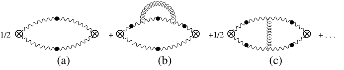
FIG. 3.: Resummed tree-level (a) and one-loop (b,c) diagrams contributing to the mean-square part of the Polyakov loop correlation. Here the wavy lines with a dot represent static longitudinal propagators while the transverse ones have been drawn as springs. Diagrams with vanishing next-to-leading order contribution have been omitted. Subtraction of the Debye mass counterterm is understood to be included in diagram (b). With a finite magnetic mass, there is also a seagull-type self-energy insertion to be added to (b).

The one-loop resummed correction to the mean-square correlation, $f^{(1)}_{\rm m.s.}$ is given by the remaining diagrams of Fig. 3. Inspecting first large $x\equiv m_{0}r$, one obtains[36]

$$f^{(0)+(1)}_{\rm m.s.}/f^{(0)}_{\rm m.s.}\equiv F(x)$$ (33)

$$= 1+\frac{\sqrt{3N^{\prime}}g}{2\pi}\left\{x(-\frac{1}{2}\ln x-\ln 2-\frac{\gamma}{2}+\frac{3}{2})+O(\ln x)\right\}$$ (34)

with $\gamma$ being Euler’s constant and $N^{\prime}$ as defined in Eq. (9). The correction terms that are linear in $x$ could be absorbed by a shift of the lowest order Debye mass $m_{0}^{2}\to m_{0}^{2}+\delta m^{2}$, but there is also a term proportional to $x\ln x$, which, if exponentiated, would lead to a potential that falls off faster than any Yukawa potential squared. Closer inspection of the Feynman diagrams[16] reveals, however, that the contributions $\propto x\ln x$ arise from singularities in momentum space which are strongly sensitive to the magnetic mass scale.

Indeed, introducing again a small magnetic mass $m_{\mathrm{m}}$ (see the appendix for details) changes the result (33) qualitatively for $x\gg m/m_{\mathrm{m}}$. The term $\propto x\ln x$ contributed by diagram 3b arises from a branch singularity coinciding with a double pole at ${\bf k}^{2}=-m^{2}$. A magnetic mass $m_{\mathrm{m}}$ separates these singularities and instead leads to a term linear in $x$. Its coefficient is given by the next-to-leading order correction to the Debye mass as derived from the gauge-independent pole of the gluon propagator in Sect. 2,

$$F^{(b)}(x)=\frac{\sqrt{3N^{\prime}}g}{2\pi}\left\{-x\left[(1-\frac{m_{\mathrm{m}}^{2}}{4m^{2}})\ln\frac{2m+m_{\mathrm{m}}}{m_{m}}-\frac{1}{2}-\frac{m_{\mathrm{m}}}{2m}\right]+O(x^{0})\right\}$$ (35)

The term $\propto x\ln x$ contributed by diagram 3c comes from a simple pole coinciding with a branch singularity at ${\bf k}^{2}=-4m^{2}$. A small magnetic mass replaces the pole by two neighbouring branch singularities[16], yielding

$$F^{(c)}(x)=\frac{\sqrt{3N^{\prime}}g}{2\pi}\left\{\frac{m^{2}}{m_{\mathrm{m}}^{2}}(\ln\frac{2m_{\mathrm{m}}x}{m}+\gamma)+O(m/m_{\mathrm{m}})\right\},$$ (36)

which grows only logarithmically at large $x$.

In these results, the unphysical gauge modes have been made massive, too. If they were kept massless, they would contribute gauge-parameter dependent terms proportional to $x$ to both $F^{(b)}$ and $F^{(c)}$ with opposite sign, leaving their sum unchanged. Absorbing all the linear terms of $F(x)$ by a shift of the Debye mass implies $F(x)\to F(x)+x{\delta m^{2}}/(mm_{0})$, thus leads to exactly the same next-to-leading order result for the Debye mass as from the gauge-independent pole of the gluon propagator, Eq. (18).

In order to inspect the PLC screening function in more detail we shall need the form of $F(x)$ also for moderate values of $x$. For $x\ll m/m_{\mathrm{m}}$, the complete correction to the pre-exponential screening function $F(x)$ of Eq. (33) reads[36]

$$F(x) = 1+\frac{\sqrt{3N^{\prime}}g}{2\pi}x\biggl{\{}-\frac{1}{2}\ln x-\ln 2-\frac{\gamma}{2}+\frac{3}{2}$$ (38)

$$-\frac{1}{2}g(2x)+\frac{\ln(2x)+\gamma}{x}+\frac{1}{2}e^{4x}{\rm Ei}(-4x)-\frac{1}{x}e^{2x}{\rm Ei}(-2x)\biggr{\}}$$

where Ei($x$) is the exponential integral[38], $x\equiv m_{0}r$, and

$$g(x)=\int_{0}^{\infty}\frac{dz}{z+1}e^{-xz}\ln\frac{z+2}{z}.$$ (39)

For large $x$, $g(x)\sim\ln(x)/x.$

Including the magnetic mass $m_{\mathrm{m}}$ makes a difference for $x\gtrsim m/m_{\mathrm{m}}$ and we instead obtain

$$F(x) = 1+\frac{\sqrt{3N^{\prime}}g}{2\pi}\frac{m_{0}}{m}\biggl{\{}\ell(\bar{x})-\frac{\bar{x}}{2}g(2\bar{x})+\bar{x}h(2\bar{x})+\frac{\bar{x}}{2}h(4\bar{x})$$ (43)

$$+\frac{\mu^{2}}{4}\ln\frac{2+\mu}{\mu}+(1-\frac{\mu^{2}}{4})(1-e^{-\mu\bar{x}})\left(\frac{1}{\mu}+\frac{1}{2+\mu}\right)$$

$$+e^{-\mu\bar{x}}\biggl{[}-(1-\frac{\mu^{2}}{4})\bar{x}\left\{h(\mu\bar{x})+h((2+\mu)\bar{x})\right\}$$

$$\qquad+(1+\frac{\mu^{2}}{4})\left\{h(\mu\bar{x})-h((2+\mu)\bar{x})\right\}+\ln\frac{2+\mu}{\mu}\biggr{]}\biggr{\}},$$

where $\bar{x}=mr=xm/m_{0}$ and $\mu=m_{\mathrm{m}}/m$. We have further introduced

$$h(x)\equiv e^{x}{\rm Ei}(-x)$$

and the function

$$\ell(x)\sim\cases{{x\over 2}(\ln(x)+\gamma)&for $x\ll 1/\mu$\cr\mu^{-2}\ln(x)&for $x\gg 1/\mu$\cr}$$ (44)

which we approximate by

$$\ell(x)\approx\frac{x}{2+\mu^{2}x}(\ln(x)+\gamma).$$ (45)

In Fig. 4 the screening function $F(x)\exp(-2xm/m_{0})$ is plotted logarithmically for the cases without and with a magnetic mass for the parameters used in Sect. 2. In order to get a notion of the uncertainties of the perturbative calculations, the next-to-leading order Debye mass $m$ is evaluated both fully self-consistently (solving the nonlinear equation defined by Eq. (18)) and strictly perturbatively (replacing $m\to m_{0}$ in all quantities that are already of relative order $g$). One finds that for large $x$ the dominant feature is exponential decay determined by the value of $m$. At small up to moderate distances the pre-exponential function is almost equally important. Notice that the effective Debye mass given by the slope of the tangent to the curves of Fig. 4 is generally smaller than the asymptotic value.

FIG. 4.: The logarithm of the screening function $S_{\rm PLC}=F(x)\exp(-2xm/m_{0})$ of the Polyakov loop correlation for $t\equiv g\sqrt{3N^{\prime}}/8=0.25$, both without and with a magnetic mass. The short-dashed curve gives the case without a magnetic mass and $m=m_{0}$, the full lines correspond to $m_{\mathrm{m}}/m_{0}=0.25$. The upper full line is for $m$ from a fully self-consistent evaluation of Eq. (18), the lower one for a strictly perturbative one as discussed in the text. The long-dashed line marks the classical result, $\ln S=-2x$.

For the range of $x$ covered by Fig. 4, the dependence of the screening function on the value of the magnetic mass is predominantly through the next-to-leading order value of the Debye mass rather than the explicit dependence of $F(x)$ on $m_{\mathrm{m}}$. The latter dependence becomes relevant only for $x\gg 1/\mu$, but there the perturbative result breaks down at some point, for $F(x)$ also grows $\gg 1$.

VI Screening with $A_{0}$ condensate

It has been speculated[39, 40] that the infrared divergences in the static sector of high-temperature nonabelian gauge theories cause the zero mode of $A_{0}$ to develop a vacuum expectation value which breaks SU($N$) down to U(1)^N-1. Nadkarni[40] has considered the effects of this scenario on chromoelectric screening in ring-resummed perturbation theory. From calculations in a unitary (diagonal) gauge, he suspected a strong modification of the Debye mass.

In the diagonal gauge, where $A_{0}$ only involves the diagonal generators of SU(N), correlation functions of the former correspond to the gauge invariant correlations of the eigenvalues of the Polyakov loop operator. The zero mode of $A_{0}$ is restricted to $\hat{v}+\epsilon^{\hat{a}}T^{\hat{a}}$ where $T^{\hat{a}}$ are the diagonal generators and $\hat{v}$ is the diagonal vacuum expectation value. In this parametrization, a nonvanishing $\hat{v}$ gives mass to the off-diagonal transverse static gluons $\tilde{A}$, which couple to the electrostatic fluctuations $\hat{\epsilon}$ through

$${\rm tr}[\tilde{A},\hat{v}+\hat{\epsilon}]^{2},$$

but there is no coupling between two electrostatic potential with only one transverse gluon. Since this was the only vertex in the next-to-leading order calculations in covariant and Coulomb gauges, it was maintained in Ref. [40] that all the results $\Pi_{00}\propto gm^{2}$ were pure gauge artefacts. However, by inspecting the perturbative series in diagonal gauge, one finds that it ceases to exist for $\hat{v}\to 0$. Denoting the mass acquired by the off-diagonal transverse static fields by $\mu=cg^{2}T$, where the value of $c$ is not determined by perturbation theory, the loop expansion parameter turns out to be $1/c$, which diverges in the symmetric limit. Hence, no statement can be made for the latter.

Nevertheless, with $c$ sufficiently large, the perturbation theory in diagonal gauge again makes sense and is in fact rather different from the case of no $A_{0}$ condensate. The correlation of two $\hat{\epsilon}$ operators is manifestly gauge invariant by virtue of its relation to the Polyakov loop eigenvalues. In Ref. [40] this correlation was considered at resummed one-loop order only in the limit $k^{2}\ll\mu^{2}$. With the Feynman rules derived in Ref. [40] it is straightforward to obtain the complete expression, which reads

$$\Pi_{00}(0,k)=m_{0}^{2}-\frac{\mu^{2}}{c\pi}\biggl{\{}1+\left(2+\frac{k^{2}}{\mu^{2}}+\frac{k^{4}}{4\mu^{4}}\right)\frac{\mu}{k}\arctan\frac{k}{2\mu}+\frac{k^{2}}{2\mu^{2}}\biggr{\}}.$$ (46)

For small $k$ this coincides with the result given in Ref. [40].

The analytic structure of Eq. (46) is quite different from the ones we have encountered before. Because the correction term in Eq. (46) is negative for large $k$ and grows $\sim k^{3}$, there is generally a pole of $(k^{2}+\Pi_{00}(0,k))^{-1}$ on the real $k$-axis. This is of course the dominant singularity for large distances and, taking the principal value, it would imply an oscillatory behaviour $\sim\cos(\lambda r)/r$. In fact, the residue is such that it even may start out repulsive at small distance, as shown in Fig. 5. However, this phenomenon is linked with the behaviour of the correction term in Eq. (46) at large values of $k/\mu$, where it blows up due to the unfavourable large-momentum behaviour of the gluon propagator in the unitary diagonal gauge. Judging from Eq. (46), the new perturbation series breaks down for $(k/\mu)^{3}\gtrsim c(m/\mu)^{2}$, which is in fact the region where the pole on the real axis arises. Since the other contributions to the screening function are suppressed at large $k/\mu$, it seems reasonable to just exclude the contribution of the pole on the real axis while keeping the other analytic structures at smaller $k$. This can easily be done by a different choice of the integration contour in Eq. (5).

FIG. 5.: The logarithm of the screening function $S(x)$ of the Polyakov loop eigenvalue correlation in the case of a nonzero $A_{0}$ condensate with $c=1$ and $\mu/m_{0}=0.25$, where $S(x)$ is normalized such that $S_{\rm cl.}=\exp(-x)$. The short-dashed curve gives the oscillatory behaviour when the pole on the real axis is included (see text), which starts out with a reversed (repulsive) sign. The full curve is the result upon subtraction of the contribution from the real pole, and the long-dashed line marks the the classical screening function.

With $\mu>m_{0}/2$ the only singularity is then the one at $k\approx\pm im_{0}$, so the asymptotic behaviour would be the classical one with only small corrections. However for $\mu<m_{0}/2$, which should be fulfilled at least with sufficiently small $g$, there is a branch cut on the imaginary axis superseding the original pole at $k=\pm im_{0}$. Hence, in this case, the magnetic mass scale is the dominant one in the asymptotic behaviour of the electric correlations. However, the imaginary part of $(k^{2}+\Pi_{00}(0,k))^{-1}$ along the cut is strongly peaked at $k\approx\pm im_{0}$, so this dominance of the magnetic scale will occur only at very large distances. At intermediate distances the effective Debye mass is smaller than but close to the classical one, as shown in Fig. 5 by the plot where the real pole contribution has been subtracted.

Altogether the resummed one-loop result for Debye screening with an $A_{0}$ condensate appears more uncertain than with the conventional vacuum. The entire correction term now is proportional to the coefficient $c$ of the magnetic mass of the off-diagonal transverse gluons. The value of $c$ is inherently nonperturbative like the value of the magnetic mass which was invoked in the previous sections, but there the dependence was only logarithmic. A large value of $c$ would provide a small loop expansion parameter of the new perturbation series obtained in the diagonal gauge, at least for sufficiently small momenta, but one can only expect $c\sim 1$.

VII Comparison with lattice simulations

Recently, high-precision lattice simulations of the Polyakov loop correlation in pure SU(2) gauge theory have been performed by Irbäck et al.[41]. These simulations employ temperatures up to nearly 8 times the critical temperature so that one may hope that perturbation theory becomes applicable. Moreover, in SU(2) there exist also some (rather old) lattice results on the value of the hypothetical magnetic screening mass, so we can combine these results to test the various perturbative estimates for next-to-leading order correction to Debye screening as presented in the previous sections, in which we had put in a magnetic screening mass by hand.

There exist also some results for SU(3), both without[42, 43] and with quarks[44], but the corresponding lattice simulations have achieved less precision and involve smaller values of $T/T_{c}$. Because of the latter, one has to expect more pronounced nonperturbative effects so that there is less chance for making contact with our perturbative considerations. Also, most of the lattice results for the magnetic mass, which is a crucial input in our perturbative estimates, have been obtained in pure SU(2).

We shall therefore concentrate on the results given in Ref. [41] and compare them with our various perturbative estimates. The lattice simulations of magnetic screening in pure SU(2) gauge theory[45] have given $m_{\mathrm{m}}=0.27(3)g^{2}T$, which is consistent with a recent semiclassical result by Biró and Müller [46] and also with a recent result from one-loop resummed gap equations in a non-linear sigma model for the magnetic mass term[47]. In what follows we shall plug in this value for the magnetic mass into our perturbative result for the next-to-leading order Debye mass (18) with the above error and evaluate it both strictly perturbatively and fully self-consistently. As discussed at the end of Sect. 2, in the strictly perturbative case we only resum the classical (HTL) Debye mass $m_{0}$ whereas in the second case we resum the full $m$, solving the resulting nonlinear equations for $m$ numerically. The variation of the results will serve us as a crude measure for the uncertainties of the resummed one-loop calculation.

In Ref. [41], the Polyakov loop correlation has been measured for lattice sizes $4\times 24^{3}$ at $g_{0}^{2}=1.43$ and $4\times 32^{4}$ at $g_{0}^{2}=1.33$, at distances of up to 8 lattice units. In order to make contact with perturbation theory, the coupling constant has to be renormalized. This is done at short distances, that is, at the smallest available distance of one lattice spacing, yielding $g^{2}\approx 1.28$ and $g^{2}\approx 1.19$, respectively. The smaller value of the coupling, which pertains to the larger lattice, corresponds to the rather high temperature $T/T_{c}\approx 7.8$ according to recent work by Fingberg et al.[48]. With this renormalised value of $g$, Eq. (18) yields for $m_{\mathrm{m}}/g^{2}T=0.27\pm 0.03$

$$\frac{m}{m_{0}}=\cases{1.22&$\mp 0.02$\cr 1.36&$\mp 0.04$\cr},$$ (47)

where the upper and lower lines correspond to perturbative and self-consistent evaluation, respectively. (With the larger value of $g$ the above values are almost unchanged.)

A screening mass has been extracted from the lattice data by fitting the unsubtracted PLC to the mean-square behaviour of Eq. (32) at distances of 4 to 8 lattice spacings. For both lattices, this corresponds to values of $x\approx 0.9\ldots 1.8$. Although these are not very large values, the mean-square approximation is probably quite good in SU(2), since there the next important correction term associated with 3 gluon exchange vanishes[36]. The results reported in Ref. [41] are

$$\frac{m}{m_{0}}=\cases{1.11(5)&for $g^{2}\approx 1.28$\cr 1.14(4)&for $g^{2}\approx 1.19$\cr}$$ (48)

i.e., a significant enhancement of the Debye screening mass over its classical value, which is even more pronounced for the smaller coupling corresponding to the higher temperature.

However, for the moderate values of $x\approx 1\ldots 2$ covered by the lattice calculations these numbers cannot yet be compared with the perturbative results which refer to the asymptotic behaviour. As we have seen in Sect. 5, it is important to take the pre-exponential screening functions into account when attempting to identify the asymptotic screening mass. From Fig. 4 it is clear that fitting the classical function $(e^{-mr}/r)^{2}$ on a restricted range of $x$ will underestimate $m$. In Fig. 6 the lattice data are compared with the perturbative results of Sect. 5 for the screening function $F(x)\exp(-2xm/m_{0})$. Fitting straight lines in this logarithmic plot gives an effective screening mass which reads

$$\frac{m_{eff.}}{m_{0}}=\cases{1.16(9)&PLC with $m_{\mathrm{m}}$ and Debye mass from Eq.~{}(\ref{mprp})\cr 0.97&PLC without magnetic mass and $m=m_{0}$\cr}$$ (49)

where the error gives the full variation caused by both the quoted error of the magnetic mass and the spread from a perturbative vs. self-consistent evaluation of the one-loop formulae. The PLC result without a magnetic mass thus leads to a slightly diminished effective Debye mass as compared with the classical value. On the other hand, the increase of the Debye mass according to Eq. (18) is not completely compensated by the curvature of $F(x)$ and leads to an effective Debye mass significantly larger than the classical value, in accordance with the lattice data. As concerns the magnitude of the screening function, the lattice data lie in between the perturbative results with and without a magnetic mass.

FIG. 6.: The logarithm of the screening function $F(x)\exp(-2xm/m_{0})$ of the Polyakov loop correlation in the range of $x\equiv m_{0}r$ covered by the lattice calculations of Ref. [41]. The long-dashed straight line gives the classical result. The short-dashed curve gives the one-loop resummed result for the mean-square contribution prior to the introduction of a magnetic mass. The full lines give the range of the results which include a magnetic mass $m_{\mathrm{m}}=0.27g^{2}T$. The upper and lower full line correspond to the upper and lower value of the Debye mass $m$ in Eq. (47), respectively. The lattice data for the connected Polyakov loop correlation are given by the thick dots. The error bars as reported in Ref.[41] are negligible except for the last two data points.

All of the above numbers depend crucially on the value of the renormalized coupling constant associated with the bare one on the lattice. So far we have followed the procedure of Ref. [41], where the former was determined by matching the short-distance behaviour to the tree-level result of the bare perturbation theory. Using instead the resummed tree-level result which includes the leading-order Debye mass necessarily gives a different renormalized coupling because one cannot go to smaller distances than one lattice spacing. In the case of the larger lattice and higher temperature, the latter procedure increases $g_{0}^{2}=1.33$ to $g^{2}_{R}\approx 1.53$, while previously the renormalized coupling was diminished. With this larger value of $g_{R}$, the results in Eq. (49) are only insignificantly increased, yielding now

$$\frac{m_{eff.}}{m_{0}}=\cases{1.18(11)&PLC with $m_{\mathrm{m}}$ and Debye mass according to Eq.~{}(\ref{d})\cr 0.98&PLC without magnetic mass and $m=m_{0}$\cr}$$ (50)

whereas the lattice result (48) is reduced to $m/m_{0}=1.00(4)$. Apparently this is in better agreement with the perturbative result prior to the introduction of a magnetic mass, but by directly comparing the complete screening functions with the lattice data, redone in Fig. 7, the case with a magnetic mass and an enhanced Debye mass from Eq.(18), seems to be clearly favoured.

FIG. 7.: Same as Fig. 6, but with a renormalized coupling of $g^{2}\approx 1.53$, which is obtained by matching the short-distance behaviour to the resummed (rather than bare) tree-level result.

Finally we briefly turn also to the case of an $A_{0}$ condensate, where we have encountered a rather different analytic structure of the screening function. There the theoretical uncertainty is much greater, because the loop expansion parameter $1/c$ is always $\gtrsim 1$ (with the above parameters $1/c\approx 4$). In Sect. 6 we have found an oscillatory behaviour that started out repulsive, but we have argued that this result is not perturbatively stable. After discarding this part of the result, there remained a contribution from a branch cut at $k=\pm 2im_{\mathrm{m}}$ instead of $\pm im$. For very small coupling, this should be a distinctive feature, at least at sufficiently large distances. However, the lattice results involve only moderate values of $x$ and furthermore, for the coupling constant that was used in the above lattice simulations and the assumed magnetic mass, we have $2m_{\mathrm{m}}/m=0.7(2)$. For large $x$ this suggests a diminished Debye screening mass, but at the not so large $x$ for which lattice data exist, the effective screening mass may be different. Indeed, the screening function displayed in Fig. 5 has positive curvature (in contrast to those of Fig. 4), so for smaller $x$ the effective screening mass now becomes larger. With the lattice parameters, the one-loop result yields $m_{eff.}/m_{0}\approx 1.05$, i.e. even a slight enhancement compared to the classical Debye mass, thus going in the right direction. However, as has been shown recently[51], in the case of a nonvanishing $A_{0}$ condensate the leading term in the PLC is not the mean-square contribution of Eq. (32) but one which involves only one power of the usual Yukawa-type potential. Fitting the latter behaviour to the lattice results of Ref. [41] gives $m/m_{0}\approx 3.4(1)$ ($\approx 3.0(1)$ if the larger value of the renormalized coupling is used), which is far off from the perturbative result.

In view of the largeness of the coupling and the uncertainty associated with the treatment of the magnetic mass, one certainly cannot expect next-to-leading order results to be really accurate, but the agreement of the lattice data with the screening function of the symmetric scenario with a magnetic mass $m_{\mathrm{m}}\sim g^{2}T/4$ and the enhanced Debye mass according to Eq. (18) is in fact surprisingly good. The range of $x$ covered by the existing lattice calculations is however too small to really pin down the actual asymptotic behaviour. Even the qualitatively different asymptotics suggested by the TAG result, which shows oscillatory behaviour with a repulsive power-law tail[14], would manifest itself only for $x$ considerably greater than 2. However, lattice simulations at larger values of $x$ are probably prohibitively difficult, since the statistical errors increase very quickly with $x$. On the other hand, progress with (resummed) perturbation theory seems only possible through a better understanding of the nonperturbative magnetic sector of thermal nonabelian gauge theories.

In this appendix some details to the evaluation of the PLC screening function are given when a magnetic screening mass is included, supplementing the calculations contained in the appendix of Ref. [36].

$F^{(b)}$, introduced in Sect. 5 and corresponding to the function $f_{I}$ of Ref. [36], is given by

$$F^{(b)}=8\pi re^{mr}\int\frac{d_{3}{\bf k}\,e^{-i{\bf k}\cdot{\bf r}}}{({\bf k}^{2}+m^{2})^{2}}\left(\delta m^{2}-\delta\Pi_{00}(0,k)\right)$$ (51)

where $d_{3}{\bf k}\equiv{d^{3-2\varepsilon}k}/{(2\pi)^{3-2\varepsilon}}$ and

$$\delta\Pi_{00}(k_{0}=0,{\bf k})=g^{2}NT\int d_{3}{\bf p}\,\biggl{\{}\frac{1}{{\bf p}^{2}+m^{2}}+\frac{1}{{\bf p}^{2}+m_{\mathrm{m}}^{2}}$$ (52)

$$\qquad+\frac{2(m^{2}-m_{\mathrm{m}}^{2}/2-{\bf k}^{2})}{{\bf p}^{2}({\bf q}^{2}+m^{2})}+(\alpha-1)({\bf k}^{2}+m^{2})\frac{{\bf p}^{2}+2{\bf p}{\bf k}}{({\bf p}^{2}+m_{\mathrm{m}}^{2})^{2}({\bf q}^{2}+m^{2})}\biggr{\}},$$ (53)

with ${\bf q}={\bf p}+{\bf k}$.

This leads to

$$F^{(b)} = mr\frac{\delta m^{2}}{m^{2}}+\frac{g^{2}NT}{2\pi m}\biggl{\{}\frac{(m+m_{\mathrm{m}})r}{2}+4\pi m(1-\alpha)\int d_{3}{\bf l}\,\frac{(1-e^{i{\bf l}\cdot{\bf r}})}{({\bf l}^{2}+m_{\mathrm{m}}^{2})^{2}}$$ (55)

$$+\frac{i}{\pi}\int_{C}dz\,e^{-mrz}\frac{z^{2}+2z+2-\mu^{2}/2}{z^{2}(2+z)^{2}}\ln\frac{\mu-z}{2+\mu+z}\biggr{\}},$$

where the contour $C$ encircles the positive real axis and $\mu\equiv m_{\mathrm{m}}/m$.

The contour integral in (55) receives contributions from a pole at $z=0$ and a branch cut starting at $z=\mu$, which thus is separated from the pole by the finite magnetic mass. The contribution from the pole reads

$$i\pi\biggl{\{}(1-\mu^{2}/4)\left[-mr\,\ln\frac{\mu}{2+\mu}-\frac{1}{\mu}-\frac{1}{2+\mu}\right]+\frac{\mu^{2}}{4}\ln\frac{\mu}{2+\mu}\biggr{\}},$$ (56)

and the one from the cut

$$i\pi\biggl{\{}(1-\mu^{2}/4)\left[e^{-m_{\mathrm{m}}r}\left(\frac{1}{\mu}+\frac{1}{2+\mu}\right)+mr\,{\rm Ei}(-m_{\mathrm{m}}r)+mr\,e^{2mr}\,{\rm Ei}(-(2+\mu)mr)\right]$$ (57)

$$\qquad-\frac{\mu^{2}}{4}{\rm Ei}(-m_{\mathrm{m}}r)+\frac{\mu^{2}}{4}e^{2mr}\,{\rm Ei}(-(2+\mu)mr)\biggr{\}}.$$ (58)

In general covariant gauge and with a magnetic mass, $F^{(c)}$, which corresponds to the function $f_{II}$ of Ref. [36], reads

$$F^{(b)}=g^{2}NT\left\{-2(1-\alpha)I_{2}+(4\pi r)^{2}e^{2mr}\left[4I_{3}-I_{4}-2I_{5}\right]\right\}$$ (59)

with

$$I_{3} = \int\frac{d_{3}{\bf k}_{1}\,d_{3}{\bf k}_{2}\,d_{3}{\bf l}\,e^{-i({\bf k}_{1}-{\bf k}_{2})\cdot{\bf r}}}{({\bf k}_{1}^{2}+m^{2})[({\bf k}_{1}+{\bf l})^{2}+m^{2}]({\bf k}_{2}^{2}+m^{2})({\bf l}^{2}+m_{\mathrm{m}}^{2})}$$ (60)

$$I_{4} = \int d_{3}{\bf k}\,e^{-i{\bf k}\cdot{\bf r}}\left[\int\frac{d_{3}{\bf l}}{[({\bf l}+{\bf k})^{2}+m^{2}]({\bf l}^{2}+m^{2})}\right]^{2}$$ (61)

$$I_{5} = \int\frac{d_{3}{\bf k}\,e^{-i{\bf k}\cdot{\bf r}}({\bf k}^{2}+2m^{2}-m_{\mathrm{m}}^{2}/2)\,d_{3}{\bf p}\,d_{3}{\bf q}}{[({\bf p}-{\bf q})^{2}+m_{\mathrm{m}}^{2}]({\bf p}^{2}+m^{2})({\bf q}^{2}+m^{2})[({\bf p}+{\bf k})^{2}+m^{2}][({\bf q}+{\bf k})^{2}+m^{2}]}.$$ (62)

The gauge-parameter dependent parts of $F^{(c)}$ exactly cancel those of $F^{(b)}$. The integral appearing therein yields

$$I_{2}\equiv\int d_{3}{\bf l}\frac{(1-e^{i{\bf l}\cdot{\bf r}})}{({\bf l}^{2}+m_{\mathrm{m}}^{2})^{2}}=\frac{1}{8\pi m_{\mathrm{m}}}\left(1-e^{-m_{\mathrm{m}}r}\right),$$ (63)

so even separately these terms do not contribute to the linear terms in $r$ that constitute the next-to-leading order shift of the Debye screening mass if the unphysical gauge degrees of freedom are made massive; if they are kept massless, $I_{2}\to r/(8\pi)$, and these linear contributions cancel upon adding $F^{(b)}$ and $F^{(c)}$.

In Ref. [36] all of the above integrals were evaluated exactly in the case of a vanishing magnetic mass. With a finite magnetic mass, $I_{3}$ can still be calculated completely, which yields

$$I_{3} = \frac{ie^{-2mr}}{(4\pi r)^{2}8\pi^{2}m}\int_{C}\frac{dz\,e^{-mrz}}{z(2+z)}\ln\frac{\mu-z}{2+\mu+z}$$ (64)

$$= \frac{e^{-2mr}}{(4\pi r)^{2}8\pi m}\left[{\rm Ei}(-m_{\mathrm{m}}r)-e^{2mr}\,{\rm Ei}(-(2+\mu)mr)-\ln\frac{\mu}{2+\mu}\right].$$ (65)

$I_{4}$ is unchanged by the introduction of the magnetic mass and reads

$$I_{4}=\frac{e^{-2mr}}{(4\pi r)^{2}}\frac{r}{4\pi}g(2mr),$$ (66)

with $g$ as defined in Eq. (39).

$I_{5}$, with a finite magnetic mass, can be brought into the form

$$I_{5}=\int d_{3}{\bf k}\,e^{-i{\bf k}\cdot{\bf r}}({\bf k}^{2}+2m^{2}-m_{\mathrm{m}}^{2}/2)J(k)$$ (67)

where $J(k)$ is given by the double integral

$$J(k) = \frac{1}{32\pi^{2}}\int_{0}^{1}\frac{dx}{\sqrt{k^{2}x(1-x)+m^{2}}}$$ (68)

$$\times \int_{0}^{1}\frac{dy(1-2xy)}{[k^{2}+4(m^{2}+yW)]\sqrt{k^{2}xy(1-xy)+m^{2}+yW}}$$ (69)

where $$W(k,x)\equiv m_{\mathrm{m}}^{2}+2m_{\mathrm{m}}\sqrt{k^{2}x(1-x)+m^{2}}.$$ (70)

With $m_{\mathrm{m}}=W=0$,

$$J(k)=\frac{1}{16\pi^{2}k^{2}(k^{2}+4m^{2})}\ln\frac{k^{2}+4m^{2}}{4m^{2}},$$ (71)

which leads to

$$I_{5} = \frac{e^{-2mr}}{(4\pi r)^{2}}\frac{r}{8i\pi^{2}}\int_{C}\frac{dz\,e^{-2mrz}(1+4z+2z^{2})}{z(1+z)(2+z)}\ln[-z(2+z)]$$ (72)

$$= -\frac{e^{-2mr}}{(4\pi r)^{2}}\frac{r}{8\pi}\left[\ln(mr)+\gamma+2e^{2mr}\,{\rm Ei}(-2mr)+e^{4mr}\,{\rm Ei}(-4mr)\right].$$ (73)

As has been pointed out first in Ref. [16], a finite magnetic mass removes the pole at $k^{2}=-4m^{2}$ (corresponding to $z=0$) and replaces it by neighbouring branch singularities at $k^{2}=-4m^{2}$ and $k^{2}=-(2m+m_{\mathrm{m}})^{2}$. In the limit $\kappa^{2}=-k^{2}\to 4m^{2}$, $J(k)$ yields

$$J(k)\Big{|}_{k^{2}\to-4m^{2}}\sim\frac{1}{(16\pi mm_{\mathrm{m}})^{2}}\ln\frac{2m-\kappa}{4m}\ln\frac{4m^{2}-\kappa^{2}}{4m_{\mathrm{m}}^{2}},$$ (74)

which leads to the large distance behaviour

$$I_{5}\sim-\frac{e^{-2mr}}{(4\pi r)^{2}}\frac{m}{4\pi m_{\mathrm{m}}^{2}}(\ln 2m_{\mathrm{m}}r+\gamma),$$ (75)

up to terms that are down by powers of $m_{\mathrm{m}}/m$.

Putting everything together leads to Eq. (43), where the full function $I_{5}$ has been approximated in terms of the function $\ell(x)$ introduced in Eq. (45).

REFERENCES

- [1] J. Frenkel and J. C. Taylor, Nucl. Phys. B334 (1990) 199.
- [2] E. Braaten and R. D. Pisarski, Phys. Rev. Lett. 64 (1990) 1338; Nucl. Phys. B337 (1990) 569.
- [3] V. P. Silin, Zh. Eksp. Teor. Fiz. 38 (1960) 1577 [Sov. Phys. 11 (1960) 1136]; U. Heinz, Ann. Phys. (N.Y.) 161 (1985) 48; ibid. 168 (1986) 148; J.-P. Blaizot and E. Iancu, Nucl. Phys. B417 (1994) 608; P. F. Kelly, Q. Liu, C. Lucchesi and C. Manuel, Phys. Rev. Lett. 72 (1994) 3461.
- [4] G. Barton, Ann. Phys. (N.Y.) 200 (1990) 271; J. Frenkel and J. C. Taylor, Nucl. Phys. B374 (1992) 156.
- [5] E. Braaten and R. D. Pisarski, Phys. Rev. D42 (1990) 2156; ibid. D46 (1992) 1829; R. Kobes, G. Kunstatter and K. Mak, Phys. Rev. D45 (1992) 4632.
- [6] H. Schulz, Nucl. Phys. B413 (1994) 353.
- [7] R. R. Parwani, Phys. Rev. D45 (1992) 4695.
- [8] U. Kraemmer, A. K. Rebhan and H. Schulz, DESY-report 94-034 (1994), to appear in Ann. Phys. (N. Y.).
- [9] R. D. Pisarski, Phys. Rev. Lett. 63 (1989) 1129; V. V. Lebedev and A. V. Smilga, Physica A181 (1992) 187; C. P. Burgess and A. L. Marini, Phys. Rev. D45 (1992) R17; A. Rebhan, ibid. D46 (1992) 482; T. Altherr, E. Petitgirard and T. del Rio Gaztelurrutia, Phys. Rev. D47 (1993) 703.
- [10] R. Baier, H. Nakkagawa and A. Niégawa, Can. J. Phys. 71 (1993) 205; R. Pisarski, Phys. Rev. D47 (1993) 5589; S. Peigné, E. Pilon and D. Schiff, Z. Phys. C60 (1993) 455.
- [11] A. K. Rebhan, Phys. Rev. D48 (1993) R3967.
- [12] T. Matsui and H. Satz, Phys. Lett. 178B (1986) 416.
- [13] F. Cornu and Ph. A. Martin, Phys. Rev. A44 (1991) 4893.
- [14] R. Baier and O. K. Kalashnikov, Phys. Lett. B328 (1994) 450.
- [15] S. Peigné and S. M. H. Wong, preprint LPTHE-Orsay 94/46 (1994).
- [16] E. Braaten and A. Nieto, preprint NUHEP-TH-94-18 (1994).
- [17] H. A. Weldon, Phys. Rev. D26 (1982) 1394.
- [18] J. I. Kapusta, Finite Temperature Field Theory (Cambridge University Press, Cambridge, 1989).
- [19] T. Toimela, Z. Phys. C27 (1985) 289.
- [20] R. Kobes, G. Kunstatter and A. Rebhan, Phys. Rev. Lett. 64 (1990) 2992; Nucl. Phys. B355 (1991) 1.
- [21] E. S. Fradkin, Proc. of the Lebedev Institute 29 (1965) 6.
- [22] P. Arnold and O. Espinosa, Phys. Rev. D47 (1993) 3546.
- [23] M. Gell-Mann and K. A. Brueckner, Phys. Rev. 106 (1957) 364.
- [24] R. Baier, G. Kunstatter and D. Schiff, Phys. Rev. D45 (1992) 4381; Nucl. Phys. B388 (1992) 287.
- [25] A. Rebhan, Phys. Rev. D46 (1992) 4779.
- [26] A. K. Rebhan, to appear in the proceedings of the NATO Advanced Research Workshop “Electroweak Physics and the Early Universe”, March 1994, Sintra, Portugal.
- [27] A. D. Linde, Phys. Lett. B96 (1980) 289.
- [28] D. Gross, R. Pisarski and L. Yaffe, Rev. Mod. Phys. 53 (1981) 43.
- [29] L. Dolan and R. Jackiw, Phys. Rev. D9 (1974) 3320.
- [30] K. Kajantie and J. Kapusta, Ann. Phys. (N.Y.) 160 (1985) 477.
- [31] U. Heinz, K. Kajantie and T. Toimela, Ann. Phys. (N. Y.) 176 (1987) 218.
- [32] U. Kraemmer, M. Kreuzer, A. Rebhan and H. Schulz, Lect. Notes in Phys. 361 (1990) 285.
- [33] S. Carracciolo, G. Curci and P. Menotti, Phys. Lett. 113B (1982) 311.
- [34] K. James and P. V. Landshoff, Phys. Lett. B251 (1990) 167.
- [35] M. Kreuzer and H. Nachbagauer, Phys. Lett. B271 (1991) 155; H. Nachbagauer, Z. Phys. C56 (1992) 407.
- [36] S. Nadkarni, Phys. Rev. D33 (1986) 3738.
- [37] L. D. McLerran and B. Svetitsky, Phys. Rev. D24 (1981) 450.
- [38] I. S. Gradshteyn and I. M. Ryzhik, Table of Integrals, Series, and Products (Academic Press, Orlando 1980).
- [39] R. Anishetty, J. Phys. G 10 (1984) 423; J. Polonyi and H. W. Wyld, Illinois Report No. ILL-TH-85-23 (1985); K. J. Dahlem, Z. Phys. C29 (1985) 553; J. Boháčik, Phys. Rev. D42 (1990) 3554; M. Oleszczuk, in Hot Summer Daze, eds. A. Gocksch and R. Pisarski (World Sci., Singapore 1992).
- [40] S. Nadkarni, Phys. Rev. D34 (1986) 3904.
- [41] A. Irbäck, P. LaCock, D. Miller, B. Petersson and T. Reisz, Nucl. Phys. B363 (1991) 34.
- [42] M. Gao, Phys. Rev. D 41 (1990) 626.
- [43] L. Kärkkäinen, P. LaCock, D. E. Miller, B. Petersson and T. Reisz, Phys. Lett. B282 (1992) 121.
- [44] L. Kärkkäinen, P. LaCock, B. Petersson and T. Reisz, Nucl. Phys. B395 (1993) 733.
- [45] A. Billoire, G. Lazarides and Q. Shafi, Phys. Lett. 103B (1981) 450; T. A. DeGrand and D. Toussaint, Phys. Rev. D25 (1982) 526.
- [46] T. S. Biró and B. Müller, Nucl. Phys. A561 (1993) 477.
- [47] O. Philipsen, to appear in the proceedings of the NATO Advanced Research Workshop “Electroweak Physics and the Early Universe”, March 1994, Sintra, Portugal.
- [48] J. Fingberg, U. Heller and F. Karsch, Nucl. Phys. B392 (1993) 493.
- [49] J. Engels, F. Karsch and H. Satz, Nucl. Phys. B315 (1989) 419.
- [50] J. Engels, K. Mitrjushkin and T. Neuhaus, Nucl. Phys. B (Proc. Suppl.) 34 (1994) 298.
- [51] J. Boháčik and P. Prešnajder, Phys. Lett. B332 (1994) 366.