SPHALERONS AND STRINGS

Mark Hindmarsh

School of Mathematical and Physical Sciences,
University of Sussex,
Brighton BN1 9QH

INTRODUCTION

This work is based on a paper with Margaret James.${}^{\ref{HinJam94}}$ In it we showed that the dipole moment of the sphaleron has its origin in two components: a ring of electric current circulating around the edge of the sphaleron; and also two regions of opposite magnetic charge above and below the ring. This magnetic charge has a partly topological explanation, arising from the fact that the sphaleron is axisymmetric and parity invariant. Here, I shall make a few remarks that are complementary to our paper. Firstly, I discuss the definition of the electromagnetic field and its sources in the Standard Model, comparing ours with the better-known one of ’t Hooft.${}^{\ref{tHo74}}$ Both allow magnetic charges and currents, but ’t Hooft’s magnetic charge is designed purely to count zeroes of the Higgs field and is not a very satisfactory dynamical quantity. Secondly, I summarize the results of our paper,${}^{\ref{HinJam94}}$ which uses our definition of the electromagnetic field to look inside the sphaleron and find the distribution of charges and currents which give rise to its dipole moment. Finally, I go into a bit more detail about the resemblance between the sphaleron and Nambu’s “dumb-bell”${}^{\ref{Nam77}}$ – a segment of $Z$-string which connects a monopole to an antimonopole. It has been conjectured that the string segment is a kind of “stretched” sphaleron:${}^{\ref{Vac93},\ref{BarVacBuc94}}$ however, it is possible to estimate the Chern-Simons number $N_{\rm CS}$ using the topology of the Higgs field alone, providing the gauge is chosen correctly. In this gauge it can be shown that the string segment lacks a crucial twist in its field configuration that in the sphaleron results in $N_{\rm CS}={\mathchoice{{\textstyle{1\over 2}}}{1\over 2}{1\over 2}{1\over 2}}$.

ELECTROMAGNETISM IN THE STANDARD MODEL

In the Standard Model there is no unambiguous definition of the electromagnetic field. The first step, on which all agree, is to use a unit isovector

$$\hat{\phi}^{a}=\Phi^{{\dagger}}\sigma^{a}\Phi/|\Phi|^{2},$$ (1)

to project out the massless component of the gauge potential:

$$A_{\mu}=-W^{a}_{\mu}\hat{\phi}^{a}\sin\theta_{\rm W}+Y_{\mu}\cos\theta_{\rm W},$$ (2)

where $W^{a}_{\mu}$ and $Y_{\mu}$ are the SU(2) and U(1) gauge fields respectively. This reduces to the usual expression when the Higgs takes its conventional vacuum expectation value $\Phi=(0,1)^{\rm T}v/\sqrt{2}$, for then $\hat{\phi}^{a}=-\delta^{a}_{3}$. We can also project out the massless component of the gauge field strength tensor:

$$F^{\rm em}_{\mu\nu}=-F^{a}_{\mu\nu}\hat{\phi}^{a}\sin\theta_{\rm W}+F^{0}_{\mu\nu}\cos\theta_{\rm W}.$$ (3)

However, there is a remnant of the non-Abelian theory in which it is embedded, for the relationship between $F^{\rm em}_{\mu\nu}$ and $A_{\mu}$ does not take the simple form of ordinary electromagnetism. In fact,

$$F^{\rm em}_{\mu\nu}=\partial_{[\mu}A_{\nu]}+{\sin\theta_{\rm W}\over g}\left[\hat{\phi}^{a}\partial_{\mu}\hat{\phi}^{b}\partial_{\nu}\hat{\phi}^{c}-\hat{\phi}^{a}D_{\mu}\hat{\phi}^{b}D_{\nu}\hat{\phi}^{c}\right]\epsilon^{abc},$$ (4)

where $D_{\mu}\hat{\phi}^{a}=\partial_{\mu}+g\epsilon^{abc}W^{b}_{\mu}\hat{\phi}^{c}$. (A sign error in Ref. 1 has been corrected here.) This means that the Bianchi identity is not satisfied, and there is a magnetic current given by the right hand side of

$${\mathchoice{{\textstyle{1\over 2}}}{1\over 2}{1\over 2}{1\over 2}}\epsilon^{\mu\nu\rho\sigma}\partial_{\nu}F^{\rm em}_{\rho\sigma}=-{\mathchoice{{\textstyle{1\over 2}}}{1\over 2}{1\over 2}{1\over 2}}\sin\theta_{\rm W}\epsilon^{\mu\nu\rho\sigma}F^{a}_{\nu\rho}D_{\sigma}\hat{\phi}^{a}.$$ (5)

Note that $D_{\sigma}\hat{\phi}^{a}$ is orthogonal to $\hat{\phi}^{a}$, so that the magnetic current is comprised of gauge fields orthogonal both to the electromagnetic field and to the Z field, $F^{\rm Z}_{\mu\nu}=-F^{a}_{\mu\nu}\cos\theta_{\rm W}-F^{0}{\mu\nu}\sin\theta_{\rm W}$. In other words, magnetic currents in the Standard Model are made of W fields. W fields also make electric currents, for one can show that

$$\partial^{\nu}F^{\rm em}_{\mu\nu}=-\sin\theta_{\rm W}F^{a}_{\mu\nu}D^{\nu}\hat{\phi}^{a}.$$ (6)

The Higgs field does not contribute directly to this expression. This is to be expected, for the physical Higgs field is neutral.

A definition that many authors use is that of ’t Hooft, who gives the electromagnetic field as

$${\cal F}^{\rm em}_{\mu\nu}=F^{\rm em}_{\mu\nu}+{\sin\theta_{\rm W}\over g}\hat{\phi}^{a}D_{\mu}\hat{\phi}^{b}D_{\nu}\hat{\phi}^{c}\epsilon^{abc}.$$ (7)

The purpose of adding the extra term is to force the electromagnetic field to satisfy the Bianchi identity almost everywhere, for

$${\mathchoice{{\textstyle{1\over 2}}}{1\over 2}{1\over 2}{1\over 2}}\epsilon^{\mu\nu\rho\sigma}\partial_{\nu}{\cal F}^{\rm em}_{\rho\sigma}={\sin\theta_{\rm W}\over 2g}\epsilon^{\mu\nu\rho\sigma}\partial_{\nu}\hat{\phi}^{a}\partial_{\rho}\hat{\phi}^{b}\partial_{\sigma}\hat{\phi}^{c}\epsilon^{abc}.$$ (8)

The right hand side of this expression vanishes everywhere except along world lines around which $\phi^{a}$ takes “hedgehog” configurations.${}^{\ref{tHo74}}$ Thus the ’t Hooft magnetic flux out of a closed surface serves merely to count zeroes of the Higgs field.

The two expressions (3) and (7) agree in the Higgs vacuum, where $D_{\mu}\hat{\phi}^{a}=0$. Away from the vacuum they disagree, and there is no absolute standard by which to judge them. However, the first definition has the advantage that the energy density in the magnetic field is always $F^{\rm em}_{ij}{F^{\rm em}}^{ij}$, whereas the ’t Hooft magnetic field energy density must be corrected with derivatives of the isovector $\hat{\phi}^{a}$. Furthermore, there seems no reason to try and satisfy the Bianchi identities almost everywhere – we know that there is magnetic charge in non-Abelian theories, so why not have it spread out and created out of physical fields of the theory?

Accordingly, we shall use definition (3) in what follows. With it, we can look inside the sphaleron and find that at non-zero Weinberg angle the W fields do provide both electric currents and magnetic charges.

INSIDE THE SPHALERON

The sphaleron at zero Weinberg angle is a spherically symmetric solution of the classical field equations of the Standard Model, which can be written in the following form, in the radial gauge $W_{r}=0$:

$$\Phi=U(\hat{\mbox{\boldmath$x$}})\pmatrix{0\cr 1\cr}h(r)\frac{v}{\sqrt{2}},\qquad W=-{2i\over g}dUU^{-1}f(r),$$ (9)

where $U=i\hat{\mbox{\boldmath$x$}}\cdot\mbox{\boldmath$\sigma$}\sigma_{2}$. The isovector field around this configuration is

$$\hat{\phi}^{a}=2\hat{x}^{a}\hat{x}^{3}-\delta^{a3}.$$ (10)

This field is illustrated in Figure 1. In the core of the sphaleron, the fields leave the vacuum and there is non-zero $D_{i}\Phi$ and $F^{a}_{ij}$. The spherical symmetry of the energy density is in fact guaranteed by the custodial SU(2) symmetry of the Standard Model, so it is understandable that when $\theta_{\rm W}\neq 0$ the equal-energy contours of the sphaleron solution become prolate.${}^{\ref{KleKunBri92}}$ The sphaleron also develops a magnetic dipole moment, which has been calculated perturbatively in the small $\theta_{\rm W}$ limit,${}^{\ref{KliMan84},\ref{Jam92}}$ and also numerically for general values of $\theta_{\rm W}$.${}^{\ref{KleKunBri92}}$

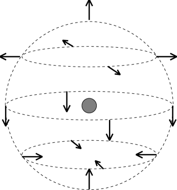
Figure 1: Isovector field configuration $\hat{\phi}^{a}$ around the sphaleron at $\theta_{\rm W}=0$.

With the definition (3) of the electromagnetic field we can understand this dipole moment in terms of magnetic charges and electric current defined in a gauge invariant way. Let us evaluate them to first order in $\theta_{\rm W}$, where the perturbation to the background configuration does not appear. Using equations (5) and (6) we find that the magnetic charge density $\tilde{\rho}$ and the electric current $J_{i}$ are given by

$$\tilde{\rho}=\frac{g^{\prime}}{g}8\cos\theta\frac{f^{\prime}(1-f)}{gr^{2}},\qquad\mbox{\boldmath$J$}=\frac{g^{\prime}}{g}8\sin\theta\frac{f(1-f)^{2}}{gr^{4}}{\hat{\mbox{\boldmath$e$}}_{\varphi}},$$ (11)

where ${\hat{\mbox{\boldmath$e$}}_{\varphi}}$ is the azimuthal unit vector in spherical polar coordinates. The magnetic dipole moment of this charge and current distribution is

$$\frac{g^{\prime}}{g}\frac{32\pi}{3g}\int_{0}^{\infty}\left[rf^{\prime}(1-f)+f(1-f)^{2}\right]dr.$$ (12)

When the function $f$ is found numerically,${}^{\ref{Jam92}}$ we find that the charge and the current contribute 70% and 30% respectively to the dipole moment. Moreover, this expression can be shown to be identical to that derived by Klinkhamer and Manton.${}^{\ref{KliMan84}}$ The total magnetic charge in each hemisphere is $4\pi\theta_{\rm W}/g$, which is $\theta_{\rm W}$ multiplied by the charge of a ’t Hooft-Polyakov SU(2) monopole${}^{\ref{tHo74},\ref{Pol74}}$. Indeed, the isovector field configuration looks as if it could be the Higgs field around a monopole-antimonopole pair in the Georgi-Glashow model. This might make one wonder if the presence of the magnetic charge was in some way topological.

The topology lies in the subspace of field configurations which are restricted to be axisymmetric and parity invariant. On the equatorial plane these configurations have $\hat{\phi}^{a}$ constant, which can be chosen to be $-\delta^{a}_{3}$, and the SU(2) gauge field takes the form${}^{\ref{KleKunBri92}}$

$$gW_{i}dx^{i}=if_{1}(r)(-\sin\varphi\sigma_{1}+\cos\varphi\sigma_{2})d\theta+if_{2}(r)\sigma_{3}d\varphi,$$ (13)

where $f_{1}$ and $f_{2}$ are functions which tend to 1 at infinity and vanish at the origin. The magnetic charge $\tilde{Q}$ in the region $z\geq 0$ can be expressed as an integral of the magnetic field over a surface consisting of a hemisphere at infinity $N$ plus the equatorial plane $E$:

$$\tilde{Q}_{z\geq 0}=\int_{N+E}dx^{i}B_{i}^{\rm em}.$$ (14)

Using the expression (4) for the electromagnetic field tensor, we see that the only contribution to this surface integral comes from the “non-Abelian” parts involving derivatives of the isovector field $\hat{\phi}^{a}$. On the equatorial plane, both $\partial_{i}\hat{\phi}^{a}$ and $\hat{\phi}^{a}D_{i}\hat{\phi}^{b}D_{j}\hat{\phi}^{c}\epsilon^{abc}$ vanish. Thus the magnetic charge $\tilde{Q}$ is given in terms of the integral

$$\tilde{Q}_{z\geq 0}={\sin\theta_{\rm W}\over g}\int_{N}\hat{\phi}^{a}\partial_{i}\hat{\phi}^{b}\partial_{j}\hat{\phi}^{c}\epsilon^{abc}.$$ (15)

Recall that $\hat{\phi}^{a}$ is constant on the boundary of the hemisphere: thus the hemisphere is effectively a 2-sphere, and integral on the right hand side of this equation measures the winding number of the isovector field around the unit sphere $\hat{\phi}^{2}=1$. Therefore, for axisymmetric, parity-invariant configurations, the magnetic charge in the region $z\geq 0$ is quantized in units of $4\pi\sin\theta_{\rm W}/g$. The same considerations apply to the region $z\leq 0$. The parity operation reverses magnetic fields, and so switches the sign of magnetic charge. Thus the charge in the other hemisphere must be equal and opposite.

SPHALERONS AND ELECTROWEAK STRINGS

The Standard Model contains another non-trivial classical solution, which is a vortex carrying Z-flux.${}^{\ref{Nam77},\ref{Vac92}}$ It is not topologically stable, and is dynamically stable only in the unphysical region $\sin\theta_{\rm W}\simeq 1$.${}^{\ref{JamPerVac93}}$ Because of their topological triviality, they can end, and Nambu${}^{\ref{Nam77}}$ showed that they terminate on monopoles, which have magnetic charge $\pm 4\pi\sin\theta_{\rm W}/g$. Nambu proposed that there was a massive long-lived excitation in the Standard Model: a spinning segment of electroweak string, with oppositely charged monopoles at each end. This “dumb-bell” bears some resemblance to the sphaleron,${}^{\ref{HinJam94},\ref{BarVacBuc94}}$ which we saw in the last section also has a quantized magnetic dipole within it. This section explores the connection between the two field configurations, amplifying some remarks made in Ref. 1.

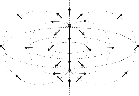
Figure 2: Isovector field configuration around Nambu’ dumb-bell configuration. The thick solid line is the line of zeroes of the Higgs field, dotted lines are lines of magnetic flux. Dashed lines guide the eye on the equatorial plane

The Higgs field in Nambu’s dumb-bell configuration vanishes along a line segment, taking the form away from this line

$$\Phi=\pmatrix{\cos\Theta\cr\sin\Theta e^{i\varphi}\cr}{v\over\sqrt{2}},\qquad\cos 2\Theta=\cos\theta_{+}-\cos\theta_{-}+1,$$ (16)

where $\theta_{\pm}$ are polar angles measured from the ends of the line segment (see Figure 3). The gauge fields can be written in terms of the Higgs field, by solving the equation $D_{i}\Phi=0$:

$$gW_{i}^{a} = -\epsilon^{abc}\hat{\phi}^{b}\partial_{i}\hat{\phi}^{c}-i\cos^{2}\theta_{\rm W}\hat{\phi}^{a}(\hat{\Phi}^{{\dagger}}\vbox{\halign{#\cr$\leftrightarrow$\crcr\kern-1.0pt\nointerlineskip\cr$\hfil\displaystyle{\partial}\hfil$\crcr}}_{i}\hat{\Phi}),$$ (19)

$$g^{\prime}Y_{i} = -i\sin^{2}\theta_{\rm W}(\hat{\Phi}^{{\dagger}}\vbox{\halign{#\cr$\leftrightarrow$\crcr\kern-1.0pt\nointerlineskip\cr$\hfil\displaystyle{\partial}\hfil$\crcr}}_{i}\hat{\Phi}).$$ (22)

This solution actually requires two extra pieces of information: that vortices carry only Z flux (and no electromagnetic flux); and a gauge choice, which sets a possible arbitrary abelian part $(\alpha_{i}\hat{\phi}^{a},\alpha_{i})$ to zero. The second point is a crucial one, for the sphaleron is usually exhibited in the radial gauge, so direct comparisons can be misleading. In Nambu’s paper the fact that a gauge choice has been made is rather implicit: a clearer discussion (for the Georgi-Glashow model) was given by Manton,${}^{\ref{Man77}}$ who showed that in this gauge $\hat{\phi}^{a}$ is constant along lines of magnetic flux, or

$$B^{\rm em}_{i}\partial_{i}\hat{\phi}^{a}=0.$$ (23)

This is illustrated in Figure 2, which depicts the flux lines originating from the ends of the line segment. An important point about this configuration is that away from the singular line the fields obey the equations of motion: that is, not only does the covariant derivative of the Higgs vanish, but also $\epsilon_{ijk}\partial_{j}B^{\rm em}_{k}=0$.

Now, for the purposes of comparison, let us try and construct a sphaleron-type configuration in this gauge, which also vanishes on a line segment. The most convenient way to do this is to use prolate spheroidal coordinates $(\mu,\beta,\varphi)$.${}^{\ref{MorFes53}}$ The surfaces of constant $\mu$ are increasingly prolate as $\mu\to 0$, collapsing to a line of length $2d$ at $\mu=0$, while becoming more spherical as $\mu\to\infty$. $(\beta,\varphi)$ are polar coordinates on the spheroids. If $r_{\pm}$ are the distances from the ends of the line segment then $d\cosh\mu=(r_{+}+r_{-})/2$, and $\cos\beta=(r_{+}-r_{-})/2d$. Then we may adapt (9) by redefining $U$:

$$U(\hat{\mbox{\boldmath$\xi$}})=[\cos\chi(\mu)+i\sin\chi(\mu)\mbox{\boldmath$\sigma$}\cdot\hat{\mbox{\boldmath$\xi$}}]\sigma_{2},$$ (24)

where $\hat{\mbox{\boldmath$\xi$}}=(\sin\beta\cos\varphi,\sin\beta\sin\varphi,\cos\beta)$; and $\chi(0)=\pi/2$, $\chi(\infty)=0$. In the limit that $d\to 0$, $\hat{\mbox{\boldmath$\xi$}}\to\hat{\mbox{\boldmath$x$}}$, and away from the origin the configuration is just a gauge transformation $\Omega=\exp(i(\pi/2-\chi)\mbox{\boldmath$\sigma$}\cdot\hat{\mbox{\boldmath$x$}})$ of the sphaleron. The isovector field can be used to trace the magnetic flux lines:

$$\hat{\phi}^{a}=\cos 2\chi(\delta^{a3}-\hat{\xi}^{a}\hat{\xi}^{3})+\sin 2\chi\epsilon^{a13}\hat{\xi}^{i}+\hat{\xi}^{a}\hat{\xi}^{3}.$$ (25)

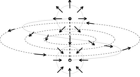
Figure 3: Isovector field configuration around the stretched sphaleron. Only one line of magnetic flux is shown. Note the twist as it travels between the ends of the line of Higgs field zeroes.

Figure 3 shows the isovector field configuration around this “stretched” sphaleron. It is clear that the magnetic field has an azimuthal component: the lines of flux twist through $\pi$ as they travel from one pole to another. This twist is the source of the difference between the sphaleron and the dumb-bell, for it turns out to be crucial in supplying the Chern-Simons number.${}^{\ref{VacFie94}}$ Twisting the field is an unnatural thing to do, for the magnetic field cannot sustain such a twist without a current. The current can only exist in the core of the string segment, where the Higgs field is off the vacuum and $F^{a}_{ij}D_{j}\hat{\phi}^{a}$ does not vanish. Thus, without an external electromagnetic current, the twist can exist only within the string.

The true significance of these field configurations is rather obscure, for they are not solutions of the field equations. However, they may be solutions to the equations subject to a constraint: that the Higgs field is forced to vanish on a line. This is certainly a well-defined variational problem, for the constraint is gauge-invariant. However, to find which (if either) of the dumb-bell or the stretched sphaleron is a solution seems exceedingly hard.

REFERENCES

1. M. Hindmarsh and M. James, Phys. Rev. D, (to appear, 1994).

2. G. ’t Hooft, Nucl. Phys. B79, 276 (1974).

3. Y. Nambu, Nucl. Phys. B130, 505 (1977).

4. T.Vachaspati, “Electroweak Strings: a Progress Report”, in: proceedings of Texas/PASCOS 92: Relativistic Astrophysics and Particle Cosmology, Ann. N. Y. Acad. Sci.  Vol. 688, (1993).

5. M. Barriola, T. Vachaspati and M. Bucher, Embedded Defects, Phys. Rev. D (to appear, 1994).

6. B. Kleihaus, J. Kunz and Y. Brihaye, Phys. Rev. D46, 3587 (1992).

7. F. Klinkhamer and N. Manton, Phys. Rev. D30, 2212 (1984).

8. M. James, Zeit. Phys. C55, 515 (1992).

9. A.M. Polyakov, JETP Lett. 20, 194 (1974).

10. T. Vachaspati, Phys. Rev. Lett. 68, 1977 (1992).

11. M. James, L. Perivolaropoulos and T. Vachaspati, Nucl. Phys. B395, 534 (1993).

12. N. Manton, Nucl. Phys. B126, 525 (1977).

13. P. Morse and H. Feschbach, “Methods of Mathmatical Physics,” McGraw-Hill, New York (1953).

14. T. Vachaspati and G.B. Field, Tufts U. preprint (1994).