Electromagnetic Pion Form Factor
and Neutral Pion Decay Width

Abstract

The electromagnetic pion form factor, $F_{\pi}(q^{2})$, is calculated for spacelike-$q^{2}$ in impulse approximation using a confining quark propagator, $S$, and a dressed quark-photon vertex, $\Gamma_{\mu}$, obtained from realistic, nonperturbative Dyson-Schwinger equation studies. Good agreement with the available data is obtained for $F_{\pi}(q^{2})$ and other pion observables, including the decay $\pi^{0}\rightarrow\gamma\,\gamma$. This calculation suggests that soft, nonperturbative contributions dominate $F_{\pi}(q^{2})$ at presently accessible $q^{2}$.

1 Introduction

As a bound state of a light quark and antiquark, the pion is an ideal system for exploring the application of different approaches to the study of bound state structure in QCD, which is intrinsically nonperturbative. Such studies are constrained by the Goldstone boson nature of the pion. The internal structure of the pion affects its observable properties. The pion electromagnetic form factor, $F_{\pi}(q^{2})$, is one observable that is sensitive to this internal structure and it has been much studied [1, 2, 3].

Perturbative QCD has been employed in order to estimate the behaviour of $F_{\pi}(q^{2})$ at large spacelike-$q^{2}$. These analyses rely on the separation of the amplitude into a product of soft and hard contributions using a factorisation Ansatz [4], however, the applicability of this approach to exclusive processes is uncertain. In this factorisation approach $F_{\pi}(q^{2})$ is the product of a soft contribution that depends on the bound-state Bethe-Salpeter amplitude, which provides only the overall normalisation, and a hard contribution that is independent of the bound-state Bethe-Salpeter amplitude and is taken to be given by the Born amplitude for a collinear quark-antiquark pair, each massless, to scatter coherently from a virtual photon. This analysis yields $q^{2}\,F_{\pi}(q^{2})=16\,\alpha(q^{2})\,f_{\pi}^{2}$ as spacelike-$q^{2}\rightarrow\infty$, where $f_{\pi}\approx 92$ MeV and $\alpha(q^{2})$ is the running coupling constant in QCD.

It is not clear whether presently accessible values of $q^{2}$ are large enough to test predictions based on perturbative analyses in QCD. It is argued in Ref. [5] that they are not; i.e., that the factorisation Ansatz is invalid at presently accessible values of $q^{2}$ and hence that the $q^{2}$ dependence of the quark momentum distribution in the pion provides an important contribution to $F_{\pi}(q^{2})$. This conclusion is supported by Ref. [6] and by the fact that a good fit to the experimental data, over the entire range of available $q^{2}$, is possible using the light-front formulation of a relativistic constituent quark model [1], which has no obvious connection with perturbative QCD.

Herein the impulse approximation to $F_{\pi}(q^{2})$, illustrated in Fig. 1, is calculated for spacelike-$q^{2}$ as a phenomenological application of the nonperturbative Dyson-Schwinger equation [DSE] approach to QCD, which is reviewed in Ref. [7]. The primary elements of this calculation are: 1) The dressed quark propagator, $S(p)$, which is confining in the sense that it has no singularities that can lead to free-quark production thresholds in Fig. 1; i.e., there is no quark mass-shell; 2) The pion Bethe-Salpeter amplitude, $\Gamma_{\pi}(p,P)$, which is regular for spacelike values of $p$, the relative $q-\overline{q}$ momentum. In the chiral limit, $m\to 0$, $\Gamma_{\pi}(p,P)$ is completely determined by the dressed quark propagator, which is a manifestation of Goldstone’s theorem in DSE approach[8]; and 3) The dressed quark-photon vertex, $\Gamma_{\mu}(p_{1},p_{2})$, which is regular in the spacelike region; i.e., away from resonances such as the $\rho$-meson, and follows from extensive QED studies[9, 10, 11]. These properties, which together are sufficient to ensure confinement, entail that this impulse approximation calculation is free of both endpoint and pinch singularities, which arise in perturbative analyses.

Figure 1: A pictorial representation of the amplitude identified with the $\pi$-$\pi$-$A_{\mu}$ vertex in impulse approximation: pions - thick, straight external lines; $\langle\pi|\overline{q}q\rangle$ Bethe-Salpeter amplitudes - filled circles at the $\pi$-legs; photon - wiggly line; dressed quark-photon vertex, which satisfies the Ward-Takahashi Identity, Eq. (24) - shaded circle at the the photon-leg; dressed quarks - thin internal lines.

In phenomenological applications of the DSE approach the model dependence is restricted to spacelike-$q^{2}\mathrel{\hbox to0.0pt{\lower 4.0pt\hbox{\hskip 1.0pt$\sim$}\hss}\raise 1.0pt\hbox{$<$}}2$ GeV², and is realised in a modelling of the form of the quark-quark interaction in the infrared. This not only incorporates information obtained about, for example, the gluon condensate in the QCD sum rules approach [12] but also extends it. The calculation of experimental observables in this approach therefore allows one to place constraints on the qualitative and quantitative features of the effective quark-quark interaction at small spacelike-$q^{2}$ in QCD and to infer the $q^{2}$ scale where perturbative, model-independent, effects begin to dominate.

In Sec. 2 the impulse approximation and its primary elements [$S$, $\Gamma_{\pi}$ and $\Gamma_{\mu}$] are discussed in detail. The width $\Gamma_{\pi^{0}\rightarrow\gamma\gamma}$ is calculated in impulse approximation in Sec. 3 and shown to be independent of the details of $S$, $\Gamma_{\pi}$ and $\Gamma_{\mu}$ in the chiral limit. This illustrates the manner in which anomalies are realised in the present framework. The calculation of $F_{\pi}(q^{2})$ for spacelike-$q^{2}$, and other pion observables, is described in Sec. 4 and the results compared with experiment. The behaviour of $F_{\pi}(q^{2})$ at large spacelike-$q^{2}$ in impulse approximation is determined analytically in Sec. 5: $F_{\pi}(q^{2})\propto 1/q^{4}$, up to $\ln[q^{2}]$-corrections. This result is verified numerically and found to become dominant only for spacelike-$q^{2}\mathrel{\hbox to0.0pt{\lower 4.0pt\hbox{\hskip 1.0pt$\sim$}\hss}\raise 1.0pt\hbox{$>$}}10$ GeV², which is presently inaccessible experimentally. This asymptotic form is a consequence of the realisation of confinement explored herein. Its validity or otherwise is not an essential consequence of the DSE framework. The results are summarised and conclusions presented in Sec. 6.

2 Impulse Approximation

Herein all calculations are carried out in Euclidean space, with $\gamma_{\mu}$ hermitian and metric $\delta_{\mu\nu}={\rm diag}(1,1,1,1)$.

One may define the impulse approximation to the connected $\pi$-$\pi$-$A_{\mu}$ vertex in QCD as, with $m_{u}=m_{d}$,

$$\Lambda_{\mu}(P+q,-P)=\frac{2N_{c}}{f_{\pi}^{2}}\,\int\mbox{\footnotesize$\frac{d^{4}k}{(2\pi)^{4}}$}\,{\rm tr}_{D}\left[\overline{\Gamma}_{\pi}(k;P+q)\times\right.$$

$$\left.S(k_{++})i\Gamma_{\mu}(k_{++},k_{-+})S(k_{-+})\Gamma_{\pi}(k-\mbox{\footnotesize$\frac{1}{2}$}q;-P)S(k_{--})\right]~{},$$

where $q$ is the photon momentum and $P$ is the initial momentum of the pion. Here the trace over colour and flavour indices has been evaluated leaving only the trace over Dirac indices and

$$k_{\alpha\beta}=k+\mbox{\footnotesize$\frac{\alpha}{2}$}q+\mbox{\footnotesize$\frac{\beta}{2}$}P~{}.$$ (2)

In Eq. (2): $\Gamma_{\mu}(p_{1},p_{2})$ denotes the dressed quark-photon vertex; $\Gamma_{\pi}(p;P)$ the pion Bethe-Salpeter amplitude, with $p$ the relative momentum and $P$ the centre-of-mass momentum; and $S(p)$ the dressed quark propagator. The Bethe-Salpeter wave-function is

$$\chi_{\pi}(p;P)=S(p+\mbox{\footnotesize$\frac{1}{2}$}P)\,\Gamma_{\pi}(p;P)\,S(p-\mbox{\footnotesize$\frac{1}{2}$}P)~{}.$$ (3)

The impulse approximation, Eq. (2), is illustrated in Fig. 1 and can be derived as an application of the formalism described in Ref. [13]. Its definition is only complete when the functions $S$, $\Gamma_{\pi}$ and $\Gamma_{\mu}$ have been fully specified, which is the subject of Secs. 2.1, 2.2 and 2.3, respectively.

2.1 Quark Propagator

The dressed quark propagator in Eq. (2) can be obtained by solving the following Dyson-Schwinger equation [DSE]:

$$S^{-1}(p)=i\gamma\cdot p+m+\mbox{\footnotesize$\frac{4}{3}$}g^{2}\int\mbox{\footnotesize$\frac{d^{4}k}{(2\pi)^{4}}$}\gamma_{\mu}S(k)\Gamma_{\nu}^{g}(k,p)D_{\mu\nu}(p-k),$$ (4)

where $m=(m_{u}+m_{d})/2$ is the current-quark mass. Here $D_{\mu\nu}(k)$ is the dressed gluon propagator and $\Gamma_{\mu}^{g}(p_{1},p_{2})$ is the dressed quark-gluon vertex; each of which satisfies its own DSE. The general form of the solution of Eq. (4) is

$$S(p)=-i\gamma\cdot p\,\sigma_{V}(p^{2})+\sigma_{S}(p^{2}),$$ (5)

which can also be written as

$$S(p)=\frac{1}{i\gamma\cdot p\,A(p^{2})+m+B(p^{2})}~{}.$$ (6)

This equation has been much studied and the general properties of $\sigma_{S}$ and $\sigma_{V}$ in QCD are well known [7].

As a simple example, in Ref. [14] Eq. (4) was solved with

$$g^{2}D_{\mu\nu}(k)=\left(\delta_{\mu\nu}-\frac{k_{\mu}k_{\nu}}{k^{2}}\right)8\pi^{4}D\delta^{4}(k)\;\; \;\;\Gamma_{\mu}(p,p)=-i\partial_{\mu}S^{-1}(p)~{},$$ and (7)

where $D$ is a mass-scale parameter. This Ansatz for the dressed gluon propagator models the infrared behaviour of the quark-quark interaction in QCD via an integrable infrared singularity, as suggested by Refs. [15, 16, 17], and and is sufficient to ensure confinement, in the sense described below. The Ansatz for the dressed-quark gluon vertex is the result of extensive analysis of its general form [9, 10, 11]. The solution of Eq. (4) in Ref. [14] is

$$\bar{\sigma}_{S}(y)=$$

$$\frac{C}{2\overline{m}y}\exp(-2y^{2})J_{1}(4\bar{m}y)+\frac{\overline{m}^{2}}{y}\int_{0}^{\infty}\,d\xi\,\xi\,K_{1}(\bar{m}\xi)\,J_{1}(y\xi)\exp\left(-\frac{\xi^{2}}{8}\right)~{},$$

with $\overline{m}=m/\sqrt{2D}$, $y^{2}=p^{2}/(2D)$ and where $J_{1}$ and $K_{1}$ are Bessel functions, and

$$\bar{\sigma}_{V}(y)=\frac{1}{\bar{m}}\left(\bar{\sigma}_{S}(y)+\frac{1}{4y}\frac{d}{dy}\bar{\sigma}_{S}(y)\right)~{},$$ (9)

with $\bar{\sigma}_{S}(y^{2})=\sqrt{2\,D}\,\sigma_{S}(k^{2})$ and $\bar{\sigma}_{V}(y^{2})=2\,D\,\sigma_{V}(k^{2})$. In Eq. (2.1), $C$ is a parameter associated with dynamical chiral symmetry breaking and it is not determined by Eq. (4) with Eq. (7), while the integral, which is associated with explicit chiral symmetry breaking, cannot be evaluated in terms of known functions.

At large spacelike-$p^{2}$ one finds from Eqs. (2.1) and (9) that

$$\sigma_{S}(p^{2})\approx\frac{m}{p^{2}}-\frac{m^{3}}{p^{4}}+\ldots\;\; \;\;\sigma_{V}(p^{2})\approx\frac{1}{p^{2}}-\frac{D+m^{2}}{p^{4}}+\ldots~{}.$$ and (10)

At large spacelike-$p^{2}$ in QCD one has at leading order

$$\sigma_{S}(p^{2})\approx\frac{\hat{m}}{p^{2}\left[\mbox{\footnotesize$\frac{1}{2}$}\ln\left(p^{2}/\Lambda_{\rm QCD}^{2}\right)\right]^{d}}$$ (11)

with $\hat{m}$ a renormalisation point invariant and $d=12/[33-2N_{f}]$; $N_{f}$ is the number of quark flavours. One therefore sees that, neglecting $\ln[p^{2}]$ terms, the model defined by Eqs. (4) and (7) incorporates asymptotic freedom.

Another feature of this model is that both $\sigma_{S}$ and $\sigma_{V}$ are entire functions in the complex-$p^{2}$ plane with an essential singularity. As a consequence the quark propagator does not have a Lehmann representation and can be interpreted as describing a confined particle. This is because, when used in Eq. (2), for example, this property ensures the absence of free-quark production thresholds, under the reasonable assumptions that $\Gamma_{\pi}$ is regular for spacelike-$p^{2}$ and $\Gamma_{\mu}$ is regular for spacelike-$q^{2}$. It follows from this that Eq. (2) is free of endpoint and pinch singularities.

This is a particular, sufficient manner in which to realise the requirement that Fig. 2 have no free-quark production thresholds, which is the definition of confinement explored herein. There are other, more complicated, means of realising this definition but the effect is the same [7]. Some of the phenomenological implications of a model with a simple realisation of this confinement mechanism have been discussed in Ref. [18].

The solution described by Eqs. (2.1) and (9) has a defect. To see this one sets $\bar{m}=0$ in Eq. (2.1), which yields

$$\sigma_{S}(y)=Ce^{-2y^{2}}~{}.$$ (12)

This poorly represents $\sigma_{S}$ for sufficiently large $y$ since, in the absence of a bare mass and when chiral symmetry is dynamically broken, it is known [19] that

$$\left.\sigma_{S}(y)\right|_{y\rightarrow\infty}\rightarrow\,\frac{4\pi^{2}d}{3}\frac{\kappa}{y^{2}\,(\ln\,y^{2})^{1-d}}$$ (13)

with $\kappa=\,-\,(\ln[\mu^{2}/\Lambda_{QCD}^{2}])^{-d}\,\langle\bar{q}q\rangle_{\mu^{2}}$, a renormalisation point invariant. This defect results from the fact that, although the form of $D_{\mu\nu}(k)$ in Eq. (7) generates confinement, it underestimates the strength of the coupling in QCD for sufficiently large $k^{2}$. In the numerical studies of Eq. (4) that have used a better approximation to $D_{\mu\nu}(k)$ [20] there is no such defect.

2.1.1 Approximate, algebraic quark propagator

Herein, to avoid the need for a numerical solution of Eq. (4), Eqs. (2.1) and (9) are simply modified so as to restore the missing strength at intermediate-$x\,(=y^{2})$ and thereby provide a better approximation to the realistic numerical solutions [20], while retaining the confining characteristics present in the model example described in association with Eqs. (2.1) and (9).

The following approximating algebraic forms are used:

$$\bar{\sigma}_{S}(x)=Ce^{-2x}+$$

$$\frac{1-e^{-b_{1}x}}{b_{1}x}\,\frac{1-e^{-b_{3}x}}{b_{3}x}\,\left(b_{0}+b_{2}\frac{1-e^{-\Lambda x}}{\Lambda\,x}\right)+\frac{\bar{m}}{x+\bar{m}^{2}}\left(1-e^{-2\,(x+\bar{m}^{2})}\right)~{},$$

$$\bar{\sigma}_{V}(x) = \frac{2(x+\bar{m}^{2})-1+e^{-2(x+\bar{m}^{2})}}{2(x+\bar{m}^{2})^{2}}-\bar{m}Ce^{-2x},$$ (15)

which are entire functions, as in the model described above, and allow the propagator to be consistent with realistic numerical solutions of Eq. (4).

When $b_{0}=0=b_{2}$, Eqs. (2.1.1) and (15) provide an excellent approximation to Eqs. (2.1) and (9) [21], while for nonzero values of these parameters it is clear that the behaviour given in Eq. (13) is recovered, up to $\ln[p^{2}]$-corrections. These model forms are also entire functions in the complex $p^{2}$ plane with an essential singularity.

The expressions in Eqs. (2.1.1) and (15) provide a six parameter model of the quark propagator in QCD: $C$, $\bar{m}$, $b_{0},\ldots,b_{3}$. [$\Lambda(=10^{-4})$ is introduced simply to decouple $b_{2}$ from the quark condensate, as will be shown below.] These parameters can be fitted to experimental observables and Eq. (4) used to place constraints on $D_{\mu\nu}(k)$, the effective gluon propagator. In $S$ one therefore has an implicit parametrisation of $D_{\mu\nu}(k)$ and hence a connection between experimental observables and the nature of the effective quark-quark interaction in the infrared. A phenomenologically successful application of this procedure may then make possible the use of precise experimental data as a probe of the effective quark-quark interaction in the infrared.

2.2 Pion Bethe-Salpeter Amplitude

The Bethe-Salpeter amplitude in Eq. (2) is the solution of the homogeneous Bethe-Salpeter equation [BSE]:

$$\Gamma^{rs}_{\pi}(p;P)=\int\,\mbox{\footnotesize$\frac{d^{4}k}{(2\pi)^{4}}$}\,K^{rs;tu}(k,p;P)\,\left(S(k+\mbox{\footnotesize$\frac{1}{2}$}P)\Gamma_{\pi}(k;P)S(k-\mbox{\footnotesize$\frac{1}{2}$}P)\right)^{tu}$$ (16)

where $P$ is the centre-of-mass momentum of the bound state, $p$ is the relative momentum between the quarks in the bound state and the superscripts are associated with the Dirac structure of the amplitude. In the isospin symmetric case, $m_{u}=m_{d}$, $K^{rs;tu}(p,k;P)\propto I_{F}$, the identity matrix in flavour-space. Further, since $\Gamma_{\pi}$ and $S(p)$ are $\propto I_{C}$, the identity matrix in colour-space, then $K^{rs;tu}(p,k;P)\propto I_{C}$ also.

The generalised-ladder approximation is defined by the choice

$$K^{rs;tu}(p,k;P)=\mbox{\footnotesize$\frac{4}{3}$}\,g^{2}D_{\mu\nu}(p-k)\,(\gamma_{\mu})^{rt}\,(\gamma_{\nu})^{us}$$ (17)

in Eq. (16), with $D_{\mu\nu}(p-k)$ the dressed gluon propagator and $S(p)$ the dressed quark propagator obtained from Eq. (4). This equation has been much studied [22]. In using dressed quark and gluon propagators, the generalised-ladder approximation is a significant advance over the ladder approximation familiar in QED where perturbative fermion and photon propagators are used. The amplitude obtained as a solution in generalised-ladder approximation defines the nonperturbative “dressed-quark core” of the meson and provides the dominant contribution to physical observables, as will be seen herein.

The most general form of $\Gamma_{\pi}$ allowed by Lorentz covariance, which is odd under parity transformations, is [23]

$$\Gamma_{\pi}(p;P)=i\gamma_{5}\left\{\rule{0.0pt}{17.07164pt}\,E(p;P)+\right.$$

$$\left.\rule{0.0pt}{17.07164pt}\ i\gamma\cdot p\,p\cdot P\,F(p;P)+i\gamma\cdot P\,G(p;P)+[\gamma\cdot p,\gamma\cdot P]\,H(p;P)\right\}$$

where, since $\pi^{0}$ is even under charge-conjugation, $E$, $F$, $G$ and $H$ are even functions of $(p\cdot P)$. The many studies of Eq. (16) using Eq. (17) [22] suggest that the dominant amplitude in Eq. (2.2) is $E(p;P)$, with the other functions providing $\sim$ 10% contribution to physical observables; i.e., that it is a good approximation to write

$$\Gamma_{\pi}(p,P)=i\gamma_{5}\,E(p;P)~{}.$$ (19)

In generalised-ladder approximation $K$ is independent of $P$ and the standard normalisation condition for $\Gamma_{\pi}$ reduces to the requirement that, for $P^{2}=-m_{\pi}^{2}$:

$$P_{\mu} = N_{c}\,\int\,\mbox{\footnotesize$\frac{d^{4}k}{(2\pi)^{4}}$}\,{\rm tr}_{D}\left[\overline{\Gamma}_{\pi}(k;P)\frac{\partial S(k_{0+})}{\partial P_{\mu}}\Gamma_{\pi}(k;-P)S(k_{0-})\;+\right.$$

$$\left.\overline{\Gamma}_{\pi}(k;P)S(k_{0+})\Gamma_{\pi}(k;-P)\frac{\partial S(k_{0-})}{\partial P_{\mu}}\right]~{}.$$

2.2.1 Pion as Goldstone mode and quark-antiquark bound state

In the chiral limit; i.e., when the current quark mass, $m$, is zero, the pseudoscalar generalised-ladder approximation BSE and quark rainbow-DSE [which has $\Gamma^{g}_{\mu}=\gamma_{\mu}$ in Eq. (4)] are identical [8]. This entails that there is a massless excitation in the pseudoscalar channel with

$$E(p;P^{2}=0)=\frac{1}{f_{\pi}}\,B_{m=0}(p^{2})~{},$$ (21)

where $B(p^{2})$ is given in Eq. (6) and $f_{\pi}$ is the calculated normalisation constant. This is the manner in which Goldstone’s theorem is realised in the Dyson-Schwinger equation framework. In this case, Eqs. (2.1.1) and (15) completely determine $\Gamma_{\pi}$.

The dichotomy of the pion as both a Goldstone boson and a quark-antiquark bound state is thus easily understood in the DSE approach. One has dynamical chiral symmetry breaking when, with $m=0$, Eq. (4) yields a solution $B_{m=0}(p^{2})\not\equiv 0$; i.e., when a momentum-dependent quark mass is generated dynamically by the interaction of the quark with its own gluon field. For $m=0$ one also finds that the Bethe-Salpeter equation in the pseudoscalar channel reduces to the quark DSE as $P^{2}\to 0$, where $P_{\mu}$ is the total-momentum of the bound state. It therefore follows, without fine tuning, that if the quark-quark interaction is strong enough to support dynamical chiral symmetry breaking then one has a massless, pseudoscalar bound state of a strongly dressed quark and antiquark whose Bethe-Salpeter amplitude is the quark mass function, Eq. (21); i.e., one has a zero mass bound state of a quark and antiquark, each of which has an effective mass of $\sim 200$-$400$ MeV. (The actual value depends on the definition and the strength of the interaction.)

For $m\neq 0$, the pion Bethe-Salpeter amplitude must still vanish as the relative momentum $p^{2}\rightarrow\infty$ [24]. A first, simple approximation in this case is

$$E(p;P^{2}=-m_{\pi}^{2})\approx\frac{1}{f_{\pi}}\,B_{m\neq 0}(p^{2})~{},$$ (22)

which, for small current-quark mass, is very good both pointwise and in terms of the values obtained for physical observables [25]. One notes that using Eqs. (2.1.1) and (15) in Eq. (22) entails

$$\Gamma_{\pi}(p,P)\propto\frac{1}{p^{2}},$$ (23)

which, up to the $\ln[p^{2}]$-corrections associated with the anomalous dimension, reproduces the ultraviolet behaviour of the Bethe-Salpeter amplitude given by QCD [24].

2.3 Quark-photon Vertex

The quark-photon vertex, $\Gamma_{\mu}(p_{1},p_{2})$, satisfies a DSE that describes both strong and electromagnetic dressing of the interaction. Solving this equation is a difficult problem that has recently begun to be addressed [26]. Much progress has been made in constraining the form of $\Gamma_{\mu}(p_{1},p_{2})$ and developing a realistic Ansatz [10, 11].

The bare vertex: $\Gamma_{\mu}(p_{1},p_{2})=\gamma_{\mu}$, is inadequate when the fermion propagator has momentum dependent dressing because it violates the Ward-Takahashi identity:

$$(p_{1}-p_{2})_{\mu}i\gamma_{\mu}\neq S^{-1}(p_{1})-S^{-1}(p_{2})~{};$$ (24)

and hence leads to an electromagnetic current for the pion that is not conserved.

An Ansatz [10] fulfilling the criteria [11] that it a) satisfies the Ward-Takahashi identity; b) is free of kinematic singularities; c) reduces to the bare vertex in the free field limit as prescribed by perturbation theory; and d) has the same transformation properties as the bare vertex under charge conjugation and Lorentz transformations, is

$$\Gamma_{\mu}(p,k)=\Gamma_{\mu}^{\rm BC}(p,k)+\Gamma_{\mu}^{\rm T}(p,k)$$ (25)

where [9]

$$\Gamma_{\mu}^{\rm BC}(p,k)=\frac{\left[A(p^{2})+A(k^{2})\right]}{2}\;\gamma_{\mu}+$$

$$\frac{(p+k)_{\mu}}{p^{2}-k^{2}}\left\{\left[A(p^{2})-A(k^{2})\right]\frac{\left[\gamma\cdot p+\gamma\cdot k\right]}{2}-i\left[B(p^{2})-B(k^{2})\right]\right\}$$

and $(p-k)_{\mu}\,\Gamma_{\mu}^{\rm T}(p,k)=0$ with $\Gamma_{\mu}^{\rm T}(p,p)=0$. $\Gamma_{\mu}^{\rm BC}$ in Eq. (25) is completely determined by the dressed quark propagator but $\Gamma_{\mu}^{\rm T}$ must be determined otherwise. Gauge covariance of the fermion propagator and multiplicative renormalisability of the fermion DSE can be used [10, 11] to place constraints on $\Gamma_{\mu}^{\rm T}(p,k)$. Using the bare quark propagator, which has $A=1$ and $B=$ constant, $\Gamma_{\mu}^{\rm T}=0$.

The definition of the impulse approximation is complete with

$$\Gamma_{\mu}(p,k)\approx\Gamma_{\mu}^{\rm BC}(p,k)~{}$$ (27)

in Eq. (2).

2.3.1 Vector meson dominance

The electromagnetic pion form factor, $F_{\pi}(q^{2})$, is an analytic function but for a cut extending from $q^{2}=-\infty$ to $-4m_{\pi}^{2}$; i.e., on the timelike real axis. It is real for $q^{2}>-4m_{\pi}^{2}$. Generalised vector meson dominance is the observation that the pion form factor is completely determined by the spectral density associated with the $J^{PC}=1^{--}$ pion-photon vertex, which is the discontinuity across this cut.

Models of vector meson dominance consist in a phenomenological Ansatz for this spectral density. A common model is a single, $\rho$-meson pole representation. Since the vertex in Equation (27) is free of kinematic singularities, by construction in accordance with criterion b) above, vector meson pole contributions of this type are explicitly excluded in impulse approximation.

Explicit vector-meson–photon mixing contributions to $F_{\pi}(q^{2})$ enter through the dressed quark-photon vertex and only appear in $\Gamma_{\mu}^{\rm T}(p,k)$ because vector mesons are resonances, which are only uniquely defined on shell where they are transverse. They appear via resonance contributions in the timelike region to the hadronic component of the photon vacuum polarisation.

For $q^{2}=0$ the differential form of the Ward identity, $\Gamma_{\mu}(p,p)=-i\partial_{\mu}S(p)$, completely determines the quark-photon vertex ($\Gamma_{\mu}^{\rm T}(p,p)=0$). This entails that the pion charge radius is primarily determined by the dressed quark propagator and is not very sensitive to $\Gamma_{\mu}^{\rm T}(p,k)$. In the sense of generalised vector meson dominance described above, this admits an interpretation that the charge radius is primarily determined by the non-resonant part of the full spectral density near threshold. To go further and identify this as the “tail of the $\rho$-meson resonance” involves additional model assumptions since the vector mesons are resonances, whose definition off-shell is arbitrary.

This point is also discussed in Ref. [27].

2.4 Current Conservation

Using Eq. (27) and the identities:

$$\begin{array}[]{ll}S(-k)^{T}=C^{\dagger}\,S(k)\,C;&\Gamma_{\pi}^{T}(-k;p)=C^{\dagger}\,\Gamma_{\pi}(k;p)\,C;\\ \bar{\Gamma}_{\pi}^{T}(-k;p)=C^{\dagger}\,\bar{\Gamma}_{\pi}(k;p)\,C;&\Gamma_{\mu}^{T}(-k,-p)=-C^{\dagger}\,\Gamma_{\mu}(p,k)\,C,\end{array}$$ (28)

where $C=\gamma_{2}\gamma_{4}$ is the charge conjugation matrix, one finds easily that the $\pi$-current is conserved:

$$q_{\mu}\Lambda_{\mu}(P+q,-P)=0~{}.$$ (29)

For elastic scattering, with $[2q\cdot P+q^{2}=0]$, one can therefore write

$$\Lambda_{\mu}(P+q,-P)=\left(2P+q\right)_{\mu}F_{\pi}(q^{2},P^{2})~{}.$$ (30)

One obtains similarly that

$$\Lambda_{\mu}(P,-P)=2P_{\mu}\,F_{\pi}(0,P^{2})=2N_{c}\int\mbox{\footnotesize$\frac{d^{4}k}{(2\pi)^{4}}$}{\rm tr}_{D}\left[\overline{\Gamma}_{\pi}(k;P)\frac{\partial S(k_{0+})}{\partial P_{\mu}}\times\right.$$

$$\left.\Gamma_{\pi}(k;-P)S(k_{0-})+\overline{\Gamma}_{\pi}(k;P)S(k_{0+})\Gamma_{\pi}(k;-P)\frac{\partial S(k_{0-})}{\partial P_{\mu}}\right]~{}.$$

Comparing this with Eq. (2.2) it is clear that in impulse approximation $F_{\pi}(0,P^{2})=1$ only if the Bethe-Salpeter kernel is independent of $P$; i.e., impulse approximation combined with a $P$-independent Bethe-Salpeter kernel provides a consistent approximation scheme. In this case one has, in the chiral limit $P^{2}=-m_{\pi}^{2}=0$:

$$f_{\pi}^{2}=\frac{N_{c}}{8\pi^{2}}\int_{0}^{\infty}\,ds\,s\,B(s)^{2}\,$$

$$\left(\sigma_{V}^{2}-2\left[\sigma_{S}\sigma_{S}^{\prime}+s\sigma_{V}\sigma_{V}^{\prime}\right]-s\left[\sigma_{S}\sigma_{S}^{\prime\prime}-\left(\sigma_{S}^{\prime}\right)^{2}\right]-s^{2}\left[\sigma_{V}\sigma_{V}^{\prime\prime}-\left(\sigma_{V}^{\prime}\right)^{2}\right]\right)~{},$$

with $s=p^{2}$.

This shows that the impulse approximation to the form factor, Eq. (2), is regular in the chiral limit. In fact, the calculated results are only weakly dependent on $m_{\pi}$. The study of Ref. [27] indicates that, at $m_{\pi}=0.14$ GeV, Eq. (2) provides the dominant contribution to $F_{\pi}(q^{2})$ for spacelike-$q^{2}$ and that pion-loops are unimportant.

3 Neutral pion decay

In Euclidean space the matrix element for the decay $\pi^{0}\rightarrow\gamma\gamma$ can be written

$${\cal M}(k_{1},k_{2})=-2\,i\,\frac{\alpha_{em}}{\pi f_{\pi}}\,\epsilon_{\mu\nu\rho\sigma}\epsilon_{\mu}(k_{1})\,\epsilon_{\nu}(k_{2})\,k_{1\rho}\,k_{2\sigma}\,G(k_{1}\cdot k_{2})~{},$$ (33)

where $k_{i}$ are the photon momenta and $\epsilon(k_{i})$ are their polarisation vectors. Here, the $\pi^{0}$ momentum is $P=(k_{1}+k_{2})$ and $P^{2}=2\,k_{1}\cdot k_{2}$.

Using Eq. (33) one finds easily that

$$\Gamma_{\pi^{0}\rightarrow\gamma\gamma}=\frac{m_{\pi}^{3}}{16\pi}\,\left(\frac{\alpha_{em}}{\pi f_{\pi}}\right)^{2}G(-m_{\pi}^{2})^{2}~{}.$$ (34)

Experimentally one has $\Gamma_{\pi^{0}\rightarrow\gamma\gamma}=(7.74\pm 0.56)~{}\mbox{eV}$, which corresponds to

$$g_{\pi^{0}\gamma\gamma}\equiv G(-m_{\pi}^{2})=0.500\pm 0.018~{},$$ (35)

using $m_{\pi^{0}}=135$ MeV and $f_{\pi}=92.4$ MeV.

In impulse approximation one has

$$i\frac{\alpha_{em}}{\pi f_{\pi}}\,\epsilon_{\mu\nu\rho\sigma}\,k_{1\rho}\,k_{2\sigma}\,G(k_{1}\cdot k_{2})=\mbox{\footnotesize$\frac{1}{4\pi^{2}}$}\,\int\,d^{4}k\,{\rm tr}_{D}\left[\rule{0.0pt}{14.22636pt}S(k)\,\right.$$

$$\left.\rule{0.0pt}{14.22636pt}i\Gamma_{\mu}(k,k-k_{1})\,S(k-k_{1})\,\Gamma_{\pi}(k+k_{2}/2;P)\,S(k+k_{2})\,i\Gamma_{\nu}(k+k_{2},k)\,\right]~{}.$$

In the chiral limit, $P^{2}=0$, and using Eq. (19), one easily obtains

$$g_{\pi^{0}\gamma\gamma}^{0}\equiv G(0)=\int_{0}^{\infty}\,ds\,s\,[f_{\pi}\,E(s;0)]\,A\,\sigma_{V}\,\times$$

$$\left\{\rule{0.0pt}{14.22636pt}A\,\left[\sigma_{V}\,\sigma_{S}+s\left(\sigma_{V}^{\prime}\,\sigma_{S}-\sigma_{V}\,\sigma_{S}^{\prime}\right)\right]+s\,\sigma_{V}\,\left(A^{\prime}\,\sigma_{S}-B^{\prime}\sigma_{V}\right)\right\}~{}.$$

Now, defining

$$C(s)=\frac{B(s)^{2}}{s\,A(s)^{2}}=\frac{\sigma_{S}(s)^{2}}{s\,\sigma_{V}(s)^{2}}$$ (38)

one obtains a dramatic simplification and Eq. (3) becomes

$$g_{\pi^{0}\gamma\gamma}^{0}=-\,\int_{0}^{\infty}\,ds\,\frac{f_{\pi}\,E(s;0)}{B(s)}\,\frac{C^{\prime}(s)}{[1+C(s)]^{3}}~{}.$$ (39)

It therefore follows from the manner in which dynamical chiral symmetry breaking is realised in the Dyson-Schwinger equation framework; i.e., from Eq. (21), that in the chiral limit

$$g_{\pi^{0}\gamma\gamma}^{0}=\int_{0}^{\infty}\,dC\,\frac{1}{(1+C)^{3}}=\frac{1}{2}~{},$$ (40)

since $C(s=0)=\infty$ and $C(s=\infty)=0$. Hence, the experimental value is reproduced independent of the details of $S(p)$.

This illustrates the manner in which the Abelian anomaly is incorporated in the Dyson-Schwinger equation framework. Similar results are obtained for the Wess-Zumino five-pseudoscalar term [28] and $\gamma\pi\pi\pi$ interaction [29].

In order to obtain the result in Eq. (40) it is essential that, in addition to Eq. (21), the photon-quark vertex satisfy the Ward identity. This is not surprising. However, the fact that one must dress all of the elements in a calculation consistently is often overlooked.

The subtle cancellations that are required to obtain this result also make it clear that it cannot be obtained in model calculations where an arbitrary cutoff function (or “form-factor”) is introduced into each integral. The fact that $E(p;P^{2}=0)$ is the pion Bethe-Salpeter amplitude and $f_{\pi}\,E(p;P^{2}=0)=B(p^{2})$ in the chiral limit, is crucial.

A good approximation to $g_{\pi^{0}\gamma\gamma}$ for nonzero pion mass is given by Eq. (3) with Eq. (22).

4 Calculated Spacelike Form Factor

The impulse approximation to $F_{\pi}(q^{2})$ is defined by Eq. (2) with the dressed quark propagator obtained from Eq. (4), the Bethe-Salpeter amplitude obtained using Eqs. (16), (17) and the dressed quark-photon vertex in Eq. (27).

If, at large spacelike-$q^{2}$, each of the elements in Eq. (2) behaves as prescribed by the renormalisation group in QCD then this amplitude reduces to that studied in perturbative analyses of the elastic form factor. [To see that the “hard-scattering” contribution is included one need only once-iterate the $\pi$-$q$-$\overline{q}$ vertices using Eq. (16).] It is therefore plausible that a model such as the one described by Eqs. (2.1.1), (15) and (22), constructed so as to preserve this asymptotic behaviour, should provide a result for the large spacelike-$q^{2}$ behaviour of $F_{\pi}(q^{2})$ whose only model dependence is in the confinement mechanism.

Such a model will provide an extrapolation to small spacelike-$q^{2}$ that is sensitive to the model parameters. The DSE framework provides an interpretation of these model parameters in terms of qualitative and quantitative features of the quark-quark interaction in the infrared.

To evaluate Eq. (2) it is convenient to work in the Breit frame with

$$q=(0,0,-q,0) \;\;{\rm and}\;\; P=(0,0,\mbox{\footnotesize$\frac{1}{2}$}q,i\sqrt{m_{\pi}^{2}+\mbox{\footnotesize$\frac{1}{4}$}q^{2}}\,)$$ (41)

in which case, with $k=k\,(\sin\beta\,\sin\theta\,\cos\phi,\sin\beta\,\sin\theta\,\sin\phi,\sin\beta\,\cos\theta,\cos\beta)$,

$$k\cdot q = -k\,q\,\sin\beta\,\cos\theta\,$$ (42)

$$k\cdot P = \mbox{\footnotesize$\frac{1}{2}$}k\,q\sin\beta\,\cos\theta+ik\sqrt{m_{\pi}^{2}+\mbox{\footnotesize$\frac{1}{4}$}q^{2}}\,\cos\beta$$ (43)

and one is left with three integrals to evaluate, one radial and two angular.

The definition of confinement employed herein ensures that, for all spacelike-$q^{2}$, the integrand is regular and hence that the integrals can be evaluated using straightforward Gaussian quadrature techniques; i.e., there are no endpoint or pinch singularities.

4.1 Fitting the Parameters

Equations (2.1.1), (15) and (22) provide a six parameter model [$C$, $\overline{m}$, $b_{0}\ldots b_{3}$] of the nonperturbative dressed-quark substructure of the pion based on DSE studies. These parameters are fixed herein by requiring that the model reproduce, as well as possible, the following experimental values of the dimensionless quantities:

$$\begin{array}[]{ccc}\displaystyle\frac{f_{\pi}}{\langle\overline{q}q\rangle^{\frac{1}{3}}}=0.423~{},&\;\;f_{\pi}\,r_{\pi}=0.318~{},\;\;\displaystyle\frac{m_{\pi}^{2}}{\langle\overline{q}q\rangle^{\frac{2}{3}}}=0.396~{};\end{array}$$ (44)

the dimensionless $\pi$-$\pi$ scattering lengths (see Refs. [30, 31] for a discussion):

$$\begin{array}[]{cc}a_{0}^{0}=0.26\pm 0.05~{},&a_{0}^{2}=-0.028\pm 0.012~{},\\ a_{1}^{1}=0.038\pm 0.002~{},&a_{2}^{0}=0.0017\pm 0.0003~{};\end{array}$$ (45)

and a least-squares fit to $F_{\pi}(q^{2})$ on the spacelike-$q^{2}$ domain: $[0,4]$ GeV². The fitting procedure was performed using the expression for the pion decay constant, $f_{\pi}$, given in Eq. (2.4),

$$\langle\overline{q}q\rangle_{\mu^{2}}=$$

$$\,-\,\left(\ln\frac{\mu^{2}}{\Lambda_{QCD}^{2}}\right)^{\alpha}\lim_{\Lambda_{UV}^{2}\rightarrow\infty}\left(\ln\frac{\Lambda_{UV}^{2}}{\Lambda_{QCD}^{2}}\right)^{-\alpha}\frac{3}{4\pi^{2}}\int_{0}^{\Lambda_{UV}^{2}}\,ds\,s\left(\sigma_{S}(s)-\frac{m}{s+m^{2}}\right)~{},$$

$s=p^{2}$ and $\Lambda_{QCD}=0.20$ GeV, following Ref. [20] but with $\alpha=1$ rather than the anomalous dimension, $d$, because the associated $\ln[p^{2}]$-corrections have not been included in Eqs. (2.1.1) and (15), and the expressions for $a_{0}^{0}$, $a_{0}^{2}$, $a_{1}^{1}$, $a_{2}^{0}$ and $r_{\pi}$ given in Ref. [30]. Using Eq. (2.1.1) in Eq. (4.1) one obtains

$$\langle\overline{q}q\rangle_{\mu^{2}}=\,-\,(2\,D)^{\frac{3}{2}}\,\left(\ln\frac{\mu^{2}}{\Lambda_{QCD}^{2}}\right)\,\frac{3}{4\pi^{2}}\,\frac{b_{0}}{b_{1}\,b_{3}}~{},$$ (47)

which is independent of $b_{2}$ for arbitrarily small but nonzero $\Lambda$.

Following this procedure one obtains

$$\begin{array}[]{cc}C=0.0422~{},&\overline{m}=0.0111~{},\end{array}$$ (49)

$$\begin{array}[]{cccc}b_{0}=0.135~{},&b_{1}=2.48~{},&b_{2}=0.502~{},&b_{3}=0.168~{}.\end{array}$$ (51)

The mass scale is set by requiring equality between the percentage error in $f_{\pi}$ and $r_{\pi}$, which yields $D=0.132$ GeV².

The results obtained are robust in the sense that they are not sensitive to the functional form of the quark propagator. Different functional forms, provided they ensure confinement in the manner described herein, whose parameters are allowed to vary in order to provide a good fit to pion observables, yield a numerical form for the quark propagator that is, pointwise, approximately the same on the integration domain explored by pion observables. Since the quark propagator implicitly constrains the gluon propagator via Eq. (4), the robust nature of the study makes it plausible that pion observables can be used to constrain the dressed-gluon propagator.

To make the connection with the gluon propagator explicit is computationally more intensive, with a calculation of the pion form factor requiring a solution of Eq. (4) off the real-spacelike axis. A first step in that direction is made in Ref. [25], in which a one-parameter model dressed gluon propagator is employed in the calculation of all the observables considered herein, except for the form factor. That study illustrates that all of the parameters in the quark propagator are correlated via the single parameter in the gluon propagator and that one can fit the available pion data to the same level of agreement with only one parameter, in addition to the current quark mass. The quark propagator determined by this gluon propagator agreed well in form and magnitude with the parametrisation employed herein evaluated with the best-fit parameters.

4.2 Results for $F_{\pi}(q^{2})$ and Other Observables.

In Table 1 the low-energy physical observables calculated with the parameter set of Eq. (51) are compared with their experimental values. In this table $m^{\rm ave}=\left(m_{u}+m_{d}\right)/2$ and $m_{\pi}$ is obtained from: $m_{\pi}^{2}\,f_{\pi}^{2}=-\,2\,m^{\rm ave}_{\mu^{2}}\,\langle\bar{q}q\rangle_{\mu^{2}}$. Each of the calculated quantities tabulated here was evaluated at the listed value of $m_{\pi}$; i.e., the chiral limit expressions for $f_{\pi}$, Eq. (2.4), $r_{\pi}$, Eq. (A21) of Ref. [30], and $g_{\pi^{0}\gamma\gamma}$, Eq. (3), were not used, however, the finite pion mass corrections are less than 1% for each of these. The experimental values of $f_{\pi}$, $m^{\rm ave}$, $m_{\pi}$ and $g_{\pi\gamma\gamma}$ are extracted from Ref. [32]; $r_{\pi}$ from Ref. [33]; and the scattering lengths are discussed in Ref. [30, 31]. The value of $\langle\bar{q}q\rangle$ is that typically used in QCD sum rules analysis and the fitting error allows for deviations of 50%. The results presented in the table support the notion that, in an expansion of the pion mass in powers of the current-quark mass, the leading order term dominates. The results presented herein are representative of DSE studies [22, 25].

Table 1: A comparison between the low-energy $\pi$ observables calculated using the parameters of Eq. (51) and their experimental values (see text for sources) .

	Calculated	Experiment
$f_{\pi}\;$	0.0837 GeV	0.0924 $\pm$ 0.001
$-\langle\bar{q}q\rangle^{\frac{1}{3}}_{1\,{\rm GeV}^{2}}$	0.221	0.220 $\pm$ 0.050
$m^{\rm ave}_{1\,{\rm GeV}^{2}}$	0.0057	0.008 $\pm$ 0.007
$m_{\pi}\;$	0.132	0.138
$r_{\pi}\;$	0.595 fm	0.663$\pm$ 0.006
$g_{\pi^{0}\gamma\gamma}\;$	0.498 (dimensionless)	0.500 $\pm$ 0.018
$a_{0}^{0}\;$	0.191	0.26$\pm$0.05
$a_{0}^{2}\;$	-0.0543	-0.028 $\pm$ 0.012
$2a_{0}^{0}-5a_{0}^{2}\;$	0.654	0.66 $\pm$ 0.12
$a_{1}^{1}\;$	0.0380	0.038 $\pm$ 0.002
$a_{2}^{0}\;$	0.00170	0.0017 $\pm$ 0.0003
$a_{2}^{2}\;$	-0.000286

In Fig. 2 the five $\pi$-$\pi$ partial wave amplitudes associated with the scattering lengths in the table, calculated using the formulae in Ref. [30], which do not take final-state $\pi$-$\pi$ interactions into account, are plotted. They are in reasonable agreement with the data up to $x\approx 3$, which corresponds to $E\approx 4\,m_{\pi}$.

Figure 2: A comparison between the $\pi$-$\pi$ partial wave amplitudes calculated using Eq. (51) (solid line) and experiment (the data are taken from Fig. 4 in Ref. [30]). The dashed line is the current algebra prediction of Ref. [34]. This is identically zero for $T_{2}^{0}(x)$ and $T_{2}^{2}(x)$. The dimensionless variable $x=E^{2}/(4m_{\pi}^{2})-1$ is defined so that threshold is at $x=0$. Note that $x=3$ corresponds to $E=4m_{\pi}$.

The form factor, $F_{\pi}(q^{2})$, at small spacelike-$q^{2}$ is shown in Fig. 3 and for larger spacelike-$q^{2}$ in Fig. 4. Given that the “experimental” point at $q^{2}=6.3$ GeV², measured in pion electroproduction [37], depends strongly on the model used to separate strong and electromagnetic effects, the model agrees well with the experimental data.

Figure 3: The impulse approximation to $F_{\pi}(q^{2})$ calculated using the parameters in Eq. (51). The experimental data are from Refs. [36] (circles) and [33] (crosses).

Figure 4: The impulse approximation to $q^{2}\,F_{\pi}(q^{2})$ calculated using the parameters in Eq. (51). The experimental data are from Refs. [35] (crosses), [36] (diamonds) and [37] (circles).

Collectively these results indicate that the phenomenological DSE approach employed herein, which describes the pion as a bound state of dressed quarks interacting via nonperturbative gluon exchange, provides a concise, uniformly good description of the properties of the pion. This admits the interpretation that, away from resonances, the nonperturbative dressed-quark core of the pion is its dominant determining characteristic, as argued in Refs. [27, 30].

5 Asymptotic behaviour

A simple way to analyse the behaviour of $F_{\pi}(q^{2})$ at large spacelike-$q^{2}$ is to rewrite Eq. (2) in terms of the Bethe-Salpeter wave-function defined in Eq. (3):

$$\Lambda_{\mu}(P+q,-P)=$$

$$\frac{2N_{c}}{f_{\pi}^{2}}\,\int\mbox{\footnotesize$\frac{d^{4}k}{(2\pi)^{4}}$}\,{\rm tr}_{D}\left[\overline{\chi}_{\pi}(k;P+q)i\Gamma_{\mu}(k_{++},k_{-+})\chi_{\pi}(k-\mbox{\footnotesize$\frac{1}{2}$}q;-P)S^{-1}(k_{--})\right]~{}.$$

Asymptotic freedom, which is represented up to $\ln[p^{2}]$-corrections by Eqs. (10) and (23), entails that the behaviour of $F_{\pi}(q^{2})$ at large spacelike-$q^{2}$ can be obtained from Eq. (5) with

$$S(p)\approx\frac{1}{i\gamma\cdot p+M_{c}}\;\; \;\;\chi_{\pi}(p;P)\approx\gamma_{5}\,\frac{\Lambda_{1}^{3}}{(p^{2}+\Lambda^{2}_{2})\,(p^{2}+M_{c}^{2})}~{},$$ and (53)

where $\Lambda_{1}$, $\Lambda_{2}$ and $M_{c}$ are characteristic parameters [the value of which is unimportant but typically [27] $\Lambda_{1}\sim 500$ MeV $\sim\Lambda_{2}$ and $M_{c}\sim 220$ MeV] and $\Gamma_{\mu}(p_{1},p_{2})\approx\gamma_{\mu}$. It follows from Eqs. (30), (5) and (53) that, at large spacelike-$q^{2}$,

$$F_{\pi}(q^{2})\propto\int\,\mbox{\footnotesize$\frac{d^{4}k}{(2\pi)^{4}}$}\,\chi_{\pi}(k)\,\chi_{\pi}(k-\mbox{\footnotesize$\frac{1}{2}$}q)~{}.$$ (54)

Making use of the approximation

$$\mbox{\footnotesize$\frac{2}{\pi}$}\int_{0}^{\pi}\,d\theta\,\sin^{2}\theta\,\frac{f(k^{2}+p^{2}-2kp\cos\theta)}{k^{2}+p^{2}-2kp\cos\theta}$$ (56)

$$\approx\frac{f(k^{2})}{k^{2}}\,\theta(k^{2}-p^{2})+\frac{f(p^{2})}{p^{2}}\,\theta(p^{2}-k^{2})~{},$$

which is often used in the analysis of the asymptotic behaviour of Eq. (4) and is very good for large spacelike-$q^{2}$ [38], one obtains

$$\left(\frac{F_{\pi}^{\prime}(x)}{\chi_{\pi}^{\prime}(x)}\right)^{{}^{\prime}}\propto x\,\chi_{\pi}(x),$$ (57)

where $x=q^{2}/4$. The solution of this equation, which satisfies the boundary condition $F_{\pi}(q^{2}=\infty)=0$, is

$$F_{\pi}(x)\propto C_{1}\,\chi_{\pi}(x)+\int^{x}dy\,\chi_{\pi}^{\prime}(y)\,\int^{y}\,dz\,z\,\chi_{\pi}(z)~{},$$ (58)

where $C_{1}$ is an undetermined constant.

One observes from Eq. (58) that in impulse approximation the asymptotic form of the elastic form factor depends on the Bethe-Salpeter amplitude of the bound state. This result indicates the failure of the factorisation Ansatz in the present analysis of this exclusive process. It follows because the confinement mechanism explored herein eliminates endpoint and pinch singularities in Eq. (2).

A dependence of the asymptotic fall-off of $F_{\pi}(q^{2})$ on the pion’s Bethe-Salpeter amplitude is also found using the light-front formulation of relativistic quantum mechanics [39]. In this approach the asymptotic form of $F_{\pi}(q^{2})$ is only independent of $\chi_{\pi}$ if the constituent-mass of the quark is zero, when the mass-shell singularity dominates the integral that arises. In such an approach, however, a constituent-quark mass of zero is a phenomenologically untenable assumption [1], with a value of $\sim 210$ MeV being required to fit the available data.

Using the form of $\chi_{\pi}$ given in Eq. (53), which is a consequence only of asymptotic freedom, one finds

$$F_{\pi}(q^{2})\;\stackrel{{\scriptstyle q^{2}\rightarrow\infty}}{{\propto}}\;\frac{\ln q^{2}}{q^{4}}~{}.$$ (59)

Taking into account the $\ln[p^{2}]$-corrections to Eqs. (10) and (23), which arise because of the anomalous dimension of the propagator and Bethe-Salpeter amplitude in QCD, would only lead to the modification $\ln[q^{2}]\rightarrow\ln[q^{2}]^{\gamma}$, where $|\gamma|$ is O(1), in Eq. (59).

The numerical methods used herein to calculate $F_{\pi}(q^{2})$ have been constructed so as to ensure that the result is independent of the details of the numerical procedure for $0<q^{2}<20$ GeV². Therefore, in order to verify the result of Eq. (59) and to estimate the spacelike-$q^{2}$ at which the asymptotic regime of this calculation is reached, a least squares fit of the calculated results for $1/F_{\pi}(q^{2})$ to

$$a_{0}+a_{1}\,\frac{X}{\ln X}+a_{2}\,\frac{X^{2}}{\ln X}~{},$$ (60)

with $X=q^{2}/(1\;\mbox{GeV}^{2})$, was performed on the domain $5<X<20$. This procedure yielded

$$\begin{array}[]{ccc}a_{0}=39.2~{},&a_{1}=-\,14.7~{},&a_{2}=1.55~{}.\end{array}$$ (61)

The fitting function and the calculated results are compared in Fig. 5, which confirms Eq. (59). This analysis suggests that, with the parameter values of Eq. (51), which are fixed by physics at spacelike-$q^{2}\leq 4$ GeV², the asymptotic term; i.e., the $\ln[X]/X^{2}$ term, only becomes dominant (provides more than $60$% of the magnitude of the form factor) for spacelike-$q^{2}\mathrel{\hbox to0.0pt{\lower 4.0pt\hbox{\hskip 1.0pt$\sim$}\hss}\raise 1.0pt\hbox{$>$}}10$ GeV². This result is consistent with the arguments of Ref. [5]; i.e., soft, nonperturbative physics dominates at presently accessible spacelike-$q^{2}$ in exclusive processes.

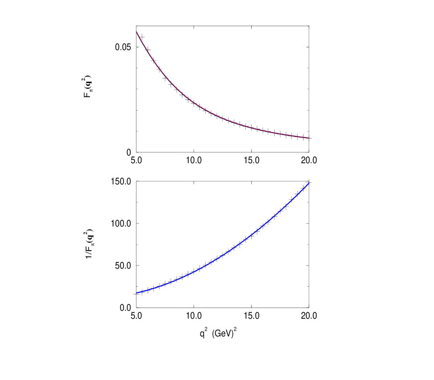
Figure 5: The upper panel compares $F_{\pi}(q^{2})$ with the reciprocal of the fitting function. The $a_{2}$ term provides more than 60% of the value of $F_{\pi}(q^{2})$ only for $q^{2}>10$ GeV². The lower panel compares $1/F_{\pi}(q^{2})$ (plotted points) with the fitting function of Eq. (60).

Equation (58) follows because of the constraints that the realisation of confinement explored herein place on the fermion propagator. This mechanism is not an essential element of the DSE framework. The invalidity of Eq. (58), and hence Eq. (59), would not compromise the quantitative results discussed in the preceding sections.

6 Summary and Conclusions

The impulse approximation, illustrated in Fig. 1, has been used to calculate $F_{\pi}(q^{2})$ at spacelike-$q^{2}$; i.e., away from resonance contributions. The important elements of this calculation are: the dressed quark propagator; the pion Bethe-Salpeter amplitude; and the dressed quark-photon vertex, which follow from realistic, nonperturbative Dyson-Schwinger equation studies. This entails that in this calculation each of these elements behaves at large spacelike-$p^{2}$ in the manner prescribed by the renormalisation group in QCD, up to $\ln[p^{2}]$-corrections, and at small spacelike-$p^{2}$ in such a way as to ensure confinement. In addition, the same approach has been used to simultaneously calculate: $f_{\pi}$; $m_{\pi}$; $\langle\bar{q}q\rangle$; $r_{\pi}$; the $\pi^{0}\rightarrow\gamma\gamma$ decay width; the $\pi$-$\pi$ scattering lengths: $a_{0}^{0}$, $a_{0}^{2}$, $a_{1}^{1}$, $a_{2}^{0}$, $a_{2}^{2}$; and the associated partial wave amplitudes.

The calculated results for all quantities agree well with the data, as discussed in Sec. 4.2. This supports the contention that the confined, nonperturbative “dressed-quark core” is the dominant determining characteristic of the pion, away from resonance contributions. Particularly interesting in this context is the calculation of the $\pi^{0}\rightarrow\gamma\gamma$ decay width, Sec. 3. The correct chiral limit value for this decay width is obtained independent of the details of the modelling of the quark propagator. This is an illustration of the manner in which the Abelian anomaly manifests itself in the Dyson-Schwinger equation approach. This calculation indicates that soft, nonperturbative contributions dominate the exclusive electromagnetic form factor for spacelike-$q^{2}\mathrel{\hbox to0.0pt{\lower 4.0pt\hbox{\hskip 1.0pt$\sim$}\hss}\raise 1.0pt\hbox{$<$}}10$ GeV².

The Dyson-Schwinger equation approach provides a phenomenological framework in which to relate experimental observables to the qualitative and quantitative features of the effective quark-quark interaction in the infrared, which is an important but presently unknown aspect of QCD. There have been attempts to calculate the gluon propagator directly: some by solving the Dyson-Schwinger equation for the gluon vacuum polarisation [15, 16, 17]; and others via lattice simulations [40], which are presently qualitatively and quantitatively unreliable for spacelike-$q^{2}\mathrel{\hbox to0.0pt{\lower 4.0pt\hbox{\hskip 1.0pt$\sim$}\hss}\raise 1.0pt\hbox{$<$}}1$ GeV². The present study suggests that the framework explored herein can be a valuable complement to such analyses. More precise measurements of $F_{\pi}(q^{2})$ for spacelike-$q^{2}\mathrel{\hbox to0.0pt{\lower 4.0pt\hbox{\hskip 1.0pt$\sim$}\hss}\raise 1.0pt\hbox{$>$}}1$ GeV² would be useful in this regard.

Acknowledgments.
This work was supported by the US Department of Energy, Nuclear Physics Division, under contract number W-31-109-ENG-38. The calculations described herein were carried out using a grant of computer time and the resources of the National Energy Research Supercomputer Center.

References

• [EMail] cdroberts@anl.gov
• [1] P. L. Chung, F. Coester and W. N. Polyzou, Phys. Lett. B 205 (1988) 545.
• [2] K. Langfeld, R. Alkofer and P. A. Amundsen, Z. Phys. C. 42 (1989) 159.
• [3] H. Ito, W. W. Buck and F. Gross, Phys. Lett. B 248 (1990) 28.
• [4] A. V. Efremov and A. V. Radyushkin, Phys. Lett. B 94 (1980) 245; G. P. Lepage and S. J. Brodsky, Phys. Rev. D 22 (1980) 2157.
• [5] N. Isgur and C. H. Llewellyn Smith, Phys. Rev. Lett. 52 (1984) 1080; Nucl. Phys. B 317 (1989) 526.
• [6] A. Szczepaniak and A. G. Williams, Phys. Lett. B 302 (1993) 87.
• [7] C. D. Roberts and A. G. Williams, Prog. Part. Nucl. Phys., 33 (1994) 477.
• [8] R. Delbourgo and M. D. Scadron, J. Phys. G 5 (1979) 1631.
• [9] J. S. Ball and T.-W. Chiu, Phys. Rev. D 22 (1980) 2542.
• [10] D. C. Curtis and M. R. Pennington, Phys. Rev. D 46 (1992) 2663; A. Bashir and M. R. Pennington, Phys. Rev. D 50 (1994) 7679.
• [11] C.ย J.ย Burden and C.ย D.ย Roberts, Phys. Rev. D 47 (1993) 5581; Z. Dong, H. J. Munczek and C. D. Roberts, Phys. Lett. B 333 (1994) 536.
• [12] C. D. Roberts, A. G. Williams and G. Krein, Intern. J. Mod. Phys. A 7 (1992) 5607.
• [13] M. R. Frank and P. C. Tandy, Phys. Rev. C 49 (1994) 478.
• [14] C.ย J.ย Burden, C.ย D.ย Roberts and A.ย G.ย Williams, Phys. Lett. B 285 (1992) 347.
• [15] M. Baker, J. S. Ball and F. Zachariasen, Nucl. Phys. B 186 (1981) 531; ibid 560.
• [16] D. Atkinson, P. W. Johnson, W. J. Schoenmaker and H. A. Slim, Nuovo Cim. A 77 (1983) 197.
• [17] N. Brown and M. R. Pennington, Phys. Lett. B 202, 257 (1988); Phys. Rev. D 38 (1988) 2266.
• [18] G. V. Efimov and M. A. Ivanov, The Quark Confinement Model of Hadrons (IOP Publishing, 1993).
• [19] H. D. Politzer, Nucl. Phys. B 117 (1982) 397.
• [20] A.ย G.ย Williams, G.ย Krein and C.ย D.ย Roberts, Ann. Phys. (NY) 210 (1991) 464.
• [21] K. L. Mitchell, P. C. Tandy, C. D. Roberts and R. T. Cahill, Phys. Lett. B 335 (1994) 282.
• [22] P. Jain and H. Munczek, Phys. Rev. D 48 (1993) 5403 and references therein.
• [23] C. H. Llewellyn-Smith, Ann. Phys. (N.Y.) 53 (1969) 521.
• [24] V. A. Miransky, Mod. Phys. Lett A 5 (1990) 1979.
• [25] M. R. Frank and C. D. Roberts, Phys. Rev. C 53 (1996) 390.
• [26] M. R. Frank, Phys. Rev. C 51 (1995) 987.
• [27] R. Alkofer, A. Bender and C. D. Roberts, Intern. J. Mod. Phys. A 10, Vol. 23 (1995) 3319.
• [28] C. D. Roberts, R. T. Cahill and J. Praschifka, Ann. Phys. 188 (1988) 20.
• [29] R. Alkofer and C. D. Roberts, Phys. Lett. B 369 (1996) 101.
• [30] C. D. Roberts, R. T. Cahill, M. E. Sevior and N. Iannella, Phys. Rev. D 49 (1994) 125.
• [31] D. Pocaniฤ‡, โ€œChiral Dynamics: Theory and Experimentโ€, A. M. Bernstein and B. R. Holstein (Eds.), Lecture Notes in Physics, Vol 452, p. 95 (Springer, Berlin 1995).
• [32] Particle Data Group, Phys. Rev. D 45 (1992) S1.
• [33] S. R. Amendolia, et al, Nucl. Phys. B 277 (1986) 168.
• [34] S. Weinberg, Phys. Rev. Lett. 17 (1966) 616.
• [35] C. N. Brown, et al, Phys. Rev. D 8 (1973) 92.
• [36] C. J. Bebek, et al, Phys. Rev. D 13 (1976) 25.
• [37] C. J. Bebek, et al, Phys. Rev. D 17 (1978) 1693.
• [38] C.ย D.ย Roberts and B.ย H.ย J.ย McKellar, Phys. Rev. D 41 (1990) 672; H. J. Munczek and D. W. McKay, Phys. Rev. D 42 (1990) 3548.
• [39] M. V. Terentโ€™ev, Yad. Fiz. 24 (1976) 207 [Sov. J. Nucl. Phys. 24 (1976) 106].
• [40] C. Bernard, C. Parrinello and A. Soni, Phys. Rev. D 49 (1994) 1585.