KUNS-1278

HE(TH) 94/10

NIIG-DP-94-2

hep-ph/9407398

July, 1994

Nontriviality of Gauge-Higgs-Yukawa System and Renormalizability of Gauged NJL Model

Masayasu Harada, Yoshio Kikukawa, Taichiro Kugo

Department of Physics, Kyoto University, Kyoto 606-01, Japan

and

Hiroaki Nakano

Department of Physics, Niigata University, Niigata 950-21, Japan

In the leading order of a modified $1/N_{\rm C}$ expansion, we show that a class of gauge-Higgs-Yukawa systems in four dimensions give non-trivial and well-defined theories in the continuum limit. The renormalized Yukawa coupling $y$ and the quartic scalar coupling $\lambda$ have to lie on a certain line in the $(y,\lambda)$ plane and the line terminates at an upper bound. The gauged Nambu–Jona-Lasinio (NJL) model in the limit of its ultraviolet cutoff going to infinity, is shown to become equivalent to the gauge-Higgs-Yukawa system with the coupling constants just on that terminating point. This proves the renormalizability of the gauged NJL model in four dimensions. The effective potential for the gauged NJL model is calculated by using renormalization group technique and confirmed to be consistent with the previous result by Kondo, Tanabashi and Yamawaki obtained by the ladder Schwinger-Dyson equation.

1 Introduction

It is generally a difficult problem whether a theory defined with an ultraviolet cutoff (such as in lattice formulation) really has a well-defined (i.e., finite) continuum limit which is not a free theory. If the theory becomes necessarily free in the continuum limit, the theory is called trivial and if it gives an interacting theory, it is called nontrivial. This triviality or nontriviality is always a problem independently of whether the theory is perturbatively renormalizable or not. But, if a theory is perturbatively non-renormalizable and nevertheless gives a nontrivial continuum limit, people prefer to call it (non-perturbatively) renormalizable rather than simply calling it nontrivial. We also follow this terminology in this paper.

We discuss two problems in this paper. One is the triviality problem of a class of gauge-Higgs-Yukawa systems in four dimensions which are of course (perturbatively) renormalizable. We examine and clarify when they can give well-defined, nontrivial theories in the continuum limit (i.e., when the ultraviolet cutoff goes to infinity). Another is the renormalizability of gauged Nambu–Jona-Lasinio (NJL) models in four dimensions which are (perturbatively) non-renormalizable. We note that the gauged NJL models are equivalent to special cases of gauge-Higgs-Yukawa systems at the stage with the ultraviolet cutoff kept finite. Considering the limit of the cutoff going to infinity, we can show that, under a certain condition, the gauged NJL models give well-defined continuum limits which are equivalent to specific nontrivial gauge-Higgs-Yukawa theories. Namely, gauged NJL models become renormalizable in the sense of above terminology.

Kondo, Tanabashi and Yamawaki[1] (KTY) have studied the gauged NJL model for the fixed (non-running) gauge coupling case and have shown the renormalizability within the ladder approximation of the Schwinger-Dyson (SD) equation. This conclusion has further been supported by their recent work with Shibata[2] in which they analyzed the flow of the renormalized Yukawa coupling and mass parameter in the corresponding gauge-Higgs-Yukawa theory. These works are, however, restricted to the fixed gauge coupling case, and moreover their arguments are based on a particular technique of ladder SD equation whose nature of approximation is rather unclear. It is therefore necessary to do clearer analysis based on a more sound technique. We adopt the renormalization group equation (RGE) as our basic tool in this paper and directly examine them in a definite approximation scheme.

We spell out here about an assumption we take. For the present purpose, we should ideally analyze the RGE’s in a Wilson’s sense[3] which trace the RG flow of the coupling constants of the cutoff theories. However, we actually do not work directly in the cutoff theories. Instead, we analyze the RGE’s in the continuum theories, but assume that the coupling constants renormalized at $\mu$ there can be identified with the bare coupling constants in the cutoff theory with cutoff $\Lambda=\mu$, at least when the renormalization point $\mu$ becomes very large. The validity of this assumption, however, would generally depend on how the renormalized coupling constants are defined in the continuum theory. The authors of ref. [4] have explicitly worked out on this point in a Higgs-Yukawa system and seen the following: such identification is valid for coupling constants corresponding to operators of dimension four. But a care had to be taken for the mass parameter to which quadratic divergences are relevant. We should use the mass parameter in the mass-dependent renormalization scheme in order to identify it with that in the cutoff theory. Our assumption here is that the situation is the same also in the present gauged Higgs-Yukawa systems.

To analyze the above stated problems, we work in the leading order in $1/N_{\rm C}$ expansion combined with the perturbation with respect to a small, asymptotically free gauge coupling constant $g^{2}$. We also use an additional assumption that the pure $\lambda\phi^{4}$ theory is trivial[5]. Then we show that the followings should hold in order for the gauge-Higgs-Yukawa system to give a nontrivial and well-defined theory. (i) There exists a functional relation between the renormalized Yukawa coupling $y(\mu)$ and quartic scalar coupling $\lambda(\mu)$. Namely, these couplings should lie on a certain line in the $(y,\lambda)$ plane. (ii) There exists a nonzero, finite upper bound for the renormalized Yukawa coupling. The line in the $(y,\lambda)$ plane terminates at the upper bound. This upper bound corresponds to the infrared ‘fixed point’ of Pendleton and Ross (PR)[6].

Based on these results, we turn to the analysis of the gauged NJL model. We make use of the compositeness condition which relates the gauged NJL model to a gauge-Higgs-Yukawa system, and show that (iii) the gauged NJL model is renormalizable if and only if the equivalent gauge-Higgs-Yukawa system approaches the PR fixed point in the continuum limit. Furthermore, we calculate the effective potential of the renormalizable gauged NJL model by using RGE technique and explicitly perform the renormalization of it. We find that (iv) the resultant expression for the effective potential is consistent with the previous result by KTY[1], a renormalized form of Bardeen-Love’s[7] potential, which was obtained in the fixed gauge coupling case by solving SD equation in the ladder approximation.

For the nontriviality of gauge-Higgs-Yukawa systems and hence for the renormalizability of gauged NJL model, the presence of asymptotically free (or fixed coupling) gauge interaction is essential. It also turns out that (v) the asymptotic freedom of the gauge interaction should not be too strong.

We note that these points (iii) and (v) were in fact suggested by Kondo, Shuto and Yamawaki[8]. They calculated the decay constant $F_{\pi}$ using the ladder SD equation and the Pagels-Stokar formula, and observed that $F_{\pi}$ (and hence the Yukawa coupling) can be finite in the presence of weakly-asymptotic-free gauge interaction. Based on this observation, they suggested that the gauge interaction might promote the trivial NJL model to an interacting renormalizable theory.

These points (iii) and (v) were also claimed by Krasnikov[10] who discussed the problem in the gauged NJL model in $4-\epsilon$ dimensions. Although his argument based on RGE’s is similar to ours and very suggestive for the possible existence of the theory, he discussed neither the compositeness condition nor the relation between the gauged NJL model and the gauge-Higgs-Yukawa system at the regularized level with a finite cutoff $\Lambda$ (or finite $\epsilon$). Consequently it was left unclear how to take the continuum limit, i.e., how to renormalize the gauged NJL model.

The paper is organized as follows. In the next section, we describe the nature of our approximation and solve the RGE’s for the Yukawa and quartic scalar couplings as well as the gauge coupling in the continuum gauge-Higgs-Yukawa system. The solutions are characterized by some RG invariants. In section 3, after presenting our criteria for nontriviality, we show the above two points (i) and (ii). The analysis of gauged NJL model is performed in sections 4 to 6. In section 4, we impose compositeness conditions on the Yukawa and quartic scalar coupling constants in the gauge-Higgs-Yukawa system to relate it to the gauged NJL model, and prove the above point (iii), i.e., the renormalizability of the gauged NJL model. To make the connection between the two systems complete, it is necessary to discuss another compositeness condition on the mass parameter. We discuss this condition in detail in section 5 since it is important to see how the four fermion interaction $G$ determines the phase structure of the equivalent gauge-Higgs-Yukawa system. Based on this, we calculate the effective potential of the gauged NJL model and renormalize it explicitly in section 6. The final section is devoted to conclusions.

2 Renormalization Group Equations

We consider the Higgs-Yukawa theory with $SU(N_{\rm C})$ color gauge interaction, which contains $N_{\rm f}$ species of colored fermions $\psi_{i}$ ($i=1$ – $N_{\rm f}$), each belonging to a representation $R$ of $SU(N_{\rm C})$, and a color-singlet scalar field $\sigma$. In this paper, we work in the leading order of $1/N_{\rm C}$ expansion in the following sense. Usually in the leading order of $1/N_{\rm C}$ expansion, all the planar diagrams contribute to the renormalization group equation. However, we are interested in the high-energy asymptotic region where the QCD gauge coupling $g$ is small enough to be treated perturbatively; $N_{\rm C}g^{2}/4\pi\ll 1$. We will work in the first nontrivial order in the gauge coupling expansion. Moreover, we consider the case where there exist large number of fermions in the theory, so we regards $N_{\rm f}\sim N_{\rm C}$. However, only $n_{\rm f}$ fermions $\psi_{i}$ ($i=1$ – $n_{\rm f}\ll N_{\rm f}$) among them have a degenerate large Yukawa coupling, while the others have vanishing or negligibly small Yukawa couplings. As such, the Lagrangian we consider in this paper is given by

$${\cal L}_{\rm gHY}~{}~{}= - \!\!\!\frac{1}{4}\left(F_{\mu\nu}\right)^{2}+\frac{1}{2}\left(\partial_{\mu}\sigma\right)^{2}-\frac{1}{2}m^{2}\sigma^{2}-\frac{\lambda}{4}\sigma^{4}$$ (2.1)

$$+ \!\!\!\sum_{i=1}^{N_{\rm f}}\overline{\psi_{i}}\,i\,\hbox to0.0pt{/\hss}\!D\psi_{i}-\sum_{i=1}^{n_{\rm f}}y\sigma\overline{\psi}_{i}\psi_{i}\ ,$$

where $D_{\mu}$ is a color-covariant derivative and $y$ and $\lambda$ are the Yukawa and quartic scalar coupling constants, respectively. This choice of model is obviously inspired by the minimal Standard Model (SM) where $N_{\rm C}=N_{\rm f}/2=3$ and $n_{\rm f}=1$. We note, however, that the present system crucially differs from the SM in that the asymptotically nonfree $U(1)$ gauge interaction is switched off.

Let $\mu_{0}$ denote a reference scale at which we discuss the low-energy physics, and $t\equiv\ln(\mu/\mu_{0})$ where $\mu\,(>\Lambda_{{\rm QCD}})$ is the renormalization point. RGE’s for the gauge coupling $g(t)$, the Yukawa coupling $y(t)$ and the quartic scalar coupling $\lambda(t)$ are given in the leading order of our approximation by

$$16\pi^{2}\frac{d}{dt}g(t) = -bg^{3}(t)\ ,$$ (2.2)

$$16\pi^{2}\frac{d}{dt}y(t) = y(t)\left[ay^{2}(t)-cg^{2}(t)\right]\ ,$$ (2.3)

$$16\pi^{2}\frac{d}{dt}\lambda(t) = uy^{2}(t)\left[\lambda(t)-vy^{2}(t)\right]\ ,$$ (2.4)

with $b$, $a$, $c$, $u$ and $v$ being positive constants:

$$b=\frac{11N_{\rm C}-4T(R)N_{\rm f}}{3},\quad c=6C_{2}(R),\quad a=\frac{u}{4}=2n_{\rm f}N_{\rm C},\quad v=1\ ,$$ (2.5)

where $C_{2}(R)$ is a second Casimir, and $T(R)=1/2$ and $C_{2}(R)=(N_{\rm C}^{2}-1)/(2N_{\rm C})$ when $R$ is the fundamental representation. [We can also consider the fixed gauge coupling case, by taking the limit $b\rightarrow+0$.] Note that in the $1/N_{\rm C}$ leading approximation, $u=4a$ independently of the model’s detail since both $a$ and $u$ are determined solely by the fermion one-loop contribution to the scalar self-energy.

It will be important to note that aside from the perturbation with respect to the gauge coupling, we are working in the leading order in $1/N_{\rm C}$ expansion and hence neglecting the scalar loop contributions. The latter approximation is valid as long as the quartic scalar coupling $\lambda$ is small compared with $N_{\rm C}y^{2}$:

$$\left|{\frac{\lambda\,}{\,y^{2}}}\right|\mathrel{\mathchoice{\vbox{\offinterlineskip\halign{$\m@th\displaystyle\hfil#\hfil$\cr<\crcr\sim\crcr} }}{\vbox{\offinterlineskip\halign{$\m@th\textstyle\hfil#\hfil$\cr<\crcr\sim\crcr} }}{\vbox{\offinterlineskip\halign{$\m@th\scriptstyle\hfil#\hfil$\cr<\crcr\sim\crcr} }}{\vbox{\offinterlineskip\halign{$\m@th\scriptscriptstyle\hfil#\hfil$\cr<\crcr\sim\crcr} }}}N_{\rm C}\ .$$ (2.6)

But if we follow the flow determined by the RGE (2.4) in $1/N_{\rm C}$ leading order, we often reach the region in which this condition breaks down. In such a situation, we should include the scalar loop contributions beyond the $1/N_{\rm C}$ leading order. For instance in the one-loop order, the RGE (2.4) should be replaced by an equation of the form

$$16\pi^{2}\frac{d}{dt}\lambda(t)=w\lambda^{2}+uy^{2}(t)\left[\lambda(t)-vy^{2}(t)\right]$$ (2.7)

where $w>0$ is a constant of order $1$, while $u$ and $v$ are the same as before. We shall come back to this point in the next section.

Let us now solve the RGE’s (2.2)–(2.4) and analyze the solution. The solution to Eq. (2.2) for the gauge coupling $\alpha=g^{2}/(4\pi)$ is well-known:

$$\eta(t)\equiv\frac{g^{2}(t)}{g^{2}_{0}}\equiv\frac{\alpha(t)}{\alpha_{0}}=\left(1+\frac{b\alpha_{0}}{2\pi}t\right)^{-1}\ ,$$ (2.8)

where coupling constants with subscript $0$ generally denote the initial values at the reference scale $\mu_{0}$; e.g., $\alpha_{0}=\alpha(t\!=\!0)$. Note that $\eta(0)=1$, and $\eta(t)\rightarrow+0$ in the ultraviolet (UV) limit $t\rightarrow+\infty$.

The simplest way to solve the RGE’s (2.3) and (2.4) is to observe that the quantities

$$h(t) \equiv -\eta^{-1+c/b}(t)\left[1-\frac{c-b}{a}\frac{g^{2}(t)}{y^{2}(t)}\right]\ ,$$ (2.9)

$$k(t) \equiv -\eta^{-1+2c/b}(t)\left[1-\frac{2c-b}{2av}\frac{\lambda(t)}{y^{2}(t)}\frac{g^{2}(t)}{y^{2}(t)}\right]$$ (2.10)

are RG invariant: $0=(d/dt)h(t)=(d/dt)k(t)$. Then the solutions of the RGE’s are specified once the values of the RG invariants $h$ and $k$ are given. Let $h_{0}$ and $k_{0}$ denote the values of the invariants. Then we can write the solutions as

$$y^{2}(t) = \frac{c-b}{a}g^{2}(t)\left[1+h_{0}\eta^{1-c/b}(t)\right]^{-1}\ ,$$ (2.11)

$$\lambda(t) = \frac{2av}{2c-b}\frac{y^{4}(t)}{g^{2}(t)}\left[1+k_{0}\eta^{1-2c/b}(t)\right]\ .$$ (2.12)

Before entering the detailed analysis in the next section, let us briefly see how the solutions look like in some limiting cases. First, the fixed gauge coupling limit $b\rightarrow+0$ can be taken by using

$$\eta^{-c/b}(t)\mathop{\ \longrightarrow\ }_{b\rightarrow 0}\exp{\left(\frac{\alpha}{\alpha_{\rm c}}t\right)}=\left(\frac{\mu\,}{\,\mu_{0}}\right)^{\alpha/\alpha_{\rm c}},$$ (2.13)

where $\alpha\,(=\alpha_{0})$ is the fixed gauge coupling constant and

$$\frac{1}{\alpha_{\rm c}}\equiv\frac{c}{2\pi}=\frac{3C_{2}(R)}{\pi}\ .$$ (2.14)

Then we obtain from Eqs. (2.11) and (2.12)

$$y^{2}(t) = \frac{(4\pi)^{2}}{2a}\frac{\alpha}{\alpha_{\rm c}}\left[1+h_{0}\exp\left(\frac{\alpha}{\alpha_{\rm c}}t\right)\right]^{-1}\ ,$$ (2.15)

$$\lambda(t) = \frac{2av}{(4\pi)^{2}}\frac{\alpha_{\rm c}}{\alpha}y^{4}(t)\left[1+k_{0}\exp\left(\frac{2\alpha}{\alpha_{\rm c}}t\right)\right]\ .$$ (2.16)

Next we consider the limiting case $b=c$. Although the Yukawa coupling (2.11) appears to vanish in this case, a careful consideration of RGE leads to a non-vanishing result. The correct way is first to write the RG invariant as

$$h_{0}=-1+\frac{c-b}{b}h_{1}$$ (2.17)

and then to take the limit $c\rightarrow b$ in Eq. (2.11). Then we find that

$$y^{2}(t)=\frac{b}{a}g^{2}(t)\left[h_{1}+\ln\eta(t)\right]^{-1}\ .$$ (2.18)

Note that $h_{1}=(b/a)(g^{2}_{0}/y^{2}_{0})$ is RG invariant in this limiting case. The case $b=2c$ can be treated in a similar manner.

3 Nontriviality of Gauge-Higgs-Yukawa System

We now use the solutions of the RGE’s found in the preceding section to investigate under what circumstances the gauge-Higgs-Yukawa system is nontrivial. We adopt the following criteria for the nontriviality: all the running coupling constants should not diverge at any finite $t$($>0$), should not vanish identically and should not violate the consistency of the theory, such as the unitarity and vacuum stability. Note that we are demanding the nontriviality as a gauge-Higgs-Yukawa system. Namely, for instance, we do not call nontrivial the system with $y(t)\equiv\lambda(t)\equiv 0$, which is in fact a nontrivial QCD-like theory with the scalar field decoupled completely. Note also that the mass parameter poses no problem, since it is multiplicatively renormalized in the $\overline{\rm MS}$ scheme. Even if the multiplicative factor diverges at a finite $t$, we can avoid the problem by setting $m^{2}\equiv 0$ and it does not imply the triviality of the theory.

We should remark that we are restricting ourselves only to the cases where the gauge coupling remains small in the UV region. If the Yukawa or quartic scalar couplings become so large that the $1/N_{\rm C}$ expansion breaks down, they might affect the behavior of $g^{2}(t)$ substantially such that our perturbation assumption with respect to $g^{2}(t)$ is violated. So, logically, there remain possibilities that all the couplings become large but have a nontrivial UV fixed point so that the system gives a nontrivial theory. This is outside the scope of this paper.

3.1 Fixed Point Solution

It is instructive to analyze first the case in which the RG invariants are $h_{0}=k_{0}=0$. In this case, the solutions (2.11) and (2.12) reduce to

$$\frac{y^{2}(t)}{g^{2}(t)} = \frac{c-b}{a}\ ,$$ (3.1)

$$\frac{\lambda(t)}{y^{2}(t)} = \frac{2av}{2c-b}\frac{y^{2}(t)}{g^{2}(t)}=\frac{2v\,(c-b)}{2c-b}\ .$$ (3.2)

We see that the behavior of the Yukawa and quartic scalar couplings, $y(t)$ and $\lambda(t)$, are completely determined by that of the gauge coupling $g(t)$. This corresponds to the “coupling constant reduction” in the sense of Kubo, Sibold and Zimmermann[11]. In the context of RGE, it corresponds to the Pendleton-Ross (PR) fixed point[6]. This can be seen by rewriting the RGE’s (2.2)–(2.4) into

$$8\pi^{2}\frac{d}{dt}\left[\frac{y^{2}(t)}{g^{2}(t)}\right] = ag^{2}(t)\left[\frac{y^{2}(t)}{g^{2}(t)}\right]\left[\frac{y^{2}(t)}{g^{2}(t)}-\frac{c-b}{a}\right]\ ,$$ (3.3)

$$8\pi^{2}\frac{d}{dt}\left[\frac{g^{2}(t)}{y^{2}(t)}\frac{\lambda(t)}{y^{2}(t)}\right] = (2c-b)g^{2}(t)\left[\frac{g^{2}(t)}{y^{2}(t)}\frac{\lambda(t)}{y^{2}(t)}-\frac{2av}{2c-b}\right]\ .$$ (3.4)

Clearly, the solution $h_{0}=0$ and $k_{0}=0$ is the fixed point of the RGE’s (3.3) and (3.4). [Note that the former RGE has two fixed points, i.e., $y^{2}/g^{2}=0$ and the PR fixed point $y^{2}/g^{2}=(c-b)/a$.]

Observe that the expressions (3.1) and (3.2) make sense only when $c\geq b$. [Otherwise, the Yukawa coupling becomes complex implying the violation of unitarity, or the quartic scalar coupling becomes negative implying the instability of the vacuum.] When $c>b$, the Yukawa and quartic scalar couplings as well as the gauge coupling are asymptotically free. This is a sufficient condition for the nontriviality of this system. [The case $c=b$ requires some caution and will be discussed later.]

We thus see that if $c>b$, the gauge-Higgs-Yukawa system with $h_{0}=k_{0}=0$ corresponds to the PR fixed point solution to the RGE’s and hence a nontrivial theory. This consideration also clarifies the meaning of the RG invariants $h_{0}$ and $k_{0}$; they characterize how much the RG flow deviates from the PR one. Then the next question will be how about the case $h_{0}\neq 0$ or $k_{0}\neq 0$. We will systematically explore this in the following.

3.2 Yukawa Coupling

Let us first discuss the Yukawa coupling $y(t)$. As we have seen in the preceding subsection, the behavior of the Yukawa coupling will be quite different depending on whether $c>b$ or $c<b$. Also the case $c=b$ requires a special care. Moreover, the sign of the RG invariant $h_{0}$ will be important. We proceed in the order i) $c>b$, ii) $c<b$, iii) $c=b$. It will turns out that the Yukawa interaction can be nontrivial only for the first case $c>b$.

3.2.1 $c>b$ case

Let us start with the case $c>b$. Since $\eta^{1-c/b}(t)$ becomes large as $t\rightarrow+\infty$, the UV asymptotic behavior of $y^{2}(t)$ in Eq. (2.11) is given by

$$y^{2}(t)\sim\frac{c-b}{a}\frac{g^{2}_{0}}{h_{0}}\eta^{c/b}(t)\ \longrightarrow\ \pm 0\ .$$ (3.5)

Then it appears that the Yukawa coupling is asymptotically free and the theory is nontrivial in this case. However, the sign of the RG invariant $h_{0}$ is crucial in order that this is really true.

For $0<h_{0}<+\infty$, we see from the solution (2.11) that $y^{2}(t)$ remains positive and finite. Then the UV asymptotic behavior is really given by Eq. (3.5), $y^{2}(t)\rightarrow+0$, and the theory is nontrivial.

For $-\infty<h_{0}<0$, however, this is not the case. First of all, notice that we should exclude $h_{0}\leq-1$ from the beginning in order that $y^{2}_{0}\equiv y^{2}(t\!=\!0)$ is finite and positive. Even for $-1<h_{0}<0$, there exists a Landau pole at a finite value of $t>0$ satisfying

$$1+\frac{b\alpha_{0}}{2\pi}t=\left(\frac{-1}{h_{0}}\right)^{b/(c-b)}$$ (3.6)

at which $y^{2}(t)$ diverges and changes its sign. So even if $y^{2}_{0}$ is arranged to be positive and finite at an infrared (IR) scale $\mu_{0}$, such a property is not preserved in the UV region. The asymptotic behavior (3.5) holds in the UV region beyond the Landau pole, but the unitarity is violated there. Thus the theory is trivial according to our criteria.

The RG flows in the $(\alpha,y^{2})$ plane are shown in Fig. 1.

Figure 1: RG flows in the $(\alpha,y^{2})$ plane. The arrows denote the flow directions toward the UV region. The flows for $h_{0}\geq 0$ below the $h_{0}=0$ line all converge to the origin (i.e., asymptotically free) while those for $h_{0}<0$ diverge at finite $t$ (or $\alpha$).

In this way we conclude that the Yukawa interaction with $c>b$ is nontrivial if and only if $h_{0}\geq 0$. Note that the nontriviality does not necessarily imply the coupling reduction: there exist a one parameter family of theories ($0<h_{0}<+\infty$) which do not correspond to the PR fixed point ($h_{0}=0$). Indeed, the value of the Yukawa coupling $y^{2}_{0}$ at the IR scale $\mu_{0}$ is given by

$$0\ <\ \ y^{2}_{0}=\frac{1}{1+h_{0}}\frac{c-b}{a}g^{2}_{0}\ \ \leq\ \ \frac{c-b}{a}g^{2}_{0}\equiv y^{2}_{\star}\ .$$ (3.7)

We see that the low-energy Yukawa coupling $y^{2}_{0}$ can take any value in between $0$ and $y^{2}_{\star}$, and that the upper bound $y^{2}_{\star}$ is given by the PR fixed point (3.1).

3.2.2 $c<b$ case

In this case of $c<b$, $\eta^{1-c/b}(t)\rightarrow+0$, and the UV asymptotic behavior of the solution (2.11) is given, instead of (3.5), by

$$y^{2}(t)\ \sim\ -\frac{b-c}{a}g^{2}(t)\ \ \longrightarrow\ \ -0\ .$$ (3.8)

Since the RHS of this equation is negative, there is no chance for us to have a nontrivial theory in this case.

Indeed, for $0\leq h_{0}<+\infty$, $y^{2}(t)$ is always negative, and the unitarity is violated although there is no Landau pole. For $-\infty<h_{0}<0$, we meet a Landau pole; even if $y^{2}_{0}$ is arranged to be finite and positive, $y^{2}(t)$ diverges at finite $t$.

It would be amusing, however, to note that this case $c<b$ can be related to the above case of $c>b$ by the following ‘symmetry’ of the RGE’s under the transformation $(t,y,b,c)\rightarrow(-t,iy,-b,-c)$ with others inert. This exchanges the UV with the IR region, and $c>b$ with $c<b$ case. We then find that the nontrivial theory with $c>b$ and $h_{0}\geq 0$ in the physical region $y^{2}>0$ is mapped to the theory with $c<b$ and $h_{0}\geq 0$ in the unphysical region $y^{2}<0$.

3.2.3 $c=b$ case

In this case, we should use the solution (2.18) with $h_{1}$ given in Eq. (2.17). Since $\ln\eta(t)$ behaves like $-\ln t$ as $t\rightarrow+\infty$, the UV asymptotic behavior is

$$y^{2}(t)=\frac{b}{a}g^{2}(t)\left[h_{1}-\ln\left(1+\frac{b\alpha_{0}}{2\pi}t\right)\right]^{-1}\ \longrightarrow\ -\frac{b}{a}\frac{g^{2}(t)}{\ln t}\ .$$ (3.9)

Then as in the case $c<b$, we find that the Yukawa coupling $y^{2}(t)$ is always negative for $h_{1}\leq 0$, and that for $h_{1}>0$ it always has a Landau pole at $\ln(1+b\alpha_{0}t/2\pi)=h_{1}$.

Combined with the result for the case $c<b$, we conclude that the Yukawa interaction with $c\leq b$ is necessarily trivial.

3.2.4 Further Comments

It is well known that the Yukawa interaction is trivial by itself since the RGE (2.3) without $g^{2}$ is easily solved to produce a Landau pole. For the existence of the nontrivial Yukawa interaction, the presence of asymptotically free (or fixed coupling) gauge interaction, $b\geq 0$, is crucial. Our result, however, shows that $b$ should be smaller than $c$; the asymptotic freedom of gauge interaction should not be too strong. Let us now think about the reason.

For a moment, let us go back to the original RGE (2.3). Based on this equation, one might expect that the Yukawa interaction would be nontrivial if

$$y^{2}_{0}\leq\frac{c}{a}g^{2}_{0}\ ,$$ (3.10)

since the RGE (2.3) has an IR-stable ‘fixed point’ $y^{2}=(c/a)g^{2}$ of order $O(g^{2})$; If this condition is satisfied at some scale, the Yukawa coupling has negative beta function and seems asymptotically free. The point is, however, that the ‘fixed point’ itself moves to zero as $t$ becomes large, and it will ‘overtake’ the Yukawa coupling $y^{2}(t)$ when the asymptotic freedom of gauge interaction is too strong. The condition (3.10) is necessary, but not sufficient in order for the theory to give really an asymptotically free theory. The argument based on the exact solution (2.11) shows that the sufficient condition is given by Eq. (3.7). This in turn implies that $b$ should be positive, but not too much.

This fact was originally pointed out by Krasnikov[10] from the analysis of the RGE’s in the one-loop order. His conclusion was that there exists a minimal number for the colored fermions which weaken the asymptotic freedom of QCD gauge interaction. In our case with RGE’s in the $1/N_{\rm C}$-leading order, we have modified the $1/N_{\rm C}$ expansion by including the $N_{\rm f}\sim N_{\rm C}$ species of fermions. For instance, if $N_{\rm f}\simeq 2N_{\rm C}$ and $R$ is the fundamental representation, then $c\simeq 3N_{\rm C}$ and $b\simeq(7/3)N_{\rm C}$, and hence the condition $c>b>0$ is satisfied.

Finally it is interesting to note that the Standard Model with three generations of fermions (with $SU(2)_{\rm L}\times U(1)_{\rm Y}$ gauge interactions switched off) just gives an example of this category of theories, so that it would nontrivially exist even when the cutoff goes to infinity.

3.3 Quartic Scalar Coupling

We now proceed to analyze the quartic scalar coupling $\lambda(t)$. We restrict ourselves to the case of $c>b$ and $h_{0}\geq 0$ in which a nontrivial limit of Yukawa coupling can be taken.

The solution (2.12) explicitly reads

$$\lambda(t)=\frac{2v\,(c-b)^{2}}{a\,(2c-b)}g^{2}_{0}\eta(t)\frac{1+k_{0}\eta^{1-2c/b}(t)}{\left[1+h_{0}\eta^{1-c/b}(t)\right]^{2}}\ .$$ (3.11)

When $k_{0}=0$, the asymptotic behavior in the UV limit $\eta^{1-2c/b}(t)\rightarrow+\infty$ is given by

$$\lambda(t)\ \mathop{\sim}_{k_{0}=0}\ \frac{2v\,(c-b)^{2}}{a\,(2c-b)}g^{2}_{0}\times\left\{\begin{array}[]{ll}\displaystyle\eta(t)&{\rm for}\quad h_{0}=0\\ \displaystyle\frac{1}{(h_{0})^{2}\eta^{1-2c/b}(t)}&{\rm for}\quad h_{0}>0\end{array}\right.\ ,$$ (3.12)

which shows that $\lambda(t)$ is asymptotically free in this case. On the other hand for $k_{0}\neq 0$ case, the UV asymptotic behavior of Eq. (3.11) becomes

$$\lambda(t)\sim k_{0}\frac{2v\,(c-b)^{2}}{a\,(2c-b)}g^{2}_{0}\times\left\{\begin{array}[]{ll}\displaystyle\eta^{2\left(1-c/b\right)}(t)&{\rm for}\quad h_{0}=0\\ \displaystyle\frac{1}{(h_{0})^{2}}&{\rm for}\quad h_{0}>0\end{array}\right.\ ,$$ (3.13)

which implies that $k_{0}<0$ case is excluded since $\lambda(t)$ becomes negative while $\lambda(t)$ remains finite and positive at any finite $t$ when $k_{0}>0$. From these we are tempted to conclude that the system gives a nontrivial theory when $k_{0}\geq 0$. However, this conclusion is premature. As we see shortly, the conclusion for the case $k_{0}=0$ remains true, but the cases $k_{0}>0$ and $k_{0}<0$ should be reconsidered more carefully.

Let us recall that we are working in the leading order in the $1/N_{\rm C}$ expansion and neglecting the scalar loop contributions. As mentioned before, this approximation is valid only when the condition (2.6) is satisfied. Actually, from Eqs. (2.11) and (2.12), our solution for $k_{0}\neq 0$ is such that

$$\frac{\lambda(t)}{y^{2}(t)} = \frac{2v(c-b)}{2c-b}\frac{1+k_{0}\eta^{1-2c/b}(t)}{1+h_{0}\eta^{1-c/b}(t)}$$ (3.14)

$$\displaystyle\mathop{\longrightarrow}_{t\gg 1} k_{0}\frac{2v\,(c-b)}{2c-b}\times\left\{\begin{array}[]{ll}\displaystyle\eta^{1-2c/b}(t)&{\rm for}\quad h_{0}=0\\ \displaystyle\frac{1}{h_{0}}\eta^{-c/b}(t)&{\rm for}\quad h_{0}>0\end{array}\right.\ .$$ (3.17)

We see that independently of whether $h_{0}=0$ or $h_{0}>0$, the validity condition (2.6) for the $1/N_{\rm C}$ expansion breaks down unless $k_{0}=0$. The conclusion for $k_{0}=0$ is not altered since

$$0\ <\ \ \frac{\lambda(t)}{y^{2}(t)}\ \ \leq\ \ 2v\frac{c-b}{2c-b}\ \simeq O\left(1\right)\qquad(\,h_{0}\geq 0\,)\ .$$ (3.18)

In the case of $k_{0}\neq 0$, therefore, we should include the scalar loop contributions into the RGE (2.4), as mentioned before. When $k_{0}>0$, Eq. (3.17) shows that we enters the region,

$$\lambda(t)\quad\mathrel{\mathchoice{\vbox{\offinterlineskip\halign{$\m@th\displaystyle\hfil#\hfil$\cr>\crcr\sim\crcr} }}{\vbox{\offinterlineskip\halign{$\m@th\textstyle\hfil#\hfil$\cr>\crcr\sim\crcr} }}{\vbox{\offinterlineskip\halign{$\m@th\scriptstyle\hfil#\hfil$\cr>\crcr\sim\crcr} }}{\vbox{\offinterlineskip\halign{$\m@th\scriptscriptstyle\hfil#\hfil$\cr>\crcr\sim\crcr} }}}\quad N_{\rm C}\,y^{2}(t)\,\quad\big{(}\,\sim N_{\rm C}\,g^{2}(t)\,\big{)}\ ,$$ (3.19)

at a certain UV scale $t$. Since the gauge coupling $g^{2}(t)$ and Yukawa coupling $y^{2}(t)$ are both small there, the RGE to be used will take the form

$$\frac{d}{dt}\lambda(t)=\beta_{\lambda}\left(\lambda(t)\right)+O\left(y^{2}(t),\,g^{2}(t)y^{2}(t)\right)\ ,$$ (3.20)

where $\beta_{\lambda}(\lambda)$ is the beta function of the pure $\lambda\phi^{4}$ theory. Then we can apply ordinary discussion for triviality of pure $\lambda\phi^{4}$ theory: $\lambda(t)$ will hit a Landau pole, instead of having a finite limit (3.13). We thus conclude that the theory is trivial in this case of $k_{0}>0$.

When $k_{0}<0$, on the other hand, $\lambda(t)$ becomes negative already in the region in which the $1/N_{\rm C}$ expansion is valid. In order for the system to give a nontrivial theory, the only possibility is that $\lambda(t)$ turns positive at a certain finite $t$ owing to the scalar loop contributions. But this possibility is actually excluded as follows: if this happens, $|\lambda(t)|$ becomes small around the zero and the behavior is well described there by the one-loop RGE (2.7),

$$16\pi^{2}\frac{d}{dt}\lambda(t)=w\lambda^{2}+uy^{2}(t)\left[\lambda(t)-vy^{2}(t)\right]\ .$$ (3.21)

This equation tells us that $\lambda(t)\rightarrow-0$ as $t\rightarrow\infty$ and hence that $\lambda(t)$ remains negative at any finite $t$. The stability of the system is not restored in this case of $k_{0}<0$.

The RG flows in the $(\lambda,y^{2})$ plane are exemplified for the case $h_{0}=1,c\!=\!5>b\!=\!1$ $(a=4)$ in Fig. 2.

Figure 2: RG flows in the $(\lambda,y^{2})$ plane with gauge-coupling $\alpha(t\!=\!0)$ fixed to be 1. The dotted line extending from the origin denotes the validity bound (2.6) for the $1/N_{\rm C}$ leading order approximation, beyond which we have drawn the flows for $k_{0}>0$ by using the one-loop $\beta_{\lambda}(\lambda)$ of the pure $\lambda\phi^{4}$ theory.

Our conclusion here is that when $c>b$ and $h_{0}\geq 0$ for which the Yukawa interaction is nontrivial, the quartic scalar interaction is also nontrivial if and only if $k_{0}=0$. This means that for the nontrivial gauge-Higgs-Yukawa system, the quartic scalar coupling $\lambda(t)$ is always reduced to

$$\lambda(t)=\frac{2av}{2c-b}\frac{y^{4}(t)}{g^{2}(t)}\ .$$ (3.22)

Since this is $t$-independent, it also holds for the low-energy couplings at the scale $\mu_{0}$:

$$\lambda_{0}\equiv\lambda(t\!=\!0)=\frac{2av}{2c-b}\frac{y^{4}_{0}}{g^{2}_{0}}\ .$$ (3.23)

One combination of the Yukawa and the quartic scalar interaction operators is irrelevant in the nontrivial gauge-Higgs-Yukawa system. The relation (3.23) between $\lambda_{0}$ and $y_{0}^{2}$ is depicted by the bold line in Fig. 3.

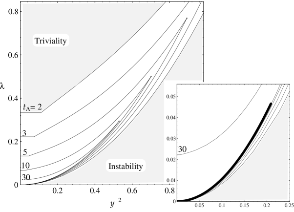
Figure 3: Regions in the $(\lambda_{0},y_{0}^{2})$ plane restricted by triviality and instability bounds. The reference scale $\mu_{0}$ of $t=\ln(\mu/\mu_{0})$ is fixed by $\alpha(t\!=\!0)=0.1$, and the parameters $N_{\rm C}=3,N_{\rm f}=6,n_{\rm f}=1$ and $R=\;$fundamental repr. are taken. The triviality bounds (upper lines) determined by $\lambda(t_{\Lambda})=\infty$ and the instability bounds by $\lambda(t_{\Lambda})=0$ are shown for $t_{\Lambda}=2,3,5,10,30$ and $\infty$. The allowed regions shrink to the line (3.23) as $t_{\Lambda}\rightarrow\infty$, which is drawn by the bold line in the enlarged figure in the bottom right. Again the running of $\lambda(t)$ is determined by using one-loop $\beta_{\lambda}(\lambda)$ of pure $\lambda\phi^{4}$ theory whenever the inequality $\lambda(t)\geq N_{\rm C}y^{2}(t)$ holds.

In the SM, this is related to the so-called “triviality bound” for the masses of Higgs boson and top quark[14]. What is special to the present case is that the allowed parameter region for $y^{2}_{0}$ and $\lambda_{0}$ shrinks to a line connecting the “Gaussian” and PR fixed points. Actually, in Fig. 3, we have also drawn “triviality bound” and “instability bound” on the $(y_{0}^{2},\lambda_{0})$ plane, which are determined by requiring $\lambda(t_{\Lambda})=\infty$ and $\lambda(t_{\Lambda})=0$, respectively, at a certain UV scale $t_{\Lambda}$. The theories with the parameters $(y_{0}^{2},\lambda_{0})$ inside the region enclosed by those two bounds give allowed cutoff theories possessing finite and positive couplings $y^{2}(t)$ and $\lambda(t)$ over the energy region $0\leq t<t_{\Lambda}$. As $t_{\Lambda}$ goes to infinity, this allowed parameter region is indeed seen to shrink to the line given by Eq. (3.23).

4 Renormalizability of Gauged NJL Model

We now turn to the discussion on the renormalizability of the gauged NJL model. The Lagrangian of the model is given by

$${\cal L}_{\rm GNJL}=-\frac{1}{4}\left(F_{\mu\nu}\right)^{2}+\sum_{i=1}^{N_{\rm f}}\overline{\psi_{i}}\,i\,\hbox to0.0pt{/\hss}\!D\psi_{i}+G\sum_{i=1}^{n_{\rm f}}\left(\overline{\psi_{i}}\psi_{i}\right)^{2}\ ,$$ (4.1)

where $G$ is a four-fermion coupling constant. For later convenience, we introduce a dimensionless coupling constant $g_{4}$ by

$$G\equiv\frac{(4\pi)^{2}}{a}\frac{g_{4}(\Lambda)}{\Lambda^{2}}\ ,$$ (4.2)

where $\Lambda$ is the UV cutoff.

As usual, we rewrite the four-fermion interaction by the standard method of introducing an auxiliary field. The resultant Lagrangian can be identified with that of a gauge-Higgs-Yukawa system under a suitable compositeness condition, which in particular requires[15] the vanishingness of the wave function renormalization factor, $Z_{\sigma}=0$, of the scalar field $\sigma$. According to Bardeen, Hill and Lindner[16], such compositeness condition can be stated most conveniently as a set of boundary conditions for the running parameters of the gauge-Higgs-Yukawa system at the compositeness scale $t_{\Lambda}\equiv\ln(\Lambda/\mu_{0})$, i.e., at the cutoff of the gauged NJL model. As for the dimensionless coupling constants[16], it reads

$$\frac{1}{y^{2}(t_{\Lambda})} = 0\ ,$$ (4.3)

$$\frac{\lambda(t_{\Lambda})}{y^{4}(t_{\Lambda})} = 0\ .$$ (4.4)

In addition to these, the compositeness condition gives a boundary condition for the mass parameter $m^{2}$ of $\sigma$, which relate $m^{2}(t_{\Lambda})$ to the four-fermion coupling constant $G$. There are, however, some subtleties in this condition for the mass parameter. So we defer the discussion to the next section.

Now, with the compositeness condition (4.3) and (4.4), we discuss the renormalizability of the gauged NJL model by utilizing the result in section 3 for the nontriviality of the gauge-Higgs-Yukawa system. We shall show in the next section that the mass parameter $m^{2}(t)$ can be made finite by the renormalization of the four-fermion coupling $G$. So we concentrate on the renormalization problem of the coupling constants $y^{2}$ and $\lambda$ here. The conditions (4.3) and (4.4) uniquely specify the RG flow corresponding to the gauged NJL model; by substituting them into Eqs. (2.9) and (2.10), the RG invariant constants $h_{0}$ and $k_{0}$ are determined in terms of gauge coupling constant at the cutoff scale as

$$h_{0} = -\eta^{c/b-1}(t_{\Lambda})=-\left(\frac{\alpha(t_{\Lambda})}{\alpha_{0}}\right)^{c/b-1}\ ,$$ (4.5)

$$k_{0} = -\eta^{2c/b-1}(t_{\Lambda})=-\left(\frac{\alpha(t_{\Lambda})}{\alpha_{0}}\right)^{2c/b-1}\ .$$ (4.6)

Then the Yukawa and quartic scalar couplings are given by

$$y^{2}(t) = \frac{c-b}{a}g^{2}(t)\left[1-\left(\frac{\alpha(t)}{\alpha(t_{\Lambda})}\right)^{1-c/b}\right]^{-1}\ \equiv\ y_{\Lambda}^{2}(t)\ ,\qquad\raisebox{-20.0pt}[0.0pt][0.0pt]{$\displaystyle(t<t_{\Lambda})$}$$ (4.7)

$$\frac{\lambda(t)}{y^{4}(t)} = \frac{2av}{2c-b}\frac{1}{g^{2}(t)}\left[1-\left(\frac{\alpha(t)}{\alpha(t_{\Lambda})}\right)^{1-2c/b}\right]\ \equiv\ \frac{\lambda_{\Lambda}(t)}{y_{\Lambda}^{4}(t)}\ .$$ (4.8)

The gauged NJL model with a cutoff $\Lambda$ is equivalent to the gauge-Higgs-Yukawa system with the same cutoff $\Lambda$ with the Yukawa and quartic scalar couplings given by Eqs. (4.7) and (4.8).

When we vary the cutoff $\Lambda$, the equivalent gauge-Higgs-Yukawa systems specified by Eqs. (4.5) and (4.6) define a sequence of theories parameterized by $\Lambda$. Now the question of the renormalizability of the gauged NJL model is whether the sequence converges in the $\Lambda\rightarrow\infty$ limit to a nontrivial theory. On the other hand, we know already that the gauge-Higgs-Yukawa system is nontrivial only when $h_{0}\geq 0$ and $k_{0}=0$. In view of the expressions (4.5) and (4.6), the only possibility is that

$$h_{0}\ ,\ k_{0}\ \longrightarrow\ -0\ .$$ (4.9)

This is realized only when $c>b$, which is just the condition for the nontriviality of gauge-Higgs-Yukawa system.

We therefore conclude that the gauged NJL model becomes renormalizable (without becoming trivial theory) if and only if its matter content satisfies $c>b$, and that the resultant continuum theory becomes identical with the gauge-Higgs-Yukawa system just on the PR fixed point, $h_{0}=k_{0}=0$. The resultant Yukawa and quartic scalar couplings are given by their fixed point values (3.1) and (3.2).

Note that the condition $c>b$ is automatically satisfied when we consider the fixed coupling limit $b\rightarrow+0$ since $c$ is a positive constant. It then follows that the gauged NJL model in this limit is always renormalizable. This agrees with KTY’s result for the fixed gauge coupling case.[1] The renormalized Yukawa and quartic scalar couplings (4.7) and (4.8) under the compositeness condition are found in the limit $b\rightarrow+0$ by using the formula (2.13) to reduce to

$$y_{\Lambda}^{2}(t) = \frac{(4\pi)^{2}}{2a}\frac{\alpha}{\alpha_{\rm c}}\left[1-\left(\frac{\mu}{\Lambda}\right)^{\alpha/\alpha_{\rm c}}\right]^{-1}\ \mathop{-\!\!\!-\!\!\!-\!\!\!-\!\!\!\!\!\longrightarrow}_{\Lambda\rightarrow\infty}\ \frac{(4\pi)^{2}}{2a}\frac{\alpha}{\alpha_{\rm c}}\equiv y^{2}_{\star}\ ,$$ (4.10)

$$\frac{\lambda_{\Lambda}(t)}{y_{\Lambda}^{4}(t)} = \frac{2av}{(4\pi)^{2}}\frac{\alpha_{\rm c}}{\alpha}\left[1-\left(\frac{\mu}{\Lambda}\right)^{2\alpha/\alpha_{\rm c}}\right]\ \ \ \mathop{-\!\!\!-\!\!\!-\!\!\!-\!\!\!\!\!\longrightarrow}_{\Lambda\rightarrow\infty}\ \frac{2av}{(4\pi)^{2}}\frac{\alpha_{\rm c}}{\alpha}\equiv\frac{\lambda_{\star}}{y^{4}_{\star}}\ ,$$ (4.11)

where $y^{2}_{\star}$ and $\lambda_{\star}$ denote the PR fixed point values.

We should note that the presence of gauge interaction is essential for this renormalizability. This is of course the consequence of the fact that nontrivial Higgs-Yukawa system can exist only in the presence of gauge interaction. Let us demonstrate this more directly in the NJL model by considering the limit of switching the gauge interaction off. By using Eq. (2.8), we take the limit $\alpha_{0}\rightarrow+0$ in Eqs. (4.7) and (4.8) and have

$$y^{2}_{\Lambda}(t) \!\!\!\!\!\!\mathop{-\!\!\!-\!\!\!-\!\!\!-\!\!\!\!\!\longrightarrow}_{\alpha_{0}\rightarrow+0}\ \frac{1}{2a}\frac{(4\pi)^{2}}{\ln(\Lambda/\mu)}\ \mathop{-\!\!\!-\!\!\!-\!\!\!-\!\!\!\!\!\longrightarrow}_{\Lambda\rightarrow\infty}\ 0\ ,$$ (4.12)

$$\lambda_{\Lambda}(t) \!\!\!\!\!\!\mathop{-\!\!\!-\!\!\!-\!\!\!-\!\!\!\!\!\longrightarrow}_{\alpha_{0}\rightarrow+0}\ \frac{\,v\,}{\,a\,}\frac{(4\pi)^{2}}{\ln(\Lambda/\mu)}\ \mathop{-\!\!\!-\!\!\!-\!\!\!-\!\!\!\!\!\longrightarrow}_{\Lambda\rightarrow\infty}\ 0\ .$$ (4.13)

We see that the renormalized couplings identically vanish in the continuum limit and that the NJL model is trivial and hence nonrenormalizable in the absence of gauge interaction.

5 Compositeness Condition for Mass Parameter

As mentioned in the preceding section, there are some subtleties in the compositeness condition for the mass parameter. This condition is important to see how the four-fermion coupling constant $G$ determines the phase structure of the equivalent gauge-Higgs-Yukawa system. It was argued in ref. [4] that the compositeness condition for the mass parameter is given by

$$\frac{1}{2}\frac{m_{\rm{\scriptscriptstyle MD}}^{2}(t_{\Lambda})}{y^{2}(t_{\Lambda})}=G^{-1}=\frac{a}{(4\pi)^{2}}\frac{\Lambda^{2}}{g_{4}(\Lambda)}\ ,$$ (5.1)

where $m_{\rm{\scriptscriptstyle MD}}$ is the mass parameter in the mass-dependent (MD) scheme. The mass parameter $m_{\rm{\scriptscriptstyle MD}}^{2}(t)$ renormalized at $t=\ln(\mu/\mu_{0})$ is related to $m^{2}(t)$ in the mass-independent $\overline{\rm MS}$ scheme to the leading order in our approximation as

$$m_{\rm{\scriptscriptstyle MD}}^{2}(t)=m^{2}(t)+\frac{2a}{(4\pi)^{2}}y^{2}(t)\mu^{2}\ ,$$ (5.2)

while other dimensionless coupling constants remain the same in both schemes. The RGE’s for these mass parameters are, respectively, given by

$$16\pi^{2}\frac{d}{dt}m^{2}(t) = 2a\,y^{2}(t)m^{2}(t)\ ,$$ (5.3)

$$16\pi^{2}\frac{d}{dt}m_{\rm{\scriptscriptstyle MD}}^{2}(t) = 2a\,y^{2}(t)\left[m_{\rm{\scriptscriptstyle MD}}^{2}(t)+2\mu^{2}\right]\ .$$ (5.4)

Since we are using the $\overline{\rm MS}$ renormalization scheme everywhere, we have to rewrite this compositeness condition (5.1) in terms of the mass parameter $m^{2}$ in the $\overline{\rm MS}$ scheme. If we use the relation (5.2) literally, the compositeness condition (5.1) is rewritten into

$$\frac{1}{2}\frac{m^{2}(t_{\Lambda})}{y^{2}(t_{\Lambda})}=\frac{a}{(4\pi)^{2}}\Lambda^{2}\left[\frac{1}{g_{4}(\Lambda)}-1\right]\ ,$$ (5.5)

which was shown in ref. [17] to work well, like the original one (5.1), to the leading order in $1/N_{\rm C}$ expansion in the Higgs-Yukawa system without gauge interaction.

In the presence of the gauge interaction, however, Eq. (5.5) is not correct since the leading-order relation (5.2) between the mass parameters in the $\overline{\rm MS}$ and MD schemes is not consistent with the RGE’s (5.3) and (5.4). Generally, such approximate relations like Eq. (5.2) between running parameters in two different renormalization schemes are not RG invariant and hence are valid only in a restricted region of renormalization points. Since the compositeness condition relates the low-energy parameters to those at the cutoff $\Lambda$, the naive use of the leading-order relation (5.2) is problematic.

For illustration, suppose that we calculate the effective potential in the $\lambda\phi^{4}$ theory to the leading-log order using two different renormalization schemes ${\cal R}_{1}$ and ${\cal R}_{2}$. Then we need to know one-loop $\beta$ functions and tree-level potential forms in both schemes[18]. The potentials in ${\cal R}_{1}$ and ${\cal R}_{2}$, in particular the coupling constants $\lambda_{1}(\mu)$ and $\lambda_{2}(\mu)$, are generally the same at the tree level. But the tree level relation $\lambda_{1}(\mu)=\lambda_{2}(\mu)$, for instance, is not invariant under one-loop RGE, and receives loop corrections of the form

$$\lambda_{1}(\mu)=\lambda_{2}(\mu)+a\frac{\lambda_{2}^{2}(\mu)}{(4\pi)^{2}}\ln\frac{m^{2}(\mu)}{\mu^{2}}+b\frac{\lambda_{2}^{3}(\mu)}{(4\pi)^{4}}\left(\ln\frac{m^{2}(\mu)}{\mu^{2}}\right)^{2}+\cdots\ .$$ (5.6)

We see from this that the RG non-invariant relation $\lambda_{1}(\mu)=\lambda_{2}(\mu)$ is valid only around $\mu^{2}\simeq m^{2}(\mu)$ where the loop corrections are small.

Our present leading-order relation (5.2) is not RG invariant in the presence of gauge interaction and is analogous to the above tree-level relation $\lambda_{1}(\mu)=\lambda_{2}(\mu)$. The gauge interaction effects appear from two-loop levels and give corrections to Eq. (5.2) in the form

$$m_{\rm{\scriptscriptstyle MD}}^{2}(t)=\left[m^{2}(t)+\frac{2a}{(4\pi)^{2}}y^{2}(t)\mu^{2}\right]+\mbox{(const.)}\times y^{2}(t)\alpha(t)\mu^{2}+\cdots\ .$$ (5.7)

From this, we understand that the leading-order relation (5.2) is most reliable at $\mu=0$ (or $t=-\infty$). In other words, the mass parameters in $\overline{\rm MS}$ and MD schemes should be identified with each other at $\mu=0$. Such identification at $\mu=0$ is all right for the fixed gauge-coupling case, but is problematic in the running gauge-coupling case since the running coupling $\alpha(t)$ in our approximation diverges at some finite $\mu=\Lambda_{\rm QCD}$ before reaching $\mu=0$. This implies that the relation between $\overline{\rm MS}$ and MD masses is in fact a very non-perturbative, dynamical problem with respect to the gauge interaction. This could be expected from the beginning if we recall the following facts: the $\overline{\rm MS}$ mass parameter $m^{2}(t)$ does not change sign under the change of the renormalization point $\mu$ since $m^{2}(t)$ is multiplicatively renormalized. But the sign of $m^{2}(t)$ determines whether the spontaneous breaking of the symmetry ($\sigma\rightarrow-\sigma$) occurs or not, and hence is a very dynamical quantity by itself. Moreover, if the asymptotically free gauge interaction is present, which becomes strong in the infrared region, we expect that the symmetry is always spontaneously broken just like the chiral symmetry in the actual QCD. If so, the $\overline{\rm MS}$ mass $m^{2}(t)$ should be sensitive to the presence of gauge interaction, in particular, to its infrared behavior.

However, we actually have no idea about how the ‘true’ running gauge-coupling $\alpha(t)$ behaves in the region $0\leq\mu\mathrel{\mathchoice{\vbox{\offinterlineskip\halign{$\m@th\displaystyle\hfil#\hfil$\cr<\crcr\sim\crcr} }}{\vbox{\offinterlineskip\halign{$\m@th\textstyle\hfil#\hfil$\cr<\crcr\sim\crcr} }}{\vbox{\offinterlineskip\halign{$\m@th\scriptstyle\hfil#\hfil$\cr<\crcr\sim\crcr} }}{\vbox{\offinterlineskip\halign{$\m@th\scriptscriptstyle\hfil#\hfil$\cr<\crcr\sim\crcr} }}}\Lambda_{\rm QCD}$. Therefore, we are obliged to choose a scale $\mu=\mu_{{\rm{\scriptscriptstyle C}}}$ at which we rely the leading-order relation (5.2) to be somewhere around $\Lambda_{\rm QCD}$ but a bit above it: we choose

$$\mu_{{\rm{\scriptscriptstyle C}}}=O(1)\times\Lambda_{\rm QCD}\ .$$ (5.8)

With this understanding, we improve the leading order relation (5.2) into a relation between RG invariant quantities. The RG invariant combination can easily be found in the $\overline{\rm MS}$ scheme: from the RGE (5.3) as well as the RGE’s (2.2) and (2.3), we find that the combination

$$\eta^{c/b}(t)\frac{m^{2}(t)}{y^{2}(t)}$$ (5.9)

is independent of $t=\ln(\mu/\mu_{0})$. The invariant in the MD scheme is a little bit harder to find. But we can obtain the following equation from the RGE (5.4):

$$\frac{d}{dt}\left[\eta^{c/b}(t)\frac{m_{\rm{\scriptscriptstyle MD}}^{2}(t)}{y^{2}(t)}\right] = \frac{2a}{(4\pi)^{2}}2\mu^{2}\eta^{c/b}(t)\ .$$ (5.10)

Integrating this equation from some arbitrary point $t_{{\rm{\scriptscriptstyle C}}}$ to $t$, we find a $t$-independent combination in the MD scheme:

$$\eta^{c/b}(t)\left[\frac{m_{\rm{\scriptscriptstyle MD}}^{2}(t)}{y^{2}(t)}-\frac{2a}{(4\pi)^{2}}\frac{\mu^{2}}{\Omega_{0}(t;t_{{\rm{\scriptscriptstyle C}}})}\right]\ ,$$ (5.11)

where $\Omega_{0}(t;t_{{\rm{\scriptscriptstyle C}}})$ is defined by an integral

$$\Omega_{0}^{-1}(t;t_{{\rm{\scriptscriptstyle C}}}) \equiv e^{-2t}\eta^{-c/b}(t)\int_{t_{{\rm{\scriptscriptstyle C}}}}^{t}2dze^{2z}\eta^{c/b}(z)\ .$$ (5.12)

Now that we have found the RG invariants both in the $\overline{\rm MS}$ and MD schemes, we can improve the leading-order relation (5.2) to the relation between the RG invariant quantities. Let us choose $t_{{\rm{\scriptscriptstyle C}}}\equiv\ln(\mu_{{\rm{\scriptscriptstyle C}}}/\mu_{0})$ to be a scale (5.8) at which the leading-order relation (5.2) is reliable:

$$\frac{m^{2}(t_{{\rm{\scriptscriptstyle C}}})}{y^{2}(t_{{\rm{\scriptscriptstyle C}}})}=\frac{m_{\rm{\scriptscriptstyle MD}}^{2}(t_{{\rm{\scriptscriptstyle C}}})}{y^{2}(t_{{\rm{\scriptscriptstyle C}}})}-\frac{2a}{(4\pi)^{2}}\mu_{{\rm{\scriptscriptstyle C}}}^{2}\ .$$ (5.13)

Then rewriting both sides of this equation by using the RG invariants (5.9) and (5.11), we have

$$\frac{m^{2}(t)}{y^{2}(t)}=\frac{m_{\rm{\scriptscriptstyle MD}}^{2}(t)}{y^{2}(t)}-\frac{2a}{(4\pi)^{2}}\frac{\mu^{2}}{\Omega(t;t_{{\rm{\scriptscriptstyle C}}})}\ ,$$ (5.14)

where $\Omega(t;t_{{\rm{\scriptscriptstyle C}}})$ is defined by

$$\Omega^{-1}(t;t_{{\rm{\scriptscriptstyle C}}}) \equiv \Omega_{0}^{-1}(t;t_{{\rm{\scriptscriptstyle C}}})+\left(\frac{\eta(t_{{\rm{\scriptscriptstyle C}}})}{\eta(t)}\right)^{c/b}\frac{\mu_{{\rm{\scriptscriptstyle C}}}^{2}}{\mu^{2}}$$ (5.15)

$$= 2e^{-2t}\alpha^{-c/b}(t)\left[\int_{t_{{\rm{\scriptscriptstyle C}}}}^{t}dze^{2z}\alpha^{c/b}(z)+\int_{-\infty}^{t_{{\rm{\scriptscriptstyle C}}}}dze^{2z}\;\alpha^{c/b}(t_{{\rm{\scriptscriptstyle C}}})\right]\ .$$ (5.16)

An important point is that while the original relation (5.2) does not include the gauge interaction corrections, this improved relation (5.14) does contain them in the RHS in the form of $\Omega^{-1}(t;t_{{\rm{\scriptscriptstyle C}}})$. It may be amusing to note that Eq. (5.16) looks like as if we are using as the running gauge coupling constant a cutoff form: $\theta(t-t_{{\rm{\scriptscriptstyle C}}})\alpha(t)+\theta(t_{{\rm{\scriptscriptstyle C}}}-t)\alpha(t_{{\rm{\scriptscriptstyle C}}})$.

Having the improved relation between the mass parameters in the $\overline{\rm MS}$ and MD schemes, we can now write down the compositeness condition which relates the mass parameter of the gauge-Higgs-Yukawa system to the four-fermion coupling constant of the gauged NJL model. Since the relation (5.14) holds at any scale $t$, we can now set $t$ equal to the cutoff $t_{\Lambda}=\ln(\Lambda/\mu_{0})$. Then, by substituting it into the compositeness condition (5.1), we obtain

$$\frac{m^{2}(t_{\Lambda})}{y^{2}(t_{\Lambda})}=\frac{2a}{(4\pi)^{2}}\Lambda^{2}\left[\frac{1}{g_{4}(\Lambda)}-\frac{1}{\Omega(t_{\Lambda};t_{{\rm{\scriptscriptstyle C}}})}\right]\ .$$ (5.17)

This is the final form of our compositeness condition for the mass parameter.

We can now show that the mass parameter $m^{2}(t)$ at a low energy point $t$ can be made finite when $\Lambda\rightarrow\infty$ by the renormalization of the four fermion coupling constant $g_{4}(\Lambda)$, as announced in the previous section. Using Eq. (5.17) and the RG invariance of the quantity (5.9), it immediately follows that

$$m^{2}(t) = \frac{2a}{(4\pi)^{2}}\,y^{2}(t)\,\left(\frac{\alpha(t_{\Lambda})}{\alpha(t)}\right)^{c/b}\;\Lambda^{2}\left[\frac{1}{g_{4}(\Lambda)}-\frac{1}{\Omega(t_{\Lambda};t_{{\rm{\scriptscriptstyle C}}})}\right]$$

$$= \frac{2(c-b)}{4\pi}\,\alpha(t)\,\left\{\left(\frac{\alpha(t_{\Lambda})}{\alpha(t)}\right)^{c/b}\,\Lambda^{2}\,\left[1-\left(\frac{\alpha(t_{\Lambda})}{\alpha(t)}\right)^{1-c/b}\right]^{-1}\left[\frac{1}{g_{4}(\Lambda)}-\frac{1}{\Omega(t_{\Lambda};t_{{\rm{\scriptscriptstyle C}}})}\right]\right\}\ ,$$

where Eq. (4.7) is used in going to the second expression. This tells us that we can keep the low energy mass parameter $m^{2}(t)$ finite and independent of $\Lambda$. Namely, as the cutoff $\Lambda$ goes to infinity, the four fermion coupling constant $g_{4}(\Lambda)$ should be adjusted such that the quantity in the curly bracket in the second expression remains $\Lambda$-independent. Therefore the renormalization of $g_{4}(\Lambda)$ is performed as

$$\left(\frac{\alpha(t_{\Lambda})}{\alpha(t)}\right)^{c/b}\,\left[1-\left(\frac{\alpha(t_{\Lambda})}{\alpha(t)}\right)^{1-c/b}\right]^{-1}\,\Lambda^{2}\,\left[\frac{1}{g_{4}(\Lambda)}-\frac{1}{\Omega(t_{\Lambda};t_{{\rm{\scriptscriptstyle C}}})}\right]=\mu^{2}\left[\frac{1}{g_{4R}(\mu)}-\frac{1}{g_{4R}^{\ast}}\right]\,,$$ (5.19)

so that we have a renormalized expression

$$m^{2}(t)=\frac{2(c-b)}{4\pi}\,\alpha(t)\,\mu^{2}\left[\frac{1}{g_{4R}(\mu)}-\frac{1}{g_{4R}^{\ast}}\right].$$ (5.20)

Here $g_{4R}^{\ast}$ is a finite constant whose value depends on the definition of $g_{4R}(\mu)$. This completes the renormalizability proof of the gauged NJL model discussed in the previous section.

Before closing this section, we consider the fixed gauge coupling limit for later convenience. As we discussed above, we can take $t_{{\rm{\scriptscriptstyle C}}}\rightarrow-\infty$ ($\mu_{{\rm{\scriptscriptstyle C}}}=0$) without any problems in this case, and $\Omega(t;t_{{\rm{\scriptscriptstyle C}}})$ defined by Eq. (5.15) then reduces to a $t$-independent constant:

$$\Omega(t;t_{{\rm{\scriptscriptstyle C}}})\,\,\,\mathop{-\!\!\!-\!\!\!-\!\!\!-\!\!\!-\!\!\!-\!\!\!-\!\!\!\!\longrightarrow}_{b\rightarrow 0,\,t_{{\rm{\scriptscriptstyle C}}}\rightarrow-\infty}\,\,\,\omega\equiv 1-\frac{1}{2}\frac{\alpha}{\alpha_{\rm c}}\ .$$ (5.21)

By taking the limit $b\rightarrow 0$ in Eq. (LABEL:compcond:mass:MI:improved:2), we obtain

$$m^{2}(t)=\frac{2a}{(4\pi)^{2}}\,\left(\frac{\Lambda^{2}}{\mu^{2}}\right)^{\omega}{y_{\Lambda}^{2}(t)}\,\mu^{2}\left[\frac{1}{g_{4}(\Lambda)}-\frac{1}{\omega}\right]\ ,$$ (5.22)

where $y_{\Lambda}(t)$ is the Yukawa coupling given in Eq. (4.10).

6 Effective Potential and
Renormalization of Gauged NJL Model

We have established the renormalizability of the gauged NJL model with $c>b$ and clarified how the continuum limit $\Lambda\rightarrow+\infty$ is taken. In this section, we calculate the effective potential of the “renormalizable” gauged NJL model and explicitly perform the renormalization. We then compare the result with the previous one obtained by Kondo, Tanabashi and Yamawaki (KTY) for the fixed gauge coupling case by solving the ladder SD equation[1].

Our strategy to obtain the effective potential of the gauged NJL model is to improve the potential of the gauge-Higgs-Yukawa system supplemented with the compositeness condition by using the RGE. We follow the procedure described in detail in ref. [18] and adopt the $\overline{\rm MS}$ renormalization scheme. We hereafter restrict ourselves to the fixed gauge-coupling case since there the comparison with the previous KTY’s result is possible and every calculation can be done explicitly.

Let us start with the effective potential of the gauge-Higgs-Yukawa system in the leading order of our approximation:

$$V_{0}(g,y,\lambda,\sigma,m^{2}\,;\mu)=\frac{1}{2}m^{2}\sigma^{2}+\frac{1}{4}\lambda\sigma^{4}-\frac{a}{(4\pi)^{2}}M_{{\rm F}}^{4}\left[\ln\frac{M_{{\rm F}}^{2}}{\mu^{2}}-\frac{3}{2}\right]\ .$$ (6.1)

We note that the scalar field $\sigma$ is the renormalized one with the condition that its kinetic term is normalized to be unity and we also introduce the fermion mass in the background $\sigma$ by

$$M_{{\rm F}}\equiv y\sigma\ .$$ (6.2)

The RG improvement of the effective potential is achieved by noting the fact that the effective potential should be RG invariant:

$$V\left(g,y,\lambda,\sigma,m^{2}\,;\mu\right)=V\left(\overline{g}(t),\overline{y}(t),\overline{\lambda}(t),\overline{\sigma}(t),\overline{m}^{2}(t)\,;e^{t}\mu\right)\ ,$$ (6.3)

where the barred quantities $\overline{g}(t)$, $\overline{y}(t)$, $\cdots$, are the renormalized parameters at the scale $e^{t}\mu$;

$$\overline{x}(t)=x(e^{t}\mu)\qquad\qquad\mbox{for}\qquad x=g,y,\lambda,m^{2},\sigma\ .$$ (6.4)

[Do not confuse, e.g., $\overline{g}(t)$ with $g(t)$ in the preceding sections which stands for $g(\mu)$.] The $t$-dependence of these barred parameters are determined by Eqs. (2.2)–(2.4), (5.3) and

$$16\pi^{2}\frac{d}{dt}\overline{\sigma}(t)=-a\overline{y}^{2}(t)\overline{\sigma}(t)$$ (6.5)

with the initial condition $\overline{x}(t\!=\!0)=x(\mu)$. Then as was shown in ref. [18], the RG improved potential $V$ is given as follows: first evaluate the running parameters at $t$ determined by

$$\overline{M}_{{\rm F}}(t)=e^{t}\mu$$ (6.6)

and then, insert them into the leading-order potential $V_{0}$. Namely,

$$V(g,y,\lambda,\sigma,m^{2}\,;\mu)$$

$$=\left.V_{0}\left(\overline{g}(t),\overline{y}(t),\overline{\lambda}(t),\overline{\sigma}(t),\overline{m}^{2}(t)\,;e^{t}\mu\right)\right|_{\overline{M}_{{\rm F}}(t)=e^{t}\mu}$$

$$=\left.\left[\frac{1}{2}\overline{m}^{2}(t)\overline{\sigma}^{2}(t)+\frac{1}{4}\overline{\lambda}(t)\overline{\sigma}^{4}(t)-\frac{a}{(4\pi)^{2}}\overline{M}_{{\rm F}}^{4}(t)\left(\ln\frac{\overline{M}_{{\rm F}}^{2}(t)}{e^{2t}\mu^{2}}-\frac{3}{2}\right)\right]\right|_{\overline{M}_{{\rm F}}(t)=e^{t}\mu}\ .$$ (6.7)

Note that the condition (6.6) for $t$ is just chosen such that the logarithmic term drops out.

In order to find the value of $t$ satisfying the condition (6.6) for the improvement, let us examine the RG evolution of the running fermion mass $\overline{M}_{{\rm F}}^{2}(t)=\overline{y}^{2}(t)\overline{\sigma}^{2}(t)$. From the RGE’s (2.2), (2.3) and (6.5), we find the combination $\left(\overline{\alpha}(t)/\overline{\alpha}(0)\right)^{-c/b}\overline{M}_{{\rm F}}^{2}(t)$ RG-invariant. In the present fixed gauge-coupling case, this reduces to $e^{(\alpha/\alpha_{\rm c})t}\overline{M}_{{\rm F}}^{2}(t)$ and hence we have

$$e^{(\alpha/\alpha_{\rm c})t}\overline{M}_{{\rm F}}^{2}(t)=\overline{M}_{{\rm F}}^{2}(t\!=\!0)=M_{{\rm F}}^{2}(\mu)\ .$$ (6.8)

Substituting the condition (6.6), this determines the desired $t$ as

$$e^{t}=\left(\frac{M_{{\rm F}}(\mu)}{\mu}\right)^{2/(2+\alpha/\alpha_{\rm c})}=\left(\frac{M_{{\rm F}}(\mu)}{\mu}\right)^{1/(2-\omega)}\ ,$$ (6.9)

where $\omega$ is defined in Eq. (5.21).

Substituting the above $t$ into Eq. (6.7), we obtain the RG improved effective potential of the gauge-Higgs-Yukawa system. With the compositeness condition imposed, it becomes the RG invariant effective potential of the gauged NJL model: noting that $\overline{m}^{2}(t)\overline{\sigma}^{2}(t)$ is $t$-independent by Eqs. (5.3) and (6.5), we find the quadratic part in $\overline{\sigma}$ in the potential (6.7) to give

$$V_{2} \equiv \left.\left[\frac{1}{2}\overline{m}^{2}(t)\overline{\sigma}^{2}(t)\right]\right|_{\overline{M}_{{\rm F}}(t)=e^{t}\mu}=\frac{1}{2}m^{2}(\mu)\sigma^{2}(\mu)$$ (6.10)

$$= \frac{1}{2}\frac{2a}{(4\pi)^{2}}y_{\Lambda}^{2}(\mu)\,\mu^{2}\,\left(\frac{\Lambda^{2}}{\mu^{2}}\right)^{\omega}\left[\frac{1}{g_{4}(\Lambda)}-\frac{1}{\omega}\right]\,\sigma^{2}(\mu)\ ,$$

where in the last step we have used Eq. (5.22) resultant from the compositeness condition for the mass parameter. We next recall Eq. (4.11) which resulted from the compositeness condition for the coupling constants: it now reads by Eq. (6.4)

$$\frac{\overline{\lambda}_{\Lambda}(t)}{\overline{y}_{\Lambda}^{4}(t)}=\frac{2av}{(4\pi)^{2}}\frac{\alpha_{\rm c}}{\alpha}\left[1-\left(\frac{e^{t}\mu}{\Lambda}\right)^{2\alpha/\alpha_{\rm c}}\right]\ .$$ (6.11)

Using this and Eq. (6.9), the quartic part in the potential (6.7) is evaluated as follows:

$$V_{4} \equiv \left.\left[\frac{1}{4}\frac{\overline{\lambda}(t)}{\overline{y}^{4}(t)}\overline{M}_{{\rm F}}^{4}(t)+\frac{3a}{2(4\pi)^{2}}\overline{M}_{{\rm F}}^{4}(t)\right]\right|_{\overline{M}_{{\rm F}}(t)=e^{t}\mu}$$ (6.12)

$$= \frac{2av}{4(4\pi)^{2}}\frac{\alpha_{\rm c}}{\alpha}\mu^{4}\left[\left(\frac{M_{{\rm F}}^{4}(\mu)}{\mu^{4}}\right)^{1/(2-\omega)}-\left(\frac{\mu^{2}}{\Lambda^{2}}\right)^{\alpha/\alpha_{\rm c}}\frac{M_{{\rm F}}^{4}(\mu)}{\mu^{4}}\right]$$

$$\qquad+\frac{3av}{2(4\pi)^{2}}\mu^{4}\left(\frac{M_{{\rm F}}^{4}(\mu)}{\mu^{4}}\right)^{1/(2-\omega)}\ ,$$

where $M_{{\rm F}}(\mu)=y_{\Lambda}(\mu)\sigma(\mu)$. Putting Eqs. (6.10) and (6.12) together, the potential (6.7) turns out to be

$$\frac{(4\pi)^{2}}{2a}\frac{V}{\mu^{4}} = \frac{1}{2}y_{\Lambda}^{2}(\mu)\left(\frac{\Lambda^{2}}{\mu^{2}}\right)^{\omega}\left[\frac{1}{g_{4}(\Lambda)}-\frac{1}{g_{4}^{\ast}}\right]\,\frac{\sigma^{2}(\mu)}{\mu^{2}}$$ (6.13)

$$\ {}+\frac{v}{4}\frac{\alpha_{\rm c}}{\alpha}\left[\left(\frac{y_{\Lambda}(\mu)\sigma(\mu)}{\mu}\right)^{4/(2-\omega)}-\left(\frac{\mu^{2}}{\Lambda^{2}}\right)^{\alpha/\alpha_{\rm c}}\left(\frac{y_{\Lambda}(\mu)\sigma(\mu)}{\mu}\right)^{4}\right]$$

$$\quad{}+\frac{3}{4}\left(\frac{y_{\Lambda}(\mu)\sigma(\mu)}{\mu}\right)^{4/(2-\omega)}\ ,$$

where

$$g_{4}^{\ast}\equiv\omega\ .$$ (6.14)

This is the desired RG-improved effective potential of the gauged NJL model with cutoff $\Lambda$. This potential $V$ satisfies the RGE and hence is independent of $\mu$.

We can now see explicitly how the effective potential is renormalized when the cutoff $\Lambda$ goes to infinity. As discussed in section 5, the quadratic term $V_{2}$ can be renormalized by the four-fermion coupling renormalization:

$$y_{\Lambda}^{2}(\mu)\left(\frac{\Lambda^{2}}{\mu^{2}}\right)^{\omega}\left[\frac{1}{g_{4}(\Lambda)}-\frac{1}{g_{4}^{\ast}}\right]=y^{2}_{\star}\left[\frac{1}{g_{4R}(\mu)}-\frac{1}{g_{4R}^{\ast}}\right]\ ,$$ (6.15)

where $y^{2}_{\star}$ denotes the PR fixed point value given by Eq. (4.10). There is still a term containing $\Lambda$ explicitly in Eq. (6.13), the last quartic term proportional to $(\mu^{2}/\Lambda^{2})^{\alpha/\alpha_{\rm c}}$, but it drops out as $\Lambda\rightarrow\infty$ since $\alpha/\alpha_{\rm c}>0$. We thus obtain the following finite expression

$$\frac{(4\pi)^{2}}{2a}\frac{V}{\mu^{4}}=\frac{1}{2}\left(\frac{1}{g_{4R}(\mu)}-\frac{1}{g_{4R}^{\ast}}\right)\frac{y^{2}_{\star}\sigma^{2}(\mu)}{\mu^{2}}+\frac{v}{4}\frac{\alpha_{\rm c}}{\alpha}\left(1+\frac{3}{v}\frac{\alpha}{\alpha_{\rm c}}\right)\left(\frac{y_{\star}\sigma(\mu)}{\mu}\right)^{4/(2-\omega)}\ ,$$ (6.16)

giving the final form of the renormalized effective potential in the gauged NJL model.

Some remarks are in order here. As we have discussed in section 4, the presence of gauge interaction is essential for the interaction term to exist nontrivially as in Eq. (6.16). Actually, if the gauge interaction is absent, we should take $\alpha\rightarrow 0$ in Eq. (6.13) before taking $\Lambda\rightarrow\infty$ limit and find

$$V = \frac{1}{2}\,\frac{1}{\ln(\Lambda/\mu)}\Lambda^{2}\left[\frac{1}{g_{4}(\Lambda)}-\frac{1}{g_{4}^{\ast}}\right]\,\sigma^{2}(\mu)$$ (6.17)

$${}+\frac{v}{4}\frac{(4\pi)^{2}}{2a}\left(\frac{1}{\ln(\Lambda/\mu)}\right)^{2}\left[2\ln(\Lambda/\mu)-\ln\left(\frac{(4\pi)^{2}}{2a}\frac{\sigma^{2}(\mu)}{\mu^{2}\ln(\Lambda/\mu)}\right)\right]\sigma^{4}(\mu)$$

$$\ {}+\frac{3}{4}\frac{(4\pi)^{2}}{2a}\left(\frac{1}{\ln(\Lambda/\mu)}\right)^{2}\sigma^{4}(\mu)\,.$$

The quadratic term can be made finite again by renormalizing $g_{4}(\Lambda)$ suitably, but the quartic term necessarily vanishes as $\Lambda\rightarrow\infty$, and this clearly shows the triviality of the pure NJL model. [The Yukawa term also vanishes as $(1/\ln(\Lambda/\mu))^{1/2}$. See Eq. (4.12).]

It may be interesting to see how this triviality is related with the usual knowledge of non-renormalizability of the NJL model. Recall that we have used the field variable $\sigma(\mu)$ which has a normalized kinetic term. If we had used the variable $\widetilde{\sigma}^{2}(\mu)\equiv\sigma^{2}(\mu)/\ln(\Lambda/\mu)\propto M_{{\rm F}}^{2}(\mu)$ and regarded it as finite ($\Lambda$-independent), then, we would obtain a finite Yukawa term, but would encounter logarithmic divergences in the scalar kinetic and quartic terms.

Our effective potential (6.13) and its renormalized version (6.16) should be compared with the previous results by Bardeen and Love[7] and by KTY[1], respectively, which were obtained by quite a different method using the SD equation in the ladder approximation. Our result takes precisely the same form as theirs under a suitable translation of notations: in particular our $\omega$, Eq. (5.21), is identified with KTY’s $\omega=\sqrt{1-\alpha/\alpha_{\rm c}}$. Both $\omega$ are of course the same in the first nontrivial order in the gauge coupling expansion in which we are working.

The potential (6.16) tells us the following: it is the sign of the coefficient of the quadratic term that determines whether the spontaneous breaking of the symmetry $(\sigma\rightarrow-\sigma)$ occurs or not. By Eq. (6.15), it is the same as the sign of $\left[1/g_{4}(\Lambda)-1/g_{4}^{\ast}\right]$. Therefore the critical value for the original four-fermion coupling constant $g_{4}(\Lambda)$ is given by $g_{4}^{\ast}=\omega$, Eq. (5.21). The critical coupling given by KTY was $(1+\omega)^{2}/4$ which also coincides with our result $\omega$ in the order $\alpha$ of the present approximation.

Finally, we can do the same calculations for the running gauge-coupling case also. There appears no essential difficulties, but the expression necessarily becomes implicit there since the value $t$ determined by Eq. (6.6) cannot be solved explicitly; it leads to, in place of (6.8),

$$\left(1+\frac{b\alpha_{0}}{2\pi}t\right)^{c/b}e^{2t}={M_{{\rm F}}^{2}(\mu)\over\mu^{2}}\ .$$ (6.18)

We here comment only on the critical four-fermion coupling constant, which can be given explicitly even in this running gauge-coupling case. The symmetry breaking is judged by the sign of the quadratic term $V_{2}$ in the effective potential $V$, which now reads, by using Eq. (LABEL:compcond:mass:MI:improved:2),

$$\!\!\!\!\!\!\!\!\!\!\!\frac{1}{2}\overline{m}^{2}(t)\overline{\sigma}^{2}(t) = \frac{1}{2}\frac{m^{2}(\mu)}{y^{2}(\mu)}M_{{\rm F}}^{2}(\mu)\ .$$ (6.19)

$$= \frac{1}{2}\frac{2a}{(4\pi)^{2}}\Lambda^{2}\left(1+\frac{b\alpha(\mu)}{2\pi}\ln\frac{\Lambda}{\mu}\right)^{-c/b}\left[\frac{1}{g_{4}(\Lambda)}-\frac{1}{\Omega(t_{\Lambda};t_{{\rm{\scriptscriptstyle C}}})}\right]M_{{\rm F}}^{2}(\mu)\ .$$

Therefore the critical coupling for $g_{4}(\Lambda)$ is given in this case by

$$g_{4}^{*}=\Omega(t_{\Lambda};t_{{\rm{\scriptscriptstyle C}}})\ .$$ (6.20)

If the cutoff is large enough such that $\Lambda\gg\mu_{{\rm{\scriptscriptstyle C}}}\simeq\Lambda_{\rm QCD}$ and $\alpha(\Lambda)\ll 1$,  this $\Omega(t_{\Lambda};t_{{\rm{\scriptscriptstyle C}}})$ is evaluated by Eq. (5.16) to be

$$\Omega^{-1}(t_{\Lambda};t_{{\rm{\scriptscriptstyle C}}})=1+\frac{\alpha(\Lambda)}{2\alpha_{\rm c}}+O\Big{(}\alpha^{2}(\Lambda),\ \frac{\mu_{{\rm{\scriptscriptstyle C}}}^{2}}{\Lambda^{2}}\Big{)}\ .$$ (6.21)

This again agrees with the previous result reported in Refs. [19, 8, 4].

7 Conclusions

We have explored in this paper the nontriviality constraint for the gauge-Higgs-Yukawa system and revealed the low-energy structure of the theory. The requirements of nontriviality and stability constrain the low energy Yukawa and quartic scalar couplings to lie on a line connecting “Gaussian” and the PR fixed points. The upper bound (the PR fixed point) can be apart from the “Gaussian” point only in the presence of gauge interaction.

The gauged NJL model is equivalent with the gauge-Higgs-Yukawa system supplemented by the compositeness condition. The equivalent gauge-Higgs-Yukawa theory with cutoff $\Lambda$ approaches the PR fixed point as $\Lambda\rightarrow\infty$ from outside the allowed region. Thus the continuum gauged NJL model lies on the boundary of the allowed region of the nontrivial gauge-Higgs-Yukawa system. This proves the renormalizability of gauged NJL model.

We have also calculated the effective potential of the gauged NJL model by using RGE. It is interesting that the result agrees with the KTY’s one which was obtained by quite a different method, the ladder SD equation.

In the model considered here, the scalar field was gauge-singlet. It may be interesting to investigate the case in which the gauge group is extended to a semi-simple one just like $SU(3)_{\rm C}\times SU(2)_{\rm L}$ in the SM, so that the scalar field becomes gauge-non-singlet. We expect that our main conclusions concerning the nontriviality and the renormalizability will remain true, but the coupling reduction of $\lambda$ to $y$ might no longer occur.

Note Added:

We are informed that Gusynin and Miransky [20] have derived a renormalized low-energy effective action in the broken phase of the gauged-NJL model (with fixed gauge coupling). See also the discussion for the symmetric phase at $\alpha\simeq\alpha_{\rm c}$ given in Miransky[21].

References

- [1] K.-I. Kondo, M. Tanabashi and K. Yamawaki, Prog. Theor. Phys. 89, 1249 (1993).
- [2] K.-I. Kondo, A. Shibata, M. Tanabashi and K. Yamawaki, Prog. Theor. Phys. 91, 541 (1994).
- [3] K.G. Wilson, Rev. Mod. Phys. 47, 773 (1975); K.G. Wilson and J. Kogut, Phys. Report 12C, 75 (1974); J. Polchinski, Nucl. Phys. B231, 269 (1984).
- [4] M. Bando, T. Kugo, N. Maekawa and H. Nakano, Phys. Rev. D44, R2957 (1991).
- [5] D.J.E. Callaway, Phys. Report 167, 241 (1988) and references therein.
- [6] B. Pendleton and G. Ross, Phys. Lett. 98B, 291 (1981).
- [7] W.A. Bardeen and S.T. Love, Phys. Rev. D45, 4672 (1992).
- [8] K.-I. Kondo, S. Shuto and K. Yamawaki, Mod. Phys. Lett. A6, 3385 (1991).
- [9] K. Yamawaki, in Proc. Workshop on Effective Field Theories of The Standard Model, Dobogókö, Hungary, Aug. 22-26, 1991, ed. U.-G. Meißner (World Scientific Pub. Co., Singapore, 1992); M. Tanabashi, in Proc. International Workshop on Electroweak Symmetry Breaking, Nov. 12-15, 1991, ed. W.A. Bardeen, J. Kodaira and T. Muta (World Scientific Pub. Co., Singapore, 1992).
- [10] N.V. Krasnikov, Mod. Phys. Lett. A8, 797 (1993).
- [11] J. Kubo, K. Sibold and W. Zimmermann, Phys. Lett. B220, 191 (1989).
- [12] N.-P. Chang, Phys. Rev. D10, 2706 (1974); E. Ma, Phys. Rev. D11, 322 (1975).
- [13] D. Gross and F. Wilczek, Phys. Rev. D8, 3633 (1973); T.P. Cheng, E. Eichten and L.-F. Li, Phys. Rev. D9, 2259 (1974).
- [14] N. Cabibbo, L. Maiani, G. Parisi and R. Petronzio, Nucl. Phys. B158, 295 (1979).
- [15] T. Eguchi, Phys. Rev. D17, 611 (1978); K. Shizuya, Phys. Rev. D21, 2327 (1980) and references cited therein.
- [16] W. Bardeen, C. Hill and M. Lindner, Phys. Rev. D41, 1647 (1990).
- [17] S. King and M. Suzuki, Phys. Lett. B277, 153 (1992).
- [18] M. Bando, T. Kugo, N. Maekawa and H. Nakano, Phys. Lett. B301, 83 (1993).
- [19] M. Bando, T. Kugo and K. Suehiro, Prog. Theor. Phys. 85, 1299 (1991).
- [20] V.P. Gusynin and V.A. Miransky, Mod. Phys. Lett. A6, 2443 (1991).
- [21] V.A. Miransky, Int. J. Mod. Phys. A8, 135 (1993).