SLAC-PUB-6525 hep-ph/9406286 June 1994 T/E

On the QCD corrections to $b\to s\gamma$ in supersymmetric models

Harald Anlauf

Stanford Linear Accelerator Center
Stanford University, Stanford, CA 94309

We reinvestigate the leading QCD corrections to the radiative decay $b\to s\gamma$ for supersymmetric extensions of the Standard Model. Although the major contributions to the corrections originate from the running of the effective Lagrangian from the W scale down to the $b$ scale, additional corrections are expected from large mass splittings between the particles running in the loops, as well as from integrating out heavy particles at scales different from the W mass. The calculation is performed in the framework of effective field theories.

Submitted to Nuclear Physics B

1 Introduction

Among the rare decays of B mesons, the recently observed radiative weak decays $\mathrm{B}\to X_{s}\gamma$ [1], where $X_{s}$ is a hadronic state with total strangeness $S=-1$, have received much attention. As a loop-induced FCNC process it is in particular sensitive to contributions from physics beyond the Standard Model (SM).

Since the $b$ quark mass is much larger than the QCD scale $\Lambda$, one assumes that the inclusive decay rate is well described by the spectator model, where the $b$ quark undergoes a radiative decay. The transition amplitude is given by the matrix element an effective magnetic moment operator. To lowest order [2], the coefficient of this operator is obtained by integrating out all heavy particles ($t$ quark, W boson, …), leaving one with an effective field theory describing the transition $b\to s\gamma$ at the parton level at the weak scale. The QCD corrections to this coefficient have been calculated to leading logarithmic accuracy in [4, 5, 6, 7, 8, 9] and are known to enhance the rate within the SM by a factor of 2–4, depending on the masses of the $b$ and of the $t$ quark. This enhancement is, however, subject to large uncertainties due to the poor knowledge of some input parameters like the strong coupling constant $\alpha_{S}$ and due to the residual renormalization scale dependence (for a recent discussion in the context of $b\to s\gamma$ see e.g. [10, 11, 12]), which we will however not address in this work.

On the other hand, if the particles in the loop have vastly different masses, one expects sizeable corrections to the Wilson coefficients already at the weak scale. These contributions, which are usually considered as a next-to-leading order effect, have been discussed in ref. [13] for the Standard Model where, in the case of a top quark much heavier than the W, they were found to give an additional enhancement of the order of 20%.

In the case of the Minimal Supersymmetric Standard Model (MSSM) [14], the situation is even more complicated. First of all, due to the richer particle content, there are more diagrams contributing to the magnetic moment operators, and due to the larger number of free parameters there are many potential additional sources of flavor changing neutral currents [15]. However, if one assumes further that the MSSM is a low energy effective theory from minimal supergravity [16] with radiative breaking of the electroweak symmetry, it is known [17, 11, 18, 19, 20, 21, 22, 23, 24, 25] that, besides the SM contribution mediated by the W, there are only significant contributions from the charged Higgs (${\mathrm{H}^{\pm}}$) and from the chargino ($\chi^{+}_{1,2}$) exchange diagrams, while already with the present experimental lower limits on the supersymmetry (SUSY) spectrum the gluino contribution is small and the neutralino contribution is always negligible. The W and the ${\mathrm{H}^{\pm}}$ contributions always have the same sign in the MSSM, but the chargino contribution can have either sign and may e.g. cancel the ${\mathrm{H}^{\pm}}$ contribution or (for small chargino masses and large $\tan\beta$) even dominate the amplitude.

Since SUSY has to be broken, the mass splitting between the various particles running in the loop can be very large, leading to additional important QCD corrections. We will advocate that, in a parameter space analysis in the MSSM, one should not simply add up the contributions of all diagrams at the W scale and use the renormalization group evolution to run down this sum to the $b$ scale, but rather consider the individual contributions separately. This is especially important for the chargino contribution, since the lightest chargino can be significantly lighter than the W.

For the reasons mentioned above, we will ignore the contributions from diagrams with gluinos and neutralinos in the present work. They may easily be included; corrections of the type considered in this work will however always be numerically unimportant.

Our strategy will be similar to the work by Cho and Grinstein [13]. Starting from the full theory at sufficiently high scales, we will construct a series of effective theories that is well suited for the description of the low-energy physics of interest. We shall give all ingredients that are necessary to obtain the leading QCD corrections to the $b\to s\gamma$ inclusive rate and discuss some simple estimates for an MSSM scenario with the assumptions mentioned above. A full parameter space analysis, which depends on the details of the implementation of the soft SUSY-breaking, is however beyond the scope of the present paper and will be discussed elsewhere.

This paper is organized as follows: In section 2 we briefly review the elements of effective field theories needed for the present work. Section 3 explains in detail the calculation for a type-II two-Higgs doublet model, which is contained in the MSSM, while the contributions of SUSY particles are discussed in section 4. We shall present our results in section 5 and finally conclude.

2 Effective field theory and $b\to s\gamma$

The basic idea of effective field theories is by now well established, and many excellent reviews have appeared in the literature [27, 28, 29, 30, 31]. Starting from some underlying full theory, one integrates out the heavy degrees of freedom, thereby producing a tower of non-renormalizable interactions (with couplings proportional to inverse powers of the heavy particle mass) which contain the virtual heavy particle effects. One then runs the resulting effective field theory down to the appropriate scale of interest using the renormalization group. If additional heavy particle thresholds are crossed during the renormalization group running, then these particles will also be integrated out. The major advantages of using an effective theory for the calculation of low-energy observables are convenience, since calculations are usually simpler than in the full theory, and the gain of insight.

A nontrivial feature of the effective field theory framework is the automatic summation of large logarithms that originate from perturbatively calculable short-distance physics by the renormalization group. As explained in detail e.g. in [31], the renormalization scale $\mu$ in a dimensional scheme (e.g. $\overline{\mathrm{MS}}$) serves to separate short-distance from long-distance physics. The Appelquist–Carazzone decoupling theorem [32] can be implemented properly in the (mass-independent) $\overline{\mathrm{MS}}$ scheme by hand by matching the effective theories below and above thresholds. The advantage of having a mass-independent scheme is that the renormalization group $\beta$-functions do not explicitly depend on the scale $\mu$, while the validity of the decoupling theorem guarantees that all intuitive reasoning based on a so-called physical renormalization scheme remains still true.

When the effective theory contains two heavy mass scales $m_{1},m_{2}$ of comparable magnitude, it is usually a good approximation to integrate out both particles at a common scale. On the other side, if the ratio $x\equiv(m_{1}/m_{2})^{2}$ is very small (i.e. $x\ll 1$), even if the coupling constant is small, the product $\alpha\ln x$ may become of order unity, and one is then forced to sum all powers of this product, while corrections to the sum are suppressed by powers of $\alpha$ or $x$. Sometimes the situation is less favorable and lies somewhere in between, as is the case e.g. for the SM with a heavy top quark [13] of, say, 175 GeV. For the process $b\to s\gamma$, the most important correction is the QCD running between the W and the $b$ scale, whose size is (parametrically) given by

$$\alpha_{S}(m_{\mathrm{W}})\cdot\ln(m_{\mathrm{W}}/m_{\mathrm{b}})^{2}\simeq 0.7\,,$$

while

$$\alpha_{S}(m_{\mathrm{W}})\cdot\ln(m_{\mathrm{t}}/m_{\mathrm{W}})^{2}\simeq(m_{\mathrm{W}}/m_{\mathrm{t}})^{2}\simeq 0.2$$

indicates that one might miss numerically important pieces if either of the latter would be neglected; compared to next-to-leading order corrections which are of order $\alpha_{S}\simeq 0.1$. What one can achieve with reasonable effort is to take into account the resummation of the leading terms in the limit of a heavy top quark, and then simply adding in the nonleading terms, thus neglecting terms which are (up to logarithms) $O(\alpha(m_{\mathrm{W}}/m_{\mathrm{t}})^{2})$. The choice of scale where to add these nonleading terms is at this stage completely arbitrary and can only be answered by a calculation of the power corrections. The remaining uncertainty is, however, less important than neglected next-to-leading order corrections.

Let us now turn to the application to the $b\to s\gamma$ transition. The effective Hamiltonian of interest may be written as a sum of $\Delta B=1$, $\Delta S=1$ operators:

$$H_{\mathrm{eff}}=\frac{4G_{\mathrm{F}}}{\sqrt{2}}K_{\mathrm{tb}}K_{\mathrm{ts}}^{*}\sum_{i}C_{i}(\mu){\cal O}_{i}(\mu)$$ (1)

A suitable operator basis $\{{\cal O}_{i}\}$ will be given below.

In general the definition of the operators in (1) will require the specification of a renormalization scheme. From the fact that the effective Hamiltonian is independent of the renormalization scale, one derives renormalization group equations for the composite operators ${\cal O}_{i}(\mu)$ and the coefficient functions $C_{i}(\mu)$. The renormalization of a composite operator is formally defined in terms of the divergent renormalization constants $Z_{ij}$ which relate renormalized and bare operators:

$${\cal O}_{i}^{\rm bare}=Z_{ij}(\mu){\cal O}_{j}(\mu)$$ (2)

Since the bare operators are $\mu$-independent, the renormalized operators depend on the subtraction scale via the $\mu$ dependence of the $Z_{ij}$:

$$\mu\frac{d}{d\mu}{\cal O}_{i}=\left(\mu\frac{d}{d\mu}Z^{-1}_{ij}\right){\cal O}_{j}^{\rm bare}=-\gamma_{ik}{\cal O}_{k},$$ (3)

where

$$\gamma_{ik}=Z^{-1}_{ij}\mu\frac{d}{d\mu}Z_{jk}$$ (4)

is the so called anomalous dimension matrix.

From the scale independence of the effective Hamiltonian (1) one derives the renormalization group equations for the Wilson coefficients $C_{i}$:

$$\mu\frac{d}{d\mu}C_{i}(\mu)=\sum_{j}\left(\gamma^{T}\right)_{ij}C_{j}(\mu)$$ (5)

If QCD corrections are neglected, the solution to this differential equation is straightforward. When QCD corrections are included, it turns out to be favorable to eliminate the derivative with respect to the renormalization scale in favor of a derivative with respect to the coupling constant:

$$\beta\frac{dC_{i}}{dg_{3}}=\sum_{j}\left(\gamma^{T}\right)_{ij}C_{j}$$ (6)

Here (and in the following) $g_{3}$ denotes the QCD coupling constant, and $\beta=\mu(dg_{3}/d\mu)$ is the QCD beta function.

The solution to the differential equation (6) is then given by

$$C(\mu)=T_{g}\left[\exp\int\limits_{g_{3}(\mu_{0})}^{g_{3}(\mu)}dg\,\frac{\gamma^{T}(g)}{\beta(g)}\right]C(\mu_{0}),$$ (7)

where $T_{g}$ means an ordering in the coupling such that $g$ increases from right to left (for $\mu<\mu_{0}$). Since our anomalous dimension matrices will be $g_{3}^{2}$ times a purely numerical matrix,

$$\gamma=\frac{g_{3}^{2}}{8\pi^{2}}\hat{\gamma}+O(g_{3}^{4})$$

the $g$-ordering is superfluous, and the $g$-integration is trivial:

$$C(\mu)=\exp\left[\left(\frac{1}{2b}\ln\frac{\alpha_{3}(\mu)}{\alpha_{3}(\mu_{0})}\right)\hat{\gamma}^{T}\right]C(\mu_{0})$$ (8)

The most convenient way to calculate the anomalous dimension matrix $\gamma$ is to consider Green functions with insertions of composite operators. Denote by $\Gamma^{(n)}_{{\cal O}_{i}}$ a renormalized $n$-point 1PI Green function with one insertion of the operator ${\cal O}_{i}$. The anomalous dimension $\gamma_{ij}$ that determines the mixing of ${\cal O}_{i}$ into ${\cal O}_{j}$ may then be simply read off from the renormalization group equation for $\Gamma^{(n)}_{{\cal O}_{i}}$,

$$\gamma_{ij}\Gamma^{(n)}_{{\cal O}_{j}}=-\left(\mu\frac{\partial}{\partial\mu}+\beta\frac{\partial}{\partial g}+\gamma_{m}m\frac{\partial}{\partial m}-n\gamma_{ext}\right)\Gamma^{(n)}_{{\cal O}_{i}}$$ (9)

Here $\gamma_{m}=(\mu/m)(dm/d\mu)$, and $n\gamma_{\rm ext}$ accounts for the wave-function anomalous dimensions arising from radiative corrections to the external lines of the Green functions.

We shall use dimensional regularization with minimal subtraction ($\overline{\mathrm{MS}}$), $d=4-2\epsilon$. The $\mathrm{SU}(3)_{\mathrm{C}}\times\mathrm{U}(1)_{\mathrm{em}}$ covariant derivative then reads:

$$D_{\mu}=\partial_{\mu}-i\mu^{\epsilon}g_{3}G^{a}_{\mu}X^{a}-i\mu^{\epsilon}eA_{\mu}Q$$ (10)

We will use the background field $R_{\xi}$ gauge [33] throughout this work. The anomalous dimensions of the fields are in this case given by:

$$\gamma_{\mathrm{quark}}=\frac{2}{3}\frac{g_{3}^{2}}{8\pi^{2}},\quad\gamma_{\mathrm{squark}}=-\frac{4}{3}\frac{g_{3}^{2}}{8\pi^{2}},\quad\gamma_{\mathrm{gluon}}=\frac{\beta}{g_{3}},$$

$$\gamma_{\mathrm{m}}=-4\frac{g_{3}^{2}}{8\pi^{2}},\quad\;\gamma_{\tilde{\mathrm{m}}}=-6\frac{g_{3}^{2}}{8\pi^{2}},\qquad\beta=b\frac{g_{3}^{3}}{8\pi^{2}}.$$ (11)

The coefficient appearing in the $\beta$-function has the value

$$b=-\frac{11}{2}+\frac{1}{3}n_{f}+\frac{1}{12}n_{\tilde{q}}+n_{\tilde{g}},$$ (12)

where $n_{f},n_{\tilde{q}}$ and $n_{\tilde{g}}$ are the number of active quark flavors, squarks and gluinos, respectively.

In all cases considered below, the operator basis of choice will contain the following set of operators involving only light degrees of freedom (i.e. photons, gluons, and “light” quarks with masses below $m_{\mathrm{W}}$):

Dimension $$d+1$$:

$${O_{\mathrm{LR}}^{1}} = -\frac{1}{16\pi^{2}}m_{\mathrm{b}}\bar{s}_{\mathrm{L}}D^{2}b_{\mathrm{R}}$$

$${O_{\mathrm{LR}}^{2}} = \mu^{\epsilon}\frac{g_{3}}{16\pi^{2}}m_{\mathrm{b}}\bar{s}_{\mathrm{L}}\sigma^{\mu\nu}X^{a}b_{\mathrm{R}}\;G^{a}_{\mu\nu}$$

$${O_{\mathrm{LR}}^{3}} = \mu^{\epsilon}\frac{eQ_{\mathrm{b}}}{16\pi^{2}}m_{\mathrm{b}}\bar{s}_{\mathrm{L}}\sigma^{\mu\nu}b_{\mathrm{R}}\;F_{\mu\nu}$$

Dimension $$d+2$$:

$$P^{1,A}_{\mathrm{L}} = -\frac{i}{16\pi^{2}}\bar{s}_{\mathrm{L}}T^{A}_{\mu\nu\sigma}D^{\mu}D^{\nu}D^{\sigma}b_{\mathrm{L}}$$

$${P_{\mathrm{L}}^{2}} = \mu^{\epsilon}\frac{eQ_{\mathrm{b}}}{16\pi^{2}}\bar{s}_{\mathrm{L}}\gamma^{\mu}b_{\mathrm{L}}\;\partial^{\nu}F_{\mu\nu}$$

$${P_{\mathrm{L}}^{4}} = i\mu^{\epsilon}\frac{eQ_{\mathrm{b}}}{16\pi^{2}}\bar{s}_{\mathrm{L}}\gamma^{\mu}\gamma^{5}D^{\nu}b_{\mathrm{L}}\;\tilde{F}_{\mu\nu}$$ (13)

The tensors $T^{A}_{\mu\nu\sigma}$ appearing in $P_{\mathrm{L}}^{1,A}$, $A=1,\ldots 4$, are defined by:

$$T^{1}_{\mu\nu\sigma}=g_{\mu\nu}\gamma_{\sigma}, T^{2}_{\mu\nu\sigma}=g_{\mu\sigma}\gamma_{\nu},$$

$$T^{3}_{\mu\nu\sigma}=g_{\nu\sigma}\gamma_{\mu}, T^{4}_{\mu\nu\sigma}=-i\epsilon_{\mu\nu\sigma\tau}\gamma^{\tau}\gamma_{5}$$ (14)

In order to apply the procedure outlined above to the MSSM case, we will consider in a first step the extension of the calculation by Cho and Grinstein [13] to the case of a type-II two-Higgs doublet model. There are already two cases to consider, namely that the charged Higgs can be either much lighter or much heavier than the $t$ quark. We shall then explain in detail how one adds to this picture the contributions induced by the chargino loops.

3 Two-Higgs doublet model

3.1 $m_{\mathrm{t}}>m_{\mathrm{H}^{\pm}}$

If the top quark is heavier than the W and the charged Higgs, then the first step is to integrate out the top quark at the scale $\mu=m_{\mathrm{t}}$. This leads to an effective field theory for $\mu<m_{\mathrm{t}}$ without the $t$, but with new vertices of dimension larger than four that contain the virtual $t$ effects. For the process under consideration, we need, in addition to the operator basis (2), further operators.

In general, in the range $m_{\mathrm{t}}>\mu>m_{\mathrm{W}}$, one has to consider higher dimensional operators which contain the W’s, the would-be Goldstone bosons $\phi_{\pm}$ and the charged Higgs field. By naive dimensional analysis, we expect that higher dimensional operators are suppressed by inverse powers of the ratio $x_{\mathrm{tW}}\equiv(m_{\mathrm{t}}/m_{\mathrm{W}})^{2}$. Since this ratio is not very large for phenomenologically acceptable top quark masses, the effects of the higher dimensional operators are not necessarily small, compared to the leading dimension 5 and dimension 6 operators. Also, the matching conditions at threshold in general are combinations of rational functions and polynomials in $x_{\mathrm{tW}}$.

Nevertheless, we shall take the approach motivated in the previous chapter and keep only the leading operators and the leading terms in the matching contributions. Although we are unable to calculate the power corrections, we shall later add the subleading terms in $1/x_{\mathrm{tW}}$, so that we get the same result in the limit of neglecting strong corrections for $\mu>m_{\mathrm{W}}$, as when all heavy particles are integrated out simultaneously at the W scale.

The relevant part of the interaction Lagrangian in the charged current sector reads

$$L_{\mathrm{CC}} = \frac{g_{2}}{\sqrt{2}}\,W^{+}_{\mu}\,\bar{U}\gamma^{\mu}KP_{\mathrm{L}}D+\mathrm{h.c.}$$

$$+ \frac{g_{2}}{\sqrt{2}m_{\mathrm{W}}}\left(\phi_{+}\bar{U}\left[M_{U}KP_{\mathrm{L}}-KM_{D}P_{\mathrm{R}}\right]D+\mathrm{h.c.}\right)$$

where $U=(u,c,t)$ and $D=(d,s,b)$ represent up-type and down-type quarks, respectively, $M_{U}=\mathrm{diag}(m_{\mathrm{u}},m_{\mathrm{c}},m_{\mathrm{t}})$, $M_{D}=\mathrm{diag}(m_{\mathrm{d}},m_{\mathrm{s}},m_{\mathrm{b}})$ are the quark mass matrices, $g_{2}=e/\sin\theta_{\mathrm{W}}$ is the gauge coupling of SU(2)_W, $P_{\mathrm{L},\mathrm{R}}$ are projectors on the left- and right-handed components of the fermions, and $K$ is the Kobayashi-Maskawa matrix. In the present work, we shall neglect the masses of the quarks of the first two generations whenever appropriate.

From these expression one can see that the leading terms for $x_{\mathrm{tW}}\gg 1$ come from vertices which involve the charged would-be Goldstone bosons $\phi_{\pm}$ and the top quark, since they are proportional to the top quark mass. For this reason, in the range $m_{\mathrm{t}}>\mu>m_{\mathrm{W}}$, we shall need, analogous to the findings in [13], the following operators with external would-be Goldstone bosons, in addition to the operator basis (2):

$$Q_{\mathrm{LR}} = \mu^{2\epsilon}\frac{g_{3}^{2}}{16\pi^{2}}m_{\mathrm{b}}\phi_{+}\phi_{-}\,\bar{s}_{\mathrm{L}}b_{\mathrm{R}}$$

$${R_{\mathrm{L}}^{1}} = i\mu^{2\epsilon}\frac{g_{3}^{2}}{16\pi^{2}}\phi_{+}\phi_{-}\,\bar{s}_{\mathrm{L}}D\hskip-6.49994pt/\,b_{\mathrm{R}}$$

$${R_{\mathrm{L}}^{2}} = i\mu^{2\epsilon}\frac{g_{3}^{2}}{16\pi^{2}}(D^{\mu}\phi_{+})\phi_{-}\,\bar{s}_{\mathrm{L}}\gamma_{\mu}b_{\mathrm{R}}$$ (16)

$${R_{\mathrm{L}}^{3}} = i\mu^{2\epsilon}\frac{g_{3}^{2}}{16\pi^{2}}\phi_{+}(D^{\mu}\phi_{-})\bar{s}_{\mathrm{L}}\gamma_{\mu}b_{\mathrm{R}}$$

The inclusion of explicit factors $g_{3}^{2}$ into these operators is motivated by the Gilman-Wise trick [34], which allows us to have all one-loop contributions to the anomalous dimension matrices to be of $O(g_{3}^{2})$, so that the diagonalization of these matrices is scale independent. We will freely use this trick later on.

The interaction Lagrangian for the charged Higgs with the quarks reads:

$$L_{{\mathrm{H}^{\pm}}f\bar{f}^{\prime}}=\frac{g_{2}}{\sqrt{2}m_{\mathrm{W}}}\left(H^{+}\bar{U}\left[\cot\beta M_{U}KP_{\mathrm{L}}+\tan\beta KM_{D}P_{\mathrm{R}}\right]D+\mathrm{h.c.}\right),$$ (17)

with $\tan\beta=v_{1}/v_{2}$ being the ratio of the vacuum expectation values of the Higgs fields which give rise to the masses of up- and down-type quarks, respectively.

The interaction (17) has the same structure and quark mass dependence of the couplings as the interaction of the would-be Goldstone bosons $\phi_{\pm}$, see (3.1). In the limit $x_{\mathrm{tH}}\equiv(m_{\mathrm{t}}/m_{\mathrm{H}^{\pm}})^{2}\gg 1$, keeping only the leading terms in $1/x_{\mathrm{tH}}$, we are lead to the following operators with charged Higgs bosons we have to add to our operator basis in the range $m_{\mathrm{t}}>\mu>m_{\mathrm{H}^{\pm}}$:

$$Q_{\mathrm{LR}}^{\prime} = \mu^{2\epsilon}\frac{g_{3}^{2}}{16\pi^{2}}m_{\mathrm{b}}H^{+}H^{-}\,\bar{s}_{\mathrm{L}}b_{\mathrm{R}}$$

$${R_{\mathrm{L}}^{1}}^{\prime} = i\mu^{2\epsilon}\frac{g_{3}^{2}}{16\pi^{2}}H^{+}H^{-}\,\bar{s}_{\mathrm{L}}D\hskip-6.49994pt/\,b_{\mathrm{R}}$$

$${R_{\mathrm{L}}^{2}}^{\prime} = i\mu^{2\epsilon}\frac{g_{3}^{2}}{16\pi^{2}}(D^{\mu}H^{+})H^{-}\,\bar{s}_{\mathrm{L}}\gamma_{\mu}b_{\mathrm{R}}$$ (18)

$${R_{\mathrm{L}}^{3}}^{\prime} = i\mu^{2\epsilon}\frac{g_{3}^{2}}{16\pi^{2}}H^{+}(D^{\mu}H^{-})\bar{s}_{\mathrm{L}}\gamma_{\mu}b_{\mathrm{R}}$$

3.1.1 Matching at $\mu=m_{\mathrm{t}}$

For $\mu>m_{\mathrm{t}}$, our effective theory is a fully renormalizable theory, which still contains all particles and interactions, so in this case all coefficients of our effective Hamiltonian are zero:

$$C_{i}(\mu=m_{\mathrm{t}}^{+})=0\qquad\mbox{for all $i$}$$ (19)

When we cross the $t$ threshold from above, i.e. when we integrate out the top quark at $\mu=m_{\mathrm{t}}$, we obtain the following changes to the coefficients of the effective Hamiltonian, due the interactions from the would-be Goldstone bosons from matching the three-point functions $\Gamma^{bs\gamma}$ and $\Gamma^{bsg}$ [13] (here $\Delta C_{i}=C_{i}(m_{\mathrm{t}}^{-})-C_{i}(m_{\mathrm{t}}^{+})$):

$$\Delta_{(\phi,W)}C_{{O_{\mathrm{LR}}^{1}}} = -\frac{1}{2}$$

$$\Delta_{(\phi,W)}C_{{O_{\mathrm{LR}}^{2}}} = \frac{Q_{\mathrm{b}}}{Q_{\mathrm{t}}}\Delta_{(\phi,W)}C_{{O_{\mathrm{LR}}^{3}}}=-\frac{1}{2}$$

$$\Delta_{(\phi,W)}C_{{P^{1,1}_{\mathrm{L}}}} = \Delta_{(\phi,W)}C_{{P^{1,3}_{\mathrm{L}}}}=\frac{11}{18}$$

$$\Delta_{(\phi,W)}C_{{P^{1,2}_{\mathrm{L}}}} = -\frac{8}{9}$$

$$\Delta_{(\phi,W)}C_{{P^{1,4}_{\mathrm{L}}}} = -Q_{\mathrm{b}}\Delta_{(\phi,W)}C_{{P_{\mathrm{L}}^{4}}}=\frac{1}{2}$$

$$\Delta_{(\phi,W)}C_{{P_{\mathrm{L}}^{2}}} = \frac{3}{4Q_{\mathrm{b}}}$$

$$\Delta_{(\phi,W)}C_{Q_{\mathrm{LR}}} = -\frac{16\pi^{2}}{g_{3}^{2}}$$

$$\Delta_{(\phi,W)}C_{{R_{\mathrm{L}}^{1}}} = \Delta_{(\phi,W)}C_{{R_{\mathrm{L}}^{2}}}=\frac{16\pi^{2}}{g_{3}^{2}}$$

$$\Delta_{(\phi,W)}C_{{R_{\mathrm{L}}^{3}}} = 0$$ (20)

Similarly, there are contributions from the interactions with the charged Higgs bosons:

$$\Delta_{(H)}C_{{O_{\mathrm{LR}}^{1}}} = \frac{1}{2}$$

$$\Delta_{(H)}C_{{O_{\mathrm{LR}}^{2}}} = \frac{Q_{\mathrm{b}}}{Q_{\mathrm{t}}}\Delta_{(H)}C_{{O_{\mathrm{LR}}^{3}}}=\frac{1}{2}$$

$$\Delta_{(H)}C_{{P^{1,1}_{\mathrm{L}}}} = \Delta_{(H)}C_{{P^{1,3}_{\mathrm{L}}}}=\frac{11}{18}\cot^{2}\beta$$

$$\Delta_{(H)}C_{{P^{1,2}_{\mathrm{L}}}} = -\frac{8}{9}\cot^{2}\beta$$

$$\Delta_{(H)}C_{{P^{1,4}_{\mathrm{L}}}} = -Q_{\mathrm{b}}\Delta_{(H)}C_{{P_{\mathrm{L}}^{4}}}=\frac{1}{2}\cot^{2}\beta$$

$$\Delta_{(H)}C_{{P_{\mathrm{L}}^{2}}} = \frac{3}{4Q_{\mathrm{b}}}\cot^{2}\beta$$

$$\Delta_{(H)}C_{Q_{\mathrm{LR}}^{\prime}} = \frac{16\pi^{2}}{g_{3}^{2}}$$

$$\Delta_{(H)}C_{{R_{\mathrm{L}}^{1}}^{\prime}} = \Delta_{(H)}C_{{R_{\mathrm{L}}^{2}}^{\prime}}=\frac{16\pi^{2}}{g_{3}^{2}}\cot^{2}\beta$$

$$\Delta_{(H)}C_{{R_{\mathrm{L}}^{3}}^{\prime}} = 0$$ (21)

At this point it is worthwhile to note that, had we not matched at the scale $\mu=m_{\mathrm{t}}$ but at a different scale (or used a different subtraction scheme), we would have found logarithmic contributions in the matching corrections to the coefficient of ${P_{\mathrm{L}}^{2}}$:

$$\Delta_{(\phi,W)}C_{{P_{\mathrm{L}}^{2}}}=\frac{1}{Q_{\mathrm{b}}}\left[\frac{3}{4}+\frac{1}{6}\ln\frac{\mu^{2}}{m_{\mathrm{t}}^{2}}\right],\quad\Delta_{(H)}C_{{P_{\mathrm{L}}^{2}}}=\frac{1}{Q_{\mathrm{b}}}\left[\frac{3}{4}+\frac{1}{6}\ln\frac{\mu^{2}}{m_{\mathrm{t}}^{2}}\right]\cot^{2}\beta$$ (22)

These logarithms which vanish for $\mu=m_{\mathrm{t}}$ are regenerated at lower scales by the renormalization group for the effective theory below $m_{\mathrm{t}}$. It is therefore not surprising that they are present in the full expressions for this coefficient given in the appendix, when both particles in a loop are integrated out at the same scale; there it appears as an unsuppressed logarithm of the mass ratio of the particles in the loop.

3.1.2 Running below $m_{\mathrm{t}}$

The anomalous dimension matrices for the mixing of the operators $O_{i}$ and $P_{i}$ has already been given in ref. [13]. For completeness, we quote the result obtained in this work.

First, there is a mixing of the operators $Q$, $R$ with would-be Goldstone boson fields into the operators without ($O$, $P$):

$$\hat{\gamma}=\bordermatrix{&O_{\mathrm{LR}}&P_{\mathrm{L}}^{1,A}&{P_{\mathrm{L}}^{2}}&{P_{\mathrm{L}}^{4}}\cr Q_{\mathrm{LR}}&0&0&0&0\cr{R_{\mathrm{L}}^{1}}&0&0&0&0\cr{R_{\mathrm{L}}^{2}}&0&0&1/6Q_{\mathrm{b}}&0\cr{R_{\mathrm{L}}^{3}}&0&0&-1/6Q_{\mathrm{b}}&0\cr}$$ (23)

Note that this mixing back is of order $O(g_{3}^{2})$ due to our choice of the coefficients in front of the operators $Q$, $R$, and not due to “proper” QCD corrections.

For the QCD-induced entries in the anomalous dimension matrix, one has

$$\hat{\gamma}=\bordermatrix{&{O_{\mathrm{LR}}^{1}}&{O_{\mathrm{LR}}^{2}}&{O_{\mathrm{LR}}^{3}}&{P^{1,1}_{\mathrm{L}}}&{P^{1,2}_{\mathrm{L}}}&{P^{1,3}_{\mathrm{L}}}&{P^{1,4}_{\mathrm{L}}}&{P_{\mathrm{L}}^{2}}&{P_{\mathrm{L}}^{4}}\cr{O_{\mathrm{LR}}^{1}}&{20\over 3}&1&-2&0&0&0&0&0&0\cr{O_{\mathrm{LR}}^{2}}&-8&{2\over 3}&{4\over 3}&0&0&0&0&0&0\cr{O_{\mathrm{LR}}^{3}}&0&0&{16\over 3}&0&0&0&0&0&0\cr{P^{1,1}_{\mathrm{L}}}&6&2&-1&{2\over 3}&2&-2&-2&0&0\cr{P^{1,2}_{\mathrm{L}}}&4&{3\over 2}&0&-{113\over 36}&{137\over 18}&-{113\over 36}&-{4\over 3}&{9\over 4}&0\cr{P^{1,3}_{\mathrm{L}}}&2&1&1&-2&2&{2\over 3}&-2&0&0\cr{P^{1,4}_{\mathrm{L}}}&0&{1\over 2}&2&-{113\over 36}&{89\over 18}&-{113\over 36}&{4\over 3}&{9\over 4}&0\cr P^{2}_{\mathrm{L}}&0&0&0&0&0&0&0&0&0\cr P^{4}_{\mathrm{L}}&0&0&{4\over 3}&0&0&0&0&0&0\cr}$$ (24)

Similarly, the mixing among the operators with would-be Goldstone boson fields is known to be:

$$\hat{\gamma}=\bordermatrix{&Q_{\mathrm{LR}}&{R_{\mathrm{L}}^{1}}&{R_{\mathrm{L}}^{2}}&{R_{\mathrm{L}}^{3}}\cr Q_{\mathrm{LR}}&-2b&0&0&0\cr{R_{\mathrm{L}}^{1}}&0&-2b&0&0\cr{R_{\mathrm{L}}^{2}}&0&0&-2b&0\cr{R_{\mathrm{L}}^{3}}&0&0&0&-2b\cr}$$ (25)

Obviously, the same mixing matrices are found when one considers the mixing of the operators with charged Higgs fields, i.e. when one replaces $Q_{\mathrm{LR}}\to Q_{\mathrm{LR}}^{\prime}$, $R_{\mathrm{L}}^{i}\to R_{\mathrm{L}}^{i}{}^{\prime}$ in eqs. (23) and (25).

3.1.3 Matching at $\mu=m_{\mathrm{H}^{\pm}}$ and $\mu=m_{\mathrm{W}}$

In the process of scaling down, when we encounter the charged Higgs or W threshold, we have to integrate out the ${\mathrm{H}^{\pm}}$ or W and would-be Goldstone bosons, respectively. Due to decoupling that has to take place below threshold, we shall remove the operators $Q^{\prime}$, $R^{\prime}$ from our operator basis for $\mu<m_{\mathrm{H}^{\pm}}$ and $Q$, $R$ for $\mu<m_{\mathrm{W}}$. Again we obtain the finite changes of the coefficients of the operators $O$ and $P$ by matching Green functions calculated in the theories above and below threshold.

Since we neglect small terms proportional to $m_{\mathrm{u}}$ or $m_{\mathrm{c}}$, we find no nonvanishing contribution from the matching of the effective theories above and below $\mu=m_{\mathrm{H}^{\pm}}$, i.e. our Wilson coefficients are continuous:

$$C_{i}(m_{\mathrm{H}^{\pm}}^{+})=C_{i}(m_{\mathrm{H}^{\pm}}^{-})$$ (26)

Matching the effective theories above and below $\mu=m_{\mathrm{W}}$, we find the following changes in the coefficients of the effective Hamiltonian (here $\Delta C=C(m_{\mathrm{W}}^{-})-C(m_{\mathrm{W}}^{+})$):

$$\Delta_{(\phi,W)}C_{{O_{\mathrm{LR}}^{1}}} = \Delta_{(\phi,W)}C_{{O_{\mathrm{LR}}^{2}}}=\Delta_{(\phi,W)}C_{{O_{\mathrm{LR}}^{3}}}=0$$

$$\Delta_{(\phi,W)}C_{{P^{1,1}_{\mathrm{L}}}} = \Delta_{(\phi,W)}C_{{P^{1,3}_{\mathrm{L}}}}=\frac{2}{9}$$

$$\Delta_{(\phi,W)}C_{{P^{1,2}_{\mathrm{L}}}} = -\frac{7}{9}$$

$$\Delta_{(\phi,W)}C_{{P^{1,4}_{\mathrm{L}}}} = 1$$

$$\Delta_{(\phi,W)}C_{{P_{\mathrm{L}}^{2}}} = \frac{1}{2Q_{\mathrm{b}}}$$

$$\Delta_{(\phi,W)}C_{{P_{\mathrm{L}}^{4}}} = -\frac{3}{Q_{\mathrm{b}}}$$ (27)

Again, had we matched at a different scale $\mu\neq m_{\mathrm{W}}$, we would have found different matching contributions for some of the coefficients:

$$\Delta_{(\phi,W)}C_{{P^{1,1}_{\mathrm{L}}}} = \Delta_{(\phi,W)}C_{{P^{1,3}_{\mathrm{L}}}}=\frac{2}{9}+\frac{2}{3}\ln\frac{\mu^{2}}{m_{\mathrm{W}}^{2}}$$

$$\Delta_{(\phi,W)}C_{{P^{1,2}_{\mathrm{L}}}} = -\frac{7}{9}-\frac{4}{3}\ln\frac{\mu^{2}}{m_{\mathrm{W}}^{2}}$$

$$\Delta_{(\phi,W)}C_{{P_{\mathrm{L}}^{2}}} = \frac{1}{Q_{\mathrm{b}}}\left(\frac{1}{2}+\frac{2}{3}\ln\frac{\mu^{2}}{m_{\mathrm{W}}^{2}}\right)$$ (28)

But the coefficients of $\ln\mu^{2}$ are just the coefficients of those logarithms in eqs. (A.1) which give the leading (divergent) contribution to the $C_{i}$ in the limit of small quark masses. These logarithms are regenerated by the renormalization group running in the low energy effective theory valid at scales $\mu<m_{\mathrm{W}}$ and therefore need not be discussed here any further.

We shall to now use our freedom to add subleading terms in $1/x_{\mathrm{tW}}$, $1/x_{\mathrm{tH}}$ to the coefficients $C_{i}$. In order to see how this is accomplished, let us for the moment neglect the proper QCD corrections, so we have to consider only the entries in the anomalous dimension matrix given in (23). Solving the renormalization group equations (5), we find that only one coefficient runs below $m_{\mathrm{t}}$,

$$C_{P_{\mathrm{L}}^{2}}(\mu)=C_{P_{\mathrm{L}}^{2}}(m_{\mathrm{t}})+\left(\frac{1}{6Q_{\mathrm{b}}}+\frac{1}{6Q_{\mathrm{b}}}\cot^{2}\beta\right)\log\frac{\mu^{2}}{m_{\mathrm{t}}^{2}}$$ (29)

where the first term in parentheses is due to the mixing of $R_{\mathrm{L}}^{2}$ into ${P_{\mathrm{L}}^{2}}$, and the second due to $R_{\mathrm{L}}^{2}{}^{\prime}$. We see that the renormalization group reproduces the logarithmic terms already discussed in eq. (22), which would have been there, had we done the matching at a different scale.

The subleading contributions are found by taking the standard one-loop result from integrating out both particles in the loop at the same scale, see appendix, and subtracting the leading contributions that we have found from the matching contributions (3.1.1,3.1.1) and the running (29) without QCD. We will always refer to this procedure for obtaining the subleading terms in the rest of the present work.

Let us for the moment assume that $m_{\mathrm{H}^{\pm}}>m_{\mathrm{W}}$. When we integrate out the charged Higgs at $\mu=m_{\mathrm{H}^{\pm}}$, we obtain the subleading contributions from (3.1.1,29,A.2):

$$\Delta^{\prime}_{(H)}C_{{O_{\mathrm{LR}}^{1}}} = x_{\mathrm{tH}}F_{4}(x_{\mathrm{tH}})-\frac{1}{2}$$

$$\Delta^{\prime}_{(H)}C_{{O_{\mathrm{LR}}^{2}}} = \frac{Q_{\mathrm{b}}}{Q_{\mathrm{t}}}\Delta^{\prime}_{(H)}C_{{O_{\mathrm{LR}}^{3}}}=\frac{x_{\mathrm{tH}}}{2}(F_{3}(x_{\mathrm{tH}})+F_{4}(x_{\mathrm{tH}}))-\frac{1}{2}$$

$$\Delta^{\prime}_{(H)}C_{{P^{1,1}_{\mathrm{L}}}} = \Delta^{\prime}_{(H)}C_{{P^{1,3}_{\mathrm{L}}}}$$

$$= \left(\frac{x_{\mathrm{tH}}}{3}\left(2F_{2}(x_{\mathrm{tH}})+F_{3}(x_{\mathrm{tH}})+2F_{4}(x_{\mathrm{tH}})\right)-\frac{11}{18}\right)\cot^{2}\beta$$

$$\Delta^{\prime}_{(H)}C_{{P^{1,2}_{\mathrm{L}}}} = \left(\frac{2x_{\mathrm{tH}}}{3}\left(F_{2}(x_{\mathrm{tH}})-F_{3}(x_{\mathrm{tH}})-2F_{4}(x_{\mathrm{tH}})\right)+\frac{8}{9}\right)\cot^{2}\beta$$

$$\Delta^{\prime}_{(H)}C_{{P^{1,4}_{\mathrm{L}}}} = -Q_{\mathrm{b}}\Delta^{\prime}_{(H)}C_{{P_{\mathrm{L}}^{4}}}=\left(x_{\mathrm{tH}}F_{4}(x_{\mathrm{tH}})-\frac{1}{2}\right)\cot^{2}\beta$$ (30)

$$\Delta^{\prime}_{(H)}C_{{P_{\mathrm{L}}^{2}}} = \frac{1}{Q_{\mathrm{b}}}\left(x_{\mathrm{tH}}\left(\frac{1}{2}F_{3}(x_{\mathrm{tH}})+F_{4}(x_{\mathrm{tH}})\right)-\frac{3}{4}-\frac{\ln x_{\mathrm{tH}}}{6(x_{\mathrm{tH}}-1)}\right)\cot^{2}\beta$$

The functions $F_{i}(x)$ are given in appendix A. One may easily verify that the terms on the r.h.s. are of order $O(1/x_{\mathrm{tH}})$, so they are truly subleading. Especially there is no (leading) logarithmic dependence of the matching contributions to $C_{P_{\mathrm{L}}^{2}}$ on the mass ratio $x_{\mathrm{tH}}$, since all such dependencies must come from the renormalization group.

Of course there is an ambiguity in the choice of scale where to add the subleading contributions. This ambiguity can only resolved by computing the power corrections, which fortunately differ from our naively adding the subleading terms only by a next-to-leading contribution. We shall define our procedure by assuming that taking the scale equal to the mass of the lightest particle in the loop is a suitable choice.

After scaling down from $\mu=m_{\mathrm{H}^{\pm}}$ and adding in the leading matching contributions at $\mu=m_{\mathrm{W}}$, we will also consider the subleading contributions. In analogy to the previous case we find:

$$\Delta^{\prime}_{(\phi,W)}C_{{O_{\mathrm{LR}}^{1}}} = -x_{\mathrm{tW}}F_{4}(x_{\mathrm{tW}})+\frac{1}{2}$$

$$\Delta^{\prime}_{(\phi,W)}C_{{O_{\mathrm{LR}}^{2}}} = \frac{Q_{\mathrm{b}}}{Q_{\mathrm{t}}}\Delta^{\prime}_{(\phi,W)}C_{{O_{\mathrm{LR}}^{3}}}=-\frac{x_{\mathrm{tW}}}{2}\left(F_{3}(x_{\mathrm{tW}})+F_{4}(x_{\mathrm{tW}})+\frac{1}{2}\right)$$

$$\Delta^{\prime}_{(\phi,W)}C_{{P^{1,1}_{\mathrm{L}}}} = \Delta^{\prime}_{(\phi,W)}C_{{P^{1,3}_{\mathrm{L}}}}$$

$$= \frac{x_{\mathrm{tW}}+2}{3}\left(2F_{2}(x_{\mathrm{tW}})+F_{3}(x_{\mathrm{tW}})+2F_{4}(x_{\mathrm{tW}})\right)-\frac{11}{18}$$

$$\Delta^{\prime}_{(\phi,W)}C_{{P^{1,2}_{\mathrm{L}}}} = \frac{2(x_{\mathrm{tW}}+2)}{3}\left(F_{2}(x_{\mathrm{tW}})-F_{3}(x_{\mathrm{tW}})-2F_{4}(x_{\mathrm{tW}})\right)+\frac{8}{9}$$

$$\Delta^{\prime}_{(\phi,W)}C_{{P^{1,4}_{\mathrm{L}}}} = (x_{\mathrm{tW}}-2)F_{4}(x_{\mathrm{tW}})-\frac{1}{2}$$

$$\Delta^{\prime}_{(\phi,W)}C_{{P_{\mathrm{L}}^{2}}} = \frac{1}{Q_{\mathrm{b}}}\left((x_{\mathrm{tW}}+2)\left(\frac{1}{2}F_{3}(x_{\mathrm{tW}})+F_{4}(x_{\mathrm{tW}})\right)-\frac{\ln x_{\mathrm{tW}}}{2(x-1)}-\frac{3}{4}\right)$$

$$\Delta^{\prime}_{(\phi,W)}C_{{P_{\mathrm{L}}^{4}}} = \frac{1}{Q_{\mathrm{b}}}\left(\frac{7}{2}-2x_{\mathrm{tH}}F_{3}(x_{\mathrm{tH}})-5x_{\mathrm{tH}}F_{4}(x_{\mathrm{tH}})\right)$$ (31)

3.1.4 Reduction by equations of motion

In order to be able to use the results from previous calculations for the running between the W and the $b$ scale, we have to match our operator basis to the operator basis employed there. To this end, we use the equations of motions, as in ref. [13]. For the effective Hamiltonian just below the W scale, one then finds:

$$H_{\mathrm{eff}} = \frac{4G_{\mathrm{F}}}{\sqrt{2}}K_{\mathrm{tb}}K_{\mathrm{ts}}^{*}\sum_{i}C_{i}(m_{\mathrm{W}}^{-})O_{i}(m_{\mathrm{W}}^{-})$$

$$\stackrel{{\scriptstyle{\rm EOM}}}{{\to}} \frac{4G_{\mathrm{F}}}{\sqrt{2}}K_{\mathrm{tb}}K_{\mathrm{ts}}^{*}\left[\left(-\frac{1}{2}C_{{O_{\mathrm{LR}}^{1}}}+C_{{O_{\mathrm{LR}}^{2}}}-\frac{1}{2}C_{{P^{1,1}_{\mathrm{L}}}}-\frac{1}{4}C_{{P^{1,2}_{\mathrm{L}}}}+\frac{1}{4}C_{{P^{1,4}_{\mathrm{L}}}}\right){O_{\mathrm{LR}}^{2}}\right.$$

$$\left.+\left(-\frac{1}{2}C_{{O_{\mathrm{LR}}^{1}}}+C_{{O_{\mathrm{LR}}^{3}}}-\frac{1}{2}C_{{P^{1,1}_{\mathrm{L}}}}-\frac{1}{4}C_{{P^{1,2}_{\mathrm{L}}}}+\frac{1}{4}C_{{P^{1,4}_{\mathrm{L}}}}-\frac{1}{4}C_{{P_{\mathrm{L}}^{4}}}\right){O_{\mathrm{LR}}^{3}}\right]$$

$$+\;\frac{g_{3}^{2}}{16\pi^{2}}\;\mbox{(four-fermion operators)}$$

Since we are only interested in the leading contributions from the QCD corrections due to a large mass splitting, we may drop the contributions to the four-fermion operators in (3.1.4) since these are suppressed by a factor $g_{3}^{2}/16\pi^{2}$ and therefore truly nonleading.

To this expression we have to add of course the standard four-fermion operators $(\bar{b}_{L}\gamma_{\mu}s_{L})(\bar{q}_{L}\gamma^{\mu}q_{L})$, $q=u,c$ (with the appropriate CKM mixing coefficients) from integrating out the W. The Wilson coefficients obtained this way at the W scale may then be used as input for the renormalization group running [6, 9, 12] down to the $b$ scale.

3.2 $m_{\mathrm{H}^{\pm}}>m_{\mathrm{t}}$

If the charged Higgs is heavier than the top quark, the picture becomes a little more involved. As we run down from large scales, we first encounter the threshold of the charged Higgs. Therefore, as a first step, we integrate out the charged Higgs. In the same spirit as in the previous case, we shall now be mainly concerned with the leading contributions in the limit $x_{\mathrm{tH}}\ll 1$.

In the range $m_{\mathrm{H}^{\pm}}>\mu>m_{\mathrm{t}}$, after integrating out the charged Higgs, we have to deal with four-fermion operators of dimension 6 that involve a $b$, an $s$, plus a quark–anti-quark pair. Besides the operators (2), our operator basis contains:

$$S_{1} = (\bar{s}_{\mathrm{L}}^{\alpha}\gamma_{\mu}b_{\mathrm{L}}^{\alpha})(\bar{t}_{\mathrm{R}}^{\beta}\gamma^{\mu}t_{\mathrm{R}}^{\beta})$$

$$S_{2} = (\bar{s}_{\mathrm{L}}^{\alpha}\gamma_{\mu}b_{\mathrm{L}}^{\beta})(\bar{t}_{\mathrm{R}}^{\beta}\gamma^{\mu}t_{\mathrm{R}}^{\alpha})$$

$$S_{3} = (\bar{s}_{\mathrm{L}}^{\alpha}\gamma_{\mu}b_{\mathrm{L}}^{\alpha})\sum_{q}\left(\bar{q}_{\mathrm{L}}^{\beta}\gamma^{\mu}q_{\mathrm{L}}^{\beta}\right)$$

$$S_{4} = (\bar{s}_{\mathrm{L}}^{\alpha}\gamma_{\mu}b_{\mathrm{L}}^{\beta})\sum_{q}\left(\bar{q}_{\mathrm{L}}^{\beta}\gamma^{\mu}q_{\mathrm{L}}^{\alpha}\right)$$

$$S_{5} = (\bar{s}_{\mathrm{L}}^{\alpha}\gamma_{\mu}b_{\mathrm{L}}^{\alpha})\sum_{q}\left(\bar{q}_{\mathrm{R}}^{\beta}\gamma^{\mu}q_{\mathrm{R}}^{\beta}\right)$$

$$S_{6} = (\bar{s}_{\mathrm{L}}^{\alpha}\gamma_{\mu}b_{\mathrm{L}}^{\beta})\sum_{q}\left(\bar{q}_{\mathrm{R}}^{\beta}\gamma^{\mu}q_{\mathrm{R}}^{\alpha}\right)$$

$$S_{7} = \mu^{2\epsilon}\frac{g_{3}^{2}}{16\pi^{2}}\frac{m_{\mathrm{b}}}{m_{\mathrm{t}}}(\bar{s}_{\mathrm{L}}^{\alpha}t_{\mathrm{R}}^{\beta})(\bar{t}_{\mathrm{L}}^{\beta}b_{\mathrm{R}}^{\alpha})$$

$$S_{8} = \mu^{2\epsilon}\frac{g_{3}^{2}}{16\pi^{2}}\frac{m_{\mathrm{b}}}{m_{\mathrm{t}}}(\bar{s}_{\mathrm{L}}^{\alpha}t_{\mathrm{R}}^{\alpha})(\bar{t}_{\mathrm{L}}^{\beta}b_{\mathrm{R}}^{\beta})$$

$$S_{9} = \frac{1}{4}\mu^{2\epsilon}\frac{g_{3}^{2}}{16\pi^{2}}\frac{m_{\mathrm{b}}}{m_{\mathrm{t}}}(\bar{s}_{\mathrm{L}}^{\alpha}\sigma_{\mu\nu}t_{\mathrm{R}}^{\beta})(\bar{t}_{\mathrm{L}}^{\beta}\sigma^{\mu\nu}b_{\mathrm{R}}^{\alpha})$$

$$S_{10} = \frac{1}{4}\mu^{2\epsilon}\frac{g_{3}^{2}}{16\pi^{2}}\frac{m_{\mathrm{b}}}{m_{\mathrm{t}}}(\bar{s}_{\mathrm{L}}^{\alpha}\sigma_{\mu\nu}t_{\mathrm{R}}^{\alpha})(\bar{t}_{\mathrm{L}}^{\beta}\sigma^{\mu\nu}b_{\mathrm{R}}^{\beta})$$ (33)

Here $\alpha,\beta$ are color indices of the quarks, and the sums run over all active flavors. Again, the inclusion of the additional factors $g_{3}^{2}$ is motivated by the Gilman-Wise trick [34], as are the factors $m_{\mathrm{b}}/m_{\mathrm{t}}$ to keep the anomalous dimension matrices mass independent. The different normalization of $S_{1}\ldots S_{6}$ and $S_{7}\ldots S_{10}$ will be explained below.

Integrating out the charged Higgs at $\mu=m_{\mathrm{H}^{\pm}}$, we find to leading order in $x_{\mathrm{tH}}\equiv(m_{\mathrm{t}}/m_{\mathrm{H}^{\pm}})^{2}$:

$$C_{{O_{\mathrm{LR}}^{1}}} = \frac{1}{2}x_{\mathrm{tH}}$$

$$C_{{O_{\mathrm{LR}}^{2}}} = \frac{Q_{\mathrm{b}}}{Q_{\mathrm{t}}}C_{{O_{\mathrm{LR}}^{3}}}=-\frac{1}{2}x_{\mathrm{tH}}$$

$$C_{{P^{1,1}_{\mathrm{L}}}} = C_{{P^{1,3}_{\mathrm{L}}}}=-\frac{1}{9}x_{\mathrm{tH}}\cdot\cot^{2}\beta$$

$$C_{{P^{1,2}_{\mathrm{L}}}} = \frac{7}{18}x_{\mathrm{tH}}\cdot\cot^{2}\beta$$

$$C_{{P^{1,4}_{\mathrm{L}}}} = -Q_{\mathrm{b}}C_{{P_{\mathrm{L}}^{4}}}=\frac{1}{2}x_{\mathrm{tH}}\cdot\cot^{2}\beta$$

$$C_{{P_{\mathrm{L}}^{2}}} = \frac{1}{Q_{\mathrm{b}}}\left(-\frac{1}{4}x_{\mathrm{tH}}\right)\cot^{2}\beta$$

$$C_{S_{2}} = -\frac{1}{2}x_{\mathrm{tH}}\cot^{2}\beta$$

$$C_{S_{8}} = \frac{16\pi^{2}}{g_{3}^{2}}x_{\mathrm{tH}}$$

$$C_{S_{i}} = 0,\qquad i=1,3\ldots 7,9,10$$ (34)

Let us start again with the mixing back of the operators $S$ into the operators $O$ and $P$. Because of the chirality structure of the operators, we find two different situations at one loop. The operators $S_{1},\ldots S_{6}$ appear to have a zeroth order mixing ($g_{3}^{0}$) at one loop into the operators $P$.

$$\gamma^{(0)}=\bordermatrix{&{P^{1,1}_{\mathrm{L}}}&{P^{1,2}_{\mathrm{L}}}&{P^{1,3}_{\mathrm{L}}}&{P^{1,4}_{\mathrm{L}}}&{P_{\mathrm{L}}^{2}}&{P_{\mathrm{L}}^{4}}\cr S_{1}&0&0&0&0&2\frac{Q_{\mathrm{t}}}{Q_{\mathrm{b}}}&0\cr S_{2}&\frac{2}{3}&-\frac{4}{3}&\frac{2}{3}&0&\frac{2}{3Q_{\mathrm{b}}}&0\cr S_{3}&\frac{4}{3}&-\frac{8}{3}&\frac{4}{3}&0&\frac{2}{Q_{\mathrm{b}}}\sum_{q}Q_{q}&0\cr S_{4}&\frac{2n_{f}}{3}&-\frac{4n_{f}}{3}&\frac{2n_{f}}{3}&0&\frac{2}{3}\left(6+\frac{1}{Q_{\mathrm{b}}}\sum_{q}Q_{q}-n_{f}\right)&0\cr S_{5}&0&0&0&0&\frac{2}{Q_{\mathrm{b}}}\sum_{q}Q_{q}&0\cr S_{6}&\frac{2n_{f}}{3}&-\frac{4n_{f}}{3}&\frac{2n_{f}}{3}&0&\frac{2}{3}\left(\frac{1}{Q_{\mathrm{b}}}\sum_{q}Q_{q}-n_{f}\right)&0\cr}$$ (35)

However, by inspection of the equations of motion (3.1.4) one sees that the back mixing vanishes to this order; therefore we may simply drop this contribution. As is well known, one has to consider this mixing at two-loop order. The anomalous dimension matrix can be derived from eq. (25) of ref. [9], and reads in our normalization

$$\hat{\gamma}=\bordermatrix{&{O_{\mathrm{LR}}^{2}}&{O_{\mathrm{LR}}^{3}}\cr S_{1}&-\frac{3}{2}&0\cr S_{2}&-\frac{119}{54}&\frac{224}{27}\cr S_{3}&\frac{70}{27}+\frac{3}{2}n_{f}&\frac{232}{27}\cr S_{4}&3+\frac{35}{27}n_{f}&\frac{8}{27}n_{f}+4\bar{n}_{f}\cr S_{5}&-\frac{7}{3}-\frac{3}{2}n_{f}&-\frac{16}{3}\cr S_{6}&-2-\frac{119}{54}n_{f}&\frac{8}{27}n_{f}-4\bar{n}_{f}\cr}$$ (36)

Here $n_{f}=n_{u}+n_{d}$ is the number of active flavors, and $\bar{n}_{f}=n_{d}+(Q_{u}/Q_{d})n_{u}$.

On the other hand, the mixing of $S_{7}\ldots S_{10}$ into the operators $O$ does not vanish at one loop:

$$\hat{\gamma}=\bordermatrix{&{O_{\mathrm{LR}}^{1}}&{O_{\mathrm{LR}}^{2}}&{O_{\mathrm{LR}}^{3}}\cr S_{7}&0&0&-\frac{3}{2}\frac{Q_{\mathrm{t}}}{Q_{\mathrm{b}}}\cr S_{8}&0&-\frac{1}{2}&-\frac{1}{2}\frac{Q_{\mathrm{t}}}{Q_{\mathrm{b}}}\cr S_{9}&0&0&\frac{3}{2}\frac{Q_{\mathrm{t}}}{Q_{\mathrm{b}}}\cr S_{10}&0&\frac{1}{2}&\frac{1}{2}\frac{Q_{\mathrm{t}}}{Q_{\mathrm{b}}}\cr}$$ (37)

Again one may verify that these entries of the ADM are consistent with the $\ln\mu$-dependence of the matching contributions (3.2).

Let us now turn to the mixing among the four-fermion operators. Since the considered operators are all of dimension $d+2$, and because the QCD interactions preserve chirality, the operators $S_{1,\ldots,6}$ and the operators $S_{7,\ldots,10}$ will mix only among themselves, respectively.

The one-loop mixing among the $S_{1}\ldots S_{6}$ is well known [34]:

$$\hat{\gamma}=\bordermatrix{&S_{1}&S_{2}&S_{3}&S_{4}&S_{5}&S_{6}\cr S_{1}&1&-3&0&0&0&0\cr S_{2}&0&-8&-\frac{1}{9}&\frac{1}{3}&-\frac{1}{9}&\frac{1}{3}\cr S_{3}&0&0&-\frac{11}{9}&\frac{11}{3}&-\frac{2}{9}&\frac{2}{3}\cr S_{4}&0&0&3-\frac{n_{f}}{9}&\frac{n_{f}}{3}-1&-\frac{n_{f}}{9}&\frac{n_{f}}{3}\cr S_{5}&0&0&0&0&1&-3\cr S_{6}&0&0&-\frac{n_{f}}{9}&\frac{n_{f}}{3}&-\frac{n_{f}}{9}&\frac{n_{f}}{3}-8\cr}$$ (38)

For the mixing of $S_{7}\ldots S_{10}$ we find:

$$\hat{\gamma}=\bordermatrix{&S_{7}&S_{8}&S_{9}&S_{10}\cr S_{7}&1-2b&-3&-\frac{7}{3}&-1\cr S_{8}&0&-8-2b&-2&\frac{2}{3}\cr S_{9}&-7&-3&-\frac{19}{3}-2b&0\cr S_{10}&-6&2&0&\frac{8}{3}-2b\cr}$$ (39)

Since the operators $O_{\mathrm{LR}}$ are dimension $d+1$, there is no mixing back into $S_{1,\ldots,10}$.

Note that with our chosen normalization of the operators as given in (3.2) all relevant mixing occurs at order $g_{3}^{2}$, and all entries in the anomalous dimension matrix are dimensionless.

After running down to $\mu=m_{\mathrm{t}}$, we integrate out the $t$ quark. As far as the operators $S_{1},S_{2},S_{7,\ldots,10}$ are concerned, they are just removed, since they give no contribution to the matching; for the operators $S_{3,\ldots,6}$ the $t$ quark has to be excluded from the sum, because it is “inactive” for $\mu<m_{\mathrm{t}}$. Again we will take into account the subleading terms in $x_{\mathrm{tH}}$ according to the general prescription given in section 3.1.3. Then we will continue as in the case for the Standard Model with a heavy top, except that the coefficients $C_{i}(m_{\mathrm{t}}^{+})$ are now nonvanishing.

4 Supersymmetric contributions

4.1 Flavor changing chargino interactions

Let us in analogy to [14] denote by $\tilde{W}^{\pm},\,\tilde{H}_{1}^{-}$ and $\tilde{H}_{2}^{+}$ the superpartners of the W and the charged components of the Higgs fields, respectively. Define the two component spinors $\psi_{j}^{\pm}$ by

$$\psi_{j}^{+}=\left(-i\tilde{W}^{+},\tilde{H}_{2}^{+}\right),\quad\psi_{j}^{-}=\left(-i\tilde{W}^{-},\tilde{H}_{1}^{-}\right),\qquad j=1,2$$ (40)

The mass term for the W-inos and higgsinos then takes the following form:

$$L_{\cal M}=-\psi^{-}{\cal M}\psi^{+}+\mbox{h.c.}$$ (41)

where the mass matrix is given by

$${\cal M}=\pmatrix{M_{2}&\sqrt{2}m_{\mathrm{W}}\sin\beta\cr\sqrt{2}m_{\mathrm{W}}\cos\beta&\mu_{\mathrm{h}}}.$$ (42)

where $M_{2}$ is the soft SUSY breaking mass term for the W-inos at the weak scale, and $\mu_{\mathrm{h}}$ is the renormalized Higgs mixing parameter.

This mass matrix may be diagonalized with the help of two unitary matrices $U,V$ such that

$$U^{*}{\cal M}V^{\dagger}={\cal M}_{\chi}=\mathrm{diag}(\tilde{m}_{1},\tilde{m}_{2})$$ (43)

is a diagonal matrix with nonnegative entries. The corresponding charged mass-eigenstate 4-spinors are the charginos

$$\chi_{i}^{+}=\pmatrix{V_{ij}\psi_{j}^{+}\cr U^{*}_{ij}\bar{\psi}_{j}^{-}}.$$ (44)

We shall find it however more convenient to rewrite the interactions of the charginos by their charge conjugates

$$\chi_{i}^{-}\equiv\left(\chi_{i}^{+}\right)^{c}=C(\bar{\chi}_{i}^{+})^{T}=\pmatrix{U_{ij}\psi_{j}^{-}\cr V^{*}_{ij}\bar{\psi}_{j}^{+}},$$ (45)

so whenever we refer to charginos below, we mean the $\chi_{i}^{-}$ given in (45).

Let us apply these definitions to the interactions of the charged gauginos and higgsinos and convert to 4-spinor notation. Neglecting for the moment the mixing of quarks and of squarks and concentrating on the terms involving $b$ quarks, the relevant Lagrangian for chargino-quark-squark interactions reads:

$$L_{\chi b\tilde{t}}=-g_{2}V^{*}_{i1}\tilde{t}_{\mathrm{L}}^{\dagger}(\bar{\chi}_{i}P_{\mathrm{L}}b)+g_{2}\lambda_{\mathrm{t}}V^{*}_{i2}\tilde{t}_{\mathrm{R}}^{\dagger}(\bar{\chi}_{i}P_{\mathrm{L}}b)+g_{2}\lambda_{\mathrm{b}}U_{i2}\tilde{t}_{\mathrm{L}}^{\dagger}(\bar{\chi}_{i}P_{\mathrm{R}}b)+{\rm h.c.}\;,$$ (46)

and the couplings $\lambda_{q}$ are proportional to the Yukawa couplings:

$$\lambda_{\mathrm{t}}=\frac{m_{\mathrm{t}}}{\sqrt{2}m_{\mathrm{W}}\sin\beta}\quad,\quad\lambda_{\mathrm{b}}=\frac{m_{\mathrm{b}}}{\sqrt{2}m_{\mathrm{W}}\cos\beta}\;.$$ (47)

A similar expression is found for the interactions of the charginos with the quarks and squarks of the second family. In this case one can however neglect the terms proportional to $\lambda_{\mathrm{c}}$, $\lambda_{\mathrm{s}}$, which originate in the coupling of the higgsino components of the charginos to the quark and squark fields.

Since the Yukawa couplings of the matter fields to the Higgs fields are not flavor diagonal in a weak interaction basis, we have to take into account the mixing among quarks and among squarks. Let us denote as in ref. [17] by $\tilde{q}_{l\mathrm{L},\mathrm{R}}$ the squark current eigenstates (where $q=u,d$, and $l=1,2,3$ is the generation label), $\tilde{q}_{a}$ ($a=1,\ldots,6$) the corresponding mass eigenstates with masses $\tilde{m}_{a}$. We define the $6\times 3$ squark mixing matrices $\Gamma_{Q\mathrm{L},\mathrm{R}}$ by

$$\tilde{q}_{\mathrm{L},\mathrm{R}}=\Gamma_{Q\mathrm{L},\mathrm{R}}^{\dagger}\tilde{q}\;.$$ (48)

The relevant chargino interactions involving down-type quarks may then be written as

$$L_{\chi d\tilde{u}}=-g_{2}\sum_{j,a,l}\left[\tilde{u}_{a}^{\dagger}\;\bar{\chi}_{j}\left(G^{jal}P_{\mathrm{L}}-H^{jal}P_{\mathrm{R}}\right)d_{l}\right]+{\rm h.c.}\;,$$ (49)

where

$$G^{jal} = V_{j1}^{*}\Gamma_{U\mathrm{L}}^{al}-V_{j2}^{*}(\Gamma_{U\mathrm{R}}\Lambda_{U}K)^{al}$$

$$H^{jal} = U_{j2}(\Gamma_{U\mathrm{L}}\Lambda_{D})^{al}$$ (50)

Here $\Lambda_{U}=M_{U}/(\sqrt{2}m_{\mathrm{W}}\sin\beta)$, $\Lambda_{D}=M_{D}/(\sqrt{2}m_{\mathrm{W}}\cos\beta)$, are proportional to the Yukawa coupling matrices for up- and down-type quarks, respectively. Note that we neglect the masses of the light quarks, and therefore we set the Yukawa couplings of the light quarks to zero.

Since we are interested in the $b\to s\gamma$ transition, we find it convenient to define

$${\cal G}^{jal}=\frac{G^{jal}}{K_{\mathrm{t}l}}\quad\mbox{for $l=b,s$};\qquad{\cal H}^{{ja\mathrm{b}}}=\frac{H^{{ja\mathrm{b}}}}{K_{\mathrm{tb}}}$$ (51)

Unitarity of the mixing (48) implies that

$$\sum_{a=1}^{6}\Gamma_{Q\mathrm{L},\mathrm{R}}^{ai}\Gamma_{Q\mathrm{L},\mathrm{R}}^{*ak}=\delta_{ik}\quad,\quad\sum_{a=1}^{6}\Gamma_{Q\mathrm{L},\mathrm{R}}^{ai}\Gamma_{Q\mathrm{R},\mathrm{L}}^{*ak}=0\;.$$ (52)

and therefore

$$\sum_{a=1}^{6}{\cal G}^{*{ja\mathrm{s}}}{\cal G}^{{ja\mathrm{b}}}=\lambda_{\mathrm{t}}^{2}|V_{j2}|^{2}\quad,\quad\sum_{a=1}^{6}{\cal G}^{*{ja\mathrm{s}}}{\cal H}^{{ja\mathrm{b}}}=0\;.$$ (53)

After having described our conventions, let us now turn to the evaluation of the QCD correction. As the squarks and the charginos can have large mass splittings, the procedure of matching and running will become more involved but still remains straightforward. We will give all ingredients, but the precise procedure will depend on the details of the spectrum.

4.2 Effective operators from heavy squarks

In the process of evolving down, if we encounter the threshold of an up-type squark $\tilde{u}_{a}$, we will integrate it out. This generates effective four-fermion operators made out of the quarks $b$, $s$, and the active charginos $\chi_{j}$. We extend our operator basis by the following operators (no sum over $j$):

$$W_{\mathrm{LR}}^{1,j} = \mu^{2\epsilon}\frac{g_{3}^{2}}{16\pi^{2}}\frac{m_{\mathrm{b}}}{\tilde{m}_{j}}(\bar{s}_{\mathrm{L}}b_{\mathrm{R}})(\bar{\chi}_{\mathrm{L}}^{j}\chi_{\mathrm{R}}^{j})$$

$$W_{\mathrm{LR}}^{2,j} = \frac{1}{4}\mu^{2\epsilon}\frac{g_{3}^{2}}{16\pi^{2}}\frac{m_{\mathrm{b}}}{\tilde{m}_{j}}(\bar{s}_{\mathrm{L}}\sigma^{\mu\nu}b_{\mathrm{R}})(\bar{\chi}_{\mathrm{L}}^{j}\sigma_{\mu\nu}\chi_{\mathrm{R}}^{j})$$

$$W_{\mathrm{L}}^{j} = \mu^{2\epsilon}\frac{g_{3}^{2}}{16\pi^{2}}(\bar{s}_{\mathrm{L}}\gamma^{\mu}b_{\mathrm{L}})(\bar{\chi}_{\mathrm{R}}^{j}\gamma_{\mu}\chi_{\mathrm{R}}^{j})$$ (54)

The matching contributions at $\mu=\tilde{m}_{a}$ for $\tilde{m}_{j}\gg\tilde{m}_{a}$ are:

$$\Delta_{(\tilde{u}_{a})}C_{{O_{\mathrm{LR}}^{1}}} = {\cal G}^{*{ja\mathrm{s}}}{\cal H}^{{ja\mathrm{b}}}\cdot\frac{\tilde{m}_{j}}{m_{\mathrm{b}}}\left(\frac{m_{\mathrm{W}}}{\tilde{m}_{a}}\right)^{2}\cdot(-1)$$

$$\Delta_{(\tilde{u}_{a})}C_{{O_{\mathrm{LR}}^{2}}} = 0$$

$$\Delta_{(\tilde{u}_{a})}C_{{O_{\mathrm{LR}}^{3}}} = {\cal G}^{*{ja\mathrm{s}}}{\cal H}^{{ja\mathrm{b}}}\cdot\frac{\tilde{m}_{j}}{m_{\mathrm{b}}}\left(\frac{m_{\mathrm{W}}}{\tilde{m}_{a}}\right)^{2}\cdot\frac{(-1)}{Q_{\mathrm{b}}}$$

$$\Delta_{(\tilde{u}_{a})}C_{{P^{1,1}_{\mathrm{L}}}} = \Delta_{(\tilde{u}_{a})}C_{{P^{1,3}_{\mathrm{L}}}}={\cal G}^{*{ja\mathrm{s}}}{\cal G}^{{ja\mathrm{b}}}\cdot\left(\frac{m_{\mathrm{W}}}{\tilde{m}_{a}}\right)^{2}\cdot\left(\frac{5}{18}\right)$$

$$\Delta_{(\tilde{u}_{a})}C_{{P^{1,2}_{\mathrm{L}}}} = {\cal G}^{*{ja\mathrm{s}}}{\cal G}^{{ja\mathrm{b}}}\cdot\left(\frac{m_{\mathrm{W}}}{\tilde{m}_{a}}\right)^{2}\cdot\left(-\frac{2}{9}\right)$$

$$\Delta_{(\tilde{u}_{a})}C_{{P^{1,4}_{\mathrm{L}}}} = 0$$

$$\Delta_{(\tilde{u}_{a})}C_{{P_{\mathrm{L}}^{2}}} = {\cal G}^{*{ja\mathrm{s}}}{\cal G}^{{ja\mathrm{b}}}\cdot\left(\frac{m_{\mathrm{W}}}{\tilde{m}_{a}}\right)^{2}\cdot\frac{1}{2Q_{\mathrm{b}}}$$

$$\Delta_{(\tilde{u}_{a})}C_{{P_{\mathrm{L}}^{4}}} = {\cal G}^{*{ja\mathrm{s}}}{\cal G}^{{ja\mathrm{b}}}\cdot\left(\frac{m_{\mathrm{W}}}{\tilde{m}_{a}}\right)^{2}\cdot\frac{1}{Q_{\mathrm{b}}}$$

$$\Delta_{(\tilde{u}_{a})}C_{W_{\mathrm{LR}}^{1,j}} = \Delta_{(\tilde{u}_{a})}C_{W_{\mathrm{LR}}^{2,j}}={\cal G}^{*{ja\mathrm{s}}}{\cal H}^{{ja\mathrm{b}}}\cdot\frac{16\pi^{2}}{g_{3}^{2}}\frac{\tilde{m}_{j}}{m_{\mathrm{b}}}\left(\frac{m_{\mathrm{W}}}{\tilde{m}_{a}}\right)^{2}$$

$$\Delta_{(\tilde{u}_{a})}C_{W_{\mathrm{L}}^{j}} = {\cal G}^{*{ja\mathrm{s}}}{\cal G}^{{ja\mathrm{b}}}\cdot\frac{16\pi^{2}}{g_{3}^{2}}\left(\frac{m_{\mathrm{W}}}{\tilde{m}_{a}}\right)^{2}\cdot(-1)$$ (55)

The mixing back of these operators into the $O$’s and $P$’s is found to be:

$$\hat{\gamma}=\bordermatrix{&O_{\mathrm{LR}}^{1,2}&{O_{\mathrm{LR}}^{3}}&P_{\mathrm{L}}^{1,A}&{P_{\mathrm{L}}^{2}}&{P_{\mathrm{L}}^{4}}\cr W_{\mathrm{LR}}^{1,j}&0&0&0&0&0\cr W_{\mathrm{LR}}^{2,j}&0&-1/Q_{\mathrm{b}}&0&0&0\cr W_{\mathrm{L}}^{j}&0&0&0&-2/3Q_{\mathrm{b}}&0\cr}$$ (56)

Since the charginos carry no color charge, the renormalization of these operators is particularly simple,

$$\hat{\gamma}=\bordermatrix{&W_{\mathrm{LR}}^{1,j}&W_{\mathrm{LR}}^{2,j}&W_{\mathrm{L}}^{j}\cr W_{\mathrm{LR}}^{1,j}&-2b&0&0\cr W_{\mathrm{LR}}^{2,j}&0&\frac{16}{3}-2b&0\cr W_{\mathrm{L}}^{j}&0&0&-2b\cr}\;,$$ (57)

and there is no mixing of the $O$ and $P$ operators back into these.

If we cross the threshold of chargino $\chi_{j}$ at $\mu=\tilde{m}_{j}$, the operators $W^{j}$ will just be removed; they do not give any matching contribution to leading order.

4.3 Effective operators from heavy charginos

Let us now consider the case that we encounter the threshold of chargino $\chi_{j}$ at $\mu=\tilde{m}_{j}$. If there are still active up-type squarks $\tilde{u}_{a}$, we have to extend our operator basis by the 2-quark–2-squark operators (no sum over $a$):

Dimension $$d+1$$:

$$\tilde{Q}_{\mathrm{LR}}^{1} = m_{\mathrm{b}}\,\tilde{u}_{a}^{\dagger\beta}\tilde{u}_{a}^{\alpha}\;\bar{s}_{\mathrm{L}}^{\alpha}b_{\mathrm{R}}^{\beta}$$

$$\tilde{Q}_{\mathrm{LR}}^{2} = m_{\mathrm{b}}\,\tilde{u}_{a}^{\dagger\beta}\tilde{u}_{a}^{\beta}\;\bar{s}_{\mathrm{L}}^{\alpha}b_{\mathrm{R}}^{\alpha}$$

Dimension $$d+2$$:

$${\tilde{R}_{\mathrm{L}}^{1,a}} = i\tilde{u}_{a}^{\dagger\beta}\tilde{u}_{a}^{\alpha}\left(\bar{s}_{\mathrm{L}}D\hskip-6.49994pt/\,b_{\mathrm{R}}\right)^{\alpha\beta}$$

$${\tilde{R}_{\mathrm{L}}^{2,a}} = i\tilde{u}_{a}^{\dagger\beta}(D^{\mu}\tilde{u}_{a})^{\alpha}\;\bar{s}_{\mathrm{L}}^{\alpha}\gamma_{\mu}b_{\mathrm{R}}^{\beta}$$

$${\tilde{R}_{\mathrm{L}}^{3,a}} = i(D^{\mu}\tilde{u}_{a})^{\dagger\beta}\tilde{u}_{a}^{\alpha}\;\bar{s}_{\mathrm{L}}^{\alpha}\gamma_{\mu}b_{\mathrm{R}}^{\beta}$$

$${\tilde{R}_{\mathrm{L}}^{4,a}} = i\tilde{u}_{a}^{\dagger\beta}\tilde{u}_{a}^{\beta}\;\mathrm{Tr}\,\left(\bar{s}_{\mathrm{L}}D\hskip-6.49994pt/\,b_{\mathrm{R}}\right)$$

$${\tilde{R}_{\mathrm{L}}^{5,a}} = i\tilde{u}_{a}^{\dagger\beta}(D^{\mu}\tilde{u}_{a})^{\beta}\;\bar{s}_{\mathrm{L}}^{\alpha}\gamma_{\mu}b_{\mathrm{R}}^{\alpha}$$

$${\tilde{R}_{\mathrm{L}}^{6,a}} = i(D^{\mu}\tilde{u}_{a})^{\dagger\beta}\tilde{u}_{a}^{\beta}\;\bar{s}_{\mathrm{L}}^{\alpha}\gamma_{\mu}b_{\mathrm{R}}^{\alpha}$$ (58)

For $a$ running over each active up-type squarks and using $z_{ja}=(\tilde{m}_{j}/\tilde{m}_{a})^{2}$, we find the following leading matching contributions (i.e. for large $z_{ja}$) at $\mu=\tilde{m}_{j}$:

$$\Delta_{(\chi_{j})}C_{{O_{\mathrm{LR}}^{1}}} = {\cal G}^{*{ja\mathrm{s}}}{\cal H}^{{ja\mathrm{b}}}\cdot\frac{\tilde{m}_{j}}{m_{\mathrm{b}}}\left(\frac{m_{\mathrm{W}}}{\tilde{m}_{j}}\right)^{2}\cdot(-1)$$

$$\Delta_{(\chi_{j})}C_{{O_{\mathrm{LR}}^{2}}} = 0$$

$$\Delta_{(\chi_{j})}C_{{O_{\mathrm{LR}}^{3}}} = {\cal G}^{*{ja\mathrm{s}}}{\cal H}^{{ja\mathrm{b}}}\cdot\frac{\tilde{m}_{j}}{m_{\mathrm{b}}}\left(\frac{m_{\mathrm{W}}}{\tilde{m}_{j}}\right)^{2}\cdot\frac{1}{Q_{\mathrm{b}}}$$

$$\Delta_{(\chi_{j})}C_{{P^{1,1}_{\mathrm{L}}}} = \Delta_{(\chi_{j})}C_{{P^{1,3}_{\mathrm{L}}}}={\cal G}^{*{ja\mathrm{s}}}{\cal G}^{{ja\mathrm{b}}}\cdot\left(\frac{m_{\mathrm{W}}}{\tilde{m}_{j}}\right)^{2}\cdot\left(-\frac{5}{18}\right)$$

$$\Delta_{(\chi_{j})}C_{{P^{1,2}_{\mathrm{L}}}} = {\cal G}^{*{ja\mathrm{s}}}{\cal G}^{{ja\mathrm{b}}}\cdot\left(\frac{m_{\mathrm{W}}}{\tilde{m}_{j}}\right)^{2}\cdot\left(\frac{11}{9}\right)$$

$$\Delta_{(\chi_{j})}C_{{P^{1,4}_{\mathrm{L}}}} = 0$$

$$\Delta_{(\chi_{j})}C_{{P_{\mathrm{L}}^{2}}} = {\cal G}^{*{ja\mathrm{s}}}{\cal G}^{{ja\mathrm{b}}}\cdot\left(\frac{m_{\mathrm{W}}}{\tilde{m}_{j}}\right)^{2}\cdot\left(-\frac{3}{2}\right)\frac{1}{Q_{\mathrm{b}}}$$

$$\Delta_{(\chi_{j})}C_{{P_{\mathrm{L}}^{4}}} = {\cal G}^{*{ja\mathrm{s}}}{\cal G}^{{ja\mathrm{b}}}\cdot\left(\frac{m_{\mathrm{W}}}{\tilde{m}_{j}}\right)^{2}\cdot\frac{1}{Q_{\mathrm{b}}}$$

$$\Delta_{(\chi_{j})}C_{\tilde{Q}_{\mathrm{LR}}^{1}} = {\cal G}^{*{ja\mathrm{s}}}{\cal H}^{{ja\mathrm{b}}}\cdot\frac{\tilde{m}_{j}}{m_{\mathrm{b}}}\left(\frac{m_{\mathrm{W}}}{\tilde{m}_{j}}\right)^{2}\cdot(-2)$$

$$\Delta_{(\chi_{j})}C_{{\tilde{R}_{\mathrm{L}}^{1,a}}} = \Delta_{(\chi_{j})}C_{{\tilde{R}_{\mathrm{L}}^{2,a}}}={\cal G}^{*{ja\mathrm{s}}}{\cal G}^{{ja\mathrm{b}}}\cdot\left(\frac{m_{\mathrm{W}}}{\tilde{m}_{j}}\right)^{2}\cdot 2$$

$$\Delta_{(\chi_{j})}C_{\tilde{Q}_{\mathrm{LR}}^{2}} = \Delta_{(\chi_{j})}C_{\tilde{R}_{\mathrm{L}}^{n,a}}=0\qquad n=3,4,5,6$$ (59)

A straightforward calculation gives for the back-mixing at one-loop order (but order $\alpha_{3}^{0}$ in our chosen normalization)

$$\gamma^{(0)}=\bordermatrix{&O_{\mathrm{LR}}&{P^{1,1}_{\mathrm{L}}}&{P^{1,2}_{\mathrm{L}}}&{P^{1,3}_{\mathrm{L}}}&{P^{1,4}_{\mathrm{L}}}&{P_{\mathrm{L}}^{2}}&{P_{\mathrm{L}}^{4}}\cr\tilde{Q}_{\mathrm{LR}}^{1}&0&0&0&0&0&0&0\cr\tilde{Q}_{\mathrm{LR}}^{2}&0&0&0&0&0&0&0\cr{\tilde{R}_{\mathrm{L}}^{1,a}}&0&0&0&0&0&0&0\cr{\tilde{R}_{\mathrm{L}}^{2,a}}&0&\frac{1}{6}&-\frac{1}{3}&\frac{1}{6}&0&\frac{1}{6Q_{\mathrm{b}}}&0\cr{\tilde{R}_{\mathrm{L}}^{3,a}}&0&-\frac{1}{6}&\frac{1}{3}&-\frac{1}{6}&0&-\frac{1}{6Q_{\mathrm{b}}}&0\cr{\tilde{R}_{\mathrm{L}}^{4,a}}&0&0&0&0&0&0&0\cr{\tilde{R}_{\mathrm{L}}^{5,a}}&0&0&0&0&0&\frac{1}{2}\frac{Q_{\mathrm{t}}}{Q_{\mathrm{b}}}&0\cr{\tilde{R}_{\mathrm{L}}^{6,a}}&0&0&0&0&0&-\frac{1}{2}\frac{Q_{\mathrm{t}}}{Q_{\mathrm{b}}}&0}$$ (60)

Again one sees that that, similarly to the case of the four-quark operators, the mixing into the magnetic moment operators vanishes after applying the equations of motion. Therefore we have to consider this mixing at two-loop order.

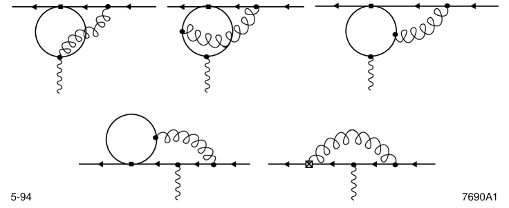
Figure 1: Feynman diagrams contributing to the mixing of the two-quark–two-squark operators (4.3) into the operator ${O_{\mathrm{LR}}^{3}}$. A full square denotes the insertion of a two-quark–two-squark operator, while an open square denotes a one-loop counterterm. Diagrams which are related to the ones above by reflection are not shown.

The actual two-loop calculation of the mixing of the two-quark–two-squark operators (4.3) into the magnetic moment operators is performed analogously to the corresponding calculation with insertions of four-quark operators (see e.g. [4]). In figure 1 we show the relevant diagrams and one-loop counterterms contributing to the mixing of the two-quark–two-squark operators into the operator ${O_{\mathrm{LR}}^{3}}$. As we prefer to work off-shell, we have to consider only 1-PI diagrams. The main advantage is a simplification of the extraction of the divergent parts of interest by focussing on the coefficients of the tensor structures that are defined by our basis (2).

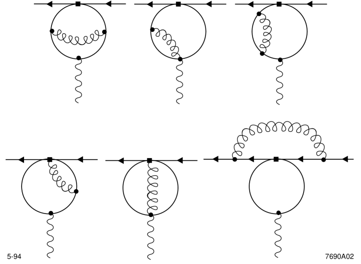
Figure 2: Feynman diagrams whose contribution to the mixing vanishes after application of the equations of motion.

Similarly to the corresponding calculations with insertions of four-fermion operators, using the equations of motion (3.1.4) greatly reduces the computational effort. Figure 2 shows typical diagrams which do not contribute because their sum can be shown to be proportional to $(\gamma_{\mu}q^{2}-q_{\mu}q\hskip-4.49997pt/)$, and therefore need not be calculated.

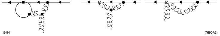
Figure 3: Additional Feynman diagrams which contribute to the mixing of the two-quark–two-squark operators into the operator ${O_{\mathrm{LR}}^{2}}$.

In the case of the mixing into ${O_{\mathrm{LR}}^{2}}$, due to the non-Abelian interactions of the gluons, we have to consider the additional diagrams and counterterms shown in figure 3.

We obtained the following mixing coefficients ($N=3$):

$$\hat{\gamma}=\bordermatrix{&{O_{\mathrm{LR}}^{2}}&{O_{\mathrm{LR}}^{3}}\cr\tilde{Q}_{\mathrm{LR}}^{1}&\frac{N^{2}-2}{8N}&\frac{Q_{\mathrm{t}}}{Q_{\mathrm{b}}}\frac{N^{2}-1}{4N}\cr\tilde{Q}_{\mathrm{LR}}^{2}&\frac{1}{4}&0\cr{\tilde{R}_{\mathrm{L}}^{1,a}}&\frac{N^{2}-2}{8N}&\frac{Q_{\mathrm{t}}}{Q_{\mathrm{b}}}\frac{N^{2}-1}{4N}\cr{\tilde{R}_{\mathrm{L}}^{2,a}}&-\frac{N^{2}-2}{16N}-\frac{N^{2}+2}{72N}&\left(-\frac{1}{4}\frac{Q_{\mathrm{t}}}{Q_{\mathrm{b}}}+\frac{1}{18}\right)\frac{N^{2}-1}{2N}\cr{\tilde{R}_{\mathrm{L}}^{3,a}}&-\frac{N^{2}-2}{16N}+\frac{N^{2}+2}{72N}&\left(-\frac{1}{4}\frac{Q_{\mathrm{t}}}{Q_{\mathrm{b}}}-\frac{1}{18}\right)\frac{N^{2}-1}{2N}\cr{\tilde{R}_{\mathrm{L}}^{4,a}}&\frac{1}{4}&0\cr{\tilde{R}_{\mathrm{L}}^{5,a}}&-\frac{1}{8}&0\cr{\tilde{R}_{\mathrm{L}}^{6,a}}&-\frac{1}{8}&0\cr}$$ (61)

In addition we need the mixing among the two-quark–two-squark operators, where the squarks are of the same kind,

$$\hat{\gamma}=\bordermatrix{&\tilde{Q}_{\mathrm{LR}}^{1}&\tilde{Q}_{\mathrm{LR}}^{2}&{\tilde{R}_{\mathrm{L}}^{1,a}}&{\tilde{R}_{\mathrm{L}}^{2,a}}&{\tilde{R}_{\mathrm{L}}^{3,a}}&{\tilde{R}_{\mathrm{L}}^{4,a}}&{\tilde{R}_{\mathrm{L}}^{5,a}}&{\tilde{R}_{\mathrm{L}}^{6,a}}\cr\tilde{Q}_{\mathrm{LR}}^{1}&\frac{1}{2}&-\frac{3}{2}&0&0&0&0&0&0\cr\tilde{Q}_{\mathrm{LR}}^{2}&0&-4&0&0&0&0&0&0\cr{\tilde{R}_{\mathrm{L}}^{1,a}}&\frac{9}{2}&-\frac{3}{2}&-4&0&0&0&0&0\cr{\tilde{R}_{\mathrm{L}}^{2,a}}&-\frac{1}{2}&\frac{3}{2}&0&-\frac{25}{6}&\frac{1}{6}&0&\frac{13}{18}&-\frac{13}{18}\cr{\tilde{R}_{\mathrm{L}}^{3,a}}&-4&0&0&\frac{1}{6}&-\frac{25}{6}&0&-\frac{13}{18}&\frac{13}{18}\cr{\tilde{R}_{\mathrm{L}}^{4,a}}&0&0&0&0&0&-4&0&0\cr{\tilde{R}_{\mathrm{L}}^{5,a}}&\frac{3}{2}&-\frac{1}{2}&0&0&0&0&-2&-2\cr{\tilde{R}_{\mathrm{L}}^{6,a}}&-\frac{3}{2}&\frac{1}{2}&0&0&0&0&-2&-2\cr}$$ (62)

and for different types of squarks ($a\neq b$):

$$\hat{\gamma}=\bordermatrix{&\tilde{R}_{\mathrm{L}}^{2,b}&\tilde{R}_{\mathrm{L}}^{3,b}&\tilde{R}_{\mathrm{L}}^{5,b}&\tilde{R}_{\mathrm{L}}^{6,b}\cr{\tilde{R}_{\mathrm{L}}^{2,a}}&\frac{1}{12}&-\frac{1}{12}&-\frac{1}{36}&\frac{1}{36}\cr{\tilde{R}_{\mathrm{L}}^{3,a}}&-\frac{1}{12}&\frac{1}{12}&\frac{1}{36}&-\frac{1}{36}\cr}$$ (63)

Note that there is a mixing of some of the two-quark–two-squark operators into four-fermion operators:

$$\hat{\gamma}=\bordermatrix{&S_{3}&S_{4}&S_{5}&S_{6}\cr{\tilde{R}_{\mathrm{L}}^{2,a}}&-\frac{1}{36}&\frac{1}{12}&-\frac{1}{36}&\frac{1}{12}\cr{\tilde{R}_{\mathrm{L}}^{3,a}}&\frac{1}{36}&-\frac{1}{12}&\frac{1}{36}&-\frac{1}{12}\cr}$$ (64)

If there are squarks lighter than the top quark, we also have to take into account the mixing of the four-fermion operators into the operators $\tilde{R}$:

$$\hat{\gamma}=\bordermatrix{&{\tilde{R}_{\mathrm{L}}^{2,a}}&{\tilde{R}_{\mathrm{L}}^{3,a}}&{\tilde{R}_{\mathrm{L}}^{5,a}}&{\tilde{R}_{\mathrm{L}}^{6,a}}\cr S_{1}&0&0&0&0\cr S_{2}&\frac{1}{3}&-\frac{1}{3}&-\frac{1}{9}&\frac{1}{9}\cr S_{3}&\frac{2}{3}&-\frac{2}{3}&-\frac{2}{9}&\frac{2}{9}\cr S_{4}&\frac{n_{f}}{3}&-\frac{n_{f}}{3}&-\frac{n_{f}}{9}&\frac{n_{f}}{9}\cr S_{5}&0&0&0&0\cr S_{6}&\frac{n_{f}}{3}&-\frac{n_{f}}{3}&-\frac{n_{f}}{9}&\frac{n_{f}}{9}\cr}$$ (65)

In principle there is also a QCD-induced mixing into operators with two quarks and two down-type squarks, which we also would have to include if we were considering the contributions induced by gluinos and neutralinos. In most scenarios, the mass splitting of down-type squarks is much smaller than for up-type squarks. For the supersymmetric contributions to be numerically relevant the lightest squark (which is usually the lightest stop) must be significantly lighter than the other squarks. As has been argued in the introduction, contributions from these operators are strongly suppressed, and also inclusion of these operators into the mixing would lead to only a minor effect compared to other neglected corrections. Furthermore, all Wilson coefficients that contribute to mixing via (63,64) are proportional to $\cot^{2}\beta$ and therefore suppressed in the large-$\tan\beta$ limit.

Again, if we cross the threshold $\mu=\tilde{m}_{a}$ of squark $\tilde{u}_{a}$, the matching contribution vanishes to leading order, and the operators $\tilde{O}^{a}$, $\tilde{R}^{a}$ are simply removed. We will also add in the corresponding subleading contributions each time a pair ($a,j$) of squarks and charginos has been integrated out, i.e. at $\mu=\min(\tilde{m}_{a},\tilde{m}_{j})$.

5 Results and Discussions

As the full anomalous dimension matrix is quite large and changes its structure every time we cross a threshold, it would be a big effort to diagonalize it in every step. It is much simpler to directly evaluate the solution (8) of the RGE numerically. Before we proceed, let us comment on some simplifications that result from the use of the equations of motion, since we are eventually only interested in the coefficient of the magnetic moment operators at the $b$ scale.

First we note that the operators $Q_{\mathrm{LR}}$ and ${R_{\mathrm{L}}^{1}}$, and in the case of $m_{\mathrm{H}^{\pm}}<m_{\mathrm{t}}$ their “primed” counterparts, which appear in intermediate stages of the calculations, turn out to be superfluous as they do not give any contribution in the process of matching, nor do they mix into any other operator. Second, although the coefficient of ${P_{\mathrm{L}}^{2}}$ does get matching contributions, and many operators mix into it, it can be ignored, since it vanishes after applying the equations of motion. Third, the operators ${R_{\mathrm{L}}^{2}}$ and ${R_{\mathrm{L}}^{3}}$ mix only into ${P_{\mathrm{L}}^{2}}$, which vanishes by equations of motion, and may therefore be omitted from the beginning. Extending this reasoning to ${R_{\mathrm{L}}^{2}}^{\prime}$, ${R_{\mathrm{L}}^{3}}^{\prime}$, $W_{\mathrm{LR}}^{1,j}$, $W_{\mathrm{L}}^{j}$ and ${\tilde{R}_{\mathrm{L}}^{4,a}}$ shows that they may also be disregarded.

Next, one may convince oneself that the apparent zeroth-order mixing of some operators (see eqs. (35), (60)) vanishes after application of the equations of motion, so all mixing occurs at order $(g_{3}^{2}/8\pi^{2})$, as promised.

Let us first rediscuss the effect of the QCD corrections to the Standard Model contribution. For the contribution from the W-$t$-loop there is a QCD enhancement of the coefficients $C_{{O_{\mathrm{LR}}^{2}}}^{\mathrm{eff}}(m_{\mathrm{W}})$ and $C_{{O_{\mathrm{LR}}^{3}}}^{\mathrm{eff}}(m_{\mathrm{W}})$ of the order of 10–18% and 15–22% for $m_{\mathrm{t}}=130\ldots 250\,\mathrm{GeV}$, respectively, which after scaling down to $\mu=m_{\mathrm{b}}$ and including the contribution from the four-fermion operators leads to an additional enhancement of the decay rate within the SM of the order of 12–23% [13], compared to the case when both $t$ and W are integrated out at $\mu=m_{\mathrm{W}}$. This large correction, which seems to compare quite well with the naive estimate given in the introduction, is a confirmation that a full next-to-leading order calculation is quite important.

The magnitude of this effect may be understood by solving the renormalization group equation for the leading terms. After application of the equations of motion, their contribution turns out to be quite simple:

$$\left.C_{O_{\mathrm{LR}}^{2}}^{\mathrm{eff}}(m_{\mathrm{W}})\right|_{\mathrm{SM}} = -\frac{5}{24}\left(\frac{\alpha_{3}(m_{\mathrm{t}})}{\alpha_{3}(m_{\mathrm{W}})}\right)^{14/23}+\frac{1}{3}+\mathrm{(subleading)}$$

$$\left.C_{O_{\mathrm{LR}}^{3}}^{\mathrm{eff}}(m_{\mathrm{W}})\right|_{\mathrm{SM}} = \frac{5}{3}\left(\frac{\alpha_{3}(m_{\mathrm{t}})}{\alpha_{3}(m_{\mathrm{W}})}\right)^{14/23}-\frac{8}{3}+\mathrm{(subleading)}$$ (66)

The reason that (5) leads to positive corrections is essentially due to the fact that the effective matching contributions at $\mu=m_{\mathrm{t}}$ (3.1.1) and at $\mu=m_{\mathrm{W}}$ (3.1.3) have opposite sign (which is a remnant of the GIM mechanism), and therefore lead to coefficients of opposite sign but comparable magnitude of the first two terms on the right-hand sides of (5). It has long been known [34] that the QCD corrections tend to soften the GIM-cancellations between different up-type quarks if they are nearly degenerate; but even for a heavy top quark (i.e. $m_{\mathrm{t}}\gg m_{\mathrm{W}}$) there remains a finite enhancement, as can be explicitly seen from these expressions. Note that (5) gives only the leading terms; the subleading terms being suppressed by only a factor of $(m_{\mathrm{W}}/m_{\mathrm{t}})^{2}$.

Next let us turn to the contribution from the loop with a charged Higgs. For this case we have solved the renormalization group equation numerically, using as input parameters:

$$m_{\mathrm{b}}=4.5\,\mathrm{GeV},\quad m_{\mathrm{t}}=175\,\mathrm{GeV},$$

$$m_{\mathrm{W}}=80.22\,\mathrm{GeV},\quad\alpha_{3}(m_{\mathrm{Z}})=0.123$$

Figure 4: Correction (67) to the coefficients of ${O_{\mathrm{LR}}^{3}}(m_{\mathrm{b}})$ from a loop with $t$ quark and charged Higgs with leading QCD corrections from large mass splitting to the case when both particles are integrated out at $\mu=m_{\mathrm{W}}$. The mass of the $t$ quark is assumed to be 175 GeV. The dotted, long-dashed, dashed and solid line correspond to $\tan\beta=1.5,\,2,\,3,$ and 10, respectively.

The resulting correction

$$\delta_{\mathrm{H}^{\pm}}=\left.\frac{C_{O_{\mathrm{LR}}^{3}}^{\mathrm{eff}}(m_{\mathrm{b}})}{C_{O_{\mathrm{LR}}^{3}}^{\mathrm{eff,naive}}(m_{\mathrm{b}})}\right|_{{\mathrm{H}^{\pm}}}-1$$ (67)

to the “naive” result, obtained by integrating out $t$ and ${\mathrm{H}^{\pm}}$ simultaneously at the W scale, is shown in figure 4 for $m_{\mathrm{W}}<m_{\mathrm{H}^{\pm}}<750\,\mathrm{GeV}$ and $\tan\beta=1.5,\,2,\,3,$ and 10. At sufficiently large $\tan\beta$ (i.e. $\tan\beta>3$), the correction turns out to be essentially independent of $\tan\beta$. This is quite understandable since the $\tan\beta$-dependent pieces are actually proportional to $\cot^{2}\beta$.

For a light charged Higgs, i.e. $m_{\mathrm{H}^{\pm}}<m_{\mathrm{t}}$, there appears to be a further reduction of this contribution compared to the naive result. Indeed, in the limit of large $\tan\beta$, and assuming there is no light squark or gluino with mass below $m_{\mathrm{t}}$, one finds the following simple analytical result for the charged Higgs contribution, valid for $m_{\mathrm{b}}<\mu<m_{\mathrm{t}}$:

$$\left.C_{O_{\mathrm{LR}}^{2}}^{\mathrm{eff}}(\mu)\right|_{\mathrm{H}^{\pm}} = \frac{1}{4}\left(\frac{\alpha_{3}(m_{\mathrm{t}})}{\alpha_{3}(\mu)}\right)^{14/23}+\mathrm{(subl.)}+O(\cot^{2}\beta)$$ (68)

$$\left.C_{O_{\mathrm{LR}}^{3}}^{\mathrm{eff}}(\mu)\right|_{\mathrm{H}^{\pm}} = \frac{3}{4}\left(\frac{\alpha_{3}(m_{\mathrm{t}})}{\alpha_{3}(\mu)}\right)^{16/23}-2\left(\frac{\alpha_{3}(m_{\mathrm{t}})}{\alpha_{3}(\mu)}\right)^{14/23}+\mathrm{(subl.)}+O(\cot^{2}\beta)$$

Hence no enhancement occurs as in the case of the SM contribution; on the contrary, the leading coefficients get suppressed as they are run down from the $m_{\mathrm{t}}$, compared to the subleading terms which (according to our discussion in section 3.1.3) get only suppressed by the evolution from $\mu=m_{\mathrm{H}^{\pm}}$ down to $\mu=m_{\mathrm{b}}$. For sufficiently small $m_{\mathrm{H}^{\pm}}$, the additional QCD corrections are then essentially due to the running from $\mu=m_{\mathrm{t}}$ to $\mu=m_{\mathrm{H}^{\pm}}$. Note that our “corrections” are counted relative to the case when both particles in the loop are integrated out at the common scale $\mu=m_{\mathrm{W}}$, which is obtained from (68) by substituting $\alpha_{3}(m_{\mathrm{t}})\to\alpha_{3}(m_{\mathrm{W}})$. Thus, for $m_{\mathrm{H}^{\pm}}<m_{\mathrm{t}}$, integrating out $t$ and ${\mathrm{H}^{\pm}}$ at the $t$ scale appears to give a more accurate result than at $\mu=m_{\mathrm{H}^{\pm}}$ or $\mu=m_{\mathrm{W}}$.

On the other hand, for $m_{\mathrm{H}^{\pm}}>m_{\mathrm{t}}$ we found only a minor suppression of a few percent, which is essentially the result of a partial cancellation of the enhancement coming from the scaling between $m_{\mathrm{H}^{\pm}}$ and $m_{\mathrm{t}}$ (due to one negative eigenvalue of the submatrix (39) for the mixing of four-fermion operators), and of a reduction from the scaling between $m_{\mathrm{t}}$ to $m_{\mathrm{W}}$. Unfortunately, we were unable to obtain a simple analytical solution for this case.

In the case of the chargino contribution, things are more complicated, since one has to consider in general the dependence of the amplitude as a function of several parameters, namely the mass spectrum and the mixing angles for the charginos and the up-type squarks. However, it turns out that the essential features may already be studied for the case of sufficiently large $\tan\beta$, which is in the center of recent interest [11, 18, 20, 23, 24, 25]. In this case, the parameter $\lambda_{\mathrm{b}}$ (47) may become of the same order of magnitude as the parameter $\lambda_{\mathrm{t}}$. Assuming furthermore that the mixing in the squark sector is essentially the same as in the quark sector, which is quite natural in supergravity models where the soft SUSY-breaking is characterized by a common scalar mass at some unification scale, the quantities ${\cal G}$ and ${\cal H}$, as defined in (51), are then necessarily of the same order of magnitude, the terms proportional to the ratio $\tilde{m}_{j}/m_{\mathrm{b}}$ will dominate the amplitude, and the corrections become $\tan\beta$-independent.

In this particular limit, one can find an analytical result for the leading terms. For the case of the chargino being much lighter than the squark, the coefficients read:

$$\left.C_{O_{\mathrm{LR}}^{2}}^{\mathrm{eff}}(\mu)\right|_{\chi} = \tilde{C}\cdot\frac{1}{2}e^{14t/3}+\mathrm{(subl.)}+O(\cot^{2}\beta)$$

$$\left.C_{O_{\mathrm{LR}}^{3}}^{\mathrm{eff}}(\mu)\right|_{\chi} = \tilde{C}\cdot\left[-4e^{14t/3}+e^{16t/3}\left(\frac{15}{2}+\frac{4\pi}{2bQ_{\mathrm{b}}}\left(\frac{1}{\alpha_{3}(\mu)}-\frac{1}{\alpha_{3}(\tilde{m}_{a})}\right)\right)\right]+$$ (69)

$$+\mathrm{(subl.)}+O(\cot^{2}\beta)$$

where

$$\tilde{C} = {\cal G}^{*{ja\mathrm{s}}}{\cal H}^{{ja\mathrm{b}}}\cdot\frac{\tilde{m}_{j}}{m_{\mathrm{b}}}\left(\frac{m_{\mathrm{W}}}{\tilde{m}_{a}}\right)^{2}\;,\qquad t=\frac{1}{2b}\ln\left(\frac{\alpha_{3}(\mu)}{\alpha_{3}(\tilde{m}_{a})}\right)$$

while for the other case of a squark much lighter than a chargino, we get:

$$\left.C_{O_{\mathrm{LR}}^{2}}^{\mathrm{eff}}(\mu)\right|_{\tilde{q}} = \tilde{C}\cdot\left[\frac{99}{260}e^{14t/3}+\frac{1}{10}e^{t/2}+\frac{1}{52}e^{-4t}\right]+\mathrm{(subl.)}+O(\cot^{2}\beta)$$

$$\left.C_{O_{\mathrm{LR}}^{3}}^{\mathrm{eff}}(\mu)\right|_{\tilde{q}} = \tilde{C}\cdot\left[-\frac{198}{65}e^{14t/3}+\frac{495}{406}e^{16t/3}-\frac{96}{145}e^{t/2}-\frac{1}{91}e^{-4t}\right]+$$ (70)

$$+\mathrm{(subl.)}+O(\cot^{2}\beta)$$

where now

$$\tilde{C} = {\cal G}^{*{ja\mathrm{s}}}{\cal H}^{{ja\mathrm{b}}}\cdot\frac{m_{\mathrm{W}}^{2}}{\tilde{m}_{j}m_{\mathrm{b}}}\;,\qquad t=\frac{1}{2b}\ln\left(\frac{\alpha_{3}(\mu)}{\alpha_{3}(\tilde{m}_{j})}\right)$$

At first sight the terms proportional to $1/\alpha_{3}$ in (5) might be embarrassing, but a closer look shows that their difference is (to leading order) just some number times $\ln(\mu/\tilde{m}_{a})$ and therefore finite in the limit $\alpha_{3}\to 0$.

Unfortunately, the interpretation of these expressions is aggravated in both limiting cases since the number of free parameters in the general model is quite large, and due to eqs. (53) one has a supersymmetric version of the GIM mechanism, which leads to a partial cancellation of the leading terms under consideration. This renders it difficult to estimate the actual corrections due to the mass splitting between charginos and squarks by using (5) or (5).

Some features of these expressions may still be studied under the following assumptions: i) the squarks of the first two generations are degenerate with mass $\tilde{m}_{u}$, ii) the mixing in the squark sector is the same as in the quark sector (i.e. the gluino-quark-squark couplings are flavor-diagonal even in the mass eigenstate basis), and iii) the mass matrix for the stop is given (in the ($t_{\mathrm{L}},t_{\mathrm{R}}$) basis) by

$$M_{\tilde{t}}^{2} = \pmatrix{\tilde{m}^{2}_{t_{\mathrm{L}}}&\tilde{m}^{2}_{t_{\mathrm{LR}}}\cr\tilde{m}^{2}_{t_{\mathrm{LR}}}&\tilde{m}^{2}_{t_{\mathrm{R}}}\cr}$$ (71)

This mass matrix is diagonalized by a unitary matrix $T$,

$$TM_{\tilde{t}}^{2}T^{-1}=\pmatrix{\tilde{m}_{t_{1}}^{2}&0\cr 0&\tilde{m}_{t_{2}}^{2}\cr}$$ (72)

In this scenario, the quantities (51) take a particularly simple form:

$${\cal G}^{jal} \simeq V_{j1}T_{a1}-\lambda_{\mathrm{t}}V_{j2}T_{a2}\qquad\mathrm{for}\;l=b,s;\;a=\tilde{t}_{1,2}$$

$${\cal H}^{ja\mathrm{b}} \simeq \lambda_{\mathrm{b}}U_{j2}T_{a1}$$ (73)

while the sum over the squarks of the first two generations is determined by (53).

Let us for the moment neglect the mixing between $\tilde{t}_{\mathrm{L}}$ and $\tilde{t}_{\mathrm{R}}$, i.e. consider the case $\tilde{m}^{2}_{t_{\mathrm{LR}}}=0$, $T={\bf 1}$. Evaluating the first line of (5) to lowest order, we find for the contribution of a light chargino and after summing over the different squarks:

$$C_{O_{\mathrm{LR}}^{2}}^{\mathrm{eff}}(\tilde{m}_{j}) = \frac{1}{2}\lambda_{\mathrm{b}}U_{j2}V_{j1}\frac{\tilde{m}_{j}}{m_{\mathrm{b}}}\frac{m_{\mathrm{W}}^{2}}{\tilde{m}^{2}_{u}}\left(\frac{\tilde{m}^{2}_{j}}{\tilde{m}^{2}_{u}}\right)^{\frac{14}{3}\hat{\alpha}_{3}}\left[\left(\frac{\tilde{m}^{2}_{u}}{\tilde{m}^{2}_{t_{\mathrm{L}}}}\right)^{1+\frac{14}{3}\hat{\alpha}_{3}}-1\right]+$$ (74)

$$+O(\hat{\alpha}_{3}^{2})+\mathrm{(subl.)}+O(\cot^{2}\beta)$$

with the abbreviation

$$\hat{\alpha}_{3} = \frac{\alpha_{3}(\tilde{m}_{j})}{4\pi}$$

Similar, although rather lengthy expressions are obtained if the mixing between $\tilde{t}_{\mathrm{L}}$ and $\tilde{t}_{\mathrm{R}}$ is taken into account, and analogous results are found for the other coefficients in (5) and (5). As has already been pointed out in [23], the sign of the product $U_{j2}V_{j1}$ depends on the sign of $\mu_{\mathrm{h}}$, so that this leading contribution for large $\tan\beta$ can have either sign.

A closer look at (74) shows two counteracting effects: a reduction of the leading coefficient due to QCD running from $\tilde{m}_{u}$ down to $\tilde{m}_{j}$, while the term in square brackets shows an enhancement due to a “QCD-softening” of the GIM cancellation, independent on whether $\tilde{m}_{t_{\mathrm{L}}}$ is larger or smaller than $\tilde{m}_{u}$. The actual size of the corrections depends of course on the mass splitting between the squarks as well as on the splitting between the mass of the chargino and the squarks; since squarks can be an order or magnitude heavier than the lightest chargino, we estimate this coefficient to be of the order of

$$\frac{14}{3}\frac{\alpha_{3}(\tilde{m}_{j})}{4\pi}\times\left(\ln\frac{\tilde{m}_{u}}{\tilde{m}_{j}},\;\ln\frac{\tilde{m}_{u}}{\tilde{m}_{t}}\right)\vbox to4.30554pt{\vss\hbox{ $\stackrel{{\scriptstyle{\scriptstyle<}}}{{{\scriptstyle\sim}}}$ }\vss}15\%$$

Similar results are found when analyzing the other expressions, so we will in general expect corrections up to $O(15\%)$ with either sign. An exceptional situation occurs when, due to these super-GIM cancellations, the lowest-order contribution to ${O_{\mathrm{LR}}^{3}}$ is accidentally lower than to ${O_{\mathrm{LR}}^{2}}$ by orders of magnitude, since the above reasoning did not take into account the mixing of ${O_{\mathrm{LR}}^{2}}$ into ${O_{\mathrm{LR}}^{3}}$ for scales below the heavy thresholds. In this case a sensible answer is obtained only when using the full expressions.

6 Conclusions

We have extended the calculation of the leading QCD corrections for the inclusive $b\to s\gamma$ decay to the MSSM in the framework of effective field theories. It was shown that it is important to properly treat the high-energy scale at which the particles in the loop are integrated out, as well as how to calculate the QCD corrections between if the masses of the particles in the loop are vastly different. To this end, we have calculated the leading order anomalous dimension matrices for the operators for the various scenarios that are relevant to this process in the MSSM.

We found that, while the SM contribution to the Wilson coefficients at the weak scale gets enhanced in the limit of a heavy top quark by about 15–20%, the contribution from a loop with a charged Higgs gets actually slightly reduced by a few percent. For the contribution from the chargino loops the result depends strongly on the mass spectrum of the squarks and the charginos as well as on the mixing angles. Typically, one expects corrections up to the order of 15% with either sign, which is however less than the enhancement of the SM contribution.

Given a range of values for the inclusive decay, if one applies the above results to a parameter space analysis for a particular SUSY model, one will essentially find a relaxation of the bounds on the mass of the charged Higgs, especially in the region of large $\tan\beta$. The impact of the modification of the QCD corrections for the chargino loop contribution is not seen so easily, but we expect a smooth deformation of contours in analyses like [11, 25], with the strongest effect in those regions where the lowest order contribution to the coefficient $C_{O_{\mathrm{LR}}^{3}}$ is small although the chargino is relatively light.

Finally we would like to point out that for the inclusive decay rate, even after taking into account the real gluon emission and virtual corrections below the $b$ scale [35], the leading order prediction remains uncertain by about 25% due to the residual scale dependence alone [10, 12] (for the amplitude it is of the order 10–15%). Once a full next-to-leading order calculation is available for the SM, it may be combined with the above results to obtain predictions in the MSSM with comparable precision.

Appendix A Wilson coefficients at one loop

We quote here the results for the Wilson coefficients at one-loop order when both particles in the loop are integrated out at a common scale. These results will be used for the determination of subleading terms. They also provide an important cross-check for the leading terms obtained by the calculation in the effective theory, as well as for some of the entries in the anomalous dimension matrix.

We find it convenient to use the following functions that appear in the evaluation of the coefficients of the basis operators:

$$F_{1}(x) = \frac{x^{2}-5x-2}{12(x-1)^{3}}+\frac{x\ln x}{2(x-1)^{4}}$$

$$F_{2}(x) = \frac{2x^{2}+5x-1}{12(x-1)^{3}}-\frac{x^{2}\ln x}{2(x-1)^{4}}$$

$$F_{3}(x) = \frac{x-3}{2(x-1)^{2}}+\frac{\ln x}{(x-1)^{3}}$$

$$F_{4}(x) = \frac{x+1}{2(x-1)^{2}}-\frac{x\ln x}{(x-1)^{3}}$$ (75)

These functions are identical with those given in the appendix of ref. [17]. Some of their properties are:

$$F_{1}\left(\frac{1}{x}\right)=xF_{2}(x),\quad F_{2}\left(\frac{1}{x}\right)=xF_{1}(x),\quad F_{4}\left(\frac{1}{x}\right)=xF_{4}(x)$$

$$F_{1}(x)+F_{2}(x)=\frac{1}{2}F_{4}(x)=\frac{1}{4}-\frac{1}{2}xF_{3}(x)$$

$$xF_{1}(x)+F_{2}(x)=\frac{1}{12}$$

$$F_{3}\left(\frac{1}{x}\right)=-x\left(F_{3}(x)+2F_{4}(x)\right)+\frac{x\ln x}{x-1}$$ (76)

A.1 Standard Model loop contributions

Integrating out the W, the charged would-be Goldstone bosons and an up-type quark simultaneously, we obtain the one-loop expression of the Wilson coefficients of the effective Hamiltonian (1):

$$C_{{O_{\mathrm{LR}}^{1}}} = -xF_{4}(x)$$

$$C_{{O_{\mathrm{LR}}^{2}}} = \frac{Q_{\mathrm{b}}}{Q_{\mathrm{t}}}C_{{O_{\mathrm{LR}}^{3}}}=-\frac{x}{2}\left(F_{3}(x)+F_{4}(x)\right)$$

$$C_{{P^{1,1}_{\mathrm{L}}}} = C_{{P^{1,3}_{\mathrm{L}}}}=\frac{1}{3}(x+2)\left(2F_{2}(x)+F_{3}(x)+2F_{4}(x)\right)$$

$$C_{{P^{1,2}_{\mathrm{L}}}} = \frac{2}{3}(x+2)\left(F_{2}(x)-F_{3}(x)-2F_{4}(x)\right)$$

$$C_{{P^{1,4}_{\mathrm{L}}}} = (x-2)F_{4}(x)$$ (77)

$$C_{{P_{\mathrm{L}}^{2}}} = \frac{1}{Q_{\mathrm{b}}}(x+2)\left(\frac{1}{2}F_{3}(x)+F_{4}(x)-\frac{\ln(x)}{6(x-1)}\right)$$

$$C_{{P_{\mathrm{L}}^{4}}} = \frac{1}{Q_{\mathrm{b}}}\left(3-2xF_{3}(x)-5xF_{4}(x)\right)$$

Here $x=(m_{q}/m_{\mathrm{W}})^{2}$. Note that for large $x$ all coefficient functions are bounded, except for $C_{P_{\mathrm{L}}^{2}}$, which grows logarithmically with $x$. For small $x$, $C_{P^{1,1}_{\mathrm{L}}}$, $C_{P^{1,2}_{\mathrm{L}}}$, $C_{P^{1,3}_{\mathrm{L}}}$ and $C_{P_{\mathrm{L}}^{2}}$ diverge logarithmically.

A.2 Charged Higgs loop contributions

Integrating out the charged Higgs and an up-type quark simultaneously, the corresponding expressions are ($y=(m_{q}/m_{\mathrm{H}^{\pm}})^{2}$):

$$C_{{O_{\mathrm{LR}}^{1}}} = yF_{4}(y)$$

$$C_{{O_{\mathrm{LR}}^{2}}} = \frac{Q_{\mathrm{b}}}{Q_{\mathrm{t}}}C_{{O_{\mathrm{LR}}^{3}}}=\frac{y}{2}\left(F_{3}(y)+F_{4}(y)\right)$$

$$C_{{P^{1,1}_{\mathrm{L}}}} = C_{{P^{1,3}_{\mathrm{L}}}}=\frac{1}{3}y\left(2F_{2}(y)+F_{3}(y)+2F_{4}(y)\right)\cot^{2}\beta$$

$$C_{{P^{1,2}_{\mathrm{L}}}} = \frac{2}{3}y\left(F_{2}(y)-F_{3}(y)-2F_{4}(y)\right)\cot^{2}\beta$$

$$C_{{P^{1,4}_{\mathrm{L}}}} = -Q_{\mathrm{b}}C_{{P_{\mathrm{L}}^{4}}}=yF_{4}(y)\cot^{2}\beta$$ (78)

$$C_{{P_{\mathrm{L}}^{2}}} = \frac{1}{Q_{\mathrm{b}}}y\left(\frac{1}{2}F_{3}(y)+F_{4}(y)-\frac{\ln(y)}{6(y-1)}\right)\cot^{2}\beta$$

A.3 Chargino loop contributions

Finally we give the expressions for integrating out a chargino and an up-type squark. Setting $z=(\tilde{m}_{j}/\tilde{m}_{a})^{2}$, where $m_{j}$ and $m_{a}$ represent the mass of the chargino $\chi_{j}$ and of the up-type squark $\tilde{u}_{a}$ respectively, and using the couplings defined in eq. (51), one finds

$$C_{{O_{\mathrm{LR}}^{1}}} = {\cal G}^{*{ja\mathrm{s}}}{\cal H}^{{ja\mathrm{b}}}\cdot\frac{\tilde{m}_{j}}{m_{\mathrm{b}}}\left(\frac{m_{\mathrm{W}}}{\tilde{m}_{a}}\right)^{2}\cdot(-2)F_{4}(z)$$

$$C_{{O_{\mathrm{LR}}^{2}}} = 0$$

$$C_{{O_{\mathrm{LR}}^{3}}} = {\cal G}^{*{ja\mathrm{s}}}{\cal H}^{{ja\mathrm{b}}}\cdot\frac{\tilde{m}_{j}}{m_{\mathrm{b}}}\left(\frac{m_{\mathrm{W}}}{\tilde{m}_{a}}\right)^{2}\cdot\frac{1}{Q_{\mathrm{b}}}\left(F_{3}(z)+F_{4}(z)\right)$$

$$C_{{P^{1,1}_{\mathrm{L}}}} = C_{{P^{1,3}_{\mathrm{L}}}}={\cal G}^{*{ja\mathrm{s}}}{\cal G}^{{ja\mathrm{b}}}\cdot\left(\frac{m_{\mathrm{W}}}{\tilde{m}_{a}}\right)^{2}\cdot\frac{1}{3}\left[4F_{2}(z)+\frac{1}{z}F_{3}\left(\frac{1}{z}\right)\right]$$

$$C_{{P^{1,2}_{\mathrm{L}}}} = {\cal G}^{*{ja\mathrm{s}}}{\cal G}^{{ja\mathrm{b}}}\cdot\left(\frac{m_{\mathrm{W}}}{\tilde{m}_{a}}\right)^{2}\cdot\frac{2}{3}\left[2F_{2}(z)-\frac{1}{z}F_{3}\left(\frac{1}{z}\right)\right]$$

$$C_{{P^{1,4}_{\mathrm{L}}}} = 0$$ (79)

$$C_{{P_{\mathrm{L}}^{2}}} = {\cal G}^{*{ja\mathrm{s}}}{\cal G}^{{ja\mathrm{b}}}\cdot\left(\frac{m_{\mathrm{W}}}{\tilde{m}_{a}}\right)^{2}\cdot\left(-\frac{2}{Q_{\mathrm{b}}}\right)\left(\frac{1}{2}F_{3}(z)+F_{4}(z)-\frac{\ln(z)}{6(z-1)}\right)$$

$$C_{{P_{\mathrm{L}}^{4}}} = {\cal G}^{*{ja\mathrm{s}}}{\cal G}^{{ja\mathrm{b}}}\cdot\left(\frac{m_{\mathrm{W}}}{\tilde{m}_{a}}\right)^{2}\cdot\left(\frac{2}{Q_{\mathrm{b}}}\right)F_{4}(z)$$

After application of the equations of motion, these expressions are consistent with the corresponding expressions in [17].

References

- [1] R. Ammar et al. (CLEO Collaboration), Phys. Rev. Lett. 71 (1993) 674
- [2] T. Inami, C.S. Lim, Prog. Theor. Phys. 65 (1981) 297
- [3] R. Grigjanis, P.J. O’Donnell, M. Sutherland, H. Navelet, Phys. Rep. 228 (1993) 93
- [4] B. Grinstein, R. Springer, M. Wise, Phys. Lett. B202 (1988) 138; Nucl. Phys. B339 (1990) 269
- [5] R. Grigjanis, P.J. O’Donnell, M. Sutherland, H. Navelet, Phys. Lett. B213 (1988) 355; ibid. B286 (1992) 413(E)
- [6] G. Cella, G. Curci, G. Ricciardi, A. Viceré, Phys. Lett. B248 (1990) 181; Phys. Lett. B325 (1994) 227; preprint IFUP-TH 9/94, HUTP-94/A001, hep-ph/9406203, June 1994
- [7] M. Misiak, Phys. Lett. B269 (1991) 161; Nucl. Phys. B393 (1993) 23; Phys. Lett. B321 (1994) 113
- [8] K. Adel, Y.P. Yao, Mod. Phys. Lett. A8 (1993) 1679; preprint UM-TH-93-20, IP-ASTP-29-93, hep-ph/9308349
- [9] M. Ciuchini, E. Franco, G. Martinelli, L. Reina, L. Silvestrini, Phys. Lett. B316 (1993) 127; M. Ciuchini, E. Franco, L. Reina, L. Silvestrini, preprint ROME-973-1993, hep-ph/9311357
- [10] A. Ali, C. Greub, Z. Phys. C60 (1993) 433
- [11] F. Borzumati, preprint DESY 93-090, hep-ph 9310212, August 1993
- [12] A. Buras, M. Misiak, M. Münz, S. Pokorski, MPI-Ph/93-73, TUM-T31-50/93, hep-ph 9311345
- [13] P. Cho, B. Grinstein, Nucl. Phys. B365 (1991) 279; Erratum: ibid., (in print)
- [14] H. Haber, G. Kane, Phys. Rep. 117 (1985) 75
- [15] S. Bertolini, F. Borzumati, A. Masiero, Phys. Lett. B192 (1987) 437; Nucl. Phys. B294 (1987) 321
- [16] H.P. Nilles, Phys. Rep. 110 (1984) 1; A.B. Lahanas, D.V. Nanopoulos, Phys. Rep. 145 (1987) 1. For a recent introduction to supergravity phenomenology see e.g. R. Arnowitt, P. Nath, Lecture at Swieca Summer School, Campos do Jordao, Brasil, 1993, preprint CTP-TAMU-52/93
- [17] S. Bertolini, F. Borzumati, A. Masiero, G. Ridolfi, Nucl. Phys. B353 (1991) 591
- [18] N. Oshimo, Nucl. Phys. B404 (1993) 20
- [19] J.L. Lopez, D. Nanopoulos, G.T. Park, Phys. Rev. D48 (1993) 974
- [20] M.A. Diaz, Phys. Lett. B304 (1993) 278; Phys. Lett. B322 (1994) 207
- [21] R. Barbieri, G.F. Giudice, Phys. Lett. B309 (1993) 86
- [22] Y. Okada, Phys. Lett. B315 (1993) 119
- [23] R. Garisto, J.N. Ng, Phys. Lett. B315 (1993) 372
- [24] J.S. Hagelin, S. Kelley, T. Tanaka, Nucl. Phys. B415 (1994) 293
- [25] S. Bertolini, F. Vissani, preprint SISSA 40/94/EP, hep-ph/9403397
- [26] G. Bhattacharyya, A. Raychaudhuri, preprint CERN-TH.7245/94, hep-ph/9405235, May 1994
- [27] E. Witten, Nucl. Phys. B122 (1977) 109
- [28] S. Weinberg, Phys. Lett. B91 (1979) 51
- [29] A. Cohen, H. Georgi, B. Grinstein, Nucl. Phys. B232 (1984) 61
- [30] H. Georgi, Nucl. Phys. B363 (1991) 301
- [31] H. Georgi, Ann. Rev. Nucl. Part. Sci. 43 (1993) 209
- [32] T. Appelquist, J. Carazzone, Phys. Rev. D11 (1975) 2856
- [33] L. Abbott, Nucl. Phys. B185 (1981) 189
- [34] F. Gilman, M. Wise, Phys. Rev. D21 (1980) 3150
- [35] A. Ali, C. Greub, Phys. Lett. B259 (1991) 182; Z. Phys. C49 (1991) 431