SOFT PION EMISSION IN
SEMILEPTONIC $B$-MESON DECAYS

Abstract

An analysis of semileptonic decays of $B$ mesons with the emission of a single soft pion is presented in the framework of the heavy-quark limit using an effective Lagrangian which implements chiral and heavy-quark symmetries. The analysis is performed at leading order of the chiral and inverse heavy mass expansions. In addition to the ground state heavy mesons some of their resonances are included. The estimates of the various effective coupling constants and form factors needed in the analysis are obtained using a chiral quark model. As the main result, a clear indication is found that the $0^{+}$ and $1^{+}$ resonances substantially affect the decay mode with a $D^{\ast}$ in the final state, and a less dramatic effect is also noticed in the $D$ mode. An analysis of the decay spectrum in the $D^{(\ast)}-\pi$ squared invariant mass is carried out, showing the main effects of including the resonances. The obtained rates show promising prospects for studies of soft pion emission in semileptonic $B$-meson decays in a $B$-meson factory where, modulo experimental cuts, about $10^{5}$ such decays in the $D$ meson mode and $10^{4}$ in the $D^{\ast}$ mode could be observed per year.

I Introduction

Semileptonic $B\rightarrow D^{(\ast)}$ decays with emission of a single pion may soon be established at CLEO or ARGUS, as well as at the planned $B$-meson factory. These decays, denoted $B_{\ell 4}$ in the rest of this article, complete the list of this category of decays which includes $K_{\ell 4}$ and $D_{\ell 4}$. There are fundamental differences among these three decays, which make their study very interesting. In particular, $K_{\ell 4}$ decays can be studied within chiral perturbation theory ($\chi$PT) over the whole final-state phase space as the resulting pions are soft [1]. $D_{\ell 4}$ decays [2] are much harder to study because, with the exception of a small fraction of phase space, the final state involves light mesons with relatively large energies. This makes the use of an effective theory not viable.

$B_{\ell 4}$ decays offer new theoretical possibilities. As a whole, they are difficult to predict because the kinematic domain of the daughter pion ranges from the soft limit, to be properly defined later, to a high energy limit. However, it is possible to restrict the study to the soft-pion limit, where one can make use of the powerful constraints resulting from heavy quark spin-flavor symmetry and chiral symmetry.

In this work we study the soft-pion domain in $B_{\ell 4}$ decays, for which the effective chiral Lagrangian approach combined with the inverse heavy mass expansion [3] provides a consistent theoretical framework. In a strict sense, it turns out that the soft-pion domain represents about 80% of the $B_{\ell 4}$ rate in the $D$ mode and about 10% in the $D^{\ast}$ mode. Here the large fraction in the D-mode is mostly due to the inclusion of the cascade decay $B\rightarrow\ell\bar{\nu}D^{\ast}\rightarrow\ell\bar{\nu}D\pi$. Since, according to a rough estimate, the total branching ratio for the $B_{\ell 4}$ decay is about 1% (0.2 %) in the $D$ ($D^{\ast}$) mode, it seems that experimental access to the soft-pion domain in the foreseable future, such as at a $B$ meson factory, is clearly possible.

Perhaps the most compelling motivation for studying $B_{\ell 4}$ decays is the overall current status of the semileptonic decays of $B$ mesons. The measured inclusive semileptonic branching ratio is $11.1\pm 0.3$ %, while the sum of measured exclusive semileptonic branching fractions is significantly less than this. In particular, the elastic modes $B\to De\nu$ and $B\to D^{*}e\nu$ account for only about 60 % of the total semileptonic branching fraction [4] ($b\to u$ modes are expected to be suppressed by $|V_{bu}|^{2}/|V_{bc}|^{2}\approx 0.01$). Understanding the so-called inelastic modes, such as those we discuss here, is therefore crucial to resolving the apparent discrepancies among the measurements.

Another interesting aspect of $B_{\ell 4}$-decays is that they may give an indication of resonance effects (especially $D$ meson resonances). At present, the only well established resonances are the two $P$-wave objects $D_{1}$ and $D_{2}$, with $J^{P}=1^{+},\,2^{+}$, respectively. States that may contribute significantly to $B_{\ell 4}$ decays, and hence which may be observed in such decays, include the remaining lowest-lying $P$-wave states (with $J^{P}=0^{+},\,1^{+}$), two of the lowest lying $D$-wave states ($J^{P}=1^{-},\,2^{-}$), and the first radially excited $S$-wave states ($J^{P}=0^{-},\,1^{-}$). It turns out that the well established $D_{1}$ and $D_{2}$ states [5] do not play a role in the present analysis, while only the $S$-wave radially excited $D$ mesons offer any opportunity for direct discovery using the $B_{\ell 4}$ decays, as they are the only ones with a small enough width to show up as a resonance feature in the decay spectrum.

From the theoretical standpoint, the soft-pion limit is particularly interesting, as chiral symmetry and spin-flavor symmetry determine to a large extent the different decay amplitudes, in terms of a few low-energy constants and universal form factors. These form factors are associated with the matrix elements of the charged $b\rightarrow c$ electroweak current between the relevant heavy meson states, and the low-energy constants determine the amplitudes of the strong interaction transitions mediated by the soft pion.

Another area of interest in $B_{\ell 4}$ decays is their contribution to $\rho$, the slope of the Isgur-Wise function which, in turn, impacts on the extraction of $|V_{cb}|$ from data. Bjorken, Dunietz and Taron [6] have obtained a sum rule that relates the slope of the Isgur-Wise function for the elastic decays $B\to D\ell\nu$ to the form factors that describe the inelastic semileptonic decays. The decays that we consider here provide the leading resonant and non-resonant contribution to this quantity.

These decays have been analyzed in the framework we explore by a number of authors. $B\to D\pi e\nu$ has been treated by Lee, Lu and Wise [7], and by Cheng et al. [8], while Lee [9] and Cheng et al. [8] have examined $B\to D^{*}\pi e\nu$. In these analyses, only the ground state mesons, the $D$, $D^{*}$, $B$ and $B^{*}$ were included, which amounts to keeping only those contributions wich are leading at the zero recoil point $v\cdot v^{\prime}=1$, $v$ and $v^{\prime}$ being the four velocities of the $B$ and $D$ mesons, respectively. In addition, we note that only Cheng et al. went on to estimate branching fractions and evaluate the differential decay spectra.

In this work we include resonances which contribute at leading order in the chiral expansion, and neglect those which correspond to radially excited states (except the two resonances $0^{-}$ and $1^{-}$ which we have to keep as shown later). Since resonance contributions vanish at zero recoil in the infinite heavy quark mass limit, their effects can only be observed away from that point, and as we will demonstrate, they alter substantially the decay rates.

The predictions that arise in our analysis rely heavily on our ability to obtain good estimates of the aforementioned low-energy constants and universal form factors. In this work we use the chiral quark model [10] convoluted with wave functions obtained in a simple model of heavy mesons to give such estimates. It is our hope that this procedure leads to reasonable results.

The experimental status of $B_{\ell 4}$ decays is hazy. ARGUS has analyzed the process $\bar{B}\to D^{**}\ell^{-}\bar{\nu}$ as background to the semileptonic decays $B\to D\ell\nu$ and $B\to D^{*}\ell\nu$. The resonances included in their analysis were the four $P$-wave states alluded to above, as well as the two radially-excited $S$-wave states. They report $63\pm 15\pm 6$ possible candidates [11]. This result is based on studying the invariant mass distribution of the $D^{*}\pi$ combinations that result from the decay of the $D^{**}$. The corresponding branching ratios are $BR(\bar{B^{0}}\to D^{**}\ell^{-}\bar{\nu})=(2.7\pm 0.5\pm 0.5)\%$, when their results are fitted to the model of Isgur, Scora, Grinstein and Wise (ISGW) [12], and $BR(\bar{B^{0}}\to D^{**}\ell^{-}\bar{\nu})=(2.3\pm 0.6\pm 0.4)\%$ when fitted to the model of Ball, Hussain, Körner and Thompson (BHKT) [13]. This result implies that the resonant contribution to $B_{\ell 4}$ decays is significant. In the case of the decay $B\to D\pi\ell\nu$, the $D^{*}$ provides the dominant contribution, largely because of its proximity to the $D\pi$ threshold. As far as we know, no other experimental group has published numbers for semileptonic decay rates of $B$ mesons to excited $D$ mesons.

This article is organized as follows. In section II we review the effective theory resulting from spin-flavor and chiral symmetries. Section III presents the calculation of the effective coupling constants and form factors appearing in the effective theory, while we present the analysis of the decay amplitudes and differential widths in section IV. Section V is devoted to the results and discussions. A number of calculational details are relegated to three appendices.

II Effective Theory

In this section we briefly review the effective theory which incorporates simultaneously spin-flavor and chiral symmetry [3] and describes the interactions between soft pions and heavy mesons. Within the framework of the heavy quark effective theory (HQET) [14] , a hadron of total spin $J$ consists of a light component (the brown muck) with spin $j$, and the spin-1/2 heavy quark, with $J=j\pm 1/2$. For a given $j$, there are therefore two mesons, and these are degenerate members of a spin-flavor multiplet, at leading order in HQET. In the rest of this article, we denote the multiplets by the $J^{P}$ of the two states. For example, for $j^{P}=1/2^{-}$, we have the multiplet $(0^{-},1^{-})$.

For reasons that we will outline later, the only multiplets of interest in this work are $(0^{-},1^{-})$, $(0^{+},1^{+})$, $(1^{-},2^{-})$, and $(0^{-},1^{-})^{\prime}$. Here, $(0^{-},1^{-})^{\prime}$ denotes the first radially excited version of the ground state $(0^{-},1^{-})$ multiplet. In order to formulate the effective theory, it is very convenient to introduce superfields associated with each multiplet [15]. These superfields provide a natural way of realizing the spin-flavor symmetry. At leading order in the inverse heavy mass expansion one associates one such superfield with each possible four velocity $v_{\mu}$. This is because in the large-mass limit of the heavy quark, a velocity superselection rule sets in [16].

The superfield assigned to the ground-state heavy meson multiplet $(0^{-},1^{-})$ with velocity $v_{\mu}$ is

$${\cal H}_{-}=\frac{1+\not{\!v}}{2}\;\left(-\,\gamma_{5}\,P+\gamma^{\mu}V_{\mu}^{\ast}\right),$$ (1)

where $P$ and $V_{\mu}^{\ast}$ ($v^{\mu}V_{\mu}^{\ast}=0$) are the fields associated with the pseudoscalar and vector partners, respectively. These fields contain annihilation operators only, and are obtained from the relativistic fields as

$$P(x) = \sqrt{M}\;e^{-i\,M\,v\cdot x}\;\Phi^{(+)}(x),$$ (2)

$$V^{\ast}_{\mu}(x) = \sqrt{M}\;e^{-i\,M\,v\cdot x}\;\Phi^{(+)}_{\mu}(x),$$ (3)

where the label (+) refers to the positive frequency modes of the relativistic field, and $M$ is the meson mass.

The spin-symmetry transformation law is

$${\cal H}_{-} \rightarrow \exp{\left(-i\,\overrightarrow{\epsilon}\!\cdot\!\overrightarrow{S}_{v}\right)}{\cal H}_{-},$$ (4)

$$S_{v}^{j} = i\,\epsilon^{jkl}\,[{\not\!e}_{k},\not{\!e}_{l}]\,\frac{(1+\not{\!v})}{2}.$$ (5)

where $e_{k}^{\mu}$, $k=1,2,3$, are space-like vectors orthogonal to the four-velocity. $\bar{\cal H}_{-}=\gamma_{0}{\cal H}_{-}^{\dagger}\gamma_{0}$ transforms contravariantly to ${\cal H}_{-}$.

In a similar manner, it is straightforward to define the superfields associated with the excited states [17]. In our case, the states of interest are the $(0^{+},1^{+})$, $(1^{-},2^{-})$ and $(0^{-},1^{-})^{\prime}$ multiplets, which are described by the superfields

$${\cal H}_{+} = \frac{1+\not{\!v}}{2}\;\left(-H_{0^{+}}+\gamma_{\mu}\gamma_{5}H_{1^{+}}\mu\right),$$ (6)

$${\cal H}_{-}^{\mu} = \frac{1+\not{\!v}}{2}\;\left(-\sqrt{\frac{3}{2}}H_{1^{-}}^{\prime\,\nu}\left[g^{\mu}_{\nu}-\frac{1}{3}\gamma_{\nu}(\gamma^{\mu}+v^{\mu})\right]+\gamma_{5}\gamma_{\nu}\,H_{2^{-}}^{\mu\nu}\right),$$ (7)

$${\cal H}_{-}^{\prime} = \frac{1+\not{\!v}}{2}\;\left(-\gamma_{5}H_{0^{-}}^{\prime}+\gamma_{\mu}H_{1^{-}}^{\prime\mu}\right),$$ (8)

respectively. All the tensors are transverse to the four-velocity, traceless and symmetric. The transformations of these superfields under spin symmetry operations are implemented in exactly the same manner as in the case of ${\cal H}_{-}$.

The chiral transformation law of the superfields is easily determined by following the well known Coleman-Wess-Zumino procedure to implement non-linear realizations of non-Abelian symmetries. All multiplets are isodoublets (we do not include the $s$-quark in our analysis), so that the transformation law under an arbitrary chiral rotation belonging to $SU(2)_{L}\bigotimes SU(2)_{R}$ is

$${\cal H}\rightarrow h(L,R,u){\cal H},$$ (9)

where ${\cal H}$ is any spin symmetry multiplet, and $h(L,R,u)$ is an $SU(2)$ matrix which results from solving the system of equations

$$L\,u = u^{\prime}h(L,R,u),$$ (10)

$$R\,u^{\dagger} = u^{\prime\dagger}h(L,R,u).$$ (11)

Here, $L$ ($R$) is an $SU_{L}(2)$ ($SU_{R}(2)$) transformation and $u$ is given in terms of the Goldstone modes (pions) as

$$u(x) = \exp{\left(-\frac{i}{2\,F_{0}}\Pi(x)\right)},$$ (12)

$$\Pi(x) \equiv \overrightarrow{\pi}\!\cdot\!\overrightarrow{\tau},~{}~{}~{}~{}F_{0}=93{\rm MeV}.$$ (13)

The transformation (9) is like a gauge transformation, the $x$-dependence entering via the Goldstone boson field. In order to build an effective Lagrangian which is chirally invariant, a covariant derivative is thus required, and is

$$\nabla_{\mu} = \partial_{\mu}-i\,\Gamma_{\mu},$$ (14)

$$\Gamma_{\mu} = \Gamma_{\mu}^{\dagger}=\frac{i}{2}\,(u\partial_{\mu}u^{\dagger}+u^{\dagger}\partial_{\mu}u)=\frac{i}{8F_{0}}\,\left[\Pi,\;\partial_{\mu}\Pi\right]+\dots.$$ (15)

Another fundamental element in the construction of the effective Lagrangian is the pseudovector,

$$\omega_{\mu}=\frac{i}{2}\,(u\partial_{\mu}u^{\dagger}-u^{\dagger}\partial_{\mu}u)=\frac{1}{2F_{0}}\partial_{\mu}\Pi+\dots,$$ (16)

which transforms homogeneously under chiral transformations.

Since the rest mass of the different heavy mesons is removed according to equations analogous to eqn. (2), $\nabla_{\mu}$ acting on the respective superfields is proportional to the residual momentum carried by the superfield, which in the present analysis is of the order of the pion momentum. This implies that $\nabla_{\mu}$ counts as a quantity of ${\cal O}(p)$ in the chiral expansion. Obviously, $\omega_{\mu}$ is of the same order.

Throughout this work we consider only the leading terms in the inverse heavy mass expansion and in the chiral expansion, and neglect the effects of chiral symmetry breaking due to the light quark masses (they enter only via the pion mass when the final-state phase space is considered). As we point out later, we have to include the effects of hyperfine splitting in the ground-state mesons, even though this splitting represents a departure from the spin-flavor symmetry. These modifications are only kinematic.

To leading order in $\chi$PT the amplitudes for the $B_{\ell 4}$ decays are proportional to a single power of the pion momentum. This places a restriction on the angular momentum quantum numbers of the excited states that can be considered in this analysis. The excited states that contribute to the $B_{\ell 4}$ decay amplitudes at this order can be identified by examining their decays, via soft-pion-emission, to the ground state heavy mesons. Consider an excited state with spin $J=j\pm 1/2$, where $j$ is the spin of the light component of the meson (the brown muck). Let us define the integer $k\equiv j-1/2$. The soft-pion decay amplitude of such a state to the ground state supermultiplet is of ${\cal O}\left(p^{k}\right)$ if the parity of the excited meson is $(-1)^{k}$, or of ${\cal O}\left(p^{k+1}\right)$ if the parity is $(-1)^{k+1}$. In the case where $k=0$ and the parity of the resonance is positive, as is the case of the $(0^{+},1^{+})$ multiplet, the amplitude is proportional to $p\cdot v$ and is of order $p$ as well. Using these ‘rules’, one finds that only the states with the quantum numbers mentioned above contribute at leading order in $\chi$PT.

The effective theory is given by an effective Lagrangian which explicitly displays spin-flavor and chiral symmetry. The ${\cal O}(p)$ strong interaction part is

$${\cal L}_{\chi} = {\cal L}_{\chi}^{GB}+{\cal L}_{\chi}^{{\cal H}_{-}}+{\cal L}_{\chi}^{{\cal H}_{+}}+{\cal L}_{\chi}^{{\cal H}_{-}^{\mu}}+{\cal L}_{\chi}^{{\cal H}_{-}^{\prime}}+{\cal L}_{\chi}^{{\rm int}},$$ (17)

$${\cal L}_{\chi}^{GB} = -\frac{F_{0}^{2}}{4}\;{\rm Tr}\left(\partial_{\mu}U\partial^{\mu}U^{\dagger}\right)-\frac{1}{2}B\,F_{0}^{2}\;{\rm Tr}\left({\cal M}(U+U^{\dagger})\right)+{\cal O}(p^{4}),$$ (18)

$${\cal L}_{\chi}^{{\cal H}_{-}} = -\frac{i}{2}\,v_{\mu}{\rm Tr_{D}}\left(\bar{\cal H}_{-}\stackrel{{\scriptstyle\leftrightarrow}}{{\nabla}}^{\mu}{\cal H}_{-}\right)+g\,{\rm Tr_{D}}\left(\bar{\cal H}_{-}\,\omega^{\mu}{\cal H}_{-}\gamma_{\mu}\gamma_{5}\right)+{\cal O}(p^{2}),$$ (19)

$${\cal L}_{\chi}^{{\cal H}_{-}} = -\frac{i}{2}\,v_{\mu}{\rm Tr_{D}}\left(\bar{\cal H}_{+}\stackrel{{\scriptstyle\leftrightarrow}}{{\nabla}}^{\mu}{\cal H}_{+}\right)+\dots$$ (20)

$${\cal L}_{\chi}^{{\cal H}_{-}^{\mu}} = -iv_{\mu}{\rm Tr_{D}}\left(\bar{\cal H}^{\nu}_{-}\stackrel{{\scriptstyle\leftrightarrow}}{{\nabla}}^{\mu}{\cal H}_{-\nu}\right)+\dots$$ (21)

$${\cal L}_{\chi}^{{\cal H}_{-}^{\prime}} = -\frac{i}{2}v_{\mu}{\rm Tr_{D}}\left(\bar{\cal H}^{\prime}_{-}\stackrel{{\scriptstyle\leftrightarrow}}{{\nabla}}^{\mu}{\cal H}^{\prime}_{-}\right)+\dots.$$ (22)

$U(x)=u^{2}(x)$ and ${\rm Tr_{D}}$ is the trace over Dirac indices. The interaction terms involving $\omega_{\mu}$ have not been displayed in the Lagrangians of the resonant states, as they are not needed in this work. The only interaction terms in ${\cal L}_{\chi}^{{\rm int}}$ we need are those which give transitions between the resonances and the ground state mesons via a single soft pion emission. These are characterized by three low energy constants $\alpha_{1}$, $\alpha_{2}$ and $\alpha_{3}$, and are

$${\cal L}_{\chi}^{{\rm int}} = \alpha_{1}\;{\rm Tr_{D}}\left(\bar{\cal H}_{+}\,\omega^{\mu}{\cal H}_{-}\gamma_{\mu}\gamma_{5}\right)+\alpha_{2}\;{\rm Tr_{D}}\left(\bar{\cal H}_{-^{\mu}}\,\omega^{\mu}{\cal H}_{-}\gamma_{5}\right)$$ (23)

$$+ \alpha_{3}\;{\rm Tr_{D}}\left(\bar{\cal H}_{-}^{\prime}\,\omega^{\mu}{\cal H}_{-}\gamma_{\mu}\gamma_{5}\right).$$ (24)

The vertices resulting from ${\cal L}_{\chi}$ needed in this work are displayed in Appendix A.

The range of validity of the soft-pion limit is estimated from the invariant product of the pion momentum and the four velocity. As long as this product is smaller than some scale $\Lambda_{\chi}$, which is of the order of 0.5 GeV, the application of the soft-pion limit should be appropriate. In this limit, this product has to remain smaller than the mass splittings between the neglected resonances and the ground state mesons, thus giving an estimate of the value of $\Lambda_{\chi}$. Since two velocities appear, namely the velocities of the parent $B$ meson and the daughter $D$ meson, the soft-pion limit requires that the invariant products of the pion momentum with both velocities must be smaller than $\Lambda_{\chi}$

Another set of essential ingredients are the matrix elements of the electroweak charged current $\bar{c}\gamma_{\mu}(1-\gamma_{5})b$. Since this current is an isosinglet, it does not have direct couplings to pions at leading chiral order, and its matrix elements are easy to parametrize in the effective theory. Denoting the superfields corresponding to $D$ and $B$ mesons and their resonances respectively by ${\cal D}$ and ${\cal B}$, the matrix elements of the charged current are obtained from the effective current operators

$$({\rm a})~{}~{}~{}~{}~{}~{}~{}J_{\mu}((0^{-},1^{-})\rightarrow(0^{-},1^{-})) = \xi(\nu)\,{\rm Tr_{D}}\left(\bar{\cal D}_{-}(v^{\prime})\gamma_{\mu}(1-\gamma_{5}){\cal B}_{-}(v)\right),$$ (25)

$$({\rm b})~{}~{}~{}~{}~{}~{}~{}J_{\mu}((0^{+},1^{+})\rightarrow(0^{-},1^{-})) = \rho_{1}(\nu)\,\left[{\rm Tr_{D}}\left(\bar{\cal D}_{+}(v^{\prime})\gamma_{\mu}(1-\gamma_{5}){\cal B}_{-}(v)\right)\right.$$ (26)

$$+ \left.{\rm Tr_{D}}\left(\bar{\cal D}_{-}(v^{\prime})\gamma_{\mu}(1-\gamma_{5}){\cal B}_{+}(v)\right)\right],$$ (27)

$$({\rm c})~{}~{}~{}~{}~{}~{}~{}J_{\mu}((1^{-},2^{-})\rightarrow(0^{-},1^{-})) = \rho_{2}(\nu)\,\left[v_{\rho}{\rm Tr_{D}}\left(\bar{\cal D}_{+}^{\rho}(v^{\prime})\gamma_{\mu}(1-\gamma_{5}){\cal B}_{-}(v)\right)\right.$$ (28)

$$+ \left.v^{\prime}_{\rho}{\rm Tr_{D}}\left(\bar{\cal D}_{-}(v^{\prime})\gamma_{\mu}(1-\gamma_{5}){\cal B}_{+}^{\rho}(v)\right)\right],$$ (29)

$$({\rm d})~{}~{}~{}~{}~{}~{}~{}J_{\mu}((0^{-},1^{-})^{\prime}\rightarrow(0^{-},1^{-})) = \xi^{(1)}(\nu)\,{\rm Tr_{D}}\left(\bar{\cal D}_{-}^{\prime}(v^{\prime})\gamma_{\mu}(1-\gamma_{5}){\cal B}_{-}(v)\right.$$ (30)

$$+ \left.\bar{\cal D}_{-}(v^{\prime})\gamma_{\mu}(1-\gamma_{5}){\cal B}_{-}^{\prime}(v)\right).$$ (31)

Here, $v$ ($v^{\prime}$) is the four-velocity of the $B$ ($D$) meson, and $\nu\equiv v\cdot v^{\prime}$. $\xi(\nu)$ is the Isgur-Wise form factor, which is normalized to be unity at zero recoil ($\nu=1$) if one ignores QCD corrections and higher orders in the inverse heavy mass expansion. The other form factors, namely $\xi^{(1)}(\nu)$, $\rho_{1}(\nu)$ and $\rho_{2}(\nu)$, which determine the transition between the resonances and ground state mesons via the charged current, are not constrained by symmetry at zero recoil. The currents however do vanish at zero recoil due to kinematic factors. In fact, if a resonance is characterized by a given value of the previously defined parameter $k$, the current of interest is suppressed by a kinematic factor of the form $(v-v^{\prime})_{\mu_{1}}\,(v-v^{\prime})_{\mu_{2}}...\,(v-v^{\prime})_{\mu_{k}}$. Note that no suppression of this form appears for the current of eqn. (25(d)). However, heavy quark symmetry and orthogonality together imply that $\xi^{(1)}(\nu)$ has to vanish at zero recoil, at least as $(\nu-1)$. The expressions for the currents of eqn. (25) are given in Appendix B.

We note that by choosing to work to leading order in $p$, we have also placed an implicit restriction on the powers of $\nu-1$ that appear. Since the largest value of $k$ to be considered is unity, we find that the amplitudes for the $B_{\ell 4}$ decays are proportional to at most a single power of $v-v^{\prime}$, and the differential decay width will contain terms with at most two powers of $\nu-1$.

We conclude this section by making a final comment on the states we include in our analysis. As outlined above, working to order $p$ has severely restricted the states we can include, at least as far as their angular momentum quantum numbers go. However, there is no restriction on their ‘radial’ quantum numbers. Our self-imposed restriction of excluding any radially excited states (with the exception of the radially excited $(0^{-},1^{-})^{\prime}$ multiplet) is motivated by two related factors. These radially excited states are expected to be quite a bit more massive than their non-radially-excited counterparts. Thus, we expect little contribution from such states, provided we do not venture too far from the non-recoil point. Furthermore, the propagators of such states are expected to lead to a further suppression of any contribution, as in the strict soft pion limit these states will be far off their mass shell.

III LOW ENERGY CONSTANTS AND FORM FACTORS

The soft-pion limit of the $B_{\ell 4}$ decays is determined in terms of four low energy constants: $g$, $\alpha_{1}$, $\alpha_{2}$ and $\alpha_{3}$; four universal form factors: $\xi(\nu)$, $\xi^{(1)}(\nu)$, $\rho_{1}(\nu)$ and $\rho_{2}(\nu)$; and mass differences between the resonances and the ground state mesons: $\delta m_{1}\equiv M_{0^{+}}-M_{0^{-}}$, $\delta m_{2}\equiv M_{2^{-}}-M_{0^{-}}$, and $\delta m_{3}\equiv M_{0^{\prime-}}-M_{0^{-}}$, and the total decay widths of the resonances. In writing this form, we are treating the states in each excited multiplet as degenerate with each other. However, in dealing with the contribution from the ground-state doublet $(0^{-},1^{-})$, it is imperative that we include the mass difference $\delta m_{0}\equiv M_{1^{-}}-M_{0^{-}}$, as this plays a profound role on the outcome of our analysis. We begin by formulating a simple model of the heavy mesons, and using the wave functions obtained from this model to calculate the quantities we need.

To estimate the masses and obtain wave functions, we use a version of the Godfrey-Isgur model [18]. In this version, one of the quark masses is set to infinity. In addition, we do not expand the wave function of a state in a harmonic-oscillator basis, but instead choose it to be that of a single harmonic-oscillator state with the appropriate quantum numbers. The oscillator parameter of each wave function is obtained in one of two ways. In the first method, we perform a variational calculation, and the values obtained in this way are listed in table I. Also listed in this table are the mass differences between the excited states and the ground states. We discuss the second method of obtaining the value of the gaussian parameter below.

The low energy constants appropriate for soft-pion emission are estimated in a chiral quark model. In this model, pions couple only to the light constituent quarks of a heavy hadron, via the Lagrangian

$${\cal L} = i\bar{q}\gamma^{\mu}\nabla_{\mu}q-\tilde{m}_{q}\bar{q}q+g_{A}^{q}(0)\bar{q}\gamma_{\mu}\gamma_{5}\omega^{\mu}q,$$ (32)

$$\nabla_{\mu}q = \partial_{\mu}q+i\Gamma_{\mu}q,$$ (33)

where $\Gamma_{\mu}$ and $\omega_{\mu}$ were defined previously, $\tilde{m}_{q}$ is the constituent quark mass, and the constituent quark field $q$ transforms under chiral rotations as $q\to h(L,R,u)q$. The axial coupling of the quark, $g_{A}^{q}(0)$, is assumed to be unity. Arguments favoring this value for the axial coupling constant have been given in [19]. A non-relativistic expansion of the interaction term of this Lagrangian is performed, and the resulting non-relativistic interaction term is convoluted with wave functions obtained from the model described previously. The low energy constants obtained in this way are also listed in table I. More details of this model will be presented elsewhere.

One of the results of this analysis is that some of the low energy constants vanish in the limit when the pion energy in the vertex is taken to zero. For the cases where this chiral suppression occurs, we define the low energy constants as corresponding to the energy of the pion in the decay of an on-shell heavy resonance to an on-shell heavy ground-state. We expect that this procedure will furnish only rough estimates of these couplings.

We also use the chiral quark model to estimate the total and partial widths of the excited states relevant to our analysis. Phase space limits all decays to pions or $\eta$’s, both of which can be described in terms of chiral dynamics. It turns out that decays to $\eta$’s play only a small role, and then only for the $(1^{-},2^{-})$ multiplet ($\Gamma_{(1^{-},2^{-})\to(0^{-},1^{-})\eta}\approx$ 4 MeV).

We can compare the results we obtain for the partial and total widths of these states with the calculation of Godfrey and Kokoski [20], for instance. Unfortunately, we have only a single pair of states in common with that calculation, namely the $(0^{+},1^{+})$ multiplet. The large total widths we obtain for these states are consistent with the widths obtained in [20].

The low energy constants $g$, $\alpha_{1}$, $\alpha_{2}$ and $\alpha_{3}$ are related to the partial widths for the resonance decays into ground state mesons via single pion emission by

$$\tilde{\Gamma}_{1^{-}} = \frac{g^{2}}{8\pi F_{0}^{2}}\,p_{\pi}^{3},$$ (34)

$$\tilde{\Gamma}_{0^{+}}=\tilde{\Gamma}_{1^{+}} = \frac{3\alpha_{1}^{2}}{8\pi F_{0}^{2}}\frac{M_{D}}{M_{D}+\delta m_{1}}E_{\pi}^{2}p_{\pi},$$ (35)

$$\tilde{\Gamma}_{1^{-}}=\tilde{\Gamma}_{2^{-}} = \frac{\alpha_{2}^{2}}{8\pi F_{0}^{2}}\frac{M_{D}}{M_{D}+\delta m_{2}}p_{\pi}^{3},$$ (36)

$$\tilde{\Gamma}_{0^{-\prime}}=\tilde{\Gamma}_{1^{-\prime}} = \frac{\alpha_{3}^{2}}{8\pi F_{0}^{2}}\frac{M_{D}}{M_{D}+\delta m_{3}}p_{\pi}^{3}.$$ (37)

It is interesting to note that the value $g=0.5$ obtained here is a direct result of the assumption that $g_{A}^{q}(0)=1$ and is independent of the wave function used.

The total widths of these states are similar to the partial widths obtained in this fashion, with one exception. The total width of the $(1^{-},2^{-})$ resonances is dominated by their decay into the $(1^{+},2^{+})$ resonances, with a resulting total width of 405 MeV.

The form factors $\xi$, $\xi^{(1)}$, $\rho_{1}$ and $\rho_{2}$ are also obtained using these wave functions. They are extracted from the overlap of the wave function of the ground state with the boosted wave function of the appropriate excited state. The boost we use is a Galilean boost, which means that we are neglecting relativistic effects, as well as effects that arise from Wigner rotations. The explicit forms we obtain for these form factors are

$$\xi(\nu) = \exp{\left[\frac{\bar{\Lambda}^{2}}{4\beta^{2}}\left(\nu^{2}-1\right)\right]},$$ (38)

$$\xi^{(1)}(\nu) = -\sqrt{\frac{2}{3}}\left[\frac{{\bar{\Lambda}}^{2}}{4\beta^{2}}\left(\nu^{2}-1\right)\right]\exp{\left[\frac{{\bar{\Lambda}}^{2}}{4\beta^{2}}\left(\nu^{2}-1\right)\right]},$$ (39)

$$\rho_{1}(\nu) = \frac{1}{\sqrt{2}}\frac{\bar{\Lambda}}{\beta}\left(\frac{2\beta\beta^{\prime}}{\beta^{2}+\beta^{\prime 2}}\right)^{5/2}\exp{\left[\frac{{\bar{\Lambda}}^{2}}{2\left(\beta^{2}+\beta^{\prime 2}\right)}\left(\nu^{2}-1\right)\right]},$$ (40)

$$\rho_{2}(\nu) = \frac{1}{2\sqrt{2}}\left(\frac{\bar{\Lambda}}{\beta}\right)^{2}\left(\frac{2\beta\beta^{\prime}}{\beta^{2}+\beta^{\prime 2}}\right)^{7/2}\exp{\left[\frac{{\bar{\Lambda}}^{2}}{2\left(\beta^{2}+\beta^{\prime 2}\right)}\left(\nu^{2}-1\right)\right]}.$$ (41)

In these expressions, $\beta$ and $\beta^{\prime}$ are the harmonic oscillator parameters of the ground and excited states, respectively. $\bar{\Lambda}$ is defined by writing the mass of the ground state as $M_{(0^{-},1^{-})}=m_{Q}+\bar{\Lambda}$. In the second of

eqn. (38), we have set $\beta=\beta^{\prime}$ to ensure orthogonality of the wave functions of the $(0^{-},1^{-})$ and $(0^{-},1^{-})^{\prime}$ multiplets.

The parameters obtained by the methods outlined above will be refered to as set I. We obtain a second set of values for $\beta$ and $\beta^{\prime}$ (and for all of the quantities we need, except the masses of the states) by first setting all the $\beta$’s to the same value, and then choosing this value so that it reproduces the experimentally measured slope of the Isgur-Wise function. The values of the parameters we obtain in this way are also shown in table I, and we will refer to this set of parameters as set II.

TABLE I.: Quark-model parameters and low-energy constants used in this work, sets I and II.

Multiplet	$\beta$ (GeV)	$M-M_{(0^{-},1^{-})}$ (GeV)	$\Gamma$ (MeV)	coupling constant
$(0^{-},1^{-})$	0.57	0	0	0.50
$(0^{-},1^{-})^{\prime}$	0.57	0.56	191	0.69
$(0^{+},1^{+})$	0.56	0.39	1040	-1.43
$(1^{-},2^{-})$	0.51	0.71	405	-0.14

Multiplet	$\beta$ (GeV)	$M-M_{(0^{-},1^{-})}$ (GeV)	$\Gamma$ (MeV)	coupling constant
$(0^{-},1^{-})$	0.5	0	0	0.50
$(0^{-},1^{-})^{\prime}$	0.5	0.56	174	0.66
$(0^{+},1^{+})$	0.5	0.39	756	-1.22
$(1^{-},2^{-})$	0.5	0.71	408	-0.215

IV $B_{\ell 4}$ DECAY AMPLITUDES AND DIFFERENTIAL WIDTHS

A $B\to D\pi\ell\bar{\nu}$ decay amplitude

The $B_{\ell 4}$ decays we consider are $B^{0}\rightarrow D^{0}\ell\bar{\nu}\pi^{+}$, $B^{0}\rightarrow D^{+}\ell\bar{\nu}\pi^{0}$, $B^{-}\rightarrow D^{+}\ell\bar{\nu}\pi^{-}$, and $B^{-}\rightarrow D^{0}\ell\bar{\nu}\pi^{0}$, whose amplitude magnitudes are in the ratios $\sqrt{2}:1:\sqrt{2}:1$. In what follows we give the results for the $\pi^{0}$ in the final state. The amplitude for this process has the general form

$$T=\kappa\,j_{\mu}\Omega^{\mu},~{}~{}~{}~{}\kappa\equiv V_{cb}\frac{G_{F}}{\sqrt{2}}\sqrt{M_{B}\,M_{D}}$$ (42)

Here $j_{\mu}$ is the V-A charged leptonic current. For all practical purposes the lepton mass can be neglected (we do not consider decays into the $\tau$ family) and the leptonic current is considered to be conserved. The hadronic part of the amplitude $\Omega^{\mu}$ receives non-resonant ($NR$) and resonant ($R$) contributions, illustrated in figures 9 (a) and (b), respectively. Using the results of Appendices A and B, the evaluation of the Feynman diagrams is straightforward. The non-resonant portion is

$$\Omega_{\mu}^{NR} = \frac{g}{F_{0}}\xi(\nu)\,p_{\nu}\left\{\frac{\Theta^{\nu\rho}(v)}{-2(p\!\cdot\!v+\delta m_{B})+i\epsilon}\left[\vphantom{\frac{p\!\cdot\!v}{2(-p\!\cdot\!v-\delta\tilde{m}_{1})}}i\,v^{\alpha}v^{\prime\beta}\,\epsilon_{\mu\alpha\beta\rho}+g_{\mu\rho}\,(1+\nu)-v_{\mu}\,v^{\prime}_{\rho}\right]\right.$$ (43)

$$+ \left.\frac{\Theta^{\nu\rho}(v^{\prime})}{2(p\!\cdot\!v^{\prime}-\delta m_{D})+i\epsilon}\left[\vphantom{\frac{p\!\cdot\!v}{2(-p\!\cdot\!v-\delta\tilde{m}_{1})}}i\,v^{\alpha}v^{\prime\beta}\,\epsilon_{\mu\alpha\beta\rho}+g_{\mu\rho}\,(1+\nu)-v_{\rho}\,v^{\prime}_{\mu}\right]\right\},$$ (44)

here $\delta m_{D}=m_{D^{*}}-m_{D}$ and $\delta m_{B}=m_{B^{*}}-m_{B}$ are the (positive) hyperfine splittings in the ground state multiplets, and

$$\Theta^{\mu\nu}(v)\equiv g^{\mu\nu}-v^{\mu}v^{\nu}.$$ (45)

The resonant portion of $\Omega^{\mu}$ is

$$\Omega_{\mu}^{R} = \frac{\alpha_{1}}{F_{0}}\rho_{1}(\nu)\,(v-v^{\prime})_{\mu}\left[-\frac{p\!\cdot\!v}{2(-p\!\cdot\!v-\delta\tilde{m}_{1})}+\frac{p\!\cdot\!v^{\prime}}{2(p\!\cdot\!v^{\prime}-\delta\tilde{m}_{1})}\right]$$ (46)

$$+ \frac{\alpha_{2}}{3F_{0}}\rho_{2}(\nu)\,p_{\rho}\,\left\{\frac{\Theta^{\nu\rho}(v)}{2(-p\!\cdot\!v-\delta\tilde{m}_{2})}\left[\vphantom{\frac{p\!\cdot\!v}{2(-p\!\cdot\!v-\delta\tilde{m}_{1})}}\,i\epsilon_{\mu\nu\alpha\beta}\,v^{\alpha}v^{\prime\beta}\,(\nu-1)\right.\right.$$ (47)

$$+ \left.\left.\vphantom{\frac{p\!\cdot\!v}{2(-p\!\cdot\!v-\delta\tilde{m}_{1})}}g_{\mu\nu}(\nu^{2}-1)-v^{\prime}_{\nu}\left[v_{\mu}(2+\nu)-3v^{\prime}_{\mu}\right]\right]\right.$$ (48)

$$+ \left.\frac{\Theta^{\nu\rho}(v^{\prime})}{2(p\!\cdot\!v^{\prime}-\delta\tilde{m}_{2})}\left[\vphantom{\frac{p\!\cdot\!v}{2(-p\!\cdot\!v-\delta\tilde{m}_{1})}}+i\epsilon_{\mu\nu\alpha\beta}v^{\alpha}v^{\prime\beta}(\nu-1)+g_{\mu\nu}(\nu^{2}-1)\right.\right.$$ (49)

$$- \left.\left.v_{\nu}\left[v^{\prime}_{\mu}(2+\nu)-3v_{\mu}\right]\vphantom{\frac{p\!\cdot\!v}{2(-p\!\cdot\!v-\delta\tilde{m}_{1})}}\right]\right\}$$ (50)

$$+ \frac{\alpha_{3}}{F_{0}}\xi^{(1)}(\nu)\,p_{\nu}\left\{\frac{\Theta^{\nu\rho}(v)}{-2p\!\cdot\!v-\delta\tilde{m}_{3}}\left[\vphantom{\frac{p\!\cdot\!v}{2(-p\!\cdot\!v-\delta\tilde{m}_{1})}}i\,v^{\alpha}v^{\prime\beta}\,\epsilon_{\mu\alpha\beta\rho}+g_{\mu\rho}\,(1+\nu)-v_{\mu}\,v^{\prime}_{\rho}\right]\right.$$ (51)

$$+ \left.\frac{\Theta^{\nu\rho}(v^{\prime})}{2p\!\cdot\!v^{\prime}-\delta\tilde{m}_{3}}\left[\vphantom{\frac{p\!\cdot\!v}{2(-p\!\cdot\!v-\delta\tilde{m}_{1})}}i\,v^{\alpha}v^{\prime\beta}\,\epsilon_{\mu\alpha\beta\rho}+g_{\mu\rho}\,(1+\nu)-v_{\rho}\,v^{\prime}_{\mu}\right]\right\}.$$ (52)

Here we denote $\delta\tilde{m}_{j}\equiv\delta{m}_{j}-i\Gamma_{j}/2$, where $\Gamma_{j}$ is the total width of the resonance.

As explained earlier, contributions from other resonances than the ones considered are suppressed either by higher powers of the soft-pion momentum, as is the case with the $(1^{+},2^{+})$ multiplet, by higher powers of $(\nu-1)$ in the small recoil domain, or by the fact that they are much heavier than the ground state mesons.

B $B\rightarrow D^{\ast}\pi\ell\bar{\nu}$ decay amplitude

The amplitude for this process has the general form

$$T=\kappa j_{\mu}\Omega^{\mu\nu}\epsilon_{D^{\ast}\nu},$$ (53)

where $\epsilon_{D^{\ast}\nu}$ is the polarization vector of the $D^{\ast}$.

The non-resonant contributions to $\Omega^{\mu\nu}$ are obtained from the diagrams shown in figure 10 (a), which give

$$\Omega_{\mu\nu}^{NR} = \frac{g}{2\,F_{0}}\xi(\nu)\;\left\{\vphantom{\frac{\Theta_{\rho\nu}(v)}{-p\!\cdot\!v+i\epsilon}}(v+v^{\prime})_{\mu}\frac{p_{\nu}}{p\!\cdot\!v^{\prime}+\delta m_{D}+i\epsilon}\right.$$ (54)

$$+ p^{\rho}\frac{\Theta_{\rho\sigma}(v)}{-(p\!\cdot\!v+\delta m_{B})+i\epsilon}\left[\vphantom{\frac{\Theta_{\rho\nu}(v)}{-(p\!\cdot\!v+\delta m^{\ast}_{B})+i\epsilon}}g_{\nu\sigma}(v+v^{\prime})_{\mu}-g_{\mu\sigma}v_{\nu}-g_{\mu\nu}v^{\prime}_{\sigma}+i\epsilon_{\mu\alpha\sigma\nu}(v+v^{\prime})^{\alpha}\right]$$ (55)

$$+ \left.\frac{\Theta_{\rho\delta}(v^{\prime})}{p\!\cdot\!v^{\prime}+i\epsilon}\left[\vphantom{\frac{\Theta_{\rho\delta}(v)}{-(p\!\cdot\!v+\delta m^{\ast}_{B})+i\epsilon}}-i\epsilon_{\mu\rho\alpha\beta}v^{\prime\alpha}v^{\beta}+g_{\mu\rho}(1+\nu)-v_{\rho}v^{\prime}_{\mu}\right]\,i\epsilon_{\omega\nu\gamma\delta}p^{\gamma}v^{\prime\omega}\right\}.$$ (56)

The resonant contributions obtained from the diagrams in figure 10 (b) are given by

$$\Omega_{\mu\nu}^{R} = \frac{\alpha_{1}}{F_{0}}\rho_{1}(\nu)\;\left[\vphantom{\frac{\Theta_{\rho\nu}(v)}{-2p\!\cdot\!v+i\epsilon}}-g_{\mu\nu}(\nu-1)+v^{\prime}_{\mu}v_{\nu}-i\epsilon_{\mu\nu\alpha\beta}v^{\alpha}v^{\prime\beta}\right]$$ (57)

$$\times \left[-\frac{p\!\cdot\!v}{2(-p\!\cdot\!v-\delta\tilde{m}_{1})}+\frac{p\!\cdot\!v^{\prime}}{2(p\!\cdot\!v^{\prime}-\delta\tilde{m}_{1})}\right]$$ (58)

$$- \frac{\alpha_{2}}{3F_{0}}\rho_{2}(\nu)\;\left\{p_{\rho}\frac{\Theta^{\rho\sigma}(v)}{2(-p\!\cdot\!v-\delta\tilde{m}_{2})}\left[\vphantom{\frac{\Theta_{\rho\nu}(v)}{-2p\!\cdot\!v+i\epsilon}}-g_{\nu\sigma}(v+v^{\prime})_{\mu}(\nu-1)+3v_{\nu}v^{\prime}_{\mu}v^{\prime}_{\sigma}\right.\right.$$ (59)

$$- 2g_{\mu\nu}v^{\prime}_{\sigma}(\nu-1)+g_{\mu\sigma}v_{\nu}(\nu-1)+i\epsilon_{\mu\sigma\alpha\nu}(v-v^{\prime})^{\alpha}(1+\nu)$$ (60)

$$+ \left.\left.\vphantom{\frac{\Theta_{\rho\nu}(v)}{-2p\!\cdot\!v+i\epsilon}}\,2i\epsilon_{\sigma\nu\alpha\beta}v^{\prime\alpha}v^{\beta}v^{\prime}_{\mu}+i\epsilon_{\mu\nu\alpha\beta}v^{\prime}_{\sigma}v^{\prime\alpha}v^{\beta}\right]\right.$$ (61)

$$+ \left.3p^{\gamma}\frac{\Theta^{\delta\rho}_{\gamma\nu}(v^{\prime})}{2(p\!\cdot\!v^{\prime}-\delta\tilde{m}_{2})+i\epsilon}\left[\vphantom{\frac{\Theta_{\rho\nu}(v)}{-2p\!\cdot\!v+i\epsilon}}v_{\delta}g_{\rho\mu}(\nu-1)-v_{\delta}v_{\rho}v^{\prime}_{\mu}+i\epsilon_{\mu\delta\alpha\beta}v_{\rho}v^{\alpha}v^{\prime\beta}\right]\right.$$ (62)

$$+ \left.\frac{i}{2}\frac{\Theta^{\sigma\rho}(v^{\prime})}{2(p\!\cdot\!v^{\prime}-\delta\tilde{m}_{2})}\epsilon_{\rho\delta\gamma\nu}p_{\pi}^{\delta}v^{\prime\gamma}\left[\vphantom{\frac{\Theta_{\rho\nu}(v)}{2(-p\!\cdot\!v-\delta\tilde{m}_{3})}}\,i\epsilon_{\mu\sigma\alpha\beta}v^{\alpha}v^{\prime\beta}(\nu-1)+g_{\mu\sigma}(\nu^{2}-1)\right.\right.$$ (63)

$$- \left.\left.v_{\sigma}\left[v^{\prime}_{\mu}(2+\nu)-3v_{\mu}\right]\vphantom{\frac{\Theta_{\rho\nu}(v)}{2(-p\!\cdot\!v-\delta\tilde{m}_{3})}}\right]\right\}$$ (64)

$$+ \frac{\alpha_{3}}{F_{0}}\xi^{(1)}(\nu)\;\left\{\vphantom{\frac{\Theta_{\rho\nu}(v)}{2(-p\!\cdot\!v-\delta\tilde{m}_{3})}}(v+v^{\prime})_{\mu}\frac{p_{\nu}}{2(p\!\cdot\!v^{\prime}-\delta\tilde{m}_{3})}\right.$$ (65)

$$+ \left.p^{\rho}\frac{\Theta_{\rho\sigma}(v)}{2(-p\!\cdot\!v-\delta\tilde{m}_{3})}\left[\vphantom{\frac{\Theta_{\rho\nu}(v)}{2(-p\!\cdot\!v-\delta\tilde{m}_{3})}}g_{\nu\sigma}(v+v^{\prime})_{\mu}-g_{\mu\sigma}v_{\nu}-g_{\mu\nu}v^{\prime}_{\sigma}+i\epsilon_{\mu\alpha\sigma\nu}(v+v^{\prime})^{\alpha}\right]\right.$$ (66)

$$+ \left.\frac{\Theta_{\rho\delta}(v^{\prime})}{2(p\!\cdot\!v^{\prime}-\delta\tilde{m}_{3})}\left[\vphantom{\frac{\Theta_{\rho\delta}(v)}{2(-p\!\cdot\!v-\delta\tilde{m}_{3})}}-i\epsilon_{\mu\rho\alpha\beta}v^{\prime\alpha}v^{\beta}+g_{\mu\rho}(1+\nu)-v_{\rho}v^{\prime}_{\mu}\right]\,i\epsilon_{\omega\nu\gamma\delta}p^{\gamma}v^{\prime\omega}\right\}.$$ (67)

Here, $\Theta^{\delta\rho}_{\gamma\nu}$ results from the numerator of the spin-2 propagator in the heavy mass limit, and is

$$\Theta^{\mu\nu}_{\rho\sigma}(v)=\frac{1}{2}\Theta^{\mu}_{\rho}\Theta^{\nu}_{\sigma}+\frac{1}{2}\Theta^{\mu}_{\sigma}\Theta^{\nu}_{\rho}-\frac{1}{3}\Theta^{\mu\nu}\Theta_{\rho\sigma}.$$ (68)

As expected, all amplitudes vanish in the soft-pion limit. Moreover, resonance contributions vanish at zero recoil, as predicted by the heavy mass limit.

C $B\to D\pi\ell\bar{\nu}$ decay rate

In the analysis of $B_{\ell 4}$ decays it is convenient to use the momentum combinations

$$P = p_{D}+p_{\pi},~{}~{}~{}~{}~{}~{}~{}~{}~{}~{}p_{D}=M_{D}v^{\prime},~{}~{}~{}~{}p_{\pi}=p,$$ (69)

$$Q = p_{D}-p_{\pi},$$ (70)

$$L = p_{\ell}+p_{\nu},$$ (71)

$$N = p_{\ell}-p_{\nu}.$$ (72)

In terms of these variables, the most general form of $\Omega_{\mu}$ is

$$\Omega_{\mu}=\frac{i}{2}H\,\epsilon_{\mu\nu\rho\sigma}L^{\nu}Q^{\rho}P^{\sigma}+FP_{\mu}+GQ_{\mu}+RL_{\mu}$$ (73)

where $H$, $F$, $G$ and $R$ are form factors dependent on the three invariants $\nu$, $p\!\cdot\!v$ and $p\!\cdot\!v^{\prime}$. These form factors are easily obtained from the explicit expressions of the non-resonant and resonant parts of the amplitude given in eqns. ( 43) and (46). The explicit expressions for the form factors are given in Appendix C. The assumption that the leptonic current is conserved implies that the term proportional to $R$ does not contribute and can be ignored.

The squared modulus of the decay amplitude, after summing over the lepton polarizations and neglecting higher order terms in the pion mass squared is given by

$$\sum_{spins}|T|^{2} = \kappa^{2}\;\left\{|F|^{2}\left[\lambda(M_{B}^{2},S_{D\pi},S_{\ell})-4\,(N\!\cdot\!P)^{2}\right]\right.$$ (74)

$$+ |G|^{2}\left[4\,(L\!\cdot\!Q)^{2}+4\,S_{\ell}(S_{D\pi}-2M_{D}^{2})-4\,(N\!\cdot\!Q)^{2}\right]$$ (75)

$$+ |H|^{2}\left[-M_{D}^{4}\,S_{\ell}^{2}-\frac{1}{4}\,S_{\ell}(2M_{D}^{2}-S_{D\pi})(M_{B}^{2}-S_{\ell}-S_{D\pi})^{2}\right.$$ (76)

$$- (L\!\cdot\!Q)^{2}\,S_{\ell}S_{D\pi}+L\!\cdot\!Q\,M_{D}^{2}\,S_{\ell}(M_{B}^{2}-S_{\ell}-S_{D\pi})$$ (77)

$$+ S_{\ell}^{2}\,S_{D\pi}(2\,M_{D}^{2}-S_{D\pi})-\left.\vphantom{\frac{1}{4}}\,(\epsilon_{\mu\nu\rho\sigma}L^{\mu}N^{\nu}P^{\rho}Q^{\sigma})^{2}\right]$$ (78)

$$+ 4\;{\rm Re}(FG^{\ast})\left[-2\,M_{D}^{2}\,S_{\ell}+L\!\cdot\!Q(M_{B}^{2}-S_{\ell}-S_{D\pi})-2\,N\!\cdot\!PN\!\cdot\!Q\right]$$ (79)

$$+ {\rm Re}(FH^{\ast})\left[4\,M_{D}^{2}\,S_{\ell}N\!\cdot\!P-2\,L\!\cdot\!Q\;N\!\cdot\!P(M_{B}^{2}-S_{\ell}-S_{D\pi})\right.$$ (80)

$$+ \left.N\!\cdot\!Q\;\lambda(M_{B}^{2},S_{D\pi},S_{\ell})\right]$$ (81)

$$+ {\rm Re}(GH^{\ast})\left[4\,S_{\ell}N\!\cdot\!P(2M_{D}^{2}-S_{D\pi})-4\,(L\!\cdot\!Q)^{2}N\!\cdot\!P-4\,M_{D}^{2}S_{\ell}N\!\cdot\!Q\right.$$ (82)

$$+ \left.2\,L\!\cdot\!Q\;N\!\cdot\!Q(M_{B}^{2}-S_{\ell}-S_{D\pi})\right]$$ (83)

$$+ \left.4\;{\rm Im}(2\,F^{\ast}G+F^{\ast}HN\!\cdot\!P+G^{\ast}HN\!\cdot\!Q)\;\epsilon_{\mu\nu\rho\sigma}L^{\mu}N^{\nu}P^{\rho}Q^{\sigma}\right\}$$ (84)

The invariants appearing in this expression are

$$P^{2} = S_{D\pi},$$ (85)

$$L^{2} = -N^{2}=S_{\ell},$$ (86)

$$P\!\cdot\!Q = M_{D}^{2}-M_{\pi}^{2},$$ (87)

$$P\!\cdot\!L = \frac{1}{2}\,(M_{B}^{2}-S_{\ell}-S_{D\pi}),$$ (88)

$$L\!\cdot\!N = 0.$$ (89)

and $\lambda$ is Källèn’s function. In order to obtain explicit expressions for the remaining invariants, namely $Q^{2}$, $P\!\cdot\!N$, $N\!\cdot\!Q$ and $L\!\cdot\!Q$, it is convenient to use as independent variables the quantities $S_{D\pi}$, $S_{\ell}$, and the angles $\theta_{\pi}$, $\theta_{\ell}$ and $\phi$. From eqn. (85), $S_{D\pi}$ and $S_{\ell}$ are the invariant mass squared of the $\pi D$ and $\ell{\nu}$ pairs, respectively. The angles $\theta_{\pi}$, $\theta_{\ell}$ and $\phi$ are illustrated in figure 1. $\theta_{\pi}$ is the angle between the pion momentum and the direction of $\overrightarrow{P}$ in the c.m. frame of the $\pi D$ pair, $\theta_{\ell}$ is the angle between the lepton momentum and the direction of $\overrightarrow{L}$ in the c.m. frame of the $\ell\bar{\nu}$ pair, and $\phi$ is the angle between the two decay planes defined by the pairs $(\overrightarrow{p_{\pi}},\overrightarrow{p_{D}})$ and $(\overrightarrow{p_{\ell}},\overrightarrow{p_{\nu}})$ in the rest frame of the $B$-meson. This is the set of variables initially introduced by Cabibbo and Maksymowicz [22] in the analysis of $K_{\ell 4}$ decays.

FIG. 1.: Kinematic variables and angles.

The remaining invariants, are

$$Q^{2} = -\frac{1}{4M_{B}^{2}S_{D\pi}^{2}}\;\left[(M_{D}^{2}-M_{\pi}^{2})\;\lambda^{1/2}(M_{B}^{2},S_{D\pi},S_{\ell})\right.$$ (90)

$$+ \left.\cos\theta_{\pi}(M_{B}^{2}+S_{D\pi}-S_{\ell})\;\lambda^{1/2}(M_{D}^{2},S_{D\pi},M_{\pi}^{2})\right]^{2}$$ (91)

$$+ \frac{1}{4M_{B}^{2}S_{D\pi}^{2}}\;\left[(M_{D}^{2}-M_{\pi}^{2})(M_{B}^{2}+S_{D\pi}-S_{\ell})\right.$$ (92)

$$+ \left.\cos\theta_{\pi}\;\lambda^{1/2}(M_{B}^{2},S_{D\pi},S_{\ell})\;\lambda^{1/2}(M_{D}^{2},S_{D\pi},M_{\pi}^{2})\right]^{2}$$ (93)

$$- \frac{1}{S_{D\pi}}\,\sin^{2}\theta_{\pi}\;\lambda(M_{D}^{2},S_{D\pi},M_{\pi}^{2}),$$ (94)

$$P\!\cdot\!N = \frac{1}{2}\cos\theta_{\ell}\;\lambda^{1/2}(M_{B}^{2},S_{D\pi},S_{\ell}),$$ (95)

$$L\!\cdot\!Q = \frac{1}{2S_{D\pi}}\left[M_{D}^{2}(M_{B}^{2}-S_{D\pi}-S_{\ell})\right.$$ (96)

$$+ \left.\cos\theta_{\pi}\;\lambda^{1/2}(M_{D}^{2},S_{D\pi},M_{\pi}^{2})\;\lambda^{1/2}(M_{B}^{2},S_{D\pi},S_{\ell})\right],$$ (97)

$$N\!\cdot\!Q = \frac{M_{D}^{2}}{2S_{D\pi}}\cos\theta_{\ell}\;\lambda^{1/2}(M_{B}^{2},S_{D\pi},S_{\ell})$$ (98)

$$+ \frac{1}{4M_{B}^{2}S_{D\pi}}\cos\theta_{\ell}\cos\theta_{\pi}\;\lambda^{1/2}(M_{D}^{2},S_{D\pi},M_{\pi}^{2})$$ (99)

$$\times \left(S_{\ell}S_{D\pi}+M_{B}^{4}-S_{\ell}^{2}-S_{D\pi}^{2}+\lambda(M_{B}^{2},S_{D\pi},S_{\ell})\right)$$ (100)

$$- \sqrt{\frac{S_{\ell}}{S_{D\pi}}}\cos\phi\sin\theta_{\ell}\sin\theta_{\pi}\;\lambda^{1/2}(M_{D}^{2},S_{D\pi},M_{\pi}^{2}),$$ (101)

$$\epsilon_{\mu\nu\rho\sigma}P^{\mu}Q^{\nu}L^{\rho}N^{\sigma} = -\frac{1}{2}\sqrt{\frac{S_{\ell}}{S_{D\pi}}}\;\lambda^{1/2}(M_{D}^{2},S_{D\pi},M_{\pi}^{2})\;\lambda^{1/2}(M_{B}^{2},S_{D\pi},S_{\ell})$$ (102)

$$\times \sin\phi\sin\theta_{\ell}\sin\theta_{\pi}.$$ (103)

Since the form factors depend on only one of the angles, namely $\theta_{\pi}$, in the expression for the partial width of the $B_{\ell 4}$ decay the integrations over the angles $\phi$ and $\theta_{\ell}$ can be performed explicitly. Following standard steps, the differential partial width of interest can be expressed as

$$\frac{d^{3}\Gamma_{B_{\ell 4}}}{d\cos\theta_{\pi}dS_{D\pi}dS_{\ell}}=\frac{\aleph}{2M_{B}}J(S_{D\pi},S_{\ell})\,\int_{0}^{2\pi}d\phi\int_{-1}^{1}d\cos\theta_{\ell}$$ (104)

$$\times \sum_{spins}|T|^{2}(S_{D\pi},S_{\ell},\theta_{\pi},\theta_{\ell},\phi),$$ (105)

where

$$\aleph=\cases{2,&for charged pions\cr 1,&for neutral pions},$$ (106)

and the Jacobian $J(x,y)$ is

$$J(x,y)=\frac{1}{2^{14}\pi^{6}xyM_{B}^{2}}\;\lambda^{1/2}(M_{B}^{2},x,y)\;\lambda^{1/2}(M_{D}^{2},M_{\pi}^{2},x)\;\lambda^{1/2}(0,0,y).$$ (107)

For our purposes the interesting differential partial rate is $d\Gamma_{B_{\ell 4}}/dS_{D\pi}$ which results from integrating eqn. (104) over $S_{\ell}$ and $\theta_{\pi}$ with no kinematic cuts.

D $B\rightarrow D^{\ast}\pi\ell\bar{\nu}$ decay rate

The tensor $\Omega_{\mu\nu}$ can be expressed in terms of twelve form factors as

$$\Omega_{\mu\nu} = \frac{i}{2}H_{1}\,\epsilon_{\mu\nu\rho\sigma}P^{\rho}Q^{\sigma}+\frac{i}{2}H_{2}\,\epsilon_{\mu\nu\rho\sigma}P^{\rho}L^{\sigma}+\frac{i}{2}H_{3}\,\epsilon_{\mu\nu\rho\sigma}Q^{\rho}L^{\sigma}$$ (108)

$$+ F_{1}P_{\mu}(P-Q)_{\nu}+F_{2}Q_{\mu}(P-Q)_{\nu}+F_{3}P_{\mu}L_{\nu}+F_{4}Q_{\mu}L_{\nu}+Kg_{\mu\nu}$$ (109)

$$+ \frac{i}{2}G_{1}^{A}\,\epsilon_{\mu\delta\rho\sigma}P^{\delta}Q^{\rho}L^{\sigma}(P-Q)_{\nu}+\frac{i}{2}G_{2}^{A}\,\epsilon_{\mu\delta\rho\sigma}P^{\delta}Q^{\rho}L^{\sigma}L_{\nu}$$ (110)

$$+ \frac{i}{2}G_{1}^{B}\,\epsilon_{\nu\delta\rho\sigma}P^{\delta}Q^{\rho}L^{\sigma}P_{\mu}+\frac{i}{2}G_{2}^{B}\,\epsilon_{\nu\delta\rho\sigma}P^{\delta}Q^{\rho}L^{\sigma}Q_{\mu}.$$ (111)

In writing this form, we have neglected terms that vanish upon contraction with the conserved leptonic current $j_{\mu}$ and with the $D^{\ast}$ polarization vector $\epsilon_{D^{\ast}}^{\nu}$. The explicit expressions for the form factors resulting from eqn. ( 108) are given in Appendix C.

It is straightforward to calculate the modulus squared of the resulting decay amplitude summed over the polarizations of the $D^{\ast}$. Since the result is lengthy we prefer not to display it here. The partial width is given by an expression similar to that of eqn. (104) with the appropriate replacement of the squared amplitude.

V RESULTS, DISCUSSION AND CONCLUSIONS

If we throw caution to the wind and apply our calculation to all of phase space, we find that the decay rate for $B\to D\pi\ell\nu$ ranges from $1.09\times 10^{-14}$ GeV to $1.13\times 10^{-14}$ GeV. The upper limit corresponds to including all the multiplets in the calculation, while the lower limit arises from including only the $(0^{-},1^{-})$ and $(0^{+},1^{+})$ multiplets. These decay rates correspond to branching fractions of 2.1%, somewhat larger than, but largely in agreement with the analysis of Cheng and collaborators [8]. We see, therefore, that the inclusion of the higher multiplets does not profoundly affect the total decay rate of $B\to D\pi\ell\nu$. The effects on the spectrum, and on the decay $B\to D^{*}\pi\ell\nu$ are somewhat more striking, however.

Performing the same integration for the decay $B\to D^{*}\pi\ell\nu$, we find that the total rate varies between $2.7\times 10^{-16}$ GeV ($BR=5.0\times 10^{-4}$) and $1.7\times 10^{-15}$ GeV ($BR=0.3\%$). Thus, inclusion of the resonances makes a significant change to this decay rate, increasing it by a factor of about 6. In both cases ($B\to D\pi\ell\nu$ and $B\to D^{*}\pi\ell\nu$), the change in the quark model parameters from set I to set II has little effect on the integrated decay rates, but makes significant differences to the spectra obtained.

In a series of figures we show the differential $B_{\ell 4}$ decay rates into a charged pion $\frac{\partial\Gamma_{B_{\ell 4}}}{\partial S_{D\pi}}$ as a function of $S_{D\pi}$, for values of $S_{D\pi}$ between the threshold of $(M_{D}^{(\ast)}+m_{\pi})^{2}$ and 10 GeV². This covers a bit beyond the domain where the soft pion limit may be safely applied; for $\Lambda_{\chi}\sim 0.5$ GeV, the soft pion limit holds up to $S_{D\pi}\sim 6.5$ ${\rm GeV}^{2}$. In each of these figures, we show the spectra resulting from both sets of parameters, with set I corresponding to figures N(a), and set II to figures N(b). In addition, we normalize by dividing the differential decay width by the total semileptonic decay width $B\to D\ell\nu$, calculated in the same model. In this way, we can lessen the impact of model dependences that enter through form factors and coupling constants. We note, however, that using $|V_{cb}|=0.043$, we obtain branching fractions of 1.8% (1.7%) (here, and in all that follows, the first number is obtained using the parameters of set I, while the second number, in parantheses, is obtained using the parameters of set II) for $B\to D\ell\nu$ and 4.6% (4.6%) for $B\to D^{*}\ell\nu$, in surprisingly good agreement with experiment. We have not compared our results with the differential decay rates for these decays, however.

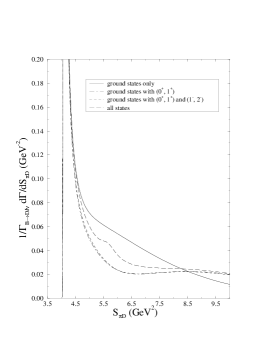
FIG. 2.: $\frac{1}{\Gamma(B\rightarrow D\ell\nu)}\,\frac{\partial\Gamma_{B_{\ell 4}}}{\partial S_{D\pi}}$ as a function of $S_{D\pi}$ for $B\to D\pi^{\pm}e\nu$. The different curves correspond to different combinations of resonances, as explained in the figure.

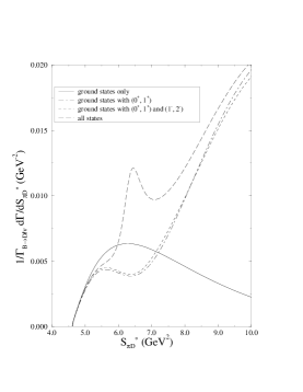
FIG. 3.: $\frac{1}{\Gamma(B\rightarrow D\ell\nu)}\,\frac{\partial\Gamma_{B_{\ell 4}}}{\partial S_{D\pi}}$ as a function of $S_{D\pi}$ for $B\to D^{*}\pi^{\pm}e\nu$.

Figures 2 and 3 show the spectra for the decays $B\to D\pi\ell\nu$ and $B\to D^{*}\pi\ell\nu$, respectively. Each of these figures shows four curves, corresponding to the inclusion of various combinations of multiplets in the analysis. One very interesting feature in these spectra is the narrow structure due to the $(0^{-},1^{-})^{\prime}$ $D$ meson multiplet. We will discuss this feature in some more detail later. Another notable feature is the depletion in the differential and total widths of $B\to D\pi\ell\nu$ that arises from the interference between the $(0^{-},1^{-})$ and $(0^{+},1^{+})$ multiplets. In the case of the decay $B\to D^{*}\pi\ell\nu$, the depletion caused by this interference at values of $S_{D^{*}\pi}\leq 8.5$ GeV² is more than compensated by the enhancement that occurs throughout the rest of phase space. This latter enhancement should however be taken with caution, as it lies beyond the range of applicability of our approximation.

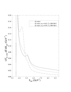
FIG. 4.: The effect on the decay $B\to D\pi^{\pm}e\nu$, of changing the couplings and total widths of the states in the $(0^{+},1^{+})$ multiplet.

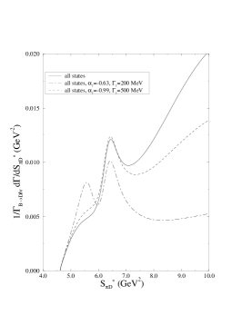
FIG. 5.: The effect on the decay $B\to D^{*}\pi^{\pm}e\nu$, of changing the couplings and total widths of the states in the $(0^{+},1^{+})$ multiplet.

In figures 4 to 7 we examine the effects of the values of some of the parameters on the spectra. Figures 4 and 5 show the effect of changing the coupling constant and width of the states in the $(0^{+},1^{+})$ multiplet. The values we have obtained in our model are $\alpha_{1}=-1.43~{}(-1.22)$ and $\Gamma=1.04~{}(0.756)$ GeV. This width may seem very large, but it is at least consistent with other model calculations. Nevertheless, we have investigated the effect of using smaller widths, namely 500 MeV and 200 MeV. $\alpha_{1}$ is changed to -0.99 and -0.63, respectively, in keeping with these changes. We see that the effect on the spectrum of $B\to D\pi\ell\nu$ is quite striking, especially at the narrower of the two widths. The effect on the spectrum of $B\to D^{*}\pi\ell\nu$ is similarly striking. The total width of the $B\to D^{*}\pi\ell\nu$ decay is strongly affected by these changes, changing from $1.7~{}(1.7)\times 10^{-15}$ GeV to $1.0~{}(1.2)\times 10^{-15}$ GeV and $4.9~{}(5.9)\times 10^{-16}$ GeV as the total width of this multiplet changes from 1.04  (0.756) GeV to 500 MeV to 200 MeV. In comparison, the total width of $B\to D\pi\ell\nu$ is essentially unaffected by these changes.

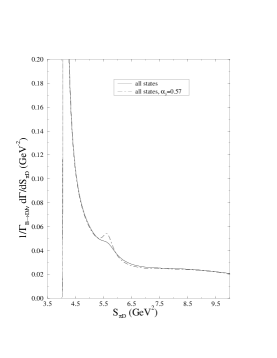
FIG. 6.: The effect on the decay $B\to D\pi^{\pm}e\nu$, of changing the couplings and total widths of the states in the $(0^{-},1^{-})^{\prime}$ multiplet.

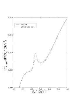
FIG. 7.: The effect on the decay $B\to D^{*}\pi^{\pm}e\nu$, of changing the couplings and total widths of the states in the $(0^{-},1^{-})^{\prime}$ multiplet.

In figures 6 and 7 we illustrate the effect of changing the total width of the $(0^{-},1^{-})^{\prime}$ multiplet from 191  (174) MeV to 130 MeV, accompanied by a change in $\alpha_{3}$ from 0.69  (0.66) to 0.57. We see that the narrower state would provide a clearer signal for experimentalists. The possibility of observing this pair of states in $B_{\ell 4}$ decays will depend strongly on the value of the total width and on $\alpha_{3}$, as well as on the effects that various experimental cuts will have on the spectra we illustrate. While we do not study the effects of cuts in this work, we can estimate the number of events that one may see in the proposed $B$-factory.

The integrated width under the peak (from about 5.33 to 6.0 GeV²) is $2.7~{}(3.9)\times 10^{-16}$ GeV, corresponding to a branching fraction of $5.2~{}(7.4)\times 10^{-4}$, or about $5.2~{}(7.4)\times 10^{4}$ events, assuming production of $10^{8}$ $B$ mesons. Subtracting the width that corresponds to a ‘smooth’ background leaves $220~{}(7000)$ events in the peak alone. A similar exercise in the case of the $D^{*}\pi\ell\nu$ spectrum yields a width of $7.4~{}(10.3)\times 10^{-17}$ GeV, corresponding to 14200 (19900) events. Removing the smooth background leaves 1800 (4300) events in the resonant peak.

While the dependence on the model parameters is clear, these estimates suggest that a study of the spectra of $B\to D\pi\ell\nu$ and $B\to D^{*}\pi\ell\nu$ offer some opportunity for discovery or confirmation of the resonances of the $(0^{-},1^{-})^{\prime}$ multiplet. Note that if we include the expected small mass difference between these two states, the single peak in these figures will become two peaks that are very close together (separated by about 0.32 GeV² if the mass splitting is about 60 MeV). The net effect would be a broadening of the structure that we have in our spectra.

In conclusion, we have studied $B_{\ell 4}$ decays in the soft-pion limit using chiral perturbation theory and heavy quark symmetry. The resonances which give leading contributions in this limit have been included, and shown to be important in determining both the rate and the shape of the spectrum. The narrow $(0^{-},1^{-})^{\prime}$ resonances show up as a peak in the $S_{D\pi}$ spectrum, and will likely be difficult to observe in $B\to D\pi\ell\nu$. The possibility for detection or confirmation in $B\to D^{*}\pi\ell\nu$ is more promising. The wider resonances of the $(0^{+},1^{+})$ multiplet show some effect on the total rate, but are not likely to be identified from the spectrum. Preliminary indications are that they may be identified at Aleph using the topology of the $B_{\ell 4}$ decays [21]. The effect of these broad resonances is much more pronounced for $B\to D^{*}\pi\ell\nu$ than for $B\to D\pi\ell\nu$, although the effects on both spectra are quite clear.

A Strong interaction transition vertices with a single pion

FIG. 8.: Vertices obtained from the chiral Lagrangian for soft neutral pion emission. Vertices for charged pion emission are a factor $\sqrt{2}$ of those shown in this figure.

In this appendix, we give the explicit expressions for the vertices where one pion emission takes place according to ${\cal L}_{\chi}^{\rm int}$. Similar results hold for B mesons. The vertices are shown in figure 8.

B The charged currents

In this appendix the explicit expressions for the charged currents displayed in eq. (25) are presented. They are

$$J_{\mu}(0^{-}\rightarrow 0^{-}) = -\xi(\nu)\,D^{\dagger}(v^{\prime})(v+v^{\prime})_{\mu}B(v),$$ (B1)

$$J_{\mu}(0^{-}\rightarrow 1^{-}) = \xi(\nu)\,D^{\ast\dagger\nu}(v^{\prime})\left[i\epsilon_{\nu\mu\alpha\beta}v^{\prime\alpha}v^{\beta}+g_{\mu\nu}(1+\nu)-v^{\prime}_{\mu}v_{\nu}\right]B(v),$$ (B2)

$$J_{\mu}(1^{-}\rightarrow 0^{-}) = \xi(\nu)\,D^{\dagger}(v^{\prime})\left[i\epsilon_{\mu\alpha\beta\rho}v^{\alpha}v^{\prime\beta}+g_{\mu\rho}(1+\nu)-v_{\mu}v^{\prime}_{\rho}\right]B^{\ast\rho}(v),$$ (B3)

$$J_{\mu}(1^{-}\rightarrow 1^{-}) = \xi(\nu)\,D^{\ast\dagger\nu}(v^{\prime})$$ (B4)

$$\times \left[g_{\nu\rho}(v+v^{\prime})_{\mu}-g_{\mu\rho}v_{\nu}-g_{\mu\nu}v^{\prime}_{\rho}+i\epsilon_{\mu\alpha\rho\nu}(v+v^{\prime})^{\alpha}\right]B^{\ast\rho}(v),$$ (B5)

$$J_{\mu}(0^{-}\rightarrow 0^{+}) = -\rho_{1}(\nu)\;D_{+}^{\dagger}(v^{\prime})(v-v^{\prime})_{\mu}B(v),$$ (B6)

$$J_{\mu}(0^{-}\rightarrow 1^{+}) = \rho_{1}(\nu)\;D_{+}^{\ast\dagger\nu}(v^{\prime})\left[i\epsilon_{\mu\nu\alpha\beta}v^{\alpha}v^{\prime\beta}+g_{\mu\nu}(\nu-1)-v^{\prime}_{\mu}v_{\nu}\right]B(v),$$ (B7)

$$J_{\mu}(1^{-}\rightarrow 0^{+}) = \rho_{1}(\nu)\;D_{+}^{\dagger}(v^{\prime})\left[-i\epsilon_{\mu\alpha\beta\rho}v^{\alpha}v^{\prime\beta}-g_{\mu\rho}(\nu-1)+v_{\mu}v^{\prime}_{\rho}\right]B^{\ast\rho}(v),$$ (B8)

$$J_{\mu}(1^{-}\rightarrow 1^{+}) = \rho_{1}(\nu)\;D_{+}^{\ast\dagger\nu}(v^{\prime})$$ (B9)

$$\times \left[-g_{\nu\rho}(v-v^{\prime})_{\mu}+g_{\mu\rho}v_{\nu}-g_{\mu\nu}v^{\prime}_{\rho}+i\epsilon_{\nu\mu\rho\alpha}(-v+v^{\prime})^{\alpha}\right]B^{\ast\rho}(v),$$ (B10)

$$J_{\mu}(0^{-}\rightarrow 1^{-}) = \frac{1}{\sqrt{6}}\rho_{2}(\nu)\,D_{1^{-}}^{\dagger\nu}(v^{\prime})$$ (B11)

$$\times \left[i\epsilon_{\mu\nu\alpha\beta}v^{\alpha}v^{\prime\beta}(\nu-1)+g_{\mu\nu}(\nu^{2}-1)-v_{\nu}((2+\nu)v^{\prime}_{\mu}-3v_{\nu})\right]B(v),$$ (B12)

$$J_{\mu}(0^{-}\rightarrow 2^{-}) = -\rho_{2}(\nu)\,D_{2^{-}}^{\ast\dagger\nu\rho}(v^{\prime})$$ (B13)

$$\times \left[-v_{\nu}g_{\mu\rho}(\nu-1)+v_{\nu}v_{\rho}v^{\prime}_{\mu}+i\epsilon_{\mu\nu\alpha\beta}v_{\rho}v^{\alpha}v^{\prime\beta}\right]B^{\ast\sigma}(v),$$ (B14)

$$J_{\mu}(1^{-}\rightarrow 1^{-}) = \frac{1}{\sqrt{6}}\rho_{2}(\nu)\,D_{1^{-}}^{\dagger\nu}(v^{\prime})$$ (B15)

$$\times \left[(v+v^{\prime})_{\mu}g_{\nu\sigma}(\nu-1)-3v_{\nu}v_{\mu}v^{\prime}_{\sigma}+2v_{\nu}g_{\mu\sigma}(\nu-1)-g_{\mu\nu}v^{\prime}_{\sigma}(\nu-1)\right.$$ (B16)

$$- \left.i\epsilon_{\mu\nu\alpha\sigma}(v-v^{\prime})^{\alpha}(1+\nu)+2i\epsilon_{\nu\sigma\alpha\beta}v^{\alpha}v_{\mu}v^{\prime\beta}+i\epsilon_{\mu\sigma\alpha\beta}v_{\nu}v^{\alpha}v^{\prime\beta}\right]B^{\ast\sigma}(v),$$ (B17)

$$J_{\mu}(1^{-}\rightarrow 2^{-}) = \rho_{2}(\nu)\,D_{2^{-}}^{\ast\dagger\nu\rho}(v^{\prime})$$ (B18)

$$\times \left[-i\epsilon_{\mu\nu\delta\sigma}v_{\rho}(v-v^{\prime})^{\delta}+g_{\mu\sigma}v_{\nu}v_{\rho}-g_{\mu\rho}v_{\nu}v^{\prime}_{\sigma}-g_{\rho\sigma}v_{\nu}(v-v^{\prime})_{\mu}\right]B^{\ast\sigma}(v),$$ (B19)

$$J_{\mu}(0^{-}\rightarrow 0^{-\prime}) = -\xi^{(1)}(\nu)\,D^{\prime\dagger}(v^{\prime})(v+v^{\prime})_{\mu}B(v),$$ (B20)

$$J_{\mu}(0^{-}\rightarrow 1^{-\prime}) = \xi^{(1)}(\nu)\,D^{\prime\ast\dagger\nu}(v^{\prime})\left[i\epsilon_{\nu\mu\alpha\beta}v^{\prime\alpha}v^{\beta}+g_{\mu\nu}(1+\nu)-v^{\prime}_{\mu}v_{\nu}\right]B(v),$$ (B21)

$$J_{\mu}(1^{-}\rightarrow 0^{-\prime}) = \xi^{(1)}(\nu)\,D^{\prime\dagger}(v^{\prime})\left[i\epsilon_{\mu\alpha\beta\rho}v^{\alpha}v^{\prime\beta}+g_{\mu\rho}(1+\nu)-v_{\mu}v^{\prime}_{\rho}\right]B^{\ast\rho}(v),$$ (B22)

$$J_{\mu}(1^{-}\rightarrow 1^{-\prime}) = \xi^{(1)}(\nu)\,D^{\prime\ast\dagger\nu}(v^{\prime})$$ (B23)

$$\times \left[g_{\nu\rho}(v+v^{\prime})_{\mu}-g_{\mu\rho}v_{\nu}-g_{\mu\nu}v^{\prime}_{\rho}+i\epsilon_{\mu\alpha\rho\nu}(v+v^{\prime})^{\alpha}\right]B^{\ast\rho}(v).$$ (B24)

The effective currents where a $B$-meson resonance decays into a ground state $D$-meson are easily obtained simply taking the hermitian (minus the hermitian) conjugate of the vector (axial-vector) portion of the currents displayed above followed by the interchange of symbols $B\leftrightarrow D$ and $v\leftrightarrow v^{\prime}$.

C The Form Factors

In this appendix we give the form factors needed in eqns. ( 73) and (108). The non-resonant and the resonant contributions are displayed separately.

1 $B\rightarrow D\pi\ell\bar{\nu}$

If we write

$$\Omega_{\mu}=-ih\;M_{B}M_{D}\,\epsilon_{\mu\nu\rho\sigma}v^{\nu}v^{\prime\rho}p_{\pi}^{\sigma}+A_{1}\;p_{\pi\mu}+A_{2}\;M_{B}v_{\mu}+A_{3}\;M_{D}v^{\prime}_{\mu},$$ (C1)

the form factors in equation (73) are

$$H = -h,$$ (C2)

$$F = A_{2}+\frac{1}{2}(A_{1}+A_{3}),$$ (C3)

$$G = \frac{1}{2}(A_{3}-A_{1}),$$ (C4)

$$R = A_{2}.$$ (C5)

From eqn. (43) we obtain the non-resonant contributions to the form factors as

$$h_{NR} = \frac{g}{2F_{0}}\;\frac{\xi(\nu)}{M_{B}M_{D}}\;\left(\frac{1}{p_{\pi}\!\cdot\!v+\delta m_{B}-i\epsilon}-\frac{1}{p_{\pi}\!\cdot\!v^{\prime}-\delta m_{D}+i\epsilon}\right),$$ (C6)

$$A_{1\,NR} = -\frac{g}{2F_{0}}\;\xi(\nu)\;(1+\nu)\left(\frac{1}{p_{\pi}\!\cdot\!v+\delta m_{B}-i\epsilon}-\frac{1}{p_{\pi}\!\cdot\!v^{\prime}-\delta m_{D}+i\epsilon}\right),$$ (C7)

$$A_{2\,NR} = \frac{g}{2F_{0}}\;\frac{\xi(\nu)}{M_{B}}\;\left(\frac{p_{\pi}\!\cdot\!v+p_{\pi}\!\cdot\!v^{\prime}}{p_{\pi}\!\cdot\!v+\delta m_{B}-i\epsilon}\right),$$ (C8)

$$A_{3\,NR} = -\frac{g}{2F_{0}}\;\frac{\xi(\nu)}{M_{D}}\left(\frac{p_{\pi}\!\cdot\!v+p_{\pi}\!\cdot\!v^{\prime}}{p_{\pi}\!\cdot\!v^{\prime}-\delta m_{D}+i\epsilon}\right).$$ (C9)

These results are the same as those obtained by Lee and collaborators [7], and by Cheng and collaborators [8].

FIG. 9.: Non-resonant (a) and resonant (b) diagrams contributing to $B\rightarrow D\pi\ell\bar{\nu}$. The dashed line represents the pion and the dotted line which emerges from the electroweak charged current carries the momentum of the $\ell\bar{\nu}$ pair. Horizontal solid lines correspond to four velocity $v$ and the oblique ones to $v^{\prime}$.

From eqn. (46) the resonant contributions are

$$h_{R} = \frac{\alpha_{2}\;\rho_{2}(\nu)}{6F_{0}M_{B}M_{D}}\;\,(\nu-1)\left(\frac{1}{p_{\pi}\!\cdot\!v+\delta\tilde{m}_{2}}-\frac{1}{p_{\pi}\!\cdot\!v^{\prime}-\delta\tilde{m}_{2}}\right)$$ (C10)

$$+ \frac{\alpha_{3}}{2F_{0}}\;\frac{\xi^{(1)}(\nu)}{M_{B}M_{D}}\;\left(\frac{1}{p_{\pi}\!\cdot\!v+\delta\tilde{m}_{3}}-\frac{1}{p_{\pi}\!\cdot\!v^{\prime}-\delta\tilde{m}_{3}}\right),$$ (C11)

$$A_{1\,R} = -\frac{\alpha_{2}\;\rho_{2}(\nu)}{6F_{0}}\;(\nu^{2}-1)\;\left(\frac{1}{p_{\pi}\!\cdot\!v+\delta\tilde{m}_{2}}-\frac{1}{p_{\pi}\!\cdot\!v^{\prime}-\delta\tilde{m}_{2}}\right)$$ (C12)

$$- \frac{\alpha_{3}\,\xi^{(1)}(\nu)}{2F_{0}}\;(1+\nu)\left(\frac{1}{p_{\pi}\!\cdot\!v+\delta\tilde{m}_{3}}-\frac{1}{p_{\pi}\!\cdot\!v^{\prime}-\delta\tilde{m}_{3}}\right),$$ (C13)

$$A_{2\,R} = \frac{\alpha_{1}\;\rho_{1}(\nu)}{2F_{0}M_{B}}\left(\frac{p_{\pi}\!\cdot\!v^{\prime}}{p_{\pi}\!\cdot\!v^{\prime}-\delta\tilde{m}_{1}}+\frac{p_{\pi}\!\cdot\!v}{p_{\pi}\!\cdot\!v+\delta\tilde{m}_{1}}\right)$$ (C14)

$$+ \frac{\alpha_{2}\;\rho_{2}(\nu)}{F_{0}M_{B}}\;\left\{\frac{1}{p_{\pi}\!\cdot\!v+\delta\tilde{m}_{2}}\left[\frac{1}{6}(\nu\;p_{\pi}\!\cdot\!v^{\prime}-p_{\pi}\!\cdot\!v)+\frac{1}{3}(p_{\pi}\!\cdot\!v^{\prime}-\nu\;p_{\pi}\!\cdot\!v)\right]\right.$$ (C15)

$$+ \left.\frac{1}{2}\frac{1}{p_{\pi}\!\cdot\!v^{\prime}-\delta\tilde{m}_{2}}(p_{\pi}\!\cdot\!v-\nu\;p_{\pi}\!\cdot\!v^{\prime})\right\}$$ (C16)

$$+ \frac{\alpha_{3}}{2F_{0}}\;\frac{\xi^{(1)}(\nu)}{M_{B}}\;\left(\frac{p_{\pi}\!\cdot\!(v+v^{\prime})}{p_{\pi}\!\cdot\!v+\delta\tilde{m}_{3}}\right),$$ (C17)

$$A_{3\,R} = -\frac{\alpha_{1}\;\rho_{1}(\nu)}{2F_{0}M_{D}}\left(\frac{p_{\pi}\!\cdot\!v^{\prime}}{p_{\pi}\!\cdot\!v^{\prime}-\delta\tilde{m}_{1}}+\frac{p_{\pi}\!\cdot\!v}{p_{\pi}\!\cdot\!v+\delta\tilde{m}_{1}}\right)$$ (C18)

$$- \frac{\alpha_{2}\;\rho_{2}(\nu)}{F_{0}M_{D}}\;\left\{\frac{1}{p_{\pi}\!\cdot\!v^{\prime}-\delta\tilde{m}_{2}}\left[\frac{1}{6}(\nu\;p_{\pi}\!\cdot\!v-p_{\pi}\!\cdot\!v^{\prime})+\frac{1}{3}(p_{\pi}\!\cdot\!v-\nu\;p_{\pi}\!\cdot\!v^{\prime})\right]\right.$$ (C19)

$$+ \left.\frac{1}{2}\;\frac{1}{p_{\pi}\!\cdot\!v+\delta\tilde{m}_{2}}(p_{\pi}\!\cdot\!v^{\prime}-\nu\;p_{\pi}\!\cdot\!v)\right\}$$ (C20)

$$- \frac{\alpha_{3}}{2F_{0}}\;\frac{\xi^{(1)}(\nu)}{M_{D}}\;\left(\frac{p_{\pi}\!\cdot\!(v+v^{\prime})}{p_{\pi}\!\cdot\!v^{\prime}-\delta\tilde{m}_{3}}\right).$$ (C21)

2 $B\rightarrow D^{\ast}\pi\ell\nu$

The most general form for the tensor $\Omega_{\mu\nu}$ in terms of the vectors $v_{\mu}$, $v_{\mu}^{\prime}$ and $p_{\pi\mu}$ is (terms which vanish upon contraction with $\epsilon^{\ast\nu}_{D}(v^{\prime})$ are not displayed)

$$\Omega_{\mu\nu}(v,v^{\prime},p_{\pi}) = \frac{i}{2}\;\epsilon_{\mu\nu\rho\sigma}\;\left[h_{1}\;M_{B}M_{D}v^{\rho}v^{\prime\sigma}+h_{2}\;M_{B}v^{\rho}p_{\pi}^{\sigma}+h_{3}\;M_{D}v^{\prime\rho}p_{\pi}^{\sigma}\right]$$ (C22)

$$+ f_{1}\;M_{B}v_{\mu}p_{\pi\nu}+f_{2}\;M_{D}v^{\prime}_{\mu}p_{\pi\nu}+f_{3}\;p_{\pi\mu}p_{\pi\nu}+f_{4}\;M_{B}^{2}v_{\mu}v_{\nu}$$ (C23)

$$+ f_{5}\;M_{B}M_{D}v^{\prime}_{\mu}v_{\nu}+f_{6}\;M_{B}p_{\pi\mu}v_{\nu}+k\;g_{\mu\nu}$$ (C24)

$$+ \frac{i}{2}\;\epsilon_{\mu\delta\rho\sigma}\;v^{\delta}v^{\prime\rho}p_{\pi}^{\sigma}\;\left(g_{1}\;p_{\pi\nu}+g_{2}\;M_{B}v_{\nu}\right)$$ (C25)

$$+ \frac{i}{2}\;\epsilon_{\nu\delta\rho\sigma}\;v^{\delta}v^{\prime\rho}p_{\pi}^{\sigma}\;\left(g_{3}\;M_{B}v_{\mu}+g_{4}\;M_{D}v^{\prime}_{\mu}+g_{5}\;p_{\pi\mu}\right).$$ (C26)

The form factors appearing in eqn. (108) are related to the ones in this expression by

$$H_{1} = \frac{1}{2}\;(h_{1}-h_{2}-h_{3}),$$ (C27)

$$H_{2} = -\frac{1}{2}\;(h_{1}+h_{2}),$$ (C28)

$$H_{3} = \frac{1}{2}\;(-h_{1}+h_{2}),$$ (C29)

$$F_{1} = \frac{1}{2}\;\left(f_{1}+f_{2}+\frac{1}{2}f_{3}+f_{4}+\frac{1}{2}f_{5}+\frac{1}{2}f_{6}\right),$$ (C30)

$$F_{2} = \frac{1}{4}\;\left(f_{2}-f_{3}+f_{5}-f_{6}\right),$$ (C31)

$$F_{3} = f_{4}+\frac{1}{2}\;(f_{5}+f_{6}),$$ (C32)

$$F_{4} = \frac{1}{2}\;(f_{5}-f_{6}),$$ (C33)

$$K = k,$$ (C34)

$$G^{A}_{1} = -\frac{1}{4M_{B}M_{D}}\;(g_{1}+g_{2}),$$ (C35)

$$G^{A}_{2} = -\frac{1}{2M_{B}M_{D}}g_{2},$$ (C36)

$$G^{B}_{1} = -\frac{1}{2M_{B}M_{D}}\;\left(g_{3}+\frac{1}{2}\;(g_{4}+g_{5})\right),$$ (C37)

$$G^{B}_{2} = -\frac{1}{4M_{B}M_{D}}\;(g_{4}-g_{5}).$$ (C38)

FIG. 10.: Non-resonant (a) and resonant (b) diagrams contributing to $B\rightarrow D^{\ast}\pi\ell\bar{\nu}$.

From eqn. (54) the non-resonant contributions to the form factors are

$$h_{1\,NR} = -\frac{g\xi(\nu)}{F_{0}M_{B}M_{D}}\;\;\frac{p_{\pi}\!\cdot\!v}{p_{\pi}\!\cdot\!v+\delta m_{B}-i\epsilon},$$ (C39)

$$h_{2\,NR} = -\frac{g\xi(\nu)}{F_{0}M_{B}}\;\;\frac{1}{p_{\pi}\!\cdot\!v+\delta m_{B}-i\epsilon},$$ (C40)

$$h_{3\,NR} = -\frac{g\xi(\nu)}{F_{0}M_{D}}\;\left(\frac{1}{p_{\pi}\!\cdot\!v+\delta m_{B}-i\epsilon}-\frac{1+\nu}{p_{\pi}\!\cdot\!v^{\prime}+i\epsilon}\right),$$ (C41)

$$f_{1\,NR} = -\frac{g\xi(\nu)}{2F_{0}M_{B}}\;\left(\frac{1}{p_{\pi}\!\cdot\!v+\delta m_{B}-i\epsilon}-\frac{1}{p_{\pi}\!\cdot\!v^{\prime}+\delta m_{D}+i\epsilon}\right),$$ (C42)

$$f_{2\,NR} = \frac{M_{B}}{M_{D}}\;f_{1\,NR},$$ (C43)

$$f_{3\,NR} = f_{4\,NR}=0,$$ (C44)

$$f_{5\,NR} = \frac{g\xi(\nu)}{2F_{0}M_{B}M_{D}}\,\left(1+\frac{p_{\pi}\!\cdot\!v}{p_{\pi}\!\cdot\!v+\delta m_{B}-i\epsilon}\right),$$ (C45)

$$f_{6\,NR} = \frac{g\xi(\nu)}{2F_{0}M_{B}}\;\left(\frac{1}{p_{\pi}\!\cdot\!v+\delta m_{B}-i\epsilon}-\frac{1}{p_{\pi}\!\cdot\!v^{\prime}+i\epsilon}\right),$$ (C46)

$$k_{NR} = \frac{g\xi(\nu)}{2\,F_{0}}\;\left(\frac{p_{\pi}\!\cdot\!v^{\prime}-\nu\,p_{\pi}\!\cdot\!v}{p_{\pi}\!\cdot\!v+\delta m_{B}-i\epsilon}+\frac{p_{\pi}\!\cdot\!v-\nu\,p_{\pi}\!\cdot\!v^{\prime}}{p_{\pi}\!\cdot\!v^{\prime}+i\epsilon}\right),$$ (C47)

$$g_{1\,NR} = 0,$$ (C48)

$$g_{2\,NR} = 0,$$ (C49)

$$g_{3\,NR} = 0,$$ (C50)

$$g_{4\,NR} = \frac{g\xi(\nu)}{F_{0}\,M_{D}}\;\;\frac{1}{\,p_{\pi}\!\cdot\!v^{\prime}+i\epsilon},$$ (C51)

$$g_{5\,NR} = 0.$$ (C52)

These results are the same as those obtained by other authors [7, 8].

Finally, the resonant contributions are obtained from eqn. ( 57) and are

$$h_{1\,R} = \frac{\alpha_{1}\;\rho_{1}(\nu)}{F_{0}M_{B}M_{D}}\;\left(\frac{p_{\pi}\!\cdot\!v}{-p_{\pi}\!\cdot\!v-\delta\tilde{m}_{1}}-\frac{p_{\pi}\!\cdot\!v^{\prime}}{p_{\pi}\!\cdot\!v^{\prime}-\delta\tilde{m}_{1}}\right)$$ (C53)

$$+ \frac{\alpha_{2}\;\rho_{2}(\nu)}{3F_{0}M_{B}M_{D}}\;\left(\frac{p_{\pi}\!\cdot\!v\,(1+2\nu)-p_{\pi}\!\cdot\!v^{\prime}}{p_{\pi}\!\cdot\!v+\delta\tilde{m}_{2}}+\frac{3}{2}\frac{\nu\;p_{\pi}\!\cdot\!v^{\prime}-p_{\pi}\!\cdot\!v}{p_{\pi}\!\cdot\!v^{\prime}-\delta\tilde{m}_{2}}\right)$$ (C54)

$$- \frac{\alpha_{3}\;\xi^{(1)}(\nu)}{F_{0}M_{B}M_{D}}\frac{p_{\pi}\!\cdot\!v}{p_{\pi}\!\cdot\!v+\delta\tilde{m}_{3}},$$ (C55)

$$h_{2\,R} = \frac{\alpha_{2}\;(1+\nu)\;\rho_{2}(\nu)}{3F_{0}M_{B}}\frac{1}{-p_{\pi}\!\cdot\!v-\delta\tilde{m}_{2}}-\frac{\alpha_{3}\;\xi^{(1)}(\nu)}{F_{0}M_{B}\;(p_{\pi}\!\cdot\!v+\delta\tilde{m}_{3})},$$ (C56)

$$h_{3\,R} = \frac{\alpha_{2}\;\rho_{2}(\nu)}{3F_{0}M_{D}}\;\left(\frac{1+\nu}{p_{\pi}\!\cdot\!v+\delta\tilde{m}_{2}}-\frac{\nu^{2}-1}{2(p_{\pi}\!\cdot\!v^{\prime}-\delta\tilde{m}_{2})}\right)$$ (C57)

$$- \frac{\alpha_{3}\;\xi^{(1)}(\nu)}{F_{0}M_{D}}\;\left(\frac{1}{p_{\pi}\!\cdot\!v+\delta\tilde{m}_{3}}-\frac{1+\nu}{p_{\pi}\!\cdot\!v^{\prime}-\delta\tilde{m}_{3}}\right),$$ (C58)

$$f_{1\,R} = -\frac{\alpha_{2}\;\rho_{2}(\nu)\,(\nu-1)}{6F_{0}M_{B}}\;\left(\frac{1}{p_{\pi}\!\cdot\!v+\delta\tilde{m}_{2}}-\frac{1}{p_{\pi}\!\cdot\!v^{\prime}-\delta\tilde{m}_{2}}\right)$$ (C59)

$$- \frac{\alpha_{3}\;\xi^{(1)}(\nu)}{2F_{0}M_{B}}\;\left(\frac{1}{p_{\pi}\!\cdot\!v+\delta\tilde{m}_{3}}-\frac{1}{p_{\pi}\!\cdot\!v^{\prime}-\delta\tilde{m}_{3}}\right),$$ (C60)

$$f_{2\,R} = \frac{M_{B}}{M_{D}}\;f_{1\,R},$$ (C61)

$$f_{3\,R} = f_{4\,R}=0,$$ (C62)

$$f_{5\,R} = \frac{\alpha_{1}\;\rho_{1}(\nu)}{2F_{0}M_{B}M_{D}}\;\left(\frac{p_{\pi}\!\cdot\!v}{p_{\pi}\!\cdot\!v+\delta\tilde{m}_{1}}+\frac{p_{\pi}\!\cdot\!v^{\prime}}{p_{\pi}\!\cdot\!v^{\prime}-\delta\tilde{m}_{1}}\right)$$ (C63)

$$+ \frac{\alpha_{2}\;\rho_{2}(\nu)}{2F_{0}M_{B}M_{D}}\;\left(\frac{p_{\pi}\!\cdot\!v^{\prime}-\frac{1}{3}p_{\pi}\!\cdot\!v\,(1+2\,\nu)}{p_{\pi}\!\cdot\!v+\delta\tilde{m}_{2}}+\frac{p_{\pi}\!\cdot\!v-\frac{1}{3}p_{\pi}\!\cdot\!v^{\prime}\,(1+2\,\nu)}{p_{\pi}\!\cdot\!v^{\prime}-\delta\tilde{m}_{2}}\right)$$ (C64)

$$+ \frac{\alpha_{3}\;\xi^{(1)}(\nu)}{2F_{0}M_{B}M_{D}}\;\left(\frac{p_{\pi}\!\cdot\!v}{p_{\pi}\!\cdot\!v+\delta\tilde{m}_{3}}+\frac{p_{\pi}\!\cdot\!v^{\prime}}{p_{\pi}\!\cdot\!v^{\prime}-\delta\tilde{m}_{3}}\right),$$ (C65)

$$f_{6\,R} = \frac{\alpha_{2}\;\rho_{2}(\nu)\,(\nu-1)}{6F_{0}M_{B}}\;\left(\frac{1}{p_{\pi}\!\cdot\!v+\delta\tilde{m}_{2}}-\frac{1}{p_{\pi}\!\cdot\!v^{\prime}-\delta\tilde{m}_{2}}\right)$$ (C66)

$$+ \frac{\alpha_{3}\;\xi^{(1)}(\nu)}{2F_{0}M_{B}}\;\left(\frac{1}{p_{\pi}\!\cdot\!v+\delta\tilde{m}_{3}}-\frac{1}{p_{\pi}\!\cdot\!v^{\prime}-\delta\tilde{m}_{3}}\right),$$ (C67)

$$k_{R} = -\frac{\alpha_{1}\;\rho_{1}(\nu)\,(\nu-1)}{2F_{0}}\;\left(\frac{p_{\pi}\!\cdot\!v}{p_{\pi}\!\cdot\!v+\delta\tilde{m}_{1}}+\frac{p_{\pi}\!\cdot\!v^{\prime}}{p_{\pi}\!\cdot\!v^{\prime}-\delta\tilde{m}_{1}}\right)$$ (C68)

$$- \frac{\alpha_{2}\;\rho_{2}(\nu)\,(\nu-1)}{3F_{0}}\;\left(\frac{(p_{\pi}\!\cdot\!v^{\prime}-\nu\;p_{\pi}\!\cdot\!v)}{p_{\pi}\!\cdot\!v+\delta\tilde{m}_{2}}+\frac{(p_{\pi}\!\cdot\!v-\nu\;p_{\pi}\!\cdot\!v^{\prime})}{p_{\pi}\!\cdot\!v^{\prime}-\delta\tilde{m}_{2}}\right)$$ (C69)

$$+ \frac{\alpha_{3}\;\xi^{(1)}(\nu)}{2F_{0}}\;\left(\frac{(p_{\pi}\!\cdot\!v^{\prime}-\nu\;p_{\pi}\!\cdot\!v)}{p_{\pi}\!\cdot\!v+\delta\tilde{m}_{3}}+\frac{(p_{\pi}\!\cdot\!v-\nu\;p_{\pi}\!\cdot\!v^{\prime})}{p_{\pi}\!\cdot\!v^{\prime}-\delta\tilde{m}_{3}}\right),$$ (C70)

$$g_{1\,R} = 0,$$ (C71)

$$g_{2\,R} = -\frac{\alpha_{2}\;\rho_{2}(\nu)}{2F_{0}\,M_{B}}\frac{1}{p_{\pi}\!\cdot\!v^{\prime}-\delta\tilde{m}_{2}},$$ (C72)

$$g_{3\,R} = -g_{2\,R},$$ (C73)

$$g_{4\,R} = \frac{\alpha_{2}\;\rho_{2}(\nu)}{3F_{0}\,M_{D}}\;\left(\frac{2}{p_{\pi}\!\cdot\!v+\delta\tilde{m}_{2}}-(1+\frac{1}{2}\,\nu)\frac{1}{p_{\pi}\!\cdot\!v^{\prime}-\delta\tilde{m}_{2}}\right)$$ (C74)

$$+ \frac{\alpha_{3}\;\xi^{(1)}(\nu)}{F_{0}}\frac{1}{p_{\pi}\!\cdot\!v^{\prime}-\delta\tilde{m}_{3}},$$ (C75)

$$g_{5\,R} = 0.$$ (C76)