QCD corrections to electroweak processes in an unconventional scheme: application to the $b\rightarrow s\gamma$ decay

Abstract

In this work we give a detailed description of a method for the calculation of QCD corrections to electroweak processes in dimensional regularization that does not require any definition of the $\gamma_{5}$ matrix in $d$ dimensions. This method appears particularly convenient in order to limit the algebraic complexity of higher order calculations. As an example, we compute the leading logarithmic corrections to the $b\rightarrow s\gamma$ decay.

IFUP-TH 9/94

HUTP-94/A001

, , and

^a Dipartimento di Fisica dell’Università di Pisa, Piazza Torricelli 2, I-56126 Pisa, ITALY, e-mail cella@sun10.difi.unipi.it 

^b Istituto Nazionale di Fisica Nucleare, Piazza Torricelli 2, I-56126 Pisa, ITALY, e-mail vicere@sun10.difi.unipi.it 

^c Lyman Laboratory of Physics, Harvard University, Cambridge, MA 02138, USA, e-mail ricciardi@physics.harvard.edu 

1 Introduction

In the Standard Model the flavor changing neutral current (FCNC) processes can take place only as loop effects because of the GIM mechanism. Therefore they are strongly suppressed compared with ordinary weak decays and very sensitive to the occurrence of new physics. Among all FCNC processes, the inclusive decay $B\rightarrow X_{s}\gamma$ is particularly interesting. In fact, due to the relatively heavy mass of the b-quark ($m_{b}\gg\mathchar 3\relax_{QCD}$), the long distance QCD contributions are expected to play a minor role and the process can be confidently modeled on the $b\rightarrow s\gamma$ decay in the spectator model, corrected for the short distance QCD corrections.

This approach has allowed a clean theoretical prediction of the inclusive rate, which is compatible with the recent experimental results from the CLEO collaboration [1, 2]. For instance at $m_{t}=174\pm 16\,{\mathrm{G}eV}$ [3] the theoretical prediction

$$BR\left[B\rightarrow X_{s}\gamma\right]_{\mathrm{t}heor}\pm\mathchar 1\relax_{\mathrm{t}heor}\pm\mathchar 1\relax_{m_{top}}=\left(3.0\pm 0.8\pm 0.1\right)\,10^{-4}$$ (1)

is larger than the exclusive fraction $B\rightarrow K^{\star}\gamma$

$$BR\left[B\rightarrow K^{\star}\,\gamma\right]=(4.5\pm 1.5\pm 0.9)\,10^{-5}$$ (2)

and smaller than the measured lower bound (at 95% confidence level) on the inclusive rate

$$BR[B\rightarrow X_{s}\,\gamma]<5.4\,10^{-4}.$$ (3)

Presently only the leading order QCD corrections (LO) are known. The importance of the next to leading order (NLO) corrections has been recently stressed by Buras et al. [4]. They have shown that most of the uncertainty in Eq. (1) comes from the residual dependence on the scale of the decay, and the inclusion of the subleading logarithms is a necessary step toward the reduction of the theoretical error, from about 25% to less than 10%.

It goes without saying that any search for new physics through the window of the rare $B$ decays is seriously hampered by so large an uncertainty in the Standard Model predictions. Since we expect that perturbative QCD works well at this scales of energy, at least for the inclusive predictions, the effort needed to reduce this uncertainty seems worthwhile.

In this paper we give full details about the computation of the LO corrections to $b\rightarrow s\gamma$ decay in dimensional regularization; the results of this work have already been published in [5]. We have applied to this problem a scheme that we consider an important step toward the computation of the NLO corrections and we want to substantiate the statement that this is a practical alternative to the t’Hooft-Veltman scheme, for this particular class of computations and in the context of dimensionally regularized field theory. To be definite, the method is helpful when evaluating the short distance corrections to a weak effective hamiltonian, induced by a theory that is invariant under the transformation $\gamma_{5}\rightarrow-\gamma_{5}$, like perturbative QCD. This scheme has been introduced in [6] and successfully applied to the NLO QCD corrections of a generic $\mathchar 1\relax F=1$ process in the absence of penguin operators.

Here we describe this method by applying it to the LO $b\rightarrow s\gamma$ computation. Our conclusions are that the latest LO existing results, obtained by Ciuchini et al. [7, 8], are correctly reproduced by this method and that it seems there are no technical obstructions to the computation of QCD corrections at all orders in perturbation theory.

We find useful to sketch here some major steps in the history of the LO corrections. The big enhancement of the decay rate due to QCD corrections was pointed out in [9, 10, 11], in the case of a light top quark. The first works where the top mass was considered sizable showed a substantial disagreement. In particular the more complete works of Grinstein et al. [12, 13, 14] and Grigjanis et al. [15, 16] seemed to show a contradiction between the naive dimensional regularization (NDR), based on the use of an anticommuting $\gamma_{5}$ matrix in $d$ dimensions and the method of dimensional reduction (DRED) [17].

This mismatch was practically very relevant: for example at $m_{t}=140\,\,\mathrm{GeV}$ the enhancement of the QCD corrected branching ratio was about a factor $4$ in the NDR scheme, to be compared with a factor $2$ in DRED.

In our work [18] we confirmed the result of the NDR analysis. All these computations were done in a reduced basis, not including certain operators whose contribution was supposed to be small [13].

The computation was extended to the complete basis by Misiak [19, 20]; the whole problem was reconsidered recently by Ciuchini et al. [7, 8], who have solved the contradiction between the NDR and DRED schemes demonstrating that the anomalous dimension (AD) matrix, even at leading logarithmic order, is scheme dependent. This scheme dependence is canceled in the physical amplitude just by the matrix elements of the operators left out in the first computations. Misiak has further observed in [21] that the scheme dependence could have been partly compensated in the reduced basis used by us in [18] by considering some matrix elements of operators related by the motion equations to the terms left out in the complete basis.

The results for the AD matrix reported in [7, 8] and in [20] are in slight disagreement, although this difference has little relevance on the phenomenology. In the present paper we confirm the AD matrix presented in [7, 8].

The plan of the paper is as follows: in Section 2 we describe the method on general grounds and we show that the computation of the anomalous dimension matrix can be considerably simplified by splitting the effective hamiltonian in parts even and odd under the $\gamma_{5}\rightarrow-\gamma_{5}$ transformation. After an extension of the $4$ dimensional operators to $d$ dimensions we can avoid the use of a $4$ dimensional $\gamma_{5}$, which is required in the t’Hooft-Veltman scheme [22], without any loss of mathematical rigor. In Section 3 we describe the computation of the QCD corrections to the $B\rightarrow X_{s}\gamma$ decay: while in our previous letter [5] we have given the results in an on-shell basis, here we consider useful to detail the work in an off-shell basis; the reason is that the intermediate results, although redundant, are useful for the planned next to leading computation. In section 4 we comment on the simplifications characteristics of this scheme, particularly the possibility to use generalized Fierz identities [23] to relate Feynman diagrams with and without fermionic traces: the existence of charge conjugation properties further reduces the number of independent graphs.

The appendixes are devoted to reference formulas: in App. A we list some results on the renormalization group in the context of dimensional regularization and we comment on the treatment of evanescent operators. In App. B we give a set of formulas needed to implement the Dirac algebra: they are known in literature, but we think useful to collect them in a “ready-to-use” form.

2 Strategy

In the following, we will explain our approach to the computation of the RG evolution. After reminding briefly the general framework for the computation of QCD corrections to weak decays, we will give full details about the symmetrized scheme we use [6].

The starting point is a “complete” theory of weak interactions and QCD, for instance the Standard Model, which enables us to predict amplitudes between initial and final states, at some order in perturbation theory

$$\left<f|i\right>_{\mathrm{complete}}.$$ (4)

It is well known that it is possible to simplify the computation of the amplitude in Eq. (4) building an effective hamiltonian ${\cal H}_{\mathrm{eff}}$ that models the effect of the degrees of freedom which are “heavy” compared to the typical energy scale of the process, in the sense that

$$\left<f|i\right>_{\mathrm{complete}}=\left<f\left|{\cal H}_{\mathrm{eff}}\right|i\right>_{\mathrm{light}}+O\left(\frac{1}{M^{4}}\right)\ ,$$ (5)

where $M$ is the “heavy” scale. ${\cal H}_{\mathrm{eff}}$ is a sum of local operators built of “light” fields. The dynamics is specified by a reduced lagrangian with the heavy fields deleted and with couplings and masses which undergo a finite renormalization while passing from the “complete” to the effective theory.

The effective hamiltonian is determined via a matching procedure: the operator content of ${\cal H}_{\mathrm{eff}}$ is obtained with considerations on the residual symmetries of the reduced lagrangian and the coefficients are computed imposing Eq. (5) on a finite number of processes. An important point is that, even when the “complete” theory is finite (for instance, when the divergences are canceled by the Glashow-Iliopoulos-Maiani mechanism), the effective hamiltonian contains operators, weighted with some inverse power of $M$, whose matrix elements are individually divergent and must be renormalized. A renormalization scale $\mu$ must therefore be introduced; we can write the effective hamiltonian as

$${\cal H}_{\mathrm{eff}}=\frac{1}{M^{2}}\sum_{i}C_{i}\left(\mu,\,M\right)N\left[{O_{i}}\right]\ ,$$ (6)

where the $N$ operation is a subtraction procedure, for instance minimal subtraction in dimensional regularization [24]. The matrix elements between on-shell states,

$$\left<f\left|N\left[{O_{i}}\right]\right|i\right>\left(\mu\simeq M\right)$$ (7)

contain large perturbative contributions depending on $\log{\mu/m}$, where $m$ is the typical scale of the external states. These large logarithms can be summed by exploiting the renormalization group invariance of the combination

$$\sum_{i}C_{i}\left(\mu,\,M\right)\left<f\left|N\left[{O_{i}}\right]\right|i\right>\left(\mu\right).$$ (8)

By scaling down the whole expression to values of $\mu\simeq m$, the large logarithms are transferred in the coefficients and the matrix elements can be computed more reliably.

The standard way to determine the RG evolution of the matrix elements is the computation of their anomalous dimension matrix $\hat{\gamma}$, which appears in the RG equation

$$\mu\frac{\,\mathrm{d}}{\,\mathrm{d}\mu}N\left[{O_{i}}\right]+\gamma_{ij}N\left[{O_{j}}\right]=0\ .$$ (9)

While the transition amplitude has physical meaning, the three steps of the computation, the matching at the $\mu\simeq M$ scale, the determination of the AD matrix and the evaluation of the matrix elements at the $\mu\simeq m$ scale, are in general all scheme dependent: we want to choose a framework which simplifies the most difficult part, the computation of the $\hat{\gamma}$ matrix.

2.1 An unconventional approach

Let us assume to have defined the effective theory in a regularization scheme free from ambiguities, like the t’Hooft-Veltman scheme, and to deal with a certain set of relevant operators, that is, operators with a non-zero naive limit in $4$-dimensions. They can also appear evanescent operators (classically zero in $4$-dimensions) that can be “reduced” on the relevant ones, and decoupled at the level of the RG evolution, as we shall see.

Let us consider the general structure of the effective hamiltonian, without specifying the field content

$${\cal H}_{\mathrm{eff}} = \sum_{i}C^{\mathrm{R,HV}}_{i}N\left[{R_{i}}\right]+\sum_{i}C^{\mathrm{L,HV}}_{i}N\left[{L_{i}}\right]$$ (10)

$$+ \sum_{i}C^{\mathrm{LL,HV}}_{i}N\left[{\left(L\otimes L\right)_{i}}\right]+\sum_{i}C^{\mathrm{LR,HV}}_{i}N\left[{\left(L\otimes R\right)_{i}}\right]\ .$$

The $N\left[{L}\right]$ and $N\left[{R}\right]$ operators are bilinear in the Fermi fields, like for instance $O_{2}$ and $O_{5}$ in the basis in Eq. (37), while $N\left[{L\otimes R}\right]$ and $N\left[{L\otimes L}\right]$ stand for current-current operators, like $O_{11}$ and $O_{13}$. The symbols $R$ and $L$ remind the presence of the chiral projectors $P_{\frac{L}{R}}=\frac{1}{2}(1\mp\gamma_{5})$, where $\gamma_{5}=-\gamma_{1}\gamma_{2}\gamma_{3}\gamma_{4}$ in euclidean notation. Now if we “redefine” the theory with the substitutions

$$\gamma_{5} \rightarrow \bar{\gamma}_{5}=-\gamma_{5}$$

$$\epsilon_{\mu\nu\rho\sigma} \rightarrow \bar{\epsilon}_{\mu\nu\rho\sigma}=-\epsilon_{\mu\nu\rho\sigma}$$ (11)

and compute the effective hamiltonian with the new Feynman rules (and the same regularization and renormalization scheme) we obtain an expression identical to the one in Eq. (10), except for the substitutions in Eq. (2.1). In fact, the commutation and trace rules are invariant under the transformation in Eq. (2.1), for example ($\tilde{\gamma}_{\mu}$ is the Dirac matrix in the $d-4$ unphysical space)

$$\left[\gamma_{\mu},\gamma_{5}\right]_{+}=2\gamma_{5}\tilde{\gamma}_{\mu} \rightarrow \left[\gamma_{\mu},\bar{\gamma}_{5}\right]_{+}=2\bar{\gamma}_{5}\tilde{\gamma}_{\mu}$$

$$\mathrm{Tr}\left(\gamma_{5}\gamma_{\mu}\gamma_{\nu}\gamma_{\rho}\gamma_{\sigma}\right)=4\epsilon_{\mu\nu\rho\sigma} \rightarrow \mathrm{Tr}\left(\bar{\gamma}_{5}\gamma_{\mu}\gamma_{\nu}\gamma_{\rho}\gamma_{\sigma}\right)=4\bar{\epsilon}_{\mu\nu\rho\sigma}\ .$$ (12)

With the same argument it is easy to conclude that the RG evolution equation is conserved by the transformation (2.1)

$$\left[\mu\frac{\,\mathrm{d}}{\,\mathrm{d}\mu}+\hat{\gamma}\right]\left(\begin{array}[]{c}N\left[{L\otimes L}\right]\\ N\left[{L\otimes R}\right]\\ N\left[{R}\right]\\ N\left[{L}\right]\end{array}\right)=0 ~{}\mapsto~{} \left[\mu\frac{\,\mathrm{d}}{\,\mathrm{d}\mu}+\hat{\gamma}\right]\left(\begin{array}[]{c}N\left[{R\otimes R}\right]\\ N\left[{R\otimes L}\right]\\ N\left[{L}\right]\\ N\left[{R}\right]\end{array}\right)=0\ .$$ (21)

The same anomalous dimension matrix $\hat{\gamma}$ appears in both the equations in (21). The key point is that we are interested to the RG evolution determined only by QCD on a given set of operators. But the QCD is left unchanged by the transformation in Eq. (2.1), because gluons have a purely vectorial coupling, so the two relations in (21) are simultaneously true. It follows that the RG evolution is the same for every linear combination of the two operator sets, and for the purpose of the calculation of the AD matrix all these combinations are completely equivalent. It will be convenient in particular to consider the RG evolution of the symmetric combination,

$$\left[\mu\frac{\,\mathrm{d}}{\,\mathrm{d}\mu}+\hat{\gamma}\right]\left(\begin{array}[]{c}\frac{1}{2}\left(N\left[{L\otimes L}\right]+N\left[{R\otimes R}\right]\right)\\ \frac{1}{2}\left(N\left[{L\otimes R}\right]+N\left[{R\otimes L}\right]\right)\\ \frac{1}{2}\left(N\left[{R}\right]+N\left[{L}\right]\right)\end{array}\right)=0,$$ (25)

because it is possible to redefine these operators in order to make the $\gamma_{5}$ matrix disappear. There is an automatic cancellation for the operator $N[R]+N[L]$, as one can easily see, while for the $4$-fermion operators a change of the $d$ dimensional extension is needed. A complete (infinite) basis for the Clifford algebra in $d$ dimensions is given by the completely antisymmetric products of $\gamma$ matrices [23, 25, 6],

$$\gamma^{\left({n}\right)} \equiv \gamma_{\mu_{1},\mu_{2},\dots\mu_{n}}=\frac{1}{n!}\sum_{p\in\mathchar 5\relax_{n}}(-1)^{p}\gamma_{\mu_{1}}\gamma_{\mu_{2}}\dots\gamma_{\mu_{n}}\,$$

$$\gamma^{\left({n}\right)}\otimes\gamma^{\left({n}\right)} \equiv \sum_{\mu_{1}\dots\mu_{n}}\gamma_{\mu_{1}\dots\mu_{n}}\otimes\gamma_{\mu_{1}\dots\mu_{n}}\ .$$ (26)

In $4$ dimensions the structures $\gamma^{\left({n}\right)}$ survive only for $n\leq 4$ and one can write

$$\frac{1}{2}\left[(L\otimes L)+(R\otimes R)\right] = \frac{1}{4}\left[(\gamma^{\left({1}\right)}\otimes\gamma^{\left({1}\right)})+\frac{1}{3!}(\gamma^{\left({3}\right)}\otimes\gamma^{\left({3}\right)})\right]$$

$$\frac{1}{2}\left[(L\otimes R)+(R\otimes L)\right] = \frac{1}{4}\left[(\gamma^{\left({1}\right)}\otimes\gamma^{\left({1}\right)})-\frac{1}{3!}(\gamma^{\left({3}\right)}\otimes\gamma^{\left({3}\right)})\right].$$ (27)

These equations can be taken as definitions for the tensor products in $d$ dimensions.

This is not equivalent to the t’Hooft Veltman scheme, which is based on the $\gamma_{5}$ definition

$$\gamma_{5}^{\mathrm{HV}}=-\frac{1}{4!}\,\epsilon_{\mu\nu\rho\sigma}\gamma_{\mu\nu\rho\sigma}\ .$$ (28)

By direct substitution, the expansion of the symmetrized scalar operators in the basis (26) is

$$\frac{1}{2}\left((L\otimes L)+(R\otimes R)\right) = \frac{1}{4}\left(\gamma_{\mu}\otimes\gamma_{\mu}+\gamma_{\mu}\gamma_{5}^{HV}\otimes\gamma_{\mu}\gamma_{5}^{HV}\right)$$

$$\frac{1}{2}\left((L\otimes R)+(R\otimes L)\right) = \frac{1}{4}\left(\gamma_{\mu}\otimes\gamma_{\mu}-\gamma_{\mu}\gamma_{5}^{HV}\otimes\gamma_{\mu}\gamma_{5}^{HV}\right)$$ (29)

$$\gamma_{\mu}\gamma_{5}^{HV}\otimes\gamma_{\mu}\gamma_{5}^{HV} = \frac{1}{3!}\,\delta^{4}_{\mu_{1}\mu_{2}}\delta^{4}_{\nu_{1}\nu_{2}}\delta^{4}_{\rho_{1}\rho_{2}}\left(\gamma_{\mu_{1}\nu_{1}\rho_{1}}\otimes\gamma_{\mu_{2}\nu_{2}\rho_{2}}\right)$$

$$+ \frac{1}{4!}\delta^{4}_{\nu_{1}\nu_{2}}\delta^{4}_{\rho_{1}\rho_{2}}\delta^{4}_{\sigma_{1}\sigma_{2}}\delta^{4}_{\tau_{1}\tau_{2}}\,\left(\gamma_{\mu\nu_{1}\rho_{1}\sigma_{1}\tau_{1}}\otimes\gamma_{\mu\nu_{2}\rho_{2}\sigma_{2}\tau_{2}}\right).$$

Note that the expansion coefficients are not $O(d)$ invariant and the symmetrization guarantees only that in each coefficient there is always an even number of $\epsilon_{\mu\nu\rho\sigma}$ tensors, that can be reduced to $4$-dimensional $\delta^{4}_{\mu\nu}$. On the contrary with our definitions there is no splitting between $4$ dimensional and $d-4$ dimensional objects (the indices in Eq. (26) are $d$ dimensional) and no breaking of $O\left(d\right)$ invariance; this will be a considerable simplification in the following. For example, as we work in the well definite basis of $\left(\gamma^{\left({n}\right)}\otimes\gamma^{\left({n}\right)}\right)$ structures, for arbitrary integer $n$, we are allowed to treat in a unified manner relevant operators, having $n\leq 4$, and evanescent ones having $n\geq 5$. We shall see that in our case the leading order anomalous dimension matrix contains two loops terms that are scheme dependent, so we will not find the same result as in the t’Hooft Veltman scheme.

We can rewrite the effective hamiltonian in the form

$${\cal H}_{\mathrm{eff}}=\sum_{i}C_{i}^{\mathrm{HV}}\left(\mu\right)N\left[{O_{i}^{+}}\right]\left(\mu\right)+C_{i}^{\mathrm{HV}}\left(\mu\right)N\left[{O_{i}^{-}}\right]\left(\mu\right),$$ (30)

where $O_{i}^{+}$ and $O_{i}^{-}$ are even and odd combinations respect to the transformations in Eq. (2.1). The two classes of operators are not mixed by renormalization, hence the two pieces of ${\cal H}_{\mathrm{eff}}$ must be separately RG invariant

$$\mu\frac{\,\mathrm{d}}{\,\mathrm{d}\mu}\sum_{i}C_{i}^{\mathrm{HV}}\left(\mu\right)N\left[{O_{i}^{+}}\right]\left(\mu\right)=\mu\frac{\,\mathrm{d}}{\,\mathrm{d}\mu}\sum_{i}C_{i}^{\mathrm{HV}}\left(\mu\right)N\left[{O_{i}^{-}}\right]\left(\mu\right)=0\ .$$ (31)

The redefinition of the symmetric part amounts to add an evanescent operator $E_{i}^{+}$ to each $O_{i}^{+}$,

$$\bar{O}_{i}^{+}=O_{i}^{+}+E_{i}^{+}$$ (32)

and the physics is left unchanged provided the mismatch is reabsorbed in the coefficients. This is possible because a renormalized evanescent operator can be expanded on a complete basis of relevant ones [26] with finite expansion coefficients $r_{ij}$

$$N\left[{E_{i}^{+}}\right]=r_{ij}N\left[{O_{j}^{+}}\right]\ .$$ (33)

We must impose the condition

$$\sum_{i}C_{i}^{HV}\left(\mu\right)N\left[{O_{i}^{+}}\right]\left(\mu\right)=\sum_{i}C_{i}^{s}\left(\mu\right)N\left[{\bar{O}_{i}^{+}}\right]\left(\mu\right)$$ (34)

that gives the result

$$C_{i}^{s}\left(\mu\right)=\left(\delta_{ij}-r_{ji}\right)C_{i}^{HV}\left(\mu\right).$$ (35)

The RG evolution of $C_{i}^{s}\left(\mu\right)$ coefficients is governed by the anomalous dimension matrix that is determined by our procedure and using the Eq. (35) it is simple to find the evolution of $C_{i}^{HV}\left(\mu\right)$, which is the final aim. Alternatively the Eq. (35) can be interpreted as a redefinition of the normal product $N\left[{O}\right]$, with a non-minimal subtraction procedure; this is the approach we will adopt in this paper.

Now the advantage of this method is apparent: the most difficult part of the computation, the determination of the AD matrix, can be done in the symmetrized scheme, whose simplicity will be evident in Sec. 3, while the matching needed to write down the amplitude requires a computation at one loop order less.

3 The $b\rightarrow s\gamma$ process

3.1 Effective off-shell hamiltonian

The form of the off-shell effective hamiltonian depends on the gauge chosen for the electroweak gauge fields: by working in the so-called $R_{\xi}$ gauge [27], the simultaneous integration of the $W$ and top fields leaves an effective hamiltonian at the $\mu\simeq M_{W}$ scale [28, 29] that can be written as

$${\cal H}_{\mathrm{eff}}=\frac{4G_{F}}{\sqrt{2}}V^{\star}_{t\,s}V_{t\,b}\sum_{i=1}^{14}C_{i}O_{i},$$ (36)

where the basis of operators $O_{i}$ invariant under electromagnetic gauge transformation is

$$O_{1} = \frac{1}{(4\pi)^{2}}\bar{s}_{L}\,\hbox{$/$}\kern-6.77847pt\hbox{$D$}\hbox{$/$}\kern-6.77847pt\hbox{$D$}\hbox{$/$}\kern-6.77847pt\hbox{$D$}\,b_{L}$$

$$O_{2} = \frac{(i\,e\,Q_{d})}{(4\pi)^{2}}\bar{s}_{L}\,\left\{\hbox{$/$}\kern-6.77847pt\hbox{$D$},\,F_{\mu\nu}\,\sigma_{\mu\nu}\right\}\,b_{L}$$

$$O_{3} = \frac{(-\,i\,e\,Q_{d})}{(4\pi)^{2}}\bar{s}_{L}\,\gamma_{\nu}\,b_{L}D_{\mu}F_{\mu\nu}$$

$$O_{4} = -\frac{1}{(4\pi)^{2}}m_{b}\,\bar{s}_{L}\,\hbox{$/$}\kern-6.77847pt\hbox{$D$}\hbox{$/$}\kern-6.77847pt\hbox{$D$}\,b_{R}$$

$$O_{5} = \frac{(-i\,e\,Q_{d})}{(4\pi)^{2}}m_{b}\,\bar{s}_{L}\,F_{\mu\nu}\sigma_{\mu\nu}\,b_{R}$$

$$O_{6} = \frac{(i\,g_{s})}{(4\pi)^{2}}\,\bar{s}_{L}\left\{\hbox{$/$}\kern-6.77847pt\hbox{$D$},\,T^{A}G_{\mu\nu}^{A}\,\sigma_{\mu\nu}\right\}\,b_{L}$$

$$O_{7} = \frac{(-i\,g_{s})}{(4\pi)^{2}}\,\bar{s}_{L}\,\gamma_{\nu}T^{A}\,b_{L}\,\left(D_{\mu}G_{\mu\nu}\right)^{A}$$

$$O_{8} = \frac{(-i\,g_{s})}{(4\pi)^{2}}m_{b}\,\bar{s}_{L}T^{A}G^{A}_{\mu\nu}\sigma_{\mu\nu}\,b_{R}$$

$$O_{9} = \left(\bar{s}_{\alpha}\gamma_{\mu}^{L}c_{\beta}\right)\otimes\left(\bar{c}_{\beta}\gamma_{\mu}^{L}b_{\alpha}\right)$$

$$O_{10} = \left(\bar{s}_{\alpha}\gamma_{\mu}^{L}c_{\alpha}\right)\otimes\left(\bar{c}_{\beta}\gamma_{\mu}^{L}b_{\beta}\right)$$

$$O_{11/13} = \left(\bar{s}_{\alpha}\gamma_{\mu}^{L}b_{\alpha}\right)\otimes\sum_{q=u,\dots b}\left(\bar{q}_{\beta}\gamma_{\mu}^{L/R}q_{\beta}\right)$$

$$O_{12/14} = \left(\bar{s}_{\alpha}\gamma_{\mu}^{L}b_{\beta}\right)\otimes\sum_{q=u,\dots b}\left(\bar{q}_{\beta}\gamma_{\mu}^{L/R}q_{\alpha}\right)\ .$$ (37)

In the four-fermion operators $O_{9,\cdots,14}$ the Greek indices refer to the color structure. Note that the operators $O_{9,11,\dots,14}$ appear only through QCD radiative corrections, i.e. $C_{9,11,\dots,14}=0$ at the $\mu\simeq M_{W}$ scale. At the same scale in the NDR scheme the non-zero coefficients are ($x=m_{t}^{2}/M_{W}^{2}$)

$$C_{1} = {{x\,\left(1+5\,x\right)}\over{2\,{{\left(1-x\right)}^{3}}}}+{{{x^{2}}\,\left(2+x\right)\,\log(x)}\over{{{\left(x-1\right)}^{4}}}}\ ,$$

$$C_{2} = {{x\,\left(-1-11\,x+18\,{x^{2}}\right)}\over{8\,{{\left(-1+x\right)}^{3}}}}+{{\left(2-5\,x\right)\,x\,\left(-2+3\,x\right)\,\log(x)}\over{4\,{{\left(x-1\right)}^{4}}}}\ ,$$

$$C_{3} = {{-16+48\,x-73\,{x^{2}}+35\,{x^{3}}}\over{12\,{{\left(x-1\right)}^{3}}}}+{{\left(8-32\,x+54\,{x^{2}}-30\,{x^{3}}+3\,{x^{4}}\right)\,\log(x)}\over{6\,{{\left(x-1\right)}^{4}}}}\ ,$$

$$C_{4} = {{x\,\left(1+x\right)}\over{2\,{{\left(x-1\right)}^{2}}}}+{{{x^{2}}\,\log(x)}\over{{{\left(1-x\right)}^{3}}}}\ ,$$

$$C_{5} = {{\left(3-5\,x\right)\,x}\over{4\,{{\left(x-1\right)}^{2}}}}+{{x\,\left(-2+3\,x\right)\,\log(x)}\over{2\,{{\left(x-1\right)}^{3}}}}\ ,$$

$$C_{6} = {{\left(4-x\right)\,x\,\left(-1+3\,x\right)}\over{8\,{{\left(x-1\right)}^{3}}}}+{{\left(2-5\,x\right)\,x\,\log(x)}\over{4\,{{\left(x-1\right)}^{4}}}}\ ,$$

$$C_{7} = {{8-42\,x+35\,{x^{2}}-7\,{x^{3}}}\over{12\,{{\left(x-1\right)}^{3}}}}+{{\left(-4+16\,x-9\,{x^{2}}\right)\,\log(x)}\over{6\,{{\left(x-1\right)}^{4}}}}\ ,$$

$$C_{8} = {{\left(-3+x\right)\,x}\over{4\,{{\left(x-1\right)}^{2}}}}+{{x\,\log(x)}\over{2\,{{\left(x-1\right)}^{3}}}}\ ,$$

$$C_{10} = 1.$$ (38)

Note that the operators $O_{1,3,4}$ are proportional to motion equations. We recall that, given a certain set of renormalized operators $N\left[{O}\right]$ which form a complete basis under renormalization, the equations of motion define combinations which are zero on-shell. These combinations mix only among themselves in the sense that the AD matrix has the following block form [30]

$$\hat{\gamma}=\bordermatrix{&\mathrm{relevant}&\mathrm{motion~{}equations}\cr\mathrm{relevant}&\hat{X}&\hat{Y}\cr\mathrm{motion~{}equations}&0&\hat{Z}}\ .$$

This AD matrix results from the computation of the renormalization parts of the 1PI graphs and the relevant operators are chosen arbitrarily. In our first work [18] we neglected operators $O_{11}$ and $O_{12}$, which are needed in a complete basis; therefore some mixings were overlooked.

According to the general strategy exposed in Sec. 2 we can redefine the effective hamiltonian as

$${\cal H}_{\mathrm{eff}}\equiv\frac{4\,G_{F}}{\sqrt{2}}V^{\star}_{t\,s}V_{t\,b}\sum_{i}\left(C_{i}^{s}N[\bar{O}_{i}^{+}]+\mbox{`` odd part ''}\right)$$ (39)

in terms of the “even and extended” operators

$$\begin{tabular}[]{ll}$\bar{O}^{+}_{1}=\frac{1}{(4\pi)^{2}}\bar{s}\,\hbox{$/$}\kern-6.77847pt\hbox{$D$}\hbox{$/$}\kern-6.77847pt\hbox{$D$}\hbox{$/$}\kern-6.77847pt\hbox{$D$}\,b$&$\bar{O}^{+}_{2}=\frac{(i\,e\,Q_{d})}{(4\pi)^{2}}\,\bar{s}\,\left\{\hbox{$/$}\kern-6.77847pt\hbox{$D$},\,F_{\mu\nu}\,\sigma_{\mu\nu}\right\}\,b$\\[5.0pt] $\bar{O}^{+}_{3}=\frac{(-\,i\,e\,Q_{d})}{(4\pi)^{2}}\,\bar{s}\,\gamma_{\nu}\,bD_{\mu}F_{\mu\nu}$&$\bar{O}^{+}_{4}=-\frac{1}{(4\pi)^{2}}m_{b}\,\bar{s}\,\hbox{$/$}\kern-6.77847pt\hbox{$D$}\hbox{$/$}\kern-6.77847pt\hbox{$D$}\,b$\\[5.0pt] $\bar{O}^{+}_{5}=\frac{(-i\,e\,Q_{d})}{(4\pi)^{2}}\,m_{b}\,\bar{s}\,F_{\mu\nu}\sigma_{\mu\nu}\,b$&$\bar{O}^{+}_{6}=\frac{(i\,g_{s})}{(4\pi)^{2}}\,\bar{s}\left\{\hbox{$/$}\kern-6.77847pt\hbox{$D$},\,T^{A}G_{\mu\nu}^{A}\,\sigma_{\mu\nu}\right\}\,b$\\[5.0pt] $\bar{O}^{+}_{7}=\frac{(-i\,g_{s})}{(4\pi)^{2}}\,\bar{s}\,\gamma_{\nu}T^{A}\,b\,\left(D_{\mu}G_{\mu\nu}\right)^{A}$&$\bar{O}^{+}_{8}=\frac{(-i\,g_{s})}{(4\pi)^{2}}\,m_{b}\,\bar{s}T^{A}G^{A}_{\mu\nu}\sigma_{\mu\nu}\,b$\\[5.0pt] $\bar{O}^{+}_{9,n}=\frac{1}{n!}(\bar{s}_{\alpha}\gamma^{\left({n}\right)}c_{\beta})\otimes(\bar{c}_{\beta}\gamma^{\left({n}\right)}b_{\alpha})$&$\bar{O}^{+}_{10,n}=\frac{1}{n!}(\bar{s}_{\alpha}\gamma^{\left({n}\right)}c_{\alpha})\otimes(\bar{c}_{\beta}\gamma^{\left({n}\right)}b_{\beta})$\\[5.0pt] $\bar{O}^{+}_{11,n}=\frac{1}{n!}(\bar{s}_{\alpha}\gamma^{\left({n}\right)}b_{\alpha})\otimes\sum_{q}(\bar{q}_{\beta}\gamma^{\left({n}\right)}q_{\beta})$&$\bar{O}^{+}_{12,n}=\frac{1}{n!}(\bar{s}_{\alpha}\gamma^{\left({n}\right)}b_{\beta})\otimes\sum_{q}(\bar{q}_{\beta}\gamma^{\left({n}\right)}q_{\alpha})$\\[5.0pt] \end{tabular}\ .$$ (40)

At leading order the scheme dependence of the coefficients at the $\mu\simeq M_{W}$ scale is irrelevant, for the $b\rightarrow s\gamma$ process: for instance the $C_{7}$ coefficient depends on the scheme chosen for the $O_{9,10}$ operators, but it is easy to recognize that on-shell it gives an $O\left(\alpha_{s}\right)$ contribution to the $O_{11,13}$ operators, which will be relevant only for a NLO computation. At the same scale the non-zero coefficients are normalized as follows:

$$\begin{tabular}[]{lr}$C^{s}_{i}=2\,C_{i}\qquad i=1,\dots 8$&$C^{s}_{10,\,1}=C^{s}_{10,\,3}=C_{9}$\end{tabular}\ .$$ (41)

We shall use the basis (40) in the computation of the radiative corrections. Note that the index $n$ is arbitrary and enables us to treat on the same footing relevant and evanescent operators.

We use a background field gauge for QCD to avoid the appearance, off-shell, of non-gauge invariant operators [30, 26] and ensure that the basis is closed under renormalization.

The independence of physical results from $\xi$ parameter of the gauge-fixing term

$${\cal L}_{\mathrm{g.f.}}=\frac{1}{2\xi}\left(D_{\mu}\left(G^{\mathrm{classical}}\right)G_{\mu}^{\mathrm{quantum}}\right)^{2}$$

will be a useful check of the computation.

3.2 One loop results

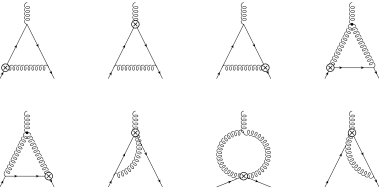
Fig. 1: Self mixing of operators $\bar{O}^{+}_{1\dots 8}$.

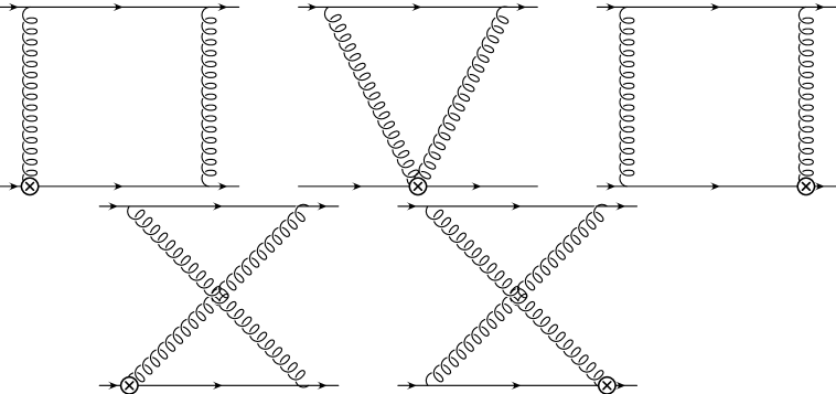
Fig. 2: Mixing of operators $\bar{O}^{+}_{1\dots 8}$ with $\bar{O}^{+}_{\left(11,\,n\right)},\bar{O}^{+}_{\left(12,\,n\right)}$.

We list in Fig. (1) and in Fig. (2) the general structure of the graphs needed to renormalize off-shell the operators $\bar{O}^{+}_{1,\dots 8}$: note that the graphs in Fig. (2) are proportional to $\alpha_{s}^{2}$, but as pointed by Misiak [19] they are required even at leading order since they give rise to the mixing of the operator $\bar{O}^{7}$ with the operators $\bar{O}^{+}_{\left(11,\,n\right),\,\left(12,\,n\right)}$ in consequence of the motion equations.

The computation of the Feynman graphs in Fig. (1) results in the $\left\{1\dots 8\right\}\times\left\{1\dots 8\right\}$ sector of the one-loop anomalous dimension matrix $\hat{\gamma}^{(1)}$,

$$\frac{\alpha_{s}}{4\pi}\>\bordermatrix{&1&2&3&4&5&6&7&8\cr 1&{\scriptstyle-2\,C_{F}\xi}&0&0&{\scriptstyle 6\,C_{F}}&0&0&0&0\cr 2&0&0&0&0&{\scriptstyle 8\,C_{F}}&0&0&0\cr 3&0&0&0&0&0&0&0&0\cr 4&0&0&0&{\scriptstyle 6\,C_{F}-2\,C_{F}\xi}&0&0&0&0\cr 5&0&0&0&0&{\scriptstyle 8\,C_{F}}&0&0&0\cr{\scriptstyle 6}&{\scriptstyle-12\,C_{F}}&{\scriptstyle 4\,C_{F}}&0&0&{\scriptstyle 4\,C_{F}}&{\scriptstyle 4\,C_{F}}&0&{\scriptstyle 4}{\scriptstyle(3\,C_{F}-C_{A})}\cr{\scriptstyle 7}&{\scriptstyle 2\,C_{F}}&0&{\scriptstyle\frac{8\,C_{F}}{3}}&0&0&0&{\scriptstyle\frac{8}{3}\,C_{F}+3\,C_{A}}&0\cr{\scriptstyle 8}&0&0&0&{\scriptstyle-12\,C_{F}}&{\scriptstyle 8\,C_{F}}&0&0&{\scriptstyle 4(4\,C_{F}-C_{A})}}\ ,$$ (42)

while the graphs in Fig. (2) connect the operator $\bar{O}^{+}_{7}$ to four fermion operators, resulting in

$$\left(\frac{\alpha_{s}}{4\pi}\right)^{2}\>\bordermatrix{&(11,1)&(11,3)&(12,1)&(12,3)\cr 7&\frac{-5+5\,C_{A}^{2}-10\,C_{A}\,C_{F}}{2}&\frac{9\,C_{A}^{2}-30\,C_{A}\,C_{F}+24\,C_{F}^{2}}{2}&0&\frac{24\,C_{F}-9\,C_{A}}{2}}\ .$$ (43)

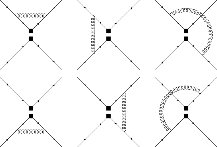
Fig. 3: Self mixing of $4$-fermion operators.

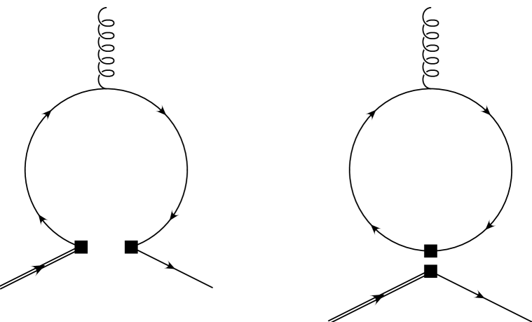
Fig. 4: Mixing of $4$-fermion operators with $\bar{O}^{+}_{1\dots 8}$ operators.

The renormalization of four fermion operators, off-shell, results from the graphs in Fig. (3) and in Fig. (4).

The self mixing of four fermion operators at one-loop, in Fig. (3), connects Dirac structures with $\mathchar 1\relax n={+2,\,0,\,-2}$

$$\frac{\alpha_{s}}{4\pi}\>\bordermatrix{&(9,n-2)&(9,n)&(9,n+2)\cr(9,n)&{{\left(6-n\right)\,\left(n-5\right)}\over{C_{A}}}&{\scriptstyle 2\,C_{F}\,\left(\left(1-n\right)\,\left(n-3\right)-\xi\right)}&{{-\left(\left(1+n\right)\,\left(2+n\right)\right)}\over{C_{A}}}\cr(10,n)&{{\left(n-6\right)\,\left(n-5\right)}\over 2}&{\scriptstyle 3\,\left(-2+4\,n-{n^{2}}\right)}&{{\left(1+n\right)\,\left(2+n\right)}\over 2}\cr}\ ,$$ (44)

$$\frac{\alpha_{s}}{4\pi}\>\bordermatrix{&(10,n-2)&(10,n)&(10,n+2)\cr(9,n)&{\scriptstyle\left(n-6\right)\,\left(n-5\right)}&0&{\scriptstyle\left(1+n\right)\,\left(2+n\right)}\cr(10,n)&{{\left(4\,C_{F}-\,C_{A}\right)\,\left(n-6\right)\,\left(n-5\right)}\over 2}&{\scriptstyle\left(3\,C_{A}-4\,C_{F}\right)\,\left(2-4\,n+{n^{2}}\right)-4\,C_{F}\,\left(1+\xi\right)}&{{\left(4\,C_{F}-\,C_{A}\right)\,\left(1+n\right)\,\left(2+n\right)}\over 2}\cr}\ .$$ (45)

The same mixings occur in the $\bar{O}^{+}_{(11,n),(12,n)}$ sector.

The penguin graphs in Fig. (4) give rise to the mixing of the 4-fermion operators with $\bar{O}^{+}_{3,\,7}$ at the $\alpha_{s}^{0}$ order

$$\bordermatrix{&3&7\cr(9,n)&-\frac{2\left(n-2\right)}{3n!}\left(-1\right)^{n}c_{n}(0)&\frac{(n-2)}{3n!}(-1)^{n}c_{n}(0)\cr(10,n)&-C_{A}\frac{2\left(n-2\right)}{3n!}(-1)^{n}c_{n}(0)&0\cr(11,n)&C_{A}\frac{8}{3}\bar{n}_{f}\delta_{n,1}+\frac{2\left(n-2\right)}{3n!}(-1)^{n}c_{n}(0)&\frac{2\left(n-2\right)}{3n!}(-1)^{n}c_{n}(0)\cr(12,n)&\frac{8}{3}\bar{n}_{f}\delta_{n,1}+C_{A}\frac{2\left(n-2\right)}{3n!}(-1)^{n}c_{n}(0)&\frac{8}{3}n_{f}\delta_{n,1}\cr}\ .$$ (46)

The meaning of the symbol $c_{n}$ is explained in App. B together with the other definitions and useful formulas. We use the symbols $n_{f}=u+d,\,\bar{n}_{f}=d-2\,u$, with $u$ and $d$ being the number of up and down quark species active.

It is to be noted that at leading order only the $n=\{1,\,3,\,5\}$ values are needed, because the effective hamiltonian starts with $n=\{1,\,3\}$ and at one loop only the $n=5$ evanescent arises. We find convenient to give also the results restricted to this set of $n$ values

$$\frac{\alpha_{s}}{4\pi}\>(\bordermatrix{&(9,1)&(9,3)&(9,5)&(10,1)&(10,3)&(10,5)\cr(9,1)&0&-\frac{6}{C_{A}}&0&0&6&0\cr(9,3)&-\frac{6}{C_{A}}&0&-\frac{20}{C_{A}}&6&0&20\cr(10,1)&3&3&0&-\frac{3}{C_{A}}-6\,C_{F}&-\frac{3}{C_{A}}+6\,C_{F}&0\cr(10,3)&3&3&10&-\frac{3}{C_{A}}+6\,C_{F}&-\frac{3}{C_{A}}-6\,C_{F}&20\,C_{F}-\frac{10}{C_{A}}\cr}\ ,$$ (47)

$$\bordermatrix{&3&7\cr(9,\,1)&-\frac{8}{3}&\frac{4}{3}\cr(9,\,3)&-\frac{8}{3}&\frac{4}{3}\cr(10,\,1)&-\frac{8\,C_{A}}{3}&0\cr(10,\,3)&-\frac{8\,C_{A}}{3}&0\cr(11,\,1)&\frac{8}{3}\left(1+C_{A}\,\bar{n}_{f}\right)&\frac{8}{3}\cr(11,\,3)&\frac{8}{3}&\frac{8}{3}\cr(12,\,1)&\frac{8}{3}\left(C_{A}+\,\bar{n}_{f}\right)&\frac{8}{3}n_{f}\cr(12,\,3)&\frac{8}{3}\,C_{A}&0}\ .$$ (48)

It is well known that renormalized operators proportional to motion equations mix only between themselves and that their anomalous dimension matrix is not gauge independent. In fact, we can observe that operator $N\left[{\bar{O}^{+}_{1}}\right]$, proportional to the $s$ motion equation, mixes only with itself and operator $N\left[{\bar{O}^{s}_{4}}\right]$: this one mixes with itself only, and both operators have anomalous dimension matrix depending on $\xi$ [30]. The difference $N\left[{\bar{O}^{+}_{2}-\bar{O}^{+}_{5}}\right]$ is proportional to a combination of the $s$ and $b$ motion equations and does not evolve at one-loop. Analogously the operator $N\left[{\bar{O}^{+}_{6}-\bar{O}^{+}_{8}}\right]$ mixes with itself and with $N\left[{\bar{O}^{+}_{1}}\right],\,N\left[{\bar{O}^{+}_{2}-\bar{O}^{+}_{5}}\right],\,N\left[{\bar{O}^{+}_{4}}\right]$. Finally the combination

$$N\left[{\bar{O}^{+}_{7}+\frac{\alpha_{s}}{4\pi}\left(\frac{1}{2\,C_{A}}\bar{O}^{+}_{(11,\,1)}-\frac{1}{2}\bar{O}^{+}_{(12,\,1)}\right)}\right]$$

is proportional to the equation of motion of the gluon. It is worth noting that the elimination of the operator $N\left[{\bar{O}^{+}_{7}}\right]$ in favor of the four fermion operators introduces a factor $\frac{1}{\alpha_{s}}$ which combines with the $\alpha_{s}^{2}$ in Eq. (43) to give a result relevant for the leading order computation [19].

3.3 Two loop results

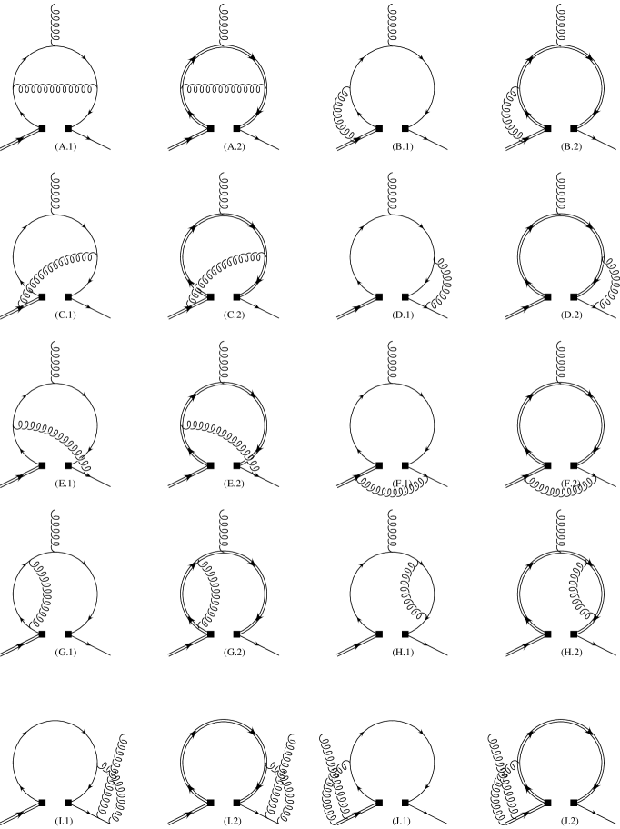
Fig. 5: “Open” graphs contributing to the renormalization of $\bar{O}^{+}_{\left(9-12,\,n\right)}$.

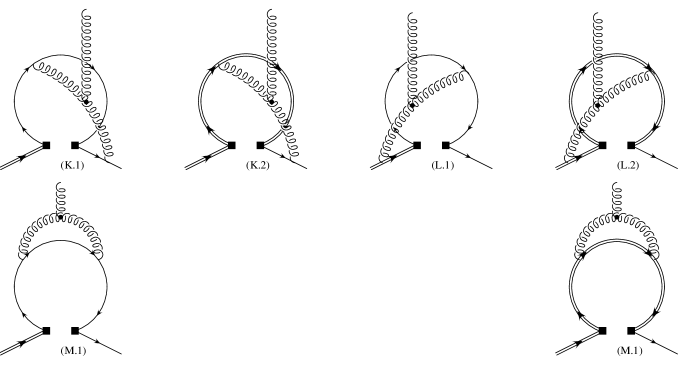
Fig. 6: “Open” graphs for the renormalization of $\bar{O}^{+}_{\left(9-12,\,n\right)}$. Non abelian couplings.

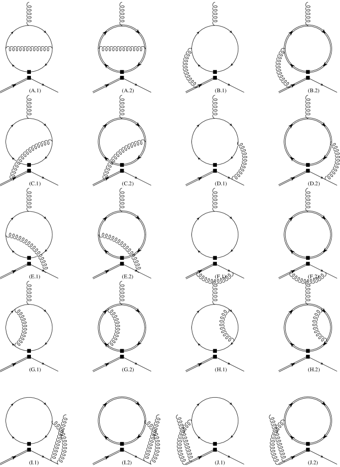
Fig. 7: ‘Closed” graphs contributing to the renormalization of $\bar{O}^{+}_{\left(11-12,\,n\right)}$.

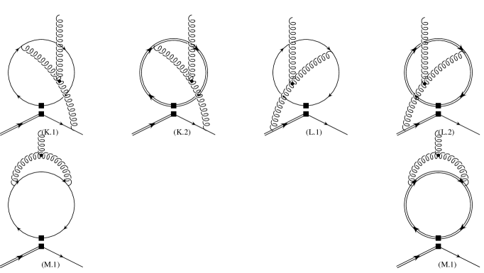
Fig. 8: “Closed” graphs for the renormalization of $\bar{O}^{+}_{\left(11-12,\,n\right)}$. Non abelian couplings.

The two-loop mixing of the four fermion operators with operators $\bar{O}^{+}_{1,\dots 8}$ can be obtained from the computation of the Feynman diagrams in Figs. (5, 6) and in Figs. (7, 8): the “closed” loop graphs are relevant only for the renormalization of operators $\bar{O}^{+}_{\left(\left(11-12\right),\,n\right)}$.

The massive $b$ quark is represented by the heavy-faced lines. The $b$ propagator is expanded in series of $m_{b}$ up to the first order and the resulting massless graphs are regularized in the infrared region by the flow of the external momenta: the diagrams have to be evaluated with zero and one mass insertions. The loop integrals have been computed with the help of the algorithms developed by Chetyrkin et al. [31], implemented in the Mathematica [32] symbolic manipulation language.

Table 1: Two loop ADM entries for $\bar{O}^{+}_{\left(9,\,n\right)},\,\bar{O}^{+}_{\left(10,\,n\right)}$, resulting from the mixing with $\bar{O}^{+}_{1},\,\bar{O}^{+}_{8}$

$\gamma$ entry
${(9,n),1}$	$\left(-1\right)^{n}\frac{C_{F}}{3n!}\left(\left(1-n\right)c_{n}(0)+\left(2-n\right)c_{n}(1)\right)$
${(9,n),2}$	$\frac{2\,C_{F}}{n!}\left[-f_{n,3}\left(0\right)+\left(-1\right)^{n}\frac{\left(2-n\right)}{9}c_{n}\left(0\right)\right]$
${(9,n),3}$	$\frac{4\,C_{F}}{n!}\left[-f_{n,3}(0)+\frac{n(n-1)(-1)^{n}}{18}\left(1908-1124n+213n^{2}-13n^{3}\right)c_{n-2}(0)\right.$
	$\left.\qquad+\frac{(-1)^{n}}{54}\left(160-290n+177n^{2}-33n^{3}\right)c_{n}(0)+\frac{2(n-2)(-1)^{n}}{9}\left(4-12n+3n^{2}\right)c_{n}(1)\right]$
${(9,n),4}$	$\frac{C_{F}\,\left(2-n\right)\left(-1\right)^{n}}{2n!}c_{n}(0)$
${(9,n),5}$	$\frac{2\,C_{F}\,\left(n-2\right)}{3n!}\left(2n^{2}-8n+3\right)\left(-1\right)^{n}c_{n}(0)$
${(9,n),6}$	$\frac{4\,C_{F}-C_{A}}{4n!}f_{n,3}(0)+\left(-1\right)^{n}\frac{\left(8\,C_{F}-9\,C_{A}\right)\left(2-n\right)}{36n!}c_{n}(0)$
${(9,n),7}$	${{\left(4\,C_{F}-C_{A}\right)\,f_{n,3}(0)}\over{2n!}}+{{{{\left(-1\right)}^{n}}\,\left(C_{A}-2\,C_{F}\right)\,n\,\left(n-1\right)}\over{18n!}}\,\left(1908-1124\,n+213\,{n^{2}}-13\,{n^{3}}\right)\,c_{n-2}(0)$
	$+{{\left(-1\right)^{n}}\over{108n!}}\,\left(3\,C_{A}\,\left(4-n\right)\,\left(3-46\,n+24\,{n^{2}}\right)-4\,C_{F}\,\left(58-230\,n+177\,{n^{2}}-33\,{n^{3}}\right)\right)\,c_{n}(0)$
	$+{{\left(-1\right)^{n}}\over{18n!}}\,\left(n-2\right)\,\left(4\,C_{F}\,\left(-11+24\,n-6\,{n^{2}}\right)+3\,C_{A}\,\left(-3-8\,n+2\,{n^{2}}\right)\right)\,c_{n}(1)$
${(9,n),8}$	${{{{\left(-1\right)}^{n}}\,\left(n-2\right)}\over{24n!}}\,\left(8\,C_{F}\,\left(-3+8\,n-2\,{n^{2}}\right)+C_{A}\,\left(1-16\,n+4\,{n^{2}}\right)\right)\,c_{n}(0)$
${(10,n),1\,(2)}$	0
${(10,n),3}$	$\frac{C_{A}\,C_{F}\left(-1\right)^{n}}{9n!}\left[n\,\left(n-1\right)\,\left(1908-1124\,n+213\,{n^{2}}-13\,{n^{3}}\right)\,c_{n-2}(0)\right.$
	$\left.\qquad+\left(108-148\,n+83\,{n^{2}}-13\,{n^{3}}\right)\,c_{n}(0)\right]$
${(10,n),4\,(5)}$	$0$
${(10,n),6}$	$\frac{1}{2n!}f_{n,3}(0)$
${(10,n),7}$	$\frac{1}{n!}f_{n,3}(0)+{{{{\left(-1\right)}^{n}}\,n\,\left(n-1\right)}\over{36n!}}\,\left(-1908+1124\,n-213\,{n^{2}}+13\,{n^{3}}\right)\,c_{n-2}(0)$
	$+{{\left(-1\right)^{n}}\over{36n!}}\,\left(24+32\,n-35\,{n^{2}}+9\,{n^{3}}\right)\,c_{n}(0)+{{{{\left(-1\right)}^{n}}\,\left(n-2\right)}\over{3n!}}\,\left(-3+8\,n-2\,{n^{2}}\right)\,c_{n}(1)$
${(10,n),8}$	${{{{\left(-1\right)}^{n}}\,\left(n-2\right)}\over{6n!}}\,\left(-3+8\,n-2\,{n^{2}}\right)\,c_{n}(0)$

Table 2: Two loop ADM entries for $\bar{O}^{+}_{\left(11,\,n\right)}$, resulting from the mixing with $\bar{O}^{+}_{1},\,\bar{O}^{+}_{8}$

$\gamma$ entry
${(11,n),1}$	$\frac{2\,C_{F}\,\left(-1\right)^{n}}{3\,n!}\left[\left(1-n\right)c_{n}(0)+\left(2-n\right)c_{n}(1)\right]$
${(11,n),2}$	$\frac{2\,C_{F}}{n!}\left[f_{n,\,3}(0)+\frac{2}{9}\left(2-n\right)\left(-1\right)^{n}c_{n}(0)\right]$
${(11,n),3}$	$\frac{C_{F}}{n!}\left[8\,C_{A}\,\bar{n}_{f}\delta_{n,\,1}+4\,f_{n,\,3}(0)\right.$
	$\qquad+\frac{2}{9}\,\left(-1\right)^{n}\,\left(n-1\right)\,n\,\left(-1908+1124\,n-213\,{n^{2}}+13\,{n^{3}}\right)\,c_{n-1}(0)$
	$\qquad+\frac{2}{27}\,\left(-1\right)^{n}\,\left(-58+230\,n-177\,{n^{2}}+33\,{n^{3}}\right)\,c_{n}(0)$
	$\qquad\left.+\frac{4}{9}\,(-1)^{n}\,\left(n-2\right)\,\left(-11+24\,n-6\,{n^{2}}\right)\,c_{n}(1)\right]$
${(11,n),4}$	$\frac{C_{F}}{n!}\left[\frac{1}{3}{\left(39-68\,n+20\,{n^{2}}+3\,\left(2-n\right)\left(-1\right)^{n}\right)\,c_{n}(0)}+2\,\left(n-3\right)\,\left(n-1\right)\,c_{n}(1)\right]$
${(11,n),5}$	$\frac{C_{F}}{3n!}\left[2\,\left(n-6\right)\,{{\left(n-5\right)}^{2}}\,\left(n-3\right)\,\left(n-1\right)\,n\,c_{n-2}(1)\right.$
	$\qquad-\frac{1}{3}{\left(45+100\,n-170\,{n^{2}}+56\,{n^{3}}-4\,{n^{4}}+2\,\left(n-2\right)\,\left(2\,n^{2}-8\,n+3\right)\left(-1\right)^{n}\right)\,c_{n}(0)}$
	$\left.\qquad+2\,\left(n-3\right)\,\left(n-1\right)\,\left(-5+3\,n-{n^{2}}\right)\,c_{n}(1)\right]$
${(11,n),6}$	$\frac{1}{n!}\left[12\,n_{f}\delta_{n,3}+\frac{1}{2}\left(4\,C_{F}-C_{A}\right)f_{n,3}(0)\right.$
	$\qquad\left.+\frac{\left(-1\right)^{n}}{18}\left(9\,C_{A}-8\,C_{F}\right)\left(n-2\right)c_{n}(0)\right]$
${(11,n),7}$	$\frac{1}{n!}\left[88\,n_{f}\delta_{n,3}+\left(4\,C_{F}-C_{A}\right)f_{n,3}(0)\right.$
	$\qquad+\frac{1}{9}\left(-1\right)^{n}\,\left(2\,C_{F}-C_{A}\right)\,\left(n-1\right)\,n\,\left(-1908+1124\,n-213\,{n^{2}}+13\,{n^{3}}\right)\,c_{n-2}(0)$
	$\qquad+\frac{1}{54}\left(-1\right)^{n}\left(3\,C_{A}\,\left(n-4\right)\,\left(-3+46\,n-24\,{n^{2}}\right)\right.+$
	$\qquad+\left.4\,\,C_{F}\,\left(-58+230\,n-177\,{n^{2}}+33\,{n^{3}}\right)\right)\,c_{n}(0)$
	$\left.\qquad+\frac{1}{9}\left(-1\right)^{n}\left(2-n\right)\,\left(3\,C_{A}\,\left(3+8\,n-2\,{n^{2}}\right)+4\,C_{F}\,\left(11-24\,n+6\,{n^{2}}\right)\right)\,c_{n}(1)\right]$
${(11,n),8}$	$\frac{1}{n!}\left[\frac{1}{3}{\left(-C_{A}+2\,C_{F}\right)\,\left(n-6\right)\,{{\left(n-5\right)}^{2}}\,\left(n-3\right)\,\left(n-1\right)\,n\,c_{n-2}(1)}\right.$
	$\qquad+\frac{1}{18}\left(C_{A}\,\left(99+24\,n-125\,{n^{2}}+40\,{n^{3}}-2\,{n^{4}}\right)+\right.$
	$\qquad+\left.2\,C_{F}\,\left(-45-100\,n+170\,{n^{2}}-56\,{n^{3}}+4\,{n^{4}}\right)\right)\,c_{n}(0)$
	$\qquad+\frac{1}{3}{\left(n-3\right)\,\left(n-1\right)\,\left(C_{A}\,n+2\,C_{F}\,\left(-5+3\,n-{n^{2}}\right)\right)\,c_{n}(1)}+24\,n_{f}\,\delta_{n,3}$
	$\qquad\left.+\frac{1}{12}\left(-1\right)^{n}\left(n-2\right)\,\left(8\,C_{F}\,\left(-3+8\,n-2\,{n^{2}}\right)+C_{A}\,\left(1-16\,n+4\,{n^{2}}\right)\right)\,c_{n}(0)\right]$

Table 3: Two loop ADM entries for $\bar{O}^{+}_{\left(12,\,n\right)}$, resulting from the mixing with $\bar{O}^{+}_{1},\,\bar{O}^{+}_{8}$

$\gamma$ entry
${(12,n),1}$	$-\frac{4}{3}\,C_{F}n_{f}\delta_{n,1}$
${(12,n),2}$	$-\frac{16}{9}\,C_{F}n_{f}\delta_{n,1}+4\,C_{F}\bar{n}_{f}\delta_{n,3}$
${(12,n),3}$	$-\frac{8}{81}\,C_{F}\left(102n_{f}-81\bar{n}_{f}\right)\delta_{n,1}+\frac{88}{3}\,C_{F}\bar{n}_{f}\delta_{n,3}$
	$\qquad+\frac{C_{A}\,C_{F}\,\left(-1\right)^{n}}{9\,n!}\left[\left(n-1\right)\,n\,\left(-1908+1124\,n-213\,{n^{2}}+13\,{n^{3}}\right)\,c_{n-2}(0)\right.$
	$\qquad\qquad\left.+\left(-108+148\,n-83\,{n^{2}}+13\,{n^{3}}\right)\,c_{n}(0)\right]$
${(12,n),4}$	$-4\,C_{F}n_{f}\delta_{n,1}$
${(12,n),5}$	$\frac{C_{A}\,C_{F}}{3\,n!}\,\left[\left(n-6\right)\,{{\left(n-5\right)}^{2}}\,\left(n-3\right)\,\left(n-1\right)\,n\,c_{n-2}(1)\right.$
	$\qquad+\frac{1}{3}\left(45-80\,n+56\,{n^{2}}-12\,{n^{3}}\right)\,c_{n}(0)$
	$\left.\qquad+\left(n-3\right)\,\left(n-1\right)\,\left(-2-5\,n+{n^{2}}\right)\,c_{n}(1)\right]+8\,C_{F}\,\bar{n}_{f}\,\delta(n,3)$
${(12,n),6}$	$\frac{1}{n!}\,f_{n,3}(0)+\frac{2}{9}\,\left(9\,C_{A}-8\,C_{F}\right)\,n_{f}\,\delta_{n,1}+\left(4\,C_{F}-C_{A}\right)\,n_{f}\,\delta_{n,3}$
${(12,n),7}$	$\frac{28}{27}\left(9\,C_{A}-2\,C_{F}\right)n_{f}\delta_{n,1}+\frac{22}{3}\left(4\,C_{F}-C_{A}\right)n_{f}\delta_{n,3}+\frac{2}{n!}f_{n,3}(0)$
	$\frac{\left(-1\right)^{n}}{3n!}\left[\frac{1}{6}\left(n-1\right)\,n\,\left(-1908+1124\,n-213\,{n^{2}}+13\,{n^{3}}\right)\,c_{n-2}(0)\right.$
	$\qquad+\frac{1}{6}\left(24+32\,n-35\,{n^{2}}+9\,{n^{3}}\right)\,c_{n}(0)$
	$\qquad+2\,\left(2-n\right)\,\left(3-8\,n+2\,{n^{2}}\right)\,c_{n}(1)$
${(12,n),8}$	$\frac{-5\,C_{A}}{3}n_{f}\delta_{n,1}+2\,\left(4\,C_{F}-C_{A}\right)\,n_{f}\delta_{n,3}$
	$+\frac{1}{3\,n!}\left[\frac{1}{2}\left(n-6\right)\,{{\left(n-5\right)}^{2}}\,\left(n-3\right)\,\left(n-1\right)\,n\,c_{n-2}(1)\right.$
	$\quad+\frac{1}{3}\left(73\,{n^{2}}-18-62\,n-22\,{n^{3}}+2\,{n^{4}}\left(-1\right)^{n}\,\left(18-57\,n+36\,n^{2}-6\,n^{3}\right)\right)\,c_{n}(0)$
	$\left.\quad+\frac{1}{2}\left(n-3\right)\,\left(n-1\right)\,\left(-4+11\,n-3\,{n^{2}}\right)\,c_{n}(1)\right]$

As in the case of the one loop computation, the results can be given for arbitrary $n$ and are listed in Tabb. (1, 2, 3). We refer to App. B for symbols and definitions; let us just note that the symbol $f_{n\,j}$ results from traces involving elements of the $\{\gamma^{\left({n}\right)}\}$ basis.

We stress that having the results for arbitrary $n$ will be useful for the NLO computation.

3.4 Reduction of evanescent operators

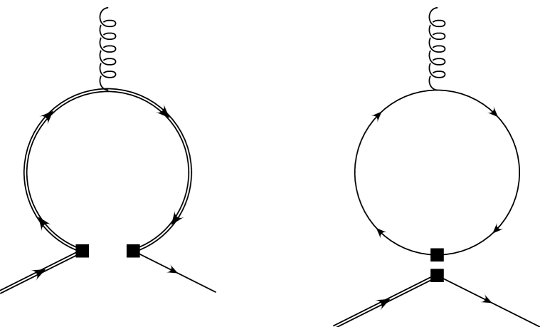
Fig. 9: Diagrams relevant at LO for the reduction of evanescent operators.

Before giving the results for $n=1,\,3$, that are needed in this leading logarithmic computation, we perform the reduction of the evanescent operators with $n=5$. The scheme we follow is detailed in App. A.1, and requires the computation of the graphs in Fig. (9), which allows to express the insertion of the evanescent operators in the Green functions in terms of the insertion of relevant operators, with coefficients addressed by the matrix $\hat{r}$

$$\hat{r}=\bordermatrix{&3&5&7&8\cr(9,5)&\frac{2}{5}&0&-\frac{1}{5}&0\cr(10,5)&\frac{2}{5}\,C_{A}&0&0&0\cr(11,5)&-\frac{2}{5}&\frac{8}{15}&-\frac{2}{5}&\frac{8}{15}\cr(12,5)&-\frac{2}{5}\,C_{A}&\frac{8}{15}\,C_{A}&0&0\cr}.$$ (49)

For the present computation only columns $5,\,8$ are relevant, while the columns $3,\,7$ contribute through equations of motion to four fermion operators,

$$\hat{r}_{\mathrm{on-shell}}=\frac{\alpha_{s}}{4\pi}\bordermatrix{&(11,1)&(12,1)\cr(9,5)&\frac{1}{10\,C_{A}}&-\frac{1}{10}\cr(10,5)&0&0\cr(11,5)&\frac{1}{5\,C_{A}}&-\frac{1}{5}\cr(12,5)&0&0\cr}\ ,$$ (50)

and are relevant only for the NLO computation.

By combining the reduction coefficients in Eq. (49), the one loop anomalous dimension matrix in Eq. (47) and the results of the two loop computation listed in Tabb. (1, 2, 3), we are able to give the anomalous dimension matrix relevant at leading order, where a factor $\frac{\alpha_{s}}{4\,\pi}$ is understood.

$$\bordermatrix{&1&2&3&4\cr(9,\,1)&{{2\,C_{F}}\over 3}&{{-44\,C_{F}}\over 9}&{{-88\,C_{F}}\over{27}}&-2\,C_{F}\cr(9,\,3)&{{2\,C_{F}}\over 9}&{{-44\,C_{F}}\over 9}&8\,C_{A}-{{1688\,C_{F}}\over{27}}&-2\,C_{F}\cr(10,\,1)&0&0&{{-40\,C_{A}\,C_{F}}\over 3}&0\cr(10,\,3)&0&0&{{4\,C_{A}\,\left(3-14\,C_{F}\right)}\over 3}&0\cr(11,\,1)&{{4\,C_{F}}\over 3}&{{20\,C_{F}}\over 9}&{{-176\,C_{F}}\over{27}}+{{8\,C_{A}\,C_{F}\,\bar{n}_{f}}\over 3}&-16\,C_{F}\cr(11,\,3)&{{4\,C_{F}}\over 9}&{{20\,C_{F}}\over 9}&{{944\,C_{F}}\over{27}}&-24\,C_{F}\cr(12,\,1)&{{4\,C_{F}\,\left(2\,\bar{n}_{f}-3\,n_{f}\right)}\over 9}&{{16\,C_{F}\,\left(2\,\bar{n}_{f}-3\,n_{f}\right)}\over{27}}&{{40\,C_{A}\,C_{F}}\over 3}+{{8\,C_{F}\,\left(95\,\bar{n}_{f}-102\,n_{f}\right)}\over{81}}&{{4\,C_{F}\,\left(2\,\bar{n}_{f}-3\,n_{f}\right)}\over 3}\cr(12,\,3)&0&{{4\,C_{F}\,\bar{n}_{f}}\over 3}&{{32\,C_{A}\,C_{F}}\over 3}+{{88\,C_{F}\,\bar{n}_{f}}\over 9}&0\cr}$$ (51)

$$\bordermatrix{&5&6\cr(9,\,1)&-8\,C_{F}&{{C_{A}}\over 2}+{{10\,C_{F}}\over 9}\cr(9,\,3)&-8\,C_{F}&{{C_{A}}\over 2}+{{10\,C_{F}}\over 9}\cr(10,\,1)&0&1\cr(10,\,3)&0&1\cr(11,\,1)&-4\,C_{F}&C_{A}+{{20\,C_{F}}\over 9}\cr(11,\,3)&{{-32}\over{3\,C_{A}}}+{{32\,C_{A}}\over 3}+{{28\,C_{F}}\over 3}&C_{A}+{{20\,C_{F}}\over 9}+2\left(n_{f}-\frac{2}{3}\bar{n}_{f}\right)\cr(12,\,1)&4\,C_{A}\,C_{F}&2+{{\left(16\,C_{F}-18\,C_{A}\right)\,\left(2\,\bar{n}_{f}-3\,n_{f}\right)}\over{27}}\cr(12,\,3)&{{52\,C_{A}\,C_{F}}\over 3}+{{8\,C_{F}\,\bar{n}_{f}}\over 3}&2+{{\left(4\,C_{F}-C_{A}\right)\,\left(3\,n_{f}-2\,\bar{n}_{f}\right)}\over 3}}$$ (52)

$$\bordermatrix{&7&8\cr(9,\,1)&{{25\,C_{A}}\over 3}-{{88\,C_{F}}\over{27}}&{{-11\,C_{A}}\over 6}+4\,C_{F}\cr(9,\,3)&{{-5\,C_{A}}\over 3}+{{688\,C_{F}}\over{27}}&{{-11\,C_{A}}\over 6}+4\,C_{F}\cr(10,\,1)&-{{10}\over 3}&2\cr(10,\,3)&10&2\cr(11,\,1)&{{50\,C_{A}}\over 3}-{{176\,C_{F}}\over{27}}&{{13\,C_{A}}\over 3}-4\,C_{F}\cr(11,\,3)&{{944\,C_{F}+126\,C_{A}}\over 27}+{{44}\over 3}\,\left(n_{f}-\frac{2}{3}\bar{n}_{f}\right)&{{92\,C_{F}-19\,C_{A}}\over 3}+4\left(n_{f}-\frac{2}{3}\bar{n}_{f}\right)\cr(12,\,1)&-{{20}\over 3}+{{\left(56\,C_{F}-252\,C_{A}\right)\,\left(2\,\bar{n}_{f}-3\,n_{f}\right)}\over{81}}&-8+{{5\,C_{A}\,\left(2\,\bar{n}_{f}-3\,n_{f}\right)}\over 9}\cr(12,\,3)&16+{{22\,\left(4\,C_{F}-C_{A}\right)\,\left(3\,n_{f}-2\,\bar{n}_{f}\right)}\over 9}&{{2\,\left(4\,C_{F}-C_{A}\right)\,\left(3\,n_{f}-2\,\bar{n}_{f}\right)}\over 3}}\ .$$ (53)

3.5 On-shell results

By applying the motion equations, it is now possible to give the results in the following on-shell basis which closely corresponds to the symmetrization of the one used by Ciuchini et al. [7, 33],

$$Q^{+}_{1} = \bar{Q}_{1}^{+}-E_{1}^{+}=\bar{O}^{+}_{(9,\,1)}+\bar{O}^{+}_{(9,\,3)}-E_{1}^{+}$$

$$Q^{+}_{2} = \bar{Q}_{2}^{+}-E_{2}^{+}=\bar{O}^{+}_{(10,\,1)}+\bar{O}^{+}_{(10,\,3)}-E_{2}^{+}$$

$$Q^{+}_{3/5} = \bar{Q}_{3/5}^{+}-E_{3/5}^{+}=\bar{O}^{+}_{(11,\,1)}\pm\bar{O}^{+}_{(11,\,3)}-E_{3/5}^{+}$$

$$Q^{+}_{4/6} = \bar{Q}_{4/6}^{+}-E_{4/6}^{+}=\bar{O}^{+}_{(12,\,1)}\pm\bar{O}^{+}_{(12,\,3)}-E_{4/6}^{+}$$

$$Q^{+}_{7} = \bar{Q}_{7}^{+}=\bar{O}^{+}_{5}$$

$$Q^{+}_{8} = \bar{Q}_{8}^{+}=\bar{O}^{+}_{8}$$

$$Q^{+}_{9} = \bar{Q}_{9}^{+}-E_{9}^{+}=\bar{O}^{+}_{(9,\,1)}-\bar{O}^{+}_{(9,\,3)}-E_{9}^{+}$$

$$Q^{+}_{10} = \bar{Q}_{10}^{+}-E_{10}^{+}=\bar{O}^{+}_{(10,\,1)}-\bar{O}^{+}_{(10,\,3)}-E_{10}^{+}\ .$$ (54)

The last two operators have been introduced to have an invertible relation between the bases $\bar{O}^{+}_{i}$ and $Q^{+}_{i}$; as expected they decouple from the others in the RG evolution. The presence of the evanescent operators takes into account the difference in the $d$-dimensional extensions, as explained in section 2.1. In the basis $\bar{Q}_{i}^{+}$ we give the final results for the AD matrix in the following block form:

$$\hat{\gamma}=\frac{\alpha_{s}}{4\pi}\>\left(\begin{array}[]{cc}\hat{\gamma}_{ff}&\hat{\gamma}_{fm}\cr\hat{0}&\hat{\gamma}_{mm}\end{array}\right)\ .$$ (55)

The matrices $\hat{\gamma}_{ff},\,\hat{\gamma}_{mm}$ result from the one loop computation and are scheme independent; they guide the RG evolution respectively in the four fermion and in the magnetic momentum sectors,

$$\hat{\gamma}_{ff} = \bordermatrix{&1&2&3&4&5&6\cr 1&-\frac{6}{C_{A}}&6&0&0&0&0\cr 2&6&-\frac{6}{C_{A}}&-\frac{2}{3\,C_{A}}&\frac{2}{3}&-\frac{2}{3\,C_{A}}&\frac{2}{3}\cr 3&0&0&-\frac{22}{3\,C_{A}}&\frac{22}{3}&-\frac{4}{3\,C_{A}}&\frac{4}{3}\cr 4&0&0&\frac{2\left(9\,C_{A}-n_{f}\right)}{3\,C_{A}}&-\frac{2\left(9-n_{f}\,C_{A}\right)}{3\,C_{A}}&-\frac{2\,n_{f}}{3\,C_{A}}&\frac{2\,n_{f}}{3}\cr 5&0&0&0&0&\frac{6}{C_{A}}&-6\cr 6&0&0&-\frac{2\,n_{f}}{3\,C_{A}}&\frac{2\,n_{f}}{3}&-\frac{2\,n_{f}}{3\,C_{A}}&\frac{2\left(n_{f}-18\,C_{F}\right)}{3}}\ ,$$

$$\hat{\gamma}_{mm} = \bordermatrix{&7&8\cr 7&8\,C_{F}&0\cr 8&8\,C_{F}&16\,C_{F}-4\,C_{A}}\ .$$ (56)

The matrix $\gamma_{fm}$ connecting the four fermion and the magnetic momentum sectors results from the two-loop computation and it is scheme dependent, even at leading order, as pointed out by Ciuchini et al. [7, 33]

$$\hat{\gamma}_{fm}=\bordermatrix{&7&8\cr 1&0&6\cr 2&-\frac{232\,C_{F}}{9}&-\frac{8\,C_{A}}{3}+\frac{92\,C_{F}}{9}\cr 3&\frac{280\,C_{F}}{9}&\frac{280\,C_{F}}{9}+6\,n_{f}\cr 4&\frac{64\,C_{A}\,C_{F}}{3}+\frac{4\,C_{F}}{9}\left(27\,\bar{n}_{f}-4\,n_{f}\right)&-4-\frac{8\,C_{A}}{3}\,n_{f}+\frac{92\,C_{F}}{9}\,n_{f}\cr 5&-\frac{104\,C_{F}}{3}&\frac{32\,C_{A}}{3}-\frac{104\,C_{F}}{3}-6\,n_{f}\cr 6&-\frac{40\,C_{A}\,C_{F}}{3}-\frac{4\,C_{F}}{9}\left(4\,n_{f}+27\,\bar{n}_{f}\right)&-8+\frac{10\,C_{A}}{3}n_{f}-\frac{124\,C_{F}}{9}n_{f}}\ .$$ (57)

3.6 Matrix elements and scheme independence

The scheme dependence of the matrix $\hat{\gamma}_{fm}$ is compensated in the physical amplitude by the matrix elements of the four fermion operators.

The “even” contribution to the amplitude for the $b\rightarrow s\gamma$ decay has the form

$$<s\gamma|{\cal H}_{eff}^{+}|b>=\bar{C}^{s}_{7}\left<s\gamma\left|N\left[{Q^{+}_{7}}\right]\right|b\right>_{0}+\sum_{n=3}^{6}\bar{C}^{s}_{n}\left<s\gamma\left|N\left[{Q^{+}_{n}}\right]\right|b\right>_{1}$$ (58)

where the subscripts $0,\,1$ address the order in $\hbar$ of the matrix element, and an analogous formula holds for the $b\rightarrow sg$ amplitude .

The one loop matrix elements of the operators $Q^{+}_{3,\,4,\,5,\,6}$ result from Feynman diagrams analogous to the ones listed in Fig. (9) and with a mass insertion. If we define our scheme preserving the naive four dimensional Fierz simmetry they give a zero result. In fact in this case the “open” diagram in Fig. (9) with a mass insertion is proportional to the “closed” one, which is set to zero by the trace. The symmetry can be preserved by using the $HV$ scheme for $\gamma_{5}$ and maintaining the four dimensional definition for the current-current products [33].

In other regularization schemes this is no longer true and in general one obtains a local, finite contribution. This difference can be reinterpreted as a finite correction to the coefficient $C^{s}_{7}$ or alternatively, according to the discussion at the end of Sec. (2.1), to the operators. In our scheme the following relations hold

$${\left<s\gamma\left|\left(\begin{array}[]{c}\bar{O}^{+}_{11,n}\cr\bar{O}^{+}_{12,n}\cr\end{array}\right)\right|b\right>_{1}=}$$ (61)

$$\left({{\left(-36+64\,n-19\,{n^{2}}\right)}\over{36}}\frac{c_{n}(0)}{n!}+{{\left(1-n\right)\,\left(-3+n\right)}\over 6}\,\frac{c_{n}(1)}{n!}\right)\left(\begin{array}[]{c}1\cr C_{A}\end{array}\right)\left<s\gamma\left|\bar{O}^{+}_{5}\right|b\right>_{0}$$ (64)

$${\left<sg\left|\left(\begin{array}[]{c}\bar{O}^{+}_{11,n}\cr\bar{O}^{+}_{12,n}\cr\end{array}\right)\right|b\right>_{1}=}$$ (67)

$$\left({{\left(-36+64\,n-19\,{n^{2}}\right)}\over{36}}\frac{c_{n}(0)}{n!}+{{\left(1-n\right)\,\left(-3+n\right)}\over 6}\,\frac{c_{n}(1)}{n!}\right)\left(\begin{array}[]{c}1\cr 0\end{array}\right)\left<sg\left|\bar{O}^{+}_{8}\right|b\right>_{0}\ .$$ (70)

Using the definitions in Eq. (54) we can write

$$\left<s\,\gamma\left|\bar{Q}^{+}_{i}\right|b\right> = Z_{7i}\left<s\,\gamma\left|\bar{Q}^{+}_{7}\right|b\right>\qquad i=\{1\dots 6\}$$

$$\left<s\,g\left|\bar{Q}^{+}_{i}\right|b\right> = Z_{8i}\left<s\,g\left|\bar{Q}^{+}_{8}\right|b\right>\qquad i=\{1\dots 6\}$$ (71)

where following [7] we define the vectors

$$\vec{Z}_{7} = \left(0,0,\frac{8}{3},\frac{8\,C_{A}}{3},-\frac{2}{3},-\frac{2\,C_{A}}{3},0,0\right)$$

$$\vec{Z}_{8} = \left(0,0,\frac{8}{3},0,-\frac{2}{3}\ ,0,0,0\right)\ .$$ (72)

Following the steps outlined in Sec. 2 we perform the finite renormalizations needed to compare the results with the ones obtained in the HV scheme. We match the renormalization schemes by defining a non-minimal subtraction

$$N^{\prime}\left[{\bar{Q}^{+}_{i}}\right] = \left(\hat{1}+\delta\hat{F}\right)_{i\,j}N\left[{\bar{Q}^{+}_{j}}\right]$$

$$\delta\hat{F}_{i\,j} = \left\{\begin{array}[]{lr}-Z_{j\,i}&j=\left\{7,\,8\right\}\cr 0&j=\left\{1,\dots\,6\right\}\end{array}\right.$$ (75)

which sets to zero the matrix elements in Eq. (71), as they are in the HV scheme.

According to the formula in Eq. (A.14) the AD matrix is modified as follows

$$\hat{\gamma}^{\prime}=\left(\hat{1}+\delta\hat{F}\right)\hat{\gamma}\left(\hat{1}+\delta\hat{F}\right)^{-1}\ .$$ (76)

Using the results in Eq. (72), one easily obtains the AD matrix in the HV scheme

$$\hat{\gamma}^{\prime}_{mf}=\bordermatrix{&7&8\cr 1&0&6\cr 2&-\frac{208\,C_{F}}{9}&\frac{116\,C_{F}}{9}-4\,C_{A}\cr 3&\frac{232\,C_{F}}{9}&\frac{232\,C_{F}}{9}-8\,C_{A}+6n_{f}\cr 4&\frac{8\,C_{F}}{9}\,n_{f}+12\,C_{F}\,\bar{n}_{f}&12+\left(\frac{116\,C_{F}}{9}-4\,C_{A}\right)n_{f}\cr 5&-16\,C_{F}&4\,C_{A}-16\,C_{F}-6\,n_{f}\cr 6&\frac{8\,C_{F}}{9}\,n_{f}-12\,C_{F}\,\bar{n}_{f}&-8+\left(2\,C_{A}-\frac{100\,C_{F}}{9}\right)n_{f}}$$ (77)

which coincides with the result in [7].

Recall that in Eq. (75) we have imposed that the renormalized operators in the symmetrized scheme have the same matrix elements as in the HV scheme: moreover, at LO the coefficients at $\mu\simeq M_{W}$, relevant for the $b\rightarrow s\gamma$, are unaffected by the scheme redefinition, hence we conclude that the two schemes are completely equivalent. In other words the physical amplitude is now determined by the evolved coefficients (in the “symmetrized” scheme supplemented with the finite renormalization) and by the operators renormalized in the HV scheme.

At NLO it will be necessary a two loop matching of the schemes, but the three loop computations will be performed only in the symmetrized scheme.

4 Checks of the two loop computation

In this section we want to discuss the redundancy of the computation, which has been used in this work as a check of the computer codes and of the method itself; this can be of great help to reduce the complexity of a future NLO computation.

4.0.1 Fierz Identities

The generalized Fierz Identity [23, 25] listed in App. B, Eq. B.20, allow to relate “bare” graphs with a closed loop, listed in Figs. (5,6), with the ones with an open loop, listed in Figs. (7,8).

In other words, let $Closed\left(n\right)$ be the result of a graph with a closed loop, barring the sign coming from the fermionic loop and any color or flavor structure, and let $Open\left(n\right)$ be the corresponding graph with an open loop, having exactly the same “topology”: corresponding graphs in Figs. (5,6) and (7,8) are examples of such pairs and the index $n$ addresses the order of the $\left(\gamma^{\left({n}\right)}\otimes\gamma^{\left({n}\right)}\right)$ operator inserted.

Then the following relation holds:

$$Open\left(n\right)=\frac{1}{\mathrm{Tr}\left(1\right)}*\sum_{j=1}^{\infty}\frac{1}{j!}\left(-1\right)^{\frac{j\,(j-1)}{2}}f_{n\,j}Closed\left(j\right).$$ (78)

By expanding both members in powers of $\varepsilon$  and noting that on the right hand side only a finite number of terms can contribute, at a given perturbative order, one gets relations among the double and the single poles. Therefore the computation of one of the two sets of massless and massive graphs would be enough (as far as the “bare” part is concerned), provided one maintains $n$ arbitrary. Note that not only odd values of $n$ are needed and that is the reason why we have kept all values of $n$, despite the fact that only odd values of $n$ appear in the anomalous dimension matrices. This trick is not straightforwardly applicable when dealing with a counterterm graph if the four fermion vertex belongs to one of the divergent subgraphs considered. In fact in this case the subtraction recipe imposes the substitution of the subgraphs with the respective pole parts; this operation spoils the Fierz identity, since it is a “projection” on the physical $4$-dimensional space that does not commute with the transformation in Eq. (78).

4.0.2 Charge Conjugation

Let us recall the properties of the charge conjugation operator in euclidean notation

$$C^{-1}\gamma_{\mu}^{T}C = -\gamma_{\mu}\,$$

$$C^{T}=C^{\dagger} = -C=C^{-1}\,$$

$$CC^{\dagger}=C^{\dagger}C = -C^{2}=1\,$$ (79)

$$C^{-1}\gamma^{\left({n}\right)}C = \left(-1\right)^{n}\gamma^{\left({n}\right)}\,$$

$$C^{-1}\left(\gamma^{\left({n}\right)}\right)^{T}C = \left(-1\right)^{\frac{n\,\left(n+1\right)}{2}}\gamma^{\left({n}\right)}\ .$$

The last pair of relations is trivially derived by inserting $CC^{-1}$ factors in between $\gamma$ matrices and using

$$\left(\gamma^{\left({n}\right)}\right)^{T}=\left(-1\right)^{\frac{n\,\left(n-1\right)}{2}}\gamma^{\left({n}\right)}\ .$$ (80)

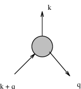
Fig. 10: Naming of external momenta in the two loop diagrams

We will take as reference Fig. (10) for the flow of momenta and Figs. (5, 6, 7, 8) for the naming of graphs.

Open loops

Sandwiching the graphs in Fig. (5) between $C^{-1}$ and $C$, it is easy to show that the following relations hold

$$C^{-1}A^{T}\left(k,\,q\right)C = -A\left(k,\,-k-q\right)$$

$$C^{-1}B^{T}\left(k,\,q\right)C = -D\left(k,\,-k-q\right)$$

$$C^{-1}C^{T}\left(k,\,q\right)C = -E\left(k,\,-k-q\right)$$

$$C^{-1}F^{T}\left(k,\,q\right)C = -F\left(k,\,-k-q\right)$$

$$C^{-1}G^{T}\left(k,\,q\right)C = -H\left(k,\,-k-q\right)$$

$$C^{-1}I^{T}\left(k,\,q\right)C = -J\left(k,\,-k-q\right)$$

$$C^{-1}K^{T}\left(k,\,q\right)C = -L\left(k,\,-k-q\right)$$

$$C^{-1}M^{T}\left(k,\,q\right)C = -M\left(k,\,-k-q\right)$$ (81)

Therefore most graphs are paired; for $A,\,F,\,M$ the relation is trivially satisfied. It is also worth remembering that the relations among graphs with the trilinear gluon vertex take into account its antisymmetry properties, once the same color factor is factorized for the three $K,\,L,\,M$ graphs.

Closed loops

In this case, see Figs. (7, 8), we have two fermionic lines, one traced and the other connected to the “in” and “out” states. Hence two sets of relations are possible.

By exploiting $C$ invariance on the external line, one gets the relations

$$C^{-1}B^{T}\left(k,\,q\right)C = \left(-1\right)^{\frac{n\,\left(n-1\right)}{2}}E\left(k,\,-k-q\right)$$

$$C^{-1}D^{T}\left(k,\,q\right)C = \left(-1\right)^{\frac{n\,\left(n-1\right)}{2}}C\left(k,\,-k-q\right)$$

$$C^{-1}F^{T}\left(k,\,q\right)C = \left(-1\right)^{\frac{n\,\left(n+1\right)}{2}}F\left(k,\,-k-q\right)$$

$$C^{-1}I^{T}\left(k,\,q\right)C = \left(-1\right)^{\frac{n\,\left(n+1\right)}{2}}J\left(k,\,-k-q\right)$$

$$C^{-1}K^{T}\left(k,\,q\right)C = -\left(-1\right)^{\frac{n\,\left(n-1\right)}{2}}L\left(k,\,-k-q\right)$$ (82)

while inserting a $CC^{-1}$ factor in the fermion loop, one is able to turn a clockwise loop in an anti-clockwise one, thus obtaining the relations

$$B\left(k,\,q\right) = \left(-1\right)^{\frac{n\,\left(n+1\right)}{2}}C\left(k,\,q\right)$$

$$D\left(k,\,q\right) = \left(-1\right)^{\frac{n\,\left(n+1\right)}{2}}E\left(k,\,q\right)$$

$$G\left(k,\,q\right) = \left(-1\right)^{\frac{n\,\left(n-1\right)}{2}}H\left(k,\,q\right)$$

$$M\left(k,\,q\right) = -\left(-1\right)^{\frac{n\,\left(n+1\right)}{2}}M\left(k,\,q\right)$$ (83)

By using the Fierz Identities and the relations coming from the charge conjugation, one reduces the computation of $26$ graphs to that of at most $10$.

4.0.3 Non local poles cancellation.

The total counterterm part of a two loop graphs exhibits a double pole with a coefficient twice the double pole in the “bare” graphs, thus ensuring the cancellation of non-local poles. This has been verified, together with the explicit cancellation of the logarithms, which is afurther test of the computer codes.

4.0.4 Gauge Invariance

We have verified that the gauge invariant basis off-shell, Eq. (40), is a complete basis; therefore all the results can be expressed in an explicit gauge invariant way, even off-shell, thanks to the background gauge-fixing.

The gauge invariance reflects itself in the fact that the Ward Identities for the vertex

$$k_{\mu}V^{b\rightarrow s\gamma}_{\mu}\left(k+q,\,q\right)\propto S_{s}\left(q\right)-S_{b}\left(k+q\right)$$ (84)

apply separately for different classes of graphs; therefore the groups

• {A, G, H}

• {B, C, J}

• {D, E, I}

• {F}

• {K, L, M}

can be individually checked.

4.0.5 Gauge Independence

All the graphs have been evaluated with an arbitrary background gauge fixing, depending on a parameter $\xi$. It is known that the resulting anomalous dimensions, on-shell, are independent from this gauge parameter: gauge dependence is possible only for operators proportional to the motion equations, which are zero on-shell, as we have seen in Sec. 3.2. The cancellation is effective among classes of graphs which are separately gauge independent: it is also worth noting that the cancellation holds separately for the two Casimir invariants, $C_{A}$ and $C_{F}$.

5 Conclusions

In this work we have detailed the computation of the leading logarithmic corrections to the $b\rightarrow s\gamma$ decay, presented in [5], which confirms the results of Ciuchini et al. [7, 8].

The application to this problem of the method introduced in [6] appears successful and the practical implementation provides relevant simplifications over the only other method to our knowledge free of ambiguities, the HV scheme.

The relevance of the next to leading computation has been stressed by several authors and we refer to their works for extended discussions, concerning the possibility to test more stringently the Standard Model itself [4] or to restrict the parameter space for extended models, such as the Minimal Supersymmetric Standard Model (see f.i. [34, 35]).

We do not think that the NDR and DRED schemes, although shown to be consistent up to the two loop level [36, 33], are suited for the three loop computation of the next to leading corrections. Moreover, our opinion is that even if some tricks were devised to avoid the ambiguities known to be present in the NDR and DRED schemes [37], the approach we propose would be neverteless simpler thanks to the unified treatment of the evanescent and relevant operators.

A Renormalization Group formulas

In this appendix we give some reference formulas for dimensional regularization and the renormalization group: they express well known results, but we think useful to give them in a somewhat condensed form.

We consider a field theory describing a certain set of fields $\{\phi\}$, regularized by continuation in the number of dimensions ($d=4-2\varepsilon$), and defined by the action

$$S=\intop\,\mathrm{d}^{d}z\left(\mu^{2}\right)^{-\varepsilon}\sum_{i}\left(g_{i}+P_{i}\right){\cal L}_{i}\left(z\right)\ ;$$ (A.1)

the counterterms ${P}$ renormalize the different couplings $g_{i}$, defining the $\varepsilon\rightarrow 0$ limit. Given a set of local operators $\left\{G\right\}$, which is a complete basis for the renormalization, they are defined at quantum level by the normal product

$$N\left[{G_{i}}\right]=N\left[{k_{i}O_{i}}\right]=\sum_{j}k_{i}M_{i\,j}O_{j}\ ,$$ (A.2)

where the $k_{i}$ are the explicit couplings (for instance, $g_{s}$ or $m_{b}$ in our case) and the $M_{i,\,j}=\delta_{i,\,j}+O\left(\hbar\right)$ are the counterterms.

The following RG equation in $d$ dimensions holds,

$$\left\{\left[\mu\frac{\partial}{\partial\,\mu}+\sum_{l}\left(\beta_{l}+2\varepsilon g_{l}\right)\frac{\partial}{\partial g_{l}}-\gamma_{\phi}\frac{n}{2}\right]\delta_{i,\,j}+\gamma_{i,\,j}\right\}\left<0\left|N\left[{G_{j}}\right]\phi_{1}\dots\phi_{n}\right|0\right>_{\mathrm{1PI}}=0$$ (A.3)

where

$$\gamma_{\phi}=-\sum_{L}2LP_{\phi}^{L,1}$$ (A.4)

is the field anomalous dimension, that is the $\beta$ function associated with the kinetic term in the zero mass limit, while

$$\beta_{l}=\sum_{L}2LP_{l}^{L,1}-\gamma_{\phi}\frac{\rho^{l}}{2}g_{l}\ ,$$ (A.5)

is the $\beta$ function associated with the coupling $g_{l}$ in the interaction part of the action and

$$\gamma_{i,\,j}=\sum_{L}2LM_{i,\,j}^{L,\,1}\frac{k_{i}}{k_{j}}+\left(\frac{\gamma_{\phi}}{2}\nu^{i}-\sum_{l}\beta_{l}\frac{\partial\log{k_{i}}}{\partial g_{l}}\right)\delta_{i,\,j}\ ,$$ (A.6)

is the anomalous dimension matrix of the operators $N\left[{G_{i}}\right]$. The sum is over $L$, the number of loops, and the symbol $\rho_{l}$ stands for the number of elementary fields entering the interaction term ${\cal L}_{l}$, while $\nu^{i}$ is the analogous quantity for the operator $N\left[{G_{i}}\right]$. The existence of the $d\rightarrow 4$ limit of the RG equation imposes a set of recursive relations which expresses the well known fact that at a certain order in the loop expansion all the pole parts except the simple pole are predicted by the results of the computation at the preceding orders,

$$\sum_{L}2LM_{i,\,k}^{L,p+1} = \sum_{L,L^{\prime}}2LM_{i,\,j}^{L,\,1}M_{j,\,k}^{L^{\prime},\,p}$$

$$+\sum_{L,\,l}\beta_{l}\frac{\partial M_{i,\,k}^{L,\,p}}{\partial g_{l}}+\frac{\gamma_{\phi}}{2}\sum_{L}\left(\nu^{i}-\nu^{j}\right)M_{i,\,k}^{L,\,p}$$

$$\sum_{L}2LP_{k}^{L,\,p+1} = \sum_{L,\,l}\left(\beta_{l}\frac{\partial}{\partial g_{l}}-\frac{\gamma_{\phi}}{2}\rho^{k}\right)P_{k}^{L,\,p}\ .$$ (A.7)

Altough the operator basis is in general infinite, in $d$ dimensions, at a fixed order in perturbation theory only a limited set of operators can contribute to the physics. Moreover, the evanescent operators can be “eliminated”, in the sense that the $d\rightarrow 4$ limit of the RG equation can be defined, which takes into account the effect of evanescent operators, through a redefinition of the anomalous dimension matrix.

A.1 Reduction of evanescents

Let us separate the basis $\{G\}$ in relevant $\{R\}$ and evanescent $\{E\}$ operators: the relevant ones have a non-zero classical limit, while the evanescent operators contribute to matrix elements only at the quantum level. A reduction formula

$$N\left[{\vec{E}}\right]=\hat{r}_{E,\,R}N\left[{\vec{R}}\right]$$ (A.8)

relates perturbatively evanescent and relevant operators and the $\varepsilon\rightarrow 0$ limit is modified: the coupled equations in Eq. (A.3) can be written in a schematic form as

$${\cal D}N\left[{\vec{R}}\right]+\hat{\gamma}_{R,\,R^{\prime}}N\left[{\vec{R}^{\prime}}\right]+\hat{\gamma}_{R,\,E}N\left[{\vec{E}}\right] = 0\ ,$$

$${\cal D}N\left[{\vec{E}}\right]+\hat{\gamma}_{E,\,E^{\prime}}N\left[{\vec{E}^{\prime}}\right] = 0\ .$$ (A.9)

By using Eq. (A.8) the evanescent operators can be eliminated and the evolution of the relevant operators written only in terms of themselves

$$\left[{\cal D}\hat{\delta}+\hat{\gamma}^{\prime}\right]N\left[{\vec{R}}\right] = 0$$

$$\hat{\gamma}^{\prime}_{R\,R^{\prime}} = \hat{\gamma}_{R,\,R^{\prime}}+\hat{\gamma}_{R,\,E}\hat{r}_{E,\,R^{\prime}}\ ,$$ (A.10)

while the second relation in Eq. (A.9) gives a consistency condition

$$\left[\left({\cal D}\hat{r}_{E,\,R}\right)-\hat{r}_{E,\,R^{\prime}}\left(\hat{\gamma}_{R^{\prime},\,R}+\hat{\gamma}_{R^{\prime},\,E^{\prime}}\hat{r}_{E^{\prime},\,R}\right)+\hat{\gamma}_{E,\,E^{\prime}}\hat{r}_{E^{\prime},\,R}\right]N\left[{\vec{R}}\right]=0\ .$$ (A.11)

In this way we have directly projected the RG equation in $4$ dimensions.

A.2 Non minimal prescription

Let us compare with a different approach by using finite renormalizations in order to impose that the evanescent operators decouple from the evolution of relevant ones. This means choosing a non-minimal subtraction scheme

$$N^{\prime}\left[{\vec{E}}\right]=N\left[{\vec{E}}\right]-\hat{r}_{E,\,R}N\left[{\vec{R}}\right]\ ,$$ (A.12)

thus setting to zero the matrix elements of evanescent operators, in the $d\rightarrow 4$ limit.

It is trivial to demonstrate that, given

$$N^{\prime}\left[{G_{i}}\right]=F_{i\,j}N\left[{G_{j}}\right]$$ (A.13)

the anomalous dimension matrix is modified as follows:

$$\hat{\gamma}^{\prime}=\hat{F}\hat{\gamma}\hat{F}^{-1}-\left(\beta_{l}\frac{\partial\hat{F}}{\partial g_{l}}-2\varepsilon\hat{L}\hat{F}\right)\hat{F}^{-1}\ ,$$ (A.14)

where $\hat{\gamma}$ is the anomalous dimension matrix in a minimal scheme and $\hat{L}$ is the loop-counting operator: writing

$$\hat{F}=\hat{1}-\hat{r}$$

one directly finds

$$\hat{\gamma}^{\prime}_{R,\,R^{\prime}}=\hat{\gamma}_{R,\,R^{\prime}}+\hat{\gamma}_{R,\,E}\hat{r}_{E,\,R^{\prime}},$$ (A.15)

that is, the relevant anomalous dimension matrix is modified exactly as in Eq. (A.10).

The other submatrices

$$\hat{\gamma}^{\prime}_{R,\,E} = \hat{\gamma}_{R,\,E}$$

$$\hat{\gamma}^{\prime}_{E,\,E^{\prime}} = \hat{\gamma}_{E,\,E^{\prime}}-\hat{r}_{E,\,R}\hat{\gamma}_{R,\,E^{\prime}}$$ (A.16)

are irrelevant, since the evanescent operators are now subtracted to give zero contribution to matrix elements. Note that in the non minimal prescription the submatrix $\hat{\gamma}_{E,\,R}$ receives a contribution

$$\hat{\gamma}^{\prime}_{E,\,R}=-\hat{r}_{E,\,R^{\prime}}\left(\hat{\gamma}_{R^{\prime},\,R}+\hat{\gamma}_{R^{\prime},\,E^{\prime}}\hat{r}_{E^{\prime},\,R}\right)+\hat{\gamma}_{E,\,E^{\prime}}\hat{r}_{E^{\prime},\,R}\ ,$$ (A.17)

which is set to zero by the consistency condition in Eq. (A.11).

A.3 Reference for QCD

The relevant RG equation for QCD at leading logarithmic order is given, in simplified notation, by

$$\left({\cal D}\delta_{i,\,j}+\gamma_{i,\,j}\right)N\left[{G_{i}}\right]=0$$ (A.18)

$${\cal D}=\mu\frac{\partial}{\partial\mu}+\beta_{QCD}\frac{\partial}{\partial g_{S}}+\gamma_{m_{b}}\,m_{b}\frac{\partial}{\partial m_{b}}+\gamma_{\xi}\frac{\partial}{\partial\xi}\ ,$$ (A.19)

and the $\beta$ and $\gamma$ functions needed are given in the background field gauge

$$\gamma_{f} = \frac{\alpha_{s}}{2\pi}\xi\,C_{F}\ ,$$ (A.20)

$$\gamma_{g} = -\frac{\alpha_{s}}{2\pi}\,\left(\frac{11}{3}\,C_{A}-\frac{2}{3}n_{f}\right)\ ,$$ (A.21)

$$\gamma_{m_{b}} = -\frac{\alpha_{s}}{2\,\pi}\,3\,C_{F}\ ,$$ (A.22)

$$\beta_{QCD} = -g_{s}\frac{\alpha_{s}}{4\pi}\,\left(\frac{11}{3}C_{A}-\frac{2}{3}n_{f}\right)\ .$$ (A.23)

The anomalous dimension of the gauge fixing term $\gamma_{\xi}$ does not contribute at this order in perturbation theory.

B Dirac Algebra

We collect here some useful Dirac algebra definitions and identities, mostly taken from [22, 23, 25].

$$\left\{\gamma_{\mu},\;\gamma_{\nu}\right\} = 2\delta_{\mu\nu}\qquad\qquad\gamma_{5}=-\gamma_{1}\gamma_{2}\gamma_{3}\gamma_{4}=-\frac{1}{4!}\varepsilon_{\mu\nu\rho\sigma}\gamma_{\mu}\gamma_{\nu}\gamma_{\rho}\gamma_{\sigma}$$

$$\varepsilon_{1234} = +1$$

$$\gamma_{\mu\nu\rho} \equiv \frac{1}{2}\left(\gamma_{\mu}\gamma_{\nu}\gamma_{\rho}-\gamma_{\rho}\gamma_{\nu}\gamma_{\mu}\right)=-\varepsilon_{\mu\nu\rho\sigma}\gamma_{5}\gamma_{\sigma}\ .$$ (B.1)

Note also that we define

$$P_{L/R}=\frac{1}{2}\left(1\mp\gamma_{5}\right)\qquad\qquad\gamma_{\mu}^{L/R}=\gamma_{\mu}P_{L/R}\ .$$ (B.2)

We have used the completely antisymmetric products of $\gamma$ matrices as a complete basis of the Dirac algebra in $d$ dimensions

$$\gamma_{\mu_{1}\mu_{2}\dots\mu_{n}}=\frac{1}{n!}\sum_{p}\left(-1\right)^{p}\gamma_{\mu_{1}}\gamma_{\mu_{2}}\dots\gamma_{\mu_{n}}\ ,$$ (B.3)

and it is useful to introduce, following Avdeev [23] the antisymmetrization operator

$$g_{\mu\nu}^{m}=\frac{1}{m!}\sum_{\pi\in s_{m}}\left(-1\right)^{p\left(\pi\right)}\delta_{\mu_{1}\nu_{\pi(1)}}\dots\delta_{\mu_{m}\nu_{\pi(m)}}$$ (B.4)

which is a projection

$$g_{\mu\nu}^{m}g_{\nu\rho}^{m}=g_{\mu\rho}^{m}$$ (B.5)

and its trace is given by

$$g_{\mu\mu}^{m}=\left(\begin{array}[]{c}d\\ m\end{array}\right)\equiv\frac{1}{m!}\prod_{i=1}^{m}\left(d-m+i\right)\ .$$ (B.6)

We give some identities valid in the limit of $d\rightarrow 4$:

$$\gamma_{\mu_{1}\mu_{2}\dots\mu_{n}} = 0\qquad n>4$$

$$\gamma_{\mu_{1}\mu_{2}\mu_{3}\mu_{4}} = -\gamma_{5}$$

$$\gamma_{\mu_{1}\mu_{2}\mu_{3}} = -\varepsilon_{\mu_{1}\mu_{2}\mu_{3}\rho}\gamma_{5}\gamma_{\rho}$$

$$\frac{1}{3!}\gamma_{\mu\nu\rho}\otimes\gamma_{\mu\nu\rho} = \gamma_{\mu}\gamma^{5}\otimes\gamma_{\mu}\gamma^{5}\ .$$ (B.7)

In $d$ dimensions useful relations are

$$\gamma_{\mu}\gamma_{\nu}\gamma_{\rho}\otimes\gamma_{\mu}\gamma_{\nu}\gamma_{\rho} = \gamma_{\mu\nu\rho}\otimes\gamma_{\mu\nu\rho}+\left(3d-2\right)\gamma_{\mu}\otimes\gamma_{\mu}\ ,$$

$$\gamma_{\mu}\gamma_{\nu}\gamma_{\rho}\otimes\gamma_{\rho}\gamma_{\nu}\gamma_{\mu} = -\gamma_{\mu\nu\rho}\otimes\gamma_{\mu\nu\rho}+\left(3d-2\right)\gamma_{\mu}\otimes\gamma_{\mu}\ .$$ (B.8)

The projection on the canonical basis of any product of gamma matrices can be obtained by using recursive relations

$$\gamma_{\nu}\gamma_{\mu_{1},\mu_{2}\dots,\mu_{n}} = \gamma_{\nu,\mu_{1}\dots,\mu_{n}}-\sum_{i}\left(-1\right)^{i}\delta_{\nu\mu_{i}}\gamma_{\mu_{1}\dots\mu_{i-1},\mu_{i+1}\dots,\mu_{n}}\ ,$$

$$\gamma_{\mu_{1},\mu_{2}\dots,\mu_{n}}\gamma_{\nu} = \gamma_{\mu_{1}\dots,\mu_{n},\nu}+\sum_{i}\left(-1\right)^{n-i}\delta_{\nu\mu_{i}}\gamma_{\mu_{1}\dots\mu_{i-1},\mu_{i+1}\dots,\mu_{n}}\ .$$ (B.9)

The following trace identity holds:

$$\mathrm{Tr}\left(\gamma^{\left({m}\right)}\gamma^{\left({n}\right)}\right)=n!\delta_{m\,n}s_{m}g_{\mu\nu}^{m}\mathrm{Tr}\left(1\right)$$ (B.10)

where for convenience we have defined

$$s_{n}=\left(-1\right)^{\frac{n(n-1)}{2}}\ .$$ (B.11)

Some contraction identities on Dirac matrices that belong to the canonical basis are now listed

$$\gamma_{\mu_{1}\mu_{2}\dots\mu_{n}}\gamma_{\mu_{1}} = \left(-1\right)^{n-1}\left(d-n+1\right)\gamma_{\mu_{2}\dots\mu_{n}}$$

$$\gamma_{\mu_{1}\mu_{2}\dots\mu_{n}}\gamma_{\mu_{1}\mu_{2}\dots\mu_{n}} = c_{n}$$

$$c_{n} = s_{n}\prod_{i=0}^{n-1}\left(d-i\right)\ .$$ (B.12)

In the text the $c_{n}$ have been expressed as a series in $\varepsilon$ defining

$$c_{n}=c_{n}(0)+\varepsilon\,c_{n}(1)+\varepsilon^{2}c_{n}(2)+O(\varepsilon^{3})\ .$$ (B.13)

We also found useful the following commutation identities

$$\left\{\gamma_{\mu_{1},\mu_{2},\dots,\mu_{n}},\ \gamma_{\nu}\right\} = 2\gamma_{\mu_{1},\mu_{2},\dots,\mu_{n},\nu}\qquad n\ \mathrm{even}$$

$$\left[\gamma_{\mu_{1},\mu_{2},\dots,\mu_{n}},\ \gamma_{\nu}\right] = 2\gamma_{\mu_{1},\mu_{2},\dots,\mu_{n},\nu}\qquad n\ \mathrm{odd}\ .$$ (B.14)

Many relations depend only on the number of indexes $n$: addressing with $\gamma^{\left({n}\right)}$ a completely antisymmetric tensor in $n$ indexes, one proves (inductively) that

$$\gamma_{\mu}\gamma^{\left({n}\right)}\gamma_{\mu}=\left(-1\right)^{n}\left(d-2\,n\right)\gamma^{\left({n}\right)}$$ (B.15)

$$\gamma^{\left({n}\right)}\gamma_{\mu}\gamma^{\left({n}\right)} = s_{n}\left(2n-d\right)\prod_{i=1}^{n-1}\left(i-d\right)\gamma_{\mu}\qquad{n\geq 2}$$ (B.16)

$$= \left(-1\right)^{n}\frac{d-2n}{d}c_{n}$$

$$\gamma^{\left({n}\right)}\gamma_{\mu}\gamma_{\nu}\gamma^{\left({n}\right)} = \frac{1}{d\left(d-1\right)}\left[\left(d^{2}-\left(d-2n\right)^{2}\right)\delta_{\mu\nu}+\left(\left(d-2n\right)^{2}-d\right)\gamma_{\mu}\gamma_{\nu}\right]\gamma^{\left({n}\right)}\gamma^{\left({n}\right)}$$

$$\gamma^{\left({m}\right)}\gamma^{\left({n}\right)}\gamma^{\left({m}\right)} = f_{m\,n}\gamma^{\left({n}\right)}$$ (B.17)

$$f_{m\,n}=m!\,s_{n}s_{m+n}\sum_{l=0}^{\min(m,n)}\left(-1\right)^{l}\left(\begin{array}[]{c}n\\ l\end{array}\right)\left(\begin{array}[]{c}d-n\\ m-l\end{array}\right)\ .$$ (B.18)

In Eq. (B.16) the summation over repeated indices is understood; note also in Eq. (B.18) the difference from the definition of $f$ in [23].

As for $c_{n}$ we write the series expansion of $f$ as

$$f_{m\,n}=f_{m\,n}(0)+\varepsilon f_{m\,n}(1)+O(\varepsilon^{2})\ .$$

The $f_{m\,n}$ coefficients obey the consistency condition

$$\delta_{m,k}\left(\mathrm{Tr}\left(1\right)\right)^{2}=\sum_{n=0}^{\infty}\frac{s_{n}\,s_{k}}{m!\,n!}f_{m\,n}f_{n\,k}\ .$$ (B.19)

Let us report an observation of Avdeev about the use of Fierz transformations: first of all, note that the following relation holds

$$\gamma^{\left({m}\right)}\otimes\gamma^{\left({m}\right)}=\frac{1}{\mathrm{Tr}\left(1\right)}\sum_{n=0}^{\infty}\frac{s_{n}}{n!}f_{m\,n}\left(\gamma^{\left({n}\right)}\otimes\gamma^{\left({n}\right)}\right)_{F}$$ (B.20)

which, together with Eq. (B.19) and the consequences

$$f_{0\,n}=1\qquad\mathrm{and}\qquad f_{n\,0}=n!\,s_{n}\left(\begin{array}[]{c}d\\ n\end{array}\right)$$ (B.21)

imposes the condition

$$\left(\mathrm{Tr}\left(1\right)\right)^{2}=\sum_{l=0}^{\infty}\left(\begin{array}[]{c}d\\ l\end{array}\right)=2^{d}\ .$$ (B.22)

It follows that Fierz transformations (B.20) are inconsistent with the usual choice $\mathrm{Tr}\left(1\right)=4$. On the other hand, as the values of $f_{m\,n}$ follow from purely combinatorial relations in Eq. (B.18), the contraction identities remain valid: furthermore, in Eq. (78) the $\mathrm{Tr}\left(1\right)$ cancels and the use of the Fierz identity is legitimate even with $\mathrm{Tr}\left(1\right)=4$.

We have used in the computation reduction identities of the following form

$$\gamma_{\mu}\gamma^{\left({n}\right)}\otimes\gamma_{\mu}\gamma^{\left({n}\right)} = \gamma^{\left({n+1}\right)}\otimes\gamma^{\left({n+1}\right)}+n\left(d-n+1\right)\gamma^{\left({n-1}\right)}\otimes\gamma^{\left({n-1}\right)}\ ,$$

$$\gamma^{\left({n}\right)}\gamma_{\mu}\otimes\gamma^{\left({n}\right)}\gamma_{\mu} = \gamma^{\left({n+1}\right)}\otimes\gamma^{\left({n+1}\right)}+n\left(d-n+1\right)\gamma^{\left({n-1}\right)}\otimes\gamma^{\left({n-1}\right)}\ ,$$ (B.23)

$$\gamma_{\mu}\gamma^{\left({n}\right)}\otimes\gamma^{\left({n}\right)}\gamma_{\mu} = \left(-1\right)^{n}\left(\gamma^{\left({n+1}\right)}\otimes\gamma^{\left({n+1}\right)}-n\left(d-n+1\right)\gamma^{\left({n-1}\right)}\otimes\gamma^{\left({n-1}\right)}\right)\ .$$

The relations in Eq. (B) are fundamental and allow to reduce recursively any product of the form

$$\gamma_{\mu_{1}}\dots\gamma_{\mu_{k}}\gamma^{\left({n}\right)}\gamma_{\mu_{k+1}}\dots\gamma_{\mu_{m}}\otimes\gamma_{\mu_{\pi(1)}}\dots\gamma_{\mu_{\pi(h)}}\gamma^{\left({n}\right)}\gamma_{\mu_{\pi(h+1)}}\dots\gamma_{\mu_{\pi(m)}}$$ (B.24)

where $\pi\in S_{m}$ is a permutation of indexes.

References

• [1] Ammar et al. (CLEO Collab.), Phys. Rev. Lett. 71 (1993) 674.
• [2] E. Thorndike (CLEO Collab.), talk given at the 1993 Meeting of the American Physical Society (Washington, D. C., April 1993).
• [3] F. Abe et al. (CDF Collab.), preprint FERMILAB-PUB-94/097-E, April 1994.
• [4] A. J. Buras, M. Misiak, M. Münz and S. Pokorski, Phys. Lett. B321 (1994) 113.
• [5] G. Cella, G. Curci, G. Ricciardi and A. Viceré, Phys. Lett. B325 (1994) 227.
• [6] G. Curci and G. Ricciardi, Phys. Rev. D47 (1993) 2991.
• [7] M. Ciuchini, E. Franco, G. Martinelli, L. Reina and L. Silvestrini, Phys. Lett. B316 (1993) 127.
• [8] M. Ciuchini, E. Franco, L. Reina and L. Silvestrini, preprint ROME 93/973, (November 1993).
• [9] M. A. Shifman, A. I. Vainshtein and V. I. Zacharov, Phys. Rev. D18 (1978) 2583.
• [10] S. Bertolini, F. Borzumati and A. Masiero, Phys. Rev. Lett. 59 (1987) 180.
• [11] N. G. Deshpande, G. Eilam, P. Lo and J. Trampetic., Phys. Rev. Lett. 59 (1987) 183.
• [12] B. Grinstein, R. Springer and M. B. Wise, Phys. Lett. B202 (1988) 138.
• [13] B. Grinstein, R. Springer and M. B. Wise, Nucl. Phys. B339 (1990) 269.
• [14] P. Cho and B. Grinstein, Nucl. Phys. B365 (1991) 279.
• [15] R. Grigjanis, P. J. O’Donnel and M. Sutherland, Phys. Lett. B213 (1988) 355.
• [16] R. Grigjanis, P. J. O’Donnel and M. Sutherland, Phys. Lett. B224 (1989) 209.
• [17] W. Siegel, Phys. Lett. B48 (1993) 193.
• [18] G. Cella. G. Curci, G. Ricciardi and A. Vicerè, Phys. Lett. B248 (1990) 181.
• [19] M. Misiak, Phys. Lett. B269 (1991) 161.
• [20] M. Misiak, Nucl. Phys. B393 (1993) 23.
• [21] M. Misiak, Phys. Lett. B321 (1994) 113.
• [22] G.’t Hooft and M. Veltman, Nucl. Phys. B44 (1972) 189.
• [23] L. V. Avdeev, Theoreticheskaya i Matematicheskaya Fizika 58 (1984) 308.
• [24] G. Bonneau, Nucl. Phys. B167 (1980) 261; Nucl. Phys. B171 (1980) 447.
• [25] A. D. Kennedy, J. Math. Phys. 22 (1981) 7.
• [26] J. C. Collins, Renormalization, Cambridge University Press (1984).
• [27] M.B. Gavela. G. Girardi, C. Malleville and P. Sorba Nucl. Phys. B193 (1981) 257.
• [28] T. Inami, C. S. Lim, Progress of Theor. Phys. 65, (1981) 297, 1772.
• [29] N. G. Deshpande, M. Nazerimonfared, Nucl. Phys. B213 (1983) 390.
• [30] H. Kluberg-Stern and J. B. Zuber, Phys. Rev. D12 (1975) 467, 482, 3195.
• [31] K. G. Chetyrkin and F. V. Tkachov. Nucl. Phys. B192 (1981) 159.
• [32] S. Wolfram, Mathematica: A System for Doing Mathematics by Computer, Addison-Wesley, Redwood City, (1991).
• [33] M. Ciuchini, E. Franco, G. Martinelli and L. Reina, Phys. Lett. B301 (1993) 263.
• [34] F. M. Borzumati , preprint DESY 93-090, August 1993.
• [35] S. Bertolini and F. Vissani, preprint SISSA 40/94/HEP, March 1994.
• [36] A. J. Buras, M. Jamin, M. E. Lauthenbacher and P. H. Weisz, Nucl. Phys. B370 (1992) 69; addendum-ibid. B375 (1992) 501.
• [37] L. V. Avdeev, G. A. Chochia and A. A. Vladimirov , Phys. Lett. B105 (1981) 272.