SOLAR NEUTRINOS: HINT FOR NEUTRINO MASS

Abstract

The present status of the solar neutrino problem is reviewed. The strongest motivation for new neutrino physics comes from the complete phenomenological failure of astrophysical solutions: (1) The standard solar model is excluded by each of the solar neutrino experiments. (2) The combined results of Homestake and Kamiokande are incompatible with any astrophysical solution. (3) Even if the Homestake results were ignored entirely, there is no realistic solar model so far that describes the Kamiokande and gallium data simultaneously within their experimental uncertainties. On the other hand, the MSW solutions provide a complete description of the data, strongly hinting at the existence of mass and mixing of neutrinos. The MSW predictions for the future experiments are given in detail. It is stressed that solar model uncertainties are significant in determining the oscillation parameters and in making predictions for the future experiments. Especially, a ⁸B flux (or $S_{17}$) smaller by 20% than that of the Bahcall-Pinsonneault model can make the interpretation of the charged to neutral current ratio measurement in SNO ambiguous.

1 Introduction

There is a mounting evidence that the solar neutrino flux is considerably less than the theoretical predictions of the standard solar model (SSM). The SSM predictions by Bahcall and Pinsonneault [1] and by Turck-Chièze and Lopes [2] are listed in Table 1 along with the experimental results. The recent SSM by Bahcall and Pinsonneault uses the updated input parameters and includes the helium diffusion effect. The observed rates of the Homestake chlorine experiments [3, 4], Kamiokande water Čerenkov experiment [5, 6], and the combined result of the SAGE [7, 8] and GALLEX [9] gallium experiments are 3.1, 5.5, and 4.6 standard deviations smaller than their predictions, including the theoretical uncertainties. The deficit is 1.3, 2.9, and 3.7 $\sigma$, respectively, when the data are compared to the Turck-Chièze–Lopes SSM. The differences of the two calculations are understood as differences of input parameters, and also the Turck-Chièze–Lopes model does not include the helium diffusion effect and assigns more conservative uncertainties.

Table 1: The standard solar model predictions of Bahcall and Pinsonneault (BP SSM) [1] and of Turck-Chiéze and Lopes (TL SSM) [2], along with the results of the solar neutrino experiments.

	BP SSM	TL SSM	Experiments
Kamiokandea	1 $\pm$ 0.14	0.77 $\pm$ 0.19	$(0.51\pm 0.07)\times 5.69$E6 /cm2/sec (BP SSM)
Homestakeb (Cl)	8 $\pm$ 1 SNU	6.4 $\pm$ 1.4 SNU	2.32 $\pm$ 0.26 SNU (0.29 $\pm$ 0.03 BP SSM)
SAGEc & GALLEXd (Ga)	131.5 ${}^{+7}_{-6}$ SNU	122.5 $\pm$ 7 SNU	78 $\pm$ 10 SNU (0.59 $\pm$ 0.08 BP SSM)

^a The combined result of Kamiokande II [ 0.47 $\pm$ 0.05 (stat) $\pm$ 0.06 (sys) BP SSM, 1040 days] [5] and Kamiokande III [ 0.55 $\pm$ 0.06 (stat) $\pm$ 0.06 (sys) BP SSM, 627 days] [6] is 0.51 $\pm$ 0.04 (stat) $\pm$ 0.06 (sys) BP SSM [6]. The ⁸B flux in the Bahcall-Pinsonneault (BP) SSM with the helium diffusion effect is 5.69$\times$10⁶ /cm²/sec.
^b The result through June, 1992 (Run 18 – 124) is 2.32 $\pm$ 0.16 (stat) $\pm$ 0.21 (sys) SNU [4].
^c The preliminary result of SAGE I (through May, 1992) is 74 $\pm$ 19 (stat) $\pm$ 10 (sys) SNU [8].
^d The combined result of GALLEX I and II (30 runs, through October, 1993) is 79 $\pm$ 10 (stat) $\pm$ 6 (sys) SNU [9].

The solar neutrino data are graphically compared to the SSM predictions in Fig. 1. The solar neutrino problem is summarized in two aspects:

• Assuming the standard properties of neutrinos, the SSM is excluded. Neither the Bahcall-Pinsonneault or the Turck-Chièze–Lopes model (or any other SSM) are consistent with the observations.

• More importantly, the smaller observed rate in the Homestake data relative to Kamiokande is inconsistent with astrophysical solutions in general. When the neutrino flux is reduced by changing the solar model, the ⁸B flux is generally reduced more than the ⁷Be flux, and therefore the Kamiokande rate should be suppressed more than the Homestake rate, contrary to the data.

(a) Bahcall-Pinsonneault SSM

(b) Turck-Chièze–Lopes SSM

Fig. 1: A graphical summary of the solar neutrino problem. The experimental rates of the combined SAGE and GALLEX, Homestake, and Kamiokande experiments are shown with respect to (a) the Bahcall-Pinsonneault SSM and (b) the Turck-Chièze–Lopes SSM. The data points are plotted according to the energy sensitivities of the experiments, but only crudely. The theoretical uncertainties are also displayed as error bars (1$\sigma$).

From a particle physicist’s point of view the most exciting interpretation of the problem is that the solar neutrino deficit is a manifestation of nonstandard neutrino properties, such as mass and mixing assumed in the Mikheyev-Smirnov-Wolfenstein (MSW) mechanism. This possibility is, however, one of three generic possibilities, and any combination of the three is possible.

• Experimental Solutions: One or more of the experiments is wrong.

• Astrophysical Solutions: The SSM is wrong. Nonstandard input parameters and/or nonstandard processes that are not included in the SSM will explain the deficit of the solar neutrino flux.

• Particle Physics Solutions: The standard model of the electroweak theory is wrong. Nonstandard neutrino properties are causing the deficit. Proposed solutions include the MSW effect, vacuum oscillations, a large neutrino magnetic moment, neutrino decays, violation of the equivalence principle, etc.

In this paper I will focus my discussion on the theoretical aspects of the solar neutrino problem. For astrophysicists what is at stake is the understanding of the Sun, which is the best measured main sequence star. For particle physicists, it is new neutrino physics such as neutrino mass and mixing. These neutrino properties require a (long-waited) extension of the standard model and provide more information on the fermion mass spectrum and fermion mixing, whose theoretical understanding is totally lacking.

It is not my intention here to discuss the reliability of the experiments explicitly other than mentioning that no defect has been found so far in any of the existing experiments. Instead I will use the experimental data as given and will quantitatively test various theoretical ideas. I also address my objection to the theoretical analyses in the literature done by selecting a subset of available data set (e.g., discarding the earlier Homestake data). This kind of data selection is unfounded and misleading, and often defocuses the issue we are facing.

This paper is organized as the following. In Section 2, astrophysical solutions are discussed for the cool Sun model and for the model independent analysis. In fact the most compelling reason for considering particle physics solutions comes from the complete failure of astrophysical solutions to describe the data. It will be shown that the observed lower Homestake rate relative to the Kamiokande rate essentially excludes all astrophysical solutions. The lack of a viable astrophysical explanation motivates us to consider particle physics solutions. In Section 3, the MSW solutions are discussed as the simplest particle physics solution. The results of the updated MSW analysis are presented. The analysis includes the Earth effect, the Kamiokande II day-night data, the SSM theoretical uncertainties and their correlations, a proper joint analysis of the experiments, and an improved determination of the confidence levels. Assuming the SSM, the experiments allow two parameter regions at 95% C.L.: one in the small-angle (nonadiabatic) and one in the large-angle region, the former solution giving a better fit. There is also a small-angle (nonadiabatic) solution for oscillations to sterile neutrinos, but none in the large-angle region even at 99% C.L. The MSW effect can also be considered in nonstandard solar models. The allowed parameter space is obtained for nonstandard core temperatures, nonstandard ⁸B fluxes, and various explicitly constructed nonstandard solar models. It is stressed that, once the MSW effect is established in the next generation solar neutrino experiments, the uncertainties in the neutrino parameters will be dominated by the solar model uncertainties, and the calibration of the neutrino flux in the presence of the MSW effect will be a major theoretical issue. Assuming the SSM and the existing data are correct, the MSW effect provides robust predictions for the next-generation experiments such as SNO, Super-Kamiokande, BOREXINO, and ICARUS, and those predictions are given in detail in Section 3. I argue that the prediction for the charged to neutral current ratio in SNO is solar model dependent, and a correct estimation of the ⁸B flux uncertainty is crucial.

2 Astrophysical Solutions

The SSM calculations have been refined over the years, and the recent model by Bahcall and Pinsonneault improved on earlier calculations by incorporating the new Livermore opacity and updated element abundances, and also by including the helium diffusion effect for the first time in the SSM calculation [1]. The model is in good agreement with the helioseismology observations. They also showed that the various SSM calculations give essentially the same flux predictions if the same input parameters were used, proving the reliability of the calculations within the SSM framework. More recent attempts to incorporate mixing processes, heavy element diffusion, and rotations were reported by other speakers at this workshop [10, 11, 12, 13, 14].

Despite those successes and improvements of the SSM, one has to depart from the SSM in order to search for an astrophysical solution of the solar neutrino problem. It is well known that the neutrino flux prediction responds sensitively to the changes in some of the solar model input parameters. For example, opacity or heavy element abundance smaller than the standard values can achieve lower neutrino fluxes. Astrophysical processes that are not included in the SSM calculations, such as rotations, core magnetic fields, or gravitational settling of elements, might significantly reduce the neutrino flux. Those effects usually work by reducing the core temperature, and the neutrino fluxes are sensitive to the change in the core temperature.

Low energy nuclear reaction cross sections are another source of flux uncertainties. The low energy cross sections important in the SSM such as $S_{17}$, $S_{33}$, $S_{34}$, and $S_{11}$ have never been directly measured at the low energy equivalent to the solar temperature, and there could still be unquantified theoretical uncertainties in extrapolating the measured cross sections to the lower energies. Such uncertainties might be correlated among different cross sections.

In particular $S_{17}$, to which the ⁸B flux magnitude is directly proportional, is a poorly measured quantity, and I believe that its quoted uncertainty is underestimated. The standard value ($S_{17}(0)=22.4\pm 2.1\;\mbox{eV b}$) recommended in Ref. [[15, 16]] is the combined result of six measurements, but is controlled mostly by the two inconsistent measurements with relatively small uncertainties: $S_{17}(0)=25.2\pm 2.4\;\mbox{eV b}$ of Ref. [[17]] and $20.2\pm 2.3\;\mbox{eV b}$ of Ref. [[18]]. From the differential cross section plot of the two data shown in Ref. [[15]], it is clear that the two measurements are inconsistent: if one result is correct, the other must be wrong. The true value can be $20.2-2.3=17.9\;\mbox{eV b}$ or $25.2+2.4=27.6\;\mbox{eV b}$. My objection for the combined value is that its uncertainty does not cover the entire possible range. As I will show in Section 2.2, the lower choice of $S_{17}$ does not solve the solar neutrino problem. However, underestimating the uncertainty does change the obtained MSW parameters, and therefore change the MSW predictions for the future experiments. The charged to neutral current ratio experiment in SNO is the gold-plated measurement to establish neutrino oscillations, but, given the currently projected systematic uncertainty of 20%, a ⁸B (or $S_{17}$) lower by 20% than the Bahcall-Pinsonneault value can make the conclusion of the measurement ambiguous.

The worst scenario is that those astrophysical effects and nuclear physics effects might be taking place at the same time. In fact changes in nuclear reaction cross sections such as $S_{11}$ can cause a change in the core temperature. This complexity and uncertainty of the problem allow theorists to come up with new astrophysical solutions now and then, such as a recent claim of the standard solar model solution to the solar neutrino problem [19]. (Fatal flaws of the claim are discussed elsewhere [20, 21, 22, 16].)

Despite all those worrisome aspects of the solar model calculation, it can be shown that the data cannot be explained by astrophysical and nuclear effects. In the following, I will discuss two analyses of nonstandard solar models: the cool sun model, following the analysis of Ref. [[23, 24]] (see also Ref. [[25, 9, 26, 27]]), and the model independent analysis, following Ref. [[28]], which depends essentially only on the data and provides powerful conclusions. The cooler Sun analysis shows that the data exclude a wide class of nonstandard solar models characterized by lower core temperatures; the model independent analysis shows that, under minimal assumptions, the data are incompatible with any astrophysical/nuclear solutions.

2.1 Cool Sun Model

A class of nonstandard solar models can be characterized by lower core temperatures [23, 24]. The validity of this general description was explicitly demonstrated by Degl’Innocenti for solar models with large $S_{11}$, low opacity, low Z, and low age [27]. The neutrino fluxes are described by the power laws of the central temperature ($T_{C}$) obtained from 1000 Monte-Carlo SSMs[29, 30]:

$$\phi(pp)\sim T_{C}^{-1.2},\;\phi(\mbox{Be})\sim T_{C}^{8},\;\mbox{ and }\;\phi(\mbox{B})\sim T_{C}^{18},$$ (1)

Note that these relations are obtained within the SSM calculation, and there are uncertainties in the exponents in the power law, especially when $T_{C}$ is changed beyond the SSM uncertainty ($T_{C}=1\pm 0.006$). (The exponents obtained by Degl’Innocenti is $-$0.6, 9, and 21 for the $pp$, ⁷Be, and ⁸B flux, respectively [27].) Especially, the power law for the pp flux is only valid within the SSM uncertainty, and a more reliable $T_{C}$ dependence is obtained by the luminosity constraint, which determines the total number of neutrinos generated by nuclear reactions. Taking account the energies carried off by neutrinos, the luminosity constraint yields

$$\phi(pp)+0.979\,\phi(\mbox{Be})+0.955\,\phi(\mbox{CNO})=6.57\times 10^{10}\,\mbox{cm}^{-2}\mbox{s}^{-1},$$ (2)

where the fluxes are described as functions of $T_{C}$. We use the power law (Eqn. 1) for the ⁷Be and ⁸B flux and take the exponent of the CNO flux as 22 [31]. $\phi(pp)$ is then obtained from Eqn. 2. The central temperature is in units of the Bahcall Pinsonneault SSM value ($T_{C}=1=15.57\times 10^{6}\;\mbox{K}$). Using the $T_{C}$ dependence, one can write the expected rates of the Kamiokande ($R_{\mbox{\scriptsize Kam}}$), chlorine ($R_{\mbox{\scriptsize Cl}}$), and gallium ($R_{\mbox{\scriptsize Ga}}$) experiments relative to the SSM predictions as functions of $T_{C}$:

$$R_{\mbox{\scriptsize Kam}} = (1\pm 0.089)\,T_{C}^{18}$$ (3)

$$R_{\mbox{\scriptsize Cl}} = (1\pm 0.033)\;[\,0.775\,(1\pm 0.089)\,T_{C}^{18}+0.150\,(1\pm 0.036)\,T_{C}^{8}+\hbox{small terms}\;]$$

$$R_{\mbox{\scriptsize Ga}} = (1\pm 0.04)\;[\,0.538{\phi(pp)\over\phi(pp)_{\mbox{\scriptsize SSM}}}+0.272\,(1\pm 0.036)\,T_{C}^{8}$$

$$+0.105\,(1\pm 0.089)\,T_{C}^{18}+\hbox{small terms}\;].$$

Our analysis includes the uncertainties (shown in parentheses) and their correlations from the nuclear reaction cross sections and the detector cross sections.

When the data are fit to $T_{C}$ separately, the Kamiokande and Homestake data require $T_{C}=0.96\pm 0.01$ and $0.92\pm 0.01$, respectively. The gallium rate of $78\pm 10$ SNU requires $T_{C}=0.71\pm 0.14$, whose central value is unrealistically low compared to the SSM value ($T_{C}=1\pm 0.006$). Moreover, the temperatures obtained are inconsistent between different experiments. When all data are fit simultaneously, the best value is $T_{C}=0.93\pm 0.01$, but only with an extremely poor fit; $\chi^{2}=15.7$ for 2 degrees of freedom, and statistically this model is excluded at 99.96% C.L. The results of $T_{C}$ fit to various combinations of the data are listed in Table 2, along with the expected rate for each experiment from the obtained temperatures. It should also be noted that there is no consistent temperature even if we ignore one of the three experiments.

Table 2: The results of the $T_{C}$ fits. The expected rates for the three experiments are listed for each obtained $T_{C}$; the Kamiokande rate is in units of the Bahcall-Pinsonneault SSM and the chlorine and gallium rates are in units of SNU.

	$T_{C}\pm\Delta T_{C}$	$\chi^{2}$	C.L. (%)	Kam	Cl	Ga
Kam	0.96 $\pm$ 0.01	0	–	0.51	4.2	111
Cl	0.92 $\pm$ 0.01	0	–	0.22	2.3	99
Ga	0.71 $\pm$ 0.14	0.08	–	0.002	0.16	81
Kam+Cl	0.93 $\pm$ 0.01	10.6	99.98	0.29	2.7	102
Kam+Ga	0.96 $\pm$ 0.01	9.0	99.7	0.44	3.8	109
Cl+Ga	0.92 $\pm$ 0.01	4.2	96	0.23	2.2	99
Kam+Cl+Ga	0.93 $\pm$ 0.01	15.7	99.96	0.28	2.6	102

We have reanalyzed the data with various other combinations of the exponents of the $T_{C}$ power laws, and have found that the as long as the ⁸B flux is more temperature sensitive than the ⁷Be flux, the combined observations cannot be described by lower core temperatures. The fit has been repeated with all theoretical uncertainties tripled. The result is somewhat modified, but the conclusion remains the same: the cool suns do not explain the solar neutrino observations.

2.2 Model Independent Analysis

A more powerful conclusion can be obtained just from the observations, without referring to any specific nonstandard solar models. Here I follow the analysis of Ref. [[28]], but a similar approach can be found in Ref. [[32]].

Suppose we do not know anything about the theory of the Sun; what will the solar neutrino data tell us about the star? We have formulated the question by using four relevant neutrino fluxes ($pp$, ⁷Be, ⁸B, and CNO) as free parameters fit to the observations. Except for the luminosity constraint, there are no relations imposed among the fluxes as in the cool sun model. It is not my intention to advocate such a model as a realistic description of the Sun or to claim that it is consistent with other observables, but to illuminate the problems of the astrophysical solutions when they are confronted by the observations.

While using the four fluxes as free parameters, we made three explicit assumptions:

1. The Sun is in a quasi-static state, and the solar luminosity is generated by the ordinary nuclear fusions. That is, the Sun shines as it constantly consumes its nuclear fuel through the $pp$ and CNO chains. This imposes a relation among the fluxes (Eqn. 2).

2. Astrophysical mechanisms do not distort the neutrino energy spectrum at the observable level. We are allowed to change, for example, the amplitude of the ⁸B flux freely, but not to deplete only the lower energy part of the spectrum in order to reconcile the Homestake and Kamiokande rates. It was shown by Bahcall that possible distortions of the spectrum due to such astrophysical effects as gravitational red-shifts and thermal fluctuations are completely negligible [33]. Note that particle physics solutions are often energy dependent and do distort the spectrum: the MSW small-angle (nonadiabatic) solution is a typical example.

3. The experiments are correct, and so are the detector cross section calculations.

The results of the analysis are presented in the 2-dimensional plane of the ⁷Be and ⁸B flux in units of the Bahcall-Pinsonneault SSM values. The analysis includes the experimental uncertainties and the uncertainties from the detector cross sections and from the minor fluxes. When the data are fit, the $pp$ and CNO fluxes are changed freely for each $\phi(\mbox{Be})$ and $\phi(\mbox{B})$, subject only to the luminosity constraint. This plane shown in Figures 2 and 3 essentially represents every possible astrophysical solution: from the minimum rate model ($\phi(\mbox{Be})=\phi(\mbox{B})=0$) to the SSM ($\phi(\mbox{Be})=\phi(\mbox{B})=1$). That is, any claims — in the past, present, and future — of the astrophysical solutions are represented in Figures 2 and 3 as long as they satisfy the minimal assumptions.

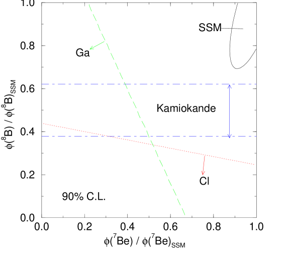
Fig. 2: The allowed fluxes when the Homestake, Kamiokande, and the gallium results are fit separately. This is an updated analysis of Ref. [[28]].

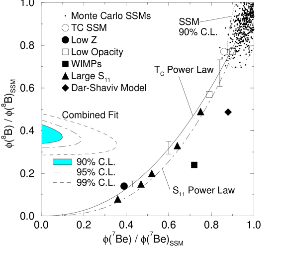
Fig. 3: The fluxes allowed by the combined data. Also shown are various standard and nonstandard solar models. This is an updated analysis of Ref. [[28]].

When each experiment is fit separately, the Kamiokande data constrain the ⁸B flux, and the Homestake and gallium experiments constrain both the ⁷Be and ⁸B fluxes; constraints at the 90% C.L. from each experiment are shown in Fig. 2. In this model $\phi(\mbox{Be})=\phi(\mbox{B})=0$ is completely consistent with the Homestake and gallium observation, since we can always adjust the $pp$ and CNO fluxes to the observed rates. As seen in Fig. 2, each of the experiments is inconsistent with the SSM prediction.

When the observations are fit combined, astrophysical solutions in general are excluded, and the argument comes in three steps.

The $\chi^{2}$ value of the joint fit is very poor. In fact if (nonphysical) negative fluxes were allowed, the $\chi^{2}$ minimum is obtained for $\phi(\mbox{Be})/\phi(\mbox{Be})_{\mbox{\scriptsize SSM}}\sim-0.5$. Within the physical region, the best fit is obtained for $\phi(\mbox{Be})/\phi(\mbox{Be})_{\mbox{\scriptsize SSM}}<0.08$ and $\phi(\mbox{B})/\phi(\mbox{B})_{\mbox{\scriptsize SSM}}=0.37\pm 0.04$ (1$\sigma$), but only with $\chi^{2}=4.1$ for 1 d.f. Statistically this fit is excluded at 96% C.L. In other words, any astrophysical solutions consistent with our minimal assumptions are excluded at 96% C.L. by the observations.

Secondly, even if I allow the 4% chance and accept the solution, the obtained fluxes do not physically make sense at all. Since ⁸B is produced by the reaction $p+{}^{7}\mbox{Be}\rightarrow{}^{8}\mbox{B}+\gamma$, essentially any reduction in the ⁷Be flux should cause at least an equal reduction in the ⁸B flux, and additional temperature sensitivity reduces the ⁸B flux more. Therefore, unless the uncertainty of the ⁷Be electron capture rate is grossly underestimated or there is some independent mechanism to suppress only the ⁷Be neutrinos, any realistic model should be in the region $\phi(\mbox{Be})/\phi(\mbox{Be})_{\mbox{\scriptsize SSM}}\geq\phi(\mbox{B})/\phi(\mbox{B})_{\mbox{\scriptsize SSM}}$ in Fig. 3, contrary to the observations.

Finally various standard and nonstandard solar models are plotted in Fig. 3. The Bahcall-Pinsonneault SSM with 90% C.L. uncertainty [1], the Bahcall-Ulrich 1000 Monte Carlo SSMs [29], the Turck-Chièze–Lopes SSM [2], the solar models with opacity reduced by 10 and 20% [34], the large $S_{11}$ models by Castellani et al. [35], the low Z model by Bahcall and Ulrich [29, 30], the WIMP model by Gilliland et al. [36, 30], and the Dar-Shaviv model [19]. Also shown are the power law dependence of the fluxes to $T_{C}$ and $S_{11}$ obtained by Bahcall and Ulrich [29, 30]. None of those models is even close to the observations.

This complete failure of our model forces us to conclude that at least one of the original assumptions is wrong. We have repeated the analysis without the luminosity constraint; the exclusion of the model is somewhat weaken (the exclusion is at 95% C.L.), but the conclusion remains essentially the same. Therefore we have to conclude that either of the other two assumptions is incorrect: (a) there is a distortion of the ⁸B flux, that is, new neutrino physics, or (b) one or more of the experiments is wrong: in particular, either the Homestake or Kamiokande data must be grossly wrong.

2.3 What if Homestake data were ignored?

As discussed in the previous section, the most compelling motivation for the particle physics solutions such as the MSW effect comes from the comparison of the Homestake and Kamiokande data, and, if one of the two were ignored, the astrophysical solutions cannot be dismissed outright. Some argue that we would lose motivations for new neutrino physics if the Homestake data were ignored. This, however, is misleading: at present we have no realistic solar model that are consistent both with the Kamiokande and gallium results within their uncertainties.

I address the issue by considering the solar models with the ⁸B flux consistent with the observed Kamiokande rate [42]. The Monte Carlo SSMs with such a constraint were discussed in Ref. [[25]], but I also allow nonstandard solar models. The neutrino flux varies significantly from model to model in nonstandard solar models in general, but the fact that about half of the SSM ⁸B flux is seen strongly constrains the nonstandard solar models, and yields predictions for the gallium rate and the helioseismology observations. I list in Fig. 4 the expected gallium rates from various nonstandard models that are consistent with or close to the ⁸B flux observed by Kamiokande: the model in which $S_{17}$ is adjusted from the Bahcall-Pinsonneault model to the observed Kamiokande rate ($0.51\pm 0.07$ SSM), the low $T_{C}$ model, the low $T_{C}$ model with $S_{17}$ increased by 30%, the model with $S_{34}$ reduced to the Kamiokande rate, the Dar-Shaviv model [19], the low opacity model ($-$20%) [34], the model with $S_{11}$ increased by 30% [35] and 25% [2], and the mixing models by Sienkiewicz et al [40]. The uncertainties include the uncertainty of the ⁸B flux due to the Kamiokande uncertainty (14%), but the dominant contribution is from the gallium cross section uncertainty. From this list, I obtain

$$\mbox{Gallium rate consistent with Kamiokande}\geq 100\;\mbox{SNU},$$ (5)

while the combined gallium rate of SAGE and GALLEX is 78 $\pm$ 10 SNU.

Fig. 4: The rate of the gallium experiments, the gallium rates of the SSMs, and of the nonstandard solar models which predict the ⁸B flux consistent with or close to the flux observed in Kamiokande. See text for details. The nonstandard solar models consistent with Kamiokande predict the gallium rate $R_{\mbox{\scriptsize Ga}}>$ 100 SNU. The MSW solution obtained from the combined Kamiokande and Homestake data predicts $R_{\mbox{\scriptsize Ga}}<$ 100 SNU, consistent with the data.

Obviously it is still premature to rule out those nonstandard solar models given the current large experimental uncertainties. But the observations and the theoretical predictions are showing discrepancies. Also other solar observations might exclude those models. The helioseismology observations provide information on the sound speed throughout the radiative and convective zone (but not in the core region where the theoretical and experimental uncertainties are still large). As discussed by other speakers at this conference, the observations give significant constraints in solar model building: the SSM is consistent with the helioseismology data at the 1% level, and any large departures from the SSM will be likely to destroy this agreement. In fact, some of the nonstandard solar models listed in Fig. 3 and also other nonstandard models such as the low $T_{C}$ model [43], the large $S_{11}$ model [2], the mixing model [41], and the low Y model [43] are in conflict with the helioseismology observations.

While waiting for the gallium detectors to be calibrated and the statistics of the gallium data to improve, this line of theoretical investigations should be encouraged. I hope that the possibility of solar models consistent with the Kamiokande and the gallium data will be pursued, and the list of nonstandard models as in Fig. 3 will be extended to obtain the minimum rate expected for the gallium experiments. Also, each and every model should be confronted with the helioseismology observations. If one could successfully find a model consistent with the Kamiokande and gallium as well as the helioseismology observations, it could be the solution to the solar neutrino problem: the SSM and the Homestake experiment might be wrong after all. If, however, one could not find such a model after entirely discarding the Homestake data, our motivation for considering particle physics solutions will be complete.

3 MSW Solutions

There are many proposed particle physics solutions to the solar neutrino problem: the MSW effect with two or more flavors, vacuum oscillations, a large neutrino magnetic moment, neutrino decays, violations of the equivalence principle, etc. I discuss the two state MSW oscillations [45], since it requires only the minimal extension of the standard model (mass and mixing of neutrinos) without contradicting with any other existing observational constraints, and also without requiring any unnatural fine-tunings of the parameters. Furthermore, many extensions of the standard electroweak model with the see-saw mechanism [44] suggest neutrino mass consistent with the MSW parameter range [46], providing a theoretical motivation to look for neutrino mass in the solar neutrino experiments. I also consider the MSW oscillations for sterile neutrinos and the MSW solutions in the context of nonstandard solar models. The MSW analysis of the solar neutrino data was carried out by many authors [47, 48, 49, 50, 51, 52, 53], but here I follow the recent analysis of Ref. [[24, 54, 31]], which includes the theoretical uncertainties and their correlations, the Earth effect, the Kamiokande II day-night data, and the improved definition of the confidence levels.

3.1 Earth Effect

One interesting, but not-well publicized, aspect of the MSW mechanism is the Earth effect [55] on the solar neutrinos. The electron neutrinos produced in the Sun transform to another species of neutrino by the MSW effect in the Sun, but, for a certain parameter range, they can transform back to $\nu_{e}$’s during the night due to the matter effect as the neutrinos propagate through the Earth. Such an effect can be seen as a difference in the observed rate between day and night, or, more drastically, as signal variations as a function of time during the night since the oscillation probabilities depend sensitively on the neutrino path length in the Earth and also on the densities that the neutrino go through (i.e., the mantle only or both the mantle and the core). The Earth effect is only relevant for a limited region of $\Delta m^{2}$ and $\sin^{2}2\theta$, but, if measured, it would be an indisputable evidence for the MSW solution. Given the high statistics in the next generation experiments, the MSW parameters ($\Delta m^{2}$ and $\sin^{2}2\theta$) could be determined precisely by measuring time and energy dependence. Since the measurement depends only on the time (and energy) dependence, but not on the absolute neutrino flux, the determination of $\Delta m^{2}$ and $\sin^{2}2\theta$ would be free from the solar model uncertainties and also from the time-independent systematic uncertainties in the experiments; the uncertainties from the Earth density profile is negligibly small.

The MSW transition is most significant when the resonance condition is satisfied:

$${\Delta m^{2}\over 2E}\cos 2\theta=\sqrt{2}\,G_{F}\,n,$$ (6)

where $E$ is the neutrino energy, $G_{F}$ is the Fermi constant; $n=n_{e}$ for oscillations to $\nu_{\mu}$ or $\nu_{\tau}$, and $n=n_{e}-n_{n}/2$ for oscillations to sterile neutrinos, where $n_{e}$ and $n_{n}$ are the electron and neutron densities. The density profile of the Earth is approximately described as two step functions: the core (10 – 12.5 g/cm³) and the mantle (4 – 5 g/cm³). A more detailed density profile can be found in Ref. [[56]]. For solar neutrinos energies, the parameter space relevant for the Earth effect is $\Delta m^{2}\sim 10^{-7}-10^{-5}\;\mbox{eV}\;^{2}$ and $\sin^{2}2\theta\geq 0.01$. To compare the MSW predictions to the averaged rates of observations, one needs to average the $\nu_{e}$ survival probability over the night, since it depends on the path length and also on the density profile through which the neutrinos propagate. The survival probability also vary each night due to the obliquity of the Earth rotation axis and should be averaged over a year. Also it differs for each experiment due to the detector latitudes. This averaging process requires intensive computations.

The contours of the signal-to-SSM ratio for the Kamiokande experiment are shown in Fig. 5 for the day-time rate (a) and the night-time rate (b). For a certain parameter space, the night-time enhancement is huge: for example, the night-time rate is almost three times the day-time rate for $\Delta m^{2}\sim 3\times 10^{-6}\;\mbox{eV}\,^{2}$ and $\sin^{2}2\theta\sim 0.2$.

(a) Day-time rate

(b) Night-time rate

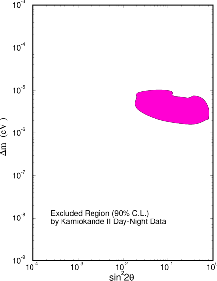
(c) Kam II day-night data

Fig. 5: The contours of the signal-to-SSM ratio in Kamiokande for (a) day time and (b) night time. (c) Also shown is the region excluded by the Kamiokande II day-night data with 6 time bins.

Real-time counting experiments such as Kamiokande are capable of observing the day-night effect. In fact the Kamiokande II collaboration has published the day-night data with 6 bins (one day-time data point and 5 night-time data points for different angles between the Sun direction and the nadir at the detector; the binning corresponds to selecting neutrinos with different path lengths in the Earth). The data show no enhancement of the signal at night, albeit still large statistical uncertainties, and exclude the parameter space shown in Fig. 5 (c). This exclusion of parameter space is insensitive to the solar model uncertainties and independent of solar models.

The Earth effect has significant phenomenological implications to the existing and future direct-counting experiments. The day-night data are available so far only from the Kamiokande II experiment. The additional data from Kamiokande III is expected to double the statistics, and the updated analysis should further constrain the parameter space. In particular, a significant day-night effect is expected in the large-angle solution of the combined observations, which might be observable if the Kamiokande II data and the (still unpublished) Kamiokande III day-night data are combined. With large counting rates in the future solar neutrino experiments, one should be able to observe a day-night effect at a few per cent level, and the parameter space in which the contours in Fig. 5 (b) are distorted from Fig. 5 (a) should produce observable signals. If the day-night effect is observed, its time and energy dependence provides a clean determination of $\Delta m^{2}$ and $\sin^{2}2\theta$ without referring to solar model calculations. The detailed predictions of the day-night effect for SNO, Super-Kamiokande, and Kamiokande obtained from the MSW solutions of the combined observations will be given in Section 3.6.

3.2 MSW Analysis

Given a solar model, either standard or nonstandard, the MSW mechanism is a solid, calculable theory. It can be quantitatively tested and constrained, and the following is the questions to be addressed in the MSW analysis:

1. Is the MSW hypothesis acceptable by the observations?

2. If acceptable, what is the parameter space allowed by the observations?

3. What are the predictions for the future experiments from the obtained parameters?

The first question tests the whole idea of the MSW theory, including the assumption of neutrino mass and mixing. The answer to the second question will provide important information for the neutrino mass spectrum and mixing matrix of the lepton sector. And most importantly, the MSW theory is verifiable or falsifiable by the next generation experiments.

To answer those questions quantitatively, it is important to include relevant theoretical uncertainties in the analysis. Especially the ⁸B flux uncertainty in the Bahcall-Pinsonneault SSM is 14% and comparable to the experimental uncertainties of Homestake (11%) and Kamiokande (14%). In the Turck-Chièze –Lopes SSM, the ⁸B flux uncertainty is 25% and dominates the experimental uncertainties.

Equally important, but often ignored, are the correlations among the theoretical uncertainties. The leading uncertainty from the ⁸B flux is strongly correlated among the experiments, especially between Homestake and Kamiokande. Also the uncertainties are correlated between different flux components. If, for example, the opacity were lower (or the core temperature were lower), both the ⁷Be flux and ⁸B flux would be reduced. Therefore a careful estimation of the theoretical uncertainties and their correlations are essential in determining the neutrino parameters. In fact if the theoretical uncertainties were ignored, there would be no allowed solution in the large-angle region at 90% C.L. If the correlations were ignored, a significantly larger region would be obtained for the large-angle solution [31].

We have parameterized the SSM flux uncertainties by the uncertainties in the central temperature and in the relevant nuclear reaction cross sections ($S_{17}$ and $S_{34}$) [31, 24, 54]. It was shown explicitly that our treatment reproduces the flux uncertainties and correlations obtained from the Bahcall-Ulrich 1000 Monte Carlo SSMs [31]. The parameterization method can be easily generalized to other solar models, for which the Monte Carlo estimations are unavailable. The ⁷Be and ⁸B flux distributions of the Bahcall-Ulrich 1000 Monte Carlo SSMs and our parametrized uncertainty estimation are displayed in Fig. 6. The amplitudes and the correlation of the flux uncertainties are consistent between the two methods.

Fig. 6: The ⁷Be and ⁸B flux distributions of the Bahcall-Ulrich 1000 Monte Carlo SSMs (dots). Also shown (solid line) are the flux uncertainties (at 90% C.L.) parametrized by the central temperature and the relevant nuclear cross sections. The two methods provide consistent flux uncertainty estimations. Taken from Ref. [[31]].

One ambiguity in determining the neutrino parameters is the definition of confidence levels. The general prescription in this case is that, once the MSW mechanism is accepted as a viable solution, the probability density of the parameter space allowed by the observations is distributed throughout the $\log\Delta m^{2}-\log\sin^{2}2\theta$ plane, and is given as $P=N\exp(-\chi^{2}/2)$, where $N$ is the normalization factor and the $\chi^{2}$ is calculated for each combination of $\Delta m^{2}$ and $\sin^{2}2\theta$ [31]. When the probability distribution is approximated as a gaussian around the $\chi^{2}$ minimum, the allowed region is determined by $\chi^{2}(\Delta m^{2},\sin^{2}2\theta)\leq\chi^{2}_{\mbox{\scriptsize min}}+\Delta\chi^{2}$ with $\Delta\chi^{2}$ = 4.6, 6.0, and 9.2 for 90, 95, and 99% C.L., respectively. The $\Delta\chi^{2}$ is determined by the fact that the probability density is distributed in the 2-dimensional parameter space, and does not depend on the number of data points which enter the $\chi^{2}$ calculation. The assumption of one gaussian distribution is questionable for the MSW analysis, which yields multiple $\chi^{2}$ minima in the parameter space. We have generalized the $\Delta\chi^{2}$ method in the presence of multiple $\chi^{2}$ minima [31], and will use the improved definition in the joint analysis.

We use the Petcov formula [57, 58] to calculate the $\nu_{e}$ survival probability, and have compared the results to other analytic approximations (the Parke formula with the Landau-Zener approximation [59] and the Pizzochero formula [60]), and found that the difference in the combined fit is completely negligible. Also our calculations were compared to those of Fiorentini et al. [53], who solve the neutrino propagation equation numerically: the agreement was excellent.

Our MSW calculations include the MSW double-crossing, the neutrino production distributions in the Sun [1], the electron density distribution [1], the detector cross sections [29, 30], and the energy resolution and the detector efficiency for Kamiokande [5].

The uncertainties from the neutrino production distributions and from the electron density distributions are studied by comparing three different solar models (but using the same flux magnitude) [31]: the Bahcall-Ulrich SSM and the Bahcall-Pinsonneault SSM with and without the helium diffusion effect. No difference was observed. We have also changed by $\pm$10% each the peak location of the production distribution, the electron density scale height, and the core-mantle boundary in the Earth, which enters into the Earth effect calculation; the combined solutions were insensitive to the changes [31].

3.3 Updated Results

The updated MSW results including the most recent GALLEX, SAGE, and Kamiokande III data are presented in Fig. 7 (a). The joint fit includes the Homestake, combined gallium, Kamiokande II day-night data (6 data points) and the Kamiokande III data. We have incorporated the Earth effect, the theoretical and experimental uncertainties and their correlations. The Bahcall-Pinsonneault SSM with helium diffusion effect is assumed unless otherwise mentioned. The improved confidence level definition is robust under the assumption that the probability density is distributed throughout the parameter space and the distribution is described as a multiple gaussian distribution, i.e., the allowed regions should have an elliptic shape, which is a good approximation in our case. Fig. 7 (b) shows the combined allowed regions for 90, 95, and 99% C.L. Note that there is a third allowed region for $\Delta m^{2}\sim 1.2\times 10^{-7}\,\mbox{eV}\,^{2}$ and $\sin^{2}2\theta\sim 0.8$, but only at 99% C.L.; this region is disfavored by the Kamiokande II day-night data and also by the combined result of GALLEX and SAGE.

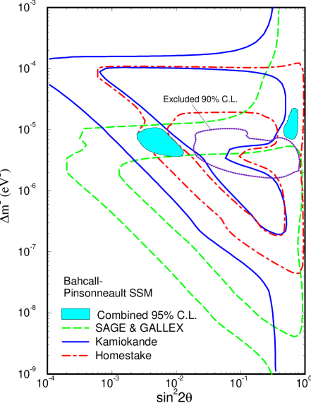
(a) Combined results

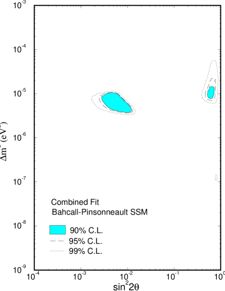
(b) 90, 95, and 99% C.L.

Fig. 7: (a) The MSW solutions allowed at 95% C.L. by the combined observations of the Homestake, the combined gallium SAGE and GALLEX, the Kamiokande II including six day-night data points, and the Kamiokande III data. Also shown are the regions allowed by each of the experiments and the region excluded by the Kamiokande II day-night data (dotted line). (b) The combined allowed regions at 90, 95, and 99% C.L. This is an updated analysis of Ref. [[31]].

Table 3: The best fit parameters of the combined MSW solutions.

	Nonadiabatic	Large Angle I	Large Angle II
$\sin^{2}2\theta$	$6.8\times 10^{-3}$	0.62	0.80
$\Delta m^{2}$ (eV2)	$6.2\times 10^{-6}$	$9.7\times 10^{-6}$	$1.3\times 10^{-7}$
$\chi^{2}$ (7 d.f.)	2.4	6.9	12.7
G.O.F.(%)	94	44	8
$P_{\mbox{\scriptsize relative}}$ (%)	92.2	7.5	0.3

The best fit parameters, $\chi^{2}$ values, the goodness-of-fit (G.O.F), and relative probabilities are listed for each solution in Table 3. G.O.F is the probability of obtaining by chance a $\chi^{2}$ value equal to or larger than the obtained $\chi^{2}$. The relative probability is the probability of finding the true solution in this region when the probability density is assumed to be a gaussian distribution for each solution [31].

Note that the small-angle (nonadiabatic) solution provides an excellent fit: the MSW solution is an acceptable theory by the combined observations. In fact $\chi^{2}=2.4$ for 7 d.f. (9 data points – 2 parameters) is too good. This is due to a small contribution from the Kamiokande II 6 day-night data point ($\chi^{2}\sim 2.1$), and without the day-night data, the $\chi^{2}/$1 d.f. is 0.3 (58% C.L.), which is reasonable.

Compared to the small-angle (nonadiabatic) solution, the two large-angle solutions are disfavored by the observations. This is due to the characteristic energy dependence of the solutions shown in Fig. 8. For the small-angle (nonadiabatic) solution, the ⁷Be neutrinos and the lower energy part of the ⁸B neutrinos are suppressed, consistent with the observed relative rates of Homestake and Kamiokande. On the other hand, the energy dependence for the large angle solution is mild, and the central values of Homestake and Kamiokande cannot be simultaneously given by the MSW effect. This is similar to the reason why the astrophysical solutions are disfavored, but is less severe: in the large-angle MSW case, the converted $\nu_{\mu}$ or $\nu_{\tau}$ can still interact in the Kamiokande detector via the neutral current interaction (with about 1/6 the cross section), reducing the inferred $\nu_{e}$ survival probability to a value close to that of Homestake. There is also a slight enhancement of the survival probability at larger energies due to the Earth effect.

Fig. 8: The energy dependence of the two MSW solutions allowed by the combined observations. The small-angle (nonadiabatic) solution gives a better fit than the large-angle solution. The survival probability depends on the neutrino production distribution, and the plot assumes the distribution of the ⁸B neutrinos, which is concentrated around the center of the Sun. The survival probability for the two ⁷Be lines is essentially the same; for the $pp$ neutrinos, the production region is more wide spread, and consequently the decrease of the survival probability around $E\sim 0.5$ MeV is less steep.

The MSW oscillations also can be considered for sterile neutrinos, and the allowed parameter space is displayed in Fig. 9. There is no allowed large-angle region even at 99% C.L., since the absence of the neutral current events in Kamiokande makes the $\nu_{e}$ survival probabilities effectively larger than for flavor oscillations. The large-angle regions are therefore strongly disfavored, much like the astrophysical solutions. The exclusion of the large-angle region for sterile neutrinos has been independently obtained from neutrino counting in big-bang nucleosynthesis [61].

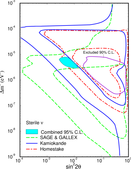
Fig. 9: The parameter space allowed for oscillations for sterile neutrinos. There is no allowed regions for large angles even at 99% C.L., which is consistent with the big-bang nucleosynthesis constraint. Taken from Ref. [[31]].

The MSW regions for the Turck-Chièze–Lopes model is displayed in Fig. 10. This model does not include the particle diffusion effect, and also the neutrino production distributions and the electron density distributions have not been published. The calculation is done by using those of the Bahcall-Pinsonneault model. The obtained allowed regions are slightly shifted outward of the MSW triangle compared to the Bahcall-Pinsonneault solutions due to the smaller predicted fluxes. Also the allowed regions are noticeably larger, reflecting that the flux uncertainties are more conservative in the Turck-Chièze–Lopes SSM. Therefore the correct uncertainty estimation is important in constraining neutrino parameters, and underestimation of the flux uncertainties can lead to underestimation of the uncertainties of $\Delta m^{2}$ and $\sin^{2}2\theta$.

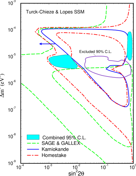
Fig. 10: The allowed parameter space when the Turck-Chièze–Lopes SSM is assumed. Taken from Ref. [[31]].

3.4 MSW in Nonstandard Solar Models

The SSM is assumed in the MSW analysis discussed in the previous section. Even if the MSW is proven, however, that does not confirm that the SSM is correct; the MSW effect can also take place in the nonstandard solar models. The SSM is still needs to be tested and calibrated experimentally. To address such a possibility, we have carried out the MSW analysis while the core temperature is allowed to change freely. The neutrino fluxes are changed according to the power law obtained by Bahcall and Ulrich (Eqn. 1), except that the $T_{C}$ dependence of the pp flux is obtained from the luminosity constraint (Eqn. 2). From a three parameter fit ($\Delta m^{2}$, $\sin^{2}2\theta$, and $T_{C}$), we constrained

$$T_{C}=1.02\pm 0.02\hskip 5.0pt(1\sigma),$$ (7)

with $\chi^{2}_{\mbox{\scriptsize min}}=2.1$ for 6 degrees of freedom (d.f.), where $T_{C}$ is in units of the Bahcall-Pinsonneault SSM ($15.57\times 10^{6}\;\mbox{K}$). Interestingly the existing observations constrain the central temperature of the Sun at the 2% level even in the presence of the MSW effect. (Note that there is no consistent $T_{C}$ to describe the observations without the MSW effect. See Section 2.1.) Also the value obtained for $T_{C}$ is consistent with the Bahcall-Pinsonneault SSM value $T_{C}=1\pm 0.006$. If the MSW is proven, the above will be the first observational constraint on the core temperature of the Sun at the 2% level. The combined MSW regions with free $T_{C}$ are shown in Fig. 11.

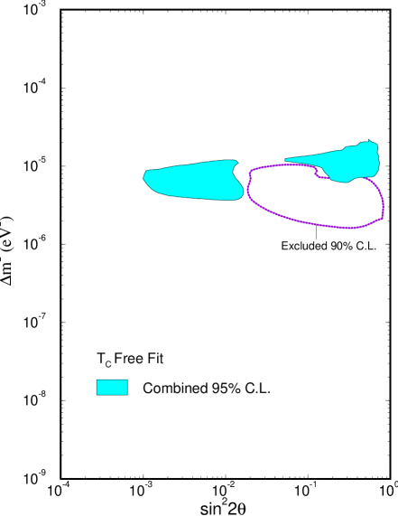
Fig. 11: The allowed parameter space when the central temperature is allowed to change freely. The data constrain $T_{C}=1.02\pm 0.02\;(1\sigma)$. Taken from Ref. [[31]].

Since the ⁸B flux has the largest uncertainty (14% in the Bahcall-Pinsonneault SSM and 25% in the Turck-Chièze–Lopes model), we have also carried out the analysis with the ⁸B flux as a free parameter. The constraint obtained from the observations is weak, but consistent with the SSM:

$$\phi(\mbox{B})/\phi(\mbox{B})_{\mbox{\scriptsize SSM}}=1.43+0.65-0.42\;(1\sigma).$$ (8)

The allowed regions for this case is shown in Fig. 12.

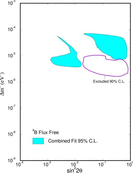
Fig. 12: The allowed parameter space when the ⁸B flux is used as a free parameter. Taken from Ref. [[31]].

We have also considered the MSW solutions for nonstandard solar models that are explicitly constructed, and the results are shown for four nonstandard solar models in Fig. 13. Two of them predict smaller initial fluxes compared to the SSM: the low opacity model [34] and the large $S_{11}$ model [35]. The other two predict larger fluxes than the SSM: the high Y model [29] and the maximum rate model [1]. With nonstandard input parameters or nonstandard core temperatures, a wider MSW parameter space is allowed.

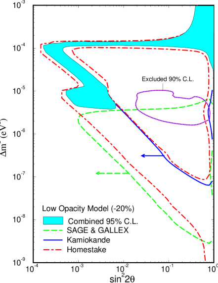
(a) Low opacity

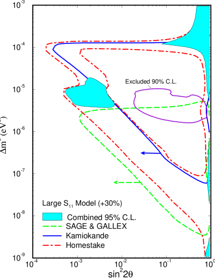
(b) Large $S_{11}$

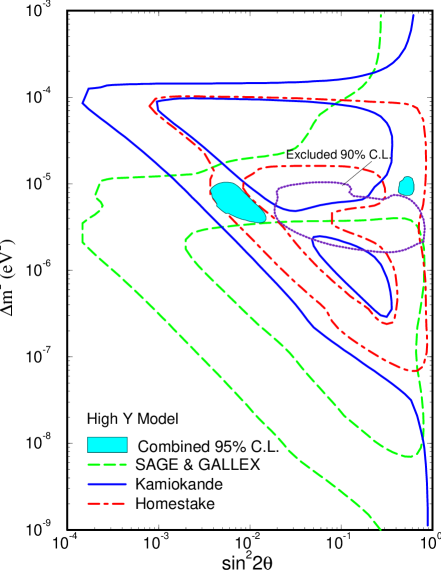
(c) High Y model

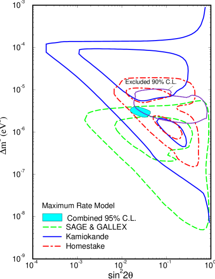
(d) Maximum rate model

Fig. 13: The allowed parameter space for nonstandard solar models: (a) the low opacity model and (b) the large $S_{11}$ model predict smaller neutrino fluxes than the SSM, while (c) the high Y model and (d) the maximum rate model predict larger fluxes. Taken from Ref. [[31]].

Among the above nonstandard solar models, the maximum rate model and the large $S_{11}$ model are significantly different from the SSM, and are disfavored by the solar neutrino data even with the MSW effect. But nonstandard core temperature within $T_{C}\sim 1-1.04$ is perfectly consistent with the observation. A further constraint on $T_{C}$ (or the neutrino flux) from the helioseismology observations is welcome.

3.5 Observational Constraints and Hints for Neutrino Mass and Mixing

There are two observational hints of neutrino mass other than solar neutrinos: the oscillation interpretation of the atmospheric neutrino deficit [62], and the cold plus hot dark matter scenario for the cosmic background radiation measurements and the large-scale structure observations [63]. The parameter ranges for those hypotheses are displayed in Fig. 14, along with the MSW and vacuum oscillation solutions [64] of the solar neutrino problem. The constraints from the oscillation experiments [65] and the constraints for oscillations to sterile neutrinos from big-bang nucleosynthesis [66] are also shown.

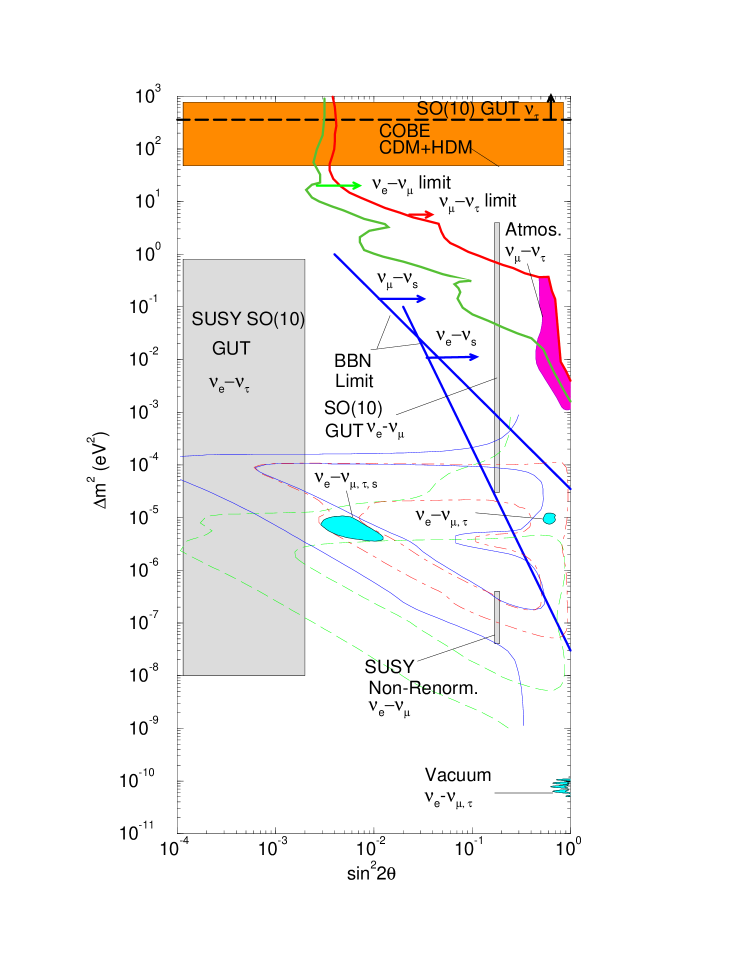
Fig. 14: Various observational constraints and hints for neutrino mass and mixing. Also shown are various theoretical predictions. See text for details.

Fig. 14 also shows the parameter space of various theoretical predictions involving the see-saw mechanism [44]: the $\nu_{e}-\nu_{\mu}$ mixing in the $SO_{10}$ grand unified theory (GUT) with an intermediate scale breaking [23, 46], the $\nu_{e}-\nu_{\tau}$ mixing in the supersymmetric $SO_{10}$ GUT [23, 46], and the $\nu_{e}-\nu_{\mu}$ mixing in the superstring-inspired model with nonrenormalizable operators [67] (there is no compelling prediction for the mixing angles for this model). The mixing angles shown for these theories (Fig. 14) are the corresponding quark mixing angles ($V_{\mbox{\scriptsize lepton}}\sim V_{\mbox{\scriptsize CKM}}$). In the $SO_{10}$ GUT, the $\nu_{\tau}$ mass is expected to be in a range relevant to the cosmological hot dark matter. The detailed mass range and mixing angles are model dependent, and can be different from what is shown. The general idea of grand unification and the see-saw mechanism suggests the neutrino mass scales shown in Fig. 14, and there is a solid motivation to look for neutrino mass in the MSW range relevant for solar neutrinos.

The next question is whether this picture is reality, or just a fantasy of particle physicists, and, more importantly, whether we can prove or disprove such theoretical ideas. For solar neutrinos, experimental quests are directly aiming at the detection of neutrino oscillations, and the next generation experiments of the Sudbury Neutrino Observatory (SNO), Super-Kamiokande, BOREXINO, and ICARUS should either confirm or rule out the neutrino oscillation hypothesis. For other neutrino mass ranges, two accelerator-based oscillation experiments at CERN (CHORUS and NOMAD) will start operating in the spring of 1994, and explore the cosmologically interesting $\nu_{\tau}$ mass range down to small mixing angles ($\Delta m^{2}>1-10\;\mbox{eV}\,^{2}$ and $\sin^{2}2\theta<2\times 10^{-4}$ for $\nu_{\mu}\leftrightarrow\nu_{\tau}$ oscillations). The proposed long-baseline experiments of Brookhaven and Fermilab-SOUDAN will explore the parameter space suggested by the atmospheric neutrino deficit.

3.6 MSW Predictions for Future Experiments

As discussed in the previous sections, we have compelling reasons to consider the MSW mechanism as a solution to the solar neutrino problem: a lack of viable astrophysical explanations provides a strong motivation for particle physics solutions, while the data are consistent with the MSW descriptions; the idea of GUTs and the see-saw mechanism suggests a neutrino mass range consistent with the MSW solutions.

It is still premature, however, to convince ourselves that neutrino mass and mixing are the cause of the solar neutrino deficit. More data are needed, and the next generation experiments such as SNO [68], Super-Kamiokande[69], BOREXINO [70], and ICARUS [71] should provide a definitive answer for neutrino oscillation hypothesis. There are two theoretical questions which should be answered by the new experiments.

• Calibrate the solar model. The neutrino flux should be determined component by component from experimental data.

• Determine the solution and the parameter space. In particular distinguish the MSW solutions from astrophysical solutions and also from other particle physics solutions, and constrain $\Delta m^{2}$ and $\sin^{2}2\theta$.

The procedure of doing these can be complicated, since the the determination of the neutrino parameters depends on the neutrino flux and, in turn, the determination of the neutrino flux requires a knowledge of the neutrino parameters. These can be accomplished by the next generation experiments with high counting rates and various reaction modes. The reaction modes of the experiments with projected counting rates are summarized in Table 4.

Table 4: The future solar neutrino experiments. CC, NC, and ES stand for charged current, neutral current, and elastic scattering mode.

Experiment	Commission date	Reaction mode	Event rate
SNO	Fall, 1995	CC: $\nu_{e}+d\rightarrow p+p+e^{-}$	3,000 events/yr
		NC: $\nu_{e,\mu,\tau}+d\rightarrow\nu_{e,\mu,\tau}+p+n$	3,000 events/yr
		ES: $\nu_{e,\mu,\tau}+e^{-}\rightarrow\nu_{e,\mu,\tau}+e^{-}$	200 events/yr
Super-Kamiokande	April, 1996	ES: $\nu_{e,\mu,\tau}+e^{-}\rightarrow\nu_{e,\mu,\tau}+e^{-}$	8,000 events/yr
BOREXINO	Late 1990’s	ES (7Be): $\nu_{e,\mu,\tau}+e^{-}\rightarrow\nu_{e,\mu,\tau}+e^{-}$	18,000 events/yr (SSM)
ICARUS	$\sim$ 2000	ES: $\nu_{e,\mu,\tau}+e^{-}\rightarrow\nu_{e,\mu,\tau}+e^{-}$	2,900 events/yr/module
		CC: $\nu_{e}+{}^{40}\mbox{Ar}\rightarrow{}^{40}\mbox{K}^{*}+e^{-}$	2,400 events/yr/module
Iodine	Late 1990’s	CC: $\nu_{e}+{}^{127}\mbox{I}\rightarrow{}^{127}\mbox{Xe}+e^{-}$

Given the current data and the SSM, one can yield robust predictions for future experiments to test the MSW hypothesis. The MSW mechanism provides a solid, calculable theoretical frame work; the theoretical uncertainties are, by and large, under control. The predictions include the charged to neutral current ratio, the spectrum distortions, and the day-night difference. The charged to neutral current ratio (CC/NC) is the gold-plated measurement in SNO of confirming neutrino oscillations; however, whether SNO can distinguish the MSW solution from astrophysical solutions at the $3\sigma$ level is solar model dependent; if the ⁸B flux is smaller by 20% than that of the Bahcall-Pinsonneault SSM, the MSW solution may not be established given the projected systematic uncertainty of $\sim$ 20%. On the other hand, energy spectrum distortions and the day-night effect are completely free from the solar model uncertainties and theoretically clean observables. By requiring consistency among those measurements from different experiments, we should be able to determine the solution and constrain the parameter space with a sufficient precision.

3.6.1 CC/NC Measurement in SNO

Measuring a depletion of the charged current (CC) rate with respect to the neutral current (NC) rate in SNO is considered to be the smoking gun evidence to establish neutrino oscillations. From the global solutions assuming the Bahcall-Pinsonneault SSM [Fig. 15 (a)] at 95% C.L., the ratio (CC/NC) is expected to be

$$\frac{\mbox{(CC/NC)}_{\mbox{\scriptsize SNO}}\hskip 8.99994pt}{\mbox{(CC/NC)}_{\mbox{\scriptsize No Osc}}}=\left\{\begin{array}[]{ l l }0.2-0.65&\mbox{ (Nonadiabatic Solution) }\\ 0.2-0.3&\mbox{ (Large-Angle Solution), }\end{array}\right.$$ (9)

where (CC/NC)${}_{\mbox{\scriptsize No Osc}}$ is the ratio expected for no oscillations or for oscillations into sterile neutrinos. This prediction is, however, solar model dependent. Using the Turck-Chièze–Lopes model, which predicts a smaller ⁸B flux with a larger uncertainty, the prediction [Fig. 15 (b)] becomes

$$\frac{\mbox{(CC/NC)}_{\mbox{\scriptsize SNO}}\hskip 8.99994pt}{\mbox{(CC/NC)}_{\mbox{\scriptsize No Osc}}}=\left\{\begin{array}[]{ l l }0.2-0.85&\mbox{ (Nonadiabatic Solution) }\\ 0.2-0.4&\mbox{ (Large-Angle Solution). }\end{array}\right.$$ (10)

I emphasize that the prediction of whether SNO can distinguish the MSW solutions from astrophysical solutions by the CC/NC measurement is strongly dependent on the ⁸B flux and its uncertainty used in obtaining the current MSW solutions. With the current projection of systematic uncertainty at the 20% level, the distinction with a 3$\sigma$ significance is achievable assuming the Bahcall-Pinsonneault SSM. It is no longer guaranteed if the Turck-Chièze–Lopes SSM is assumed. Given the large uncertainty in the $S_{17}$ determination, a ⁸B flux smaller by 20% than that of the Bahcall-Pinsonneault SSM is a distinct possibility. Furthermore, there are additional uncertainties in other inputs such as opacity calculations. It is emphasized that the solar model uncertainties can affect the predictions for future experiments, and especially the SNO experiment development can be affected by future improvements in the $S_{17}$ determination.

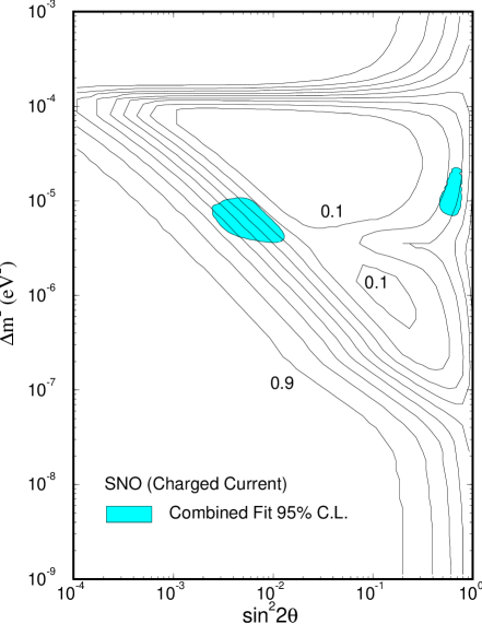
(a) Bahcall-Pinsonneault SSM

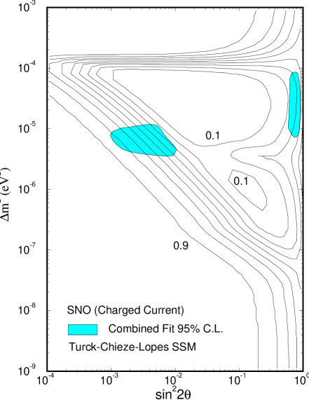
(b) Turck-Chièze–Lopes SSM

Fig. 15: The contours of the signal-to-SSM ratio for the SNO charged current measurement with the combined allowed region assuming (a) the Bahcall-Pinsonneault SSM and (b) the Turck-Chièze–Lopes SSM. This is an updated result of Ref. [[31]].

3.6.2 Spectrum Distortions

The ⁸B spectrum measurements in SNO, Super-Kamiokande, and ICARUS provide a unique opportunity to look for energy dependent effects on low energy neutrinos with an unprecedented precision. Astrophysical effects on the spectrum such as from gravitational red-shifts and thermal fluctuations are completely negligible at the observable level [33], while particle physics effects (or new neutrino physics) is often energy dependent, and spectrum distortions are a theoretically clean signal for new physics. In particular the MSW small-angle (nonadiabatic) solution predicts spectrum distortions, suppressing the lower energies of the ⁸B flux more. The spectrum shapes predicted by the global MSW solutions are displayed in Fig. 16 for SNO (charged current reaction) and Super-Kamiokande. The error bars correspond to statistical uncertainties from 6,000 and 16,000 events, respectively (equivalent to 2 years of operation). To compare differences in the shape, the large-angle spectrum is normalized to the small-angle (nonadiabatic) spectrum above the threshold (5 MeV). The calculation includes the detector energy resolutions and also the differential charged current cross section [72, 73] for SNO. The small-angle (nonadiabatic) solution shows a depletion of the spectrum at lower energies ($<$ 7 MeV), and it is essential to achieve a low threshold to observe the distortion. The large-angle solution shows little distortion, and the shape is identical to astrophysical solutions (or no oscillation) in the scale of the figure.

(a) SNO (CC)

(b) Super-Kamiokande

Fig. 16: The spectrum shape expected for (a) SNO and (b) Super-Kamiokande. The error bars show the statistical uncertainties from totals of 6,000 and 16,000 events, respectively (equivalent to 2 years of operation). The large-angle spectrum is normalized to the nonadiabatic spectrum above 5 MeV. Taken from Ref. [[31]].

3.6.3 Day-Night Effect

The day-night effect [55, 54] is another purely particle physics mechanism that is free from astrophysical uncertainties since the day-night difference (or time dependence) of the signal is independent of the absolute ⁸B flux. The regeneration of $\nu_{e}$’s in the Earth can be measured not only by the day-night difference, but also by time-dependence during the night and energy spectrum distortions. The time dependence and the spectrum distortions are often strongly correlated. The parameter space for which the day-night effect is most drastic has already been excluded by the Kamiokande II data, but the next generation experiments with higher statistics are sensitive to a wider parameter space. The day-night effect, if observed, is a dream observable for particle physicists: the determination of $\Delta m^{2}$ and $\sin^{2}2\theta$ can be done precisely by measuring the time dependence and spectrum distortions, completely independent of solar model predictions. The calibrations of the solar neutrino fluxes could then be easily done once $\Delta m^{2}$ and $\sin^{2}2\theta$ are determined from the day-night effect.

The large-angle solution of the combined analysis predicts a night-time enhancement of the signal which should be observable in SNO and Super-Kamiokande. The predictions of the day-night effect in the small-angle (nonadiabatic) and the large-angle solutions are shown in Fig. 17 and 18. In fact the enhancement is such a large effect that it might be observable in the combined data of Kamiokande II and III (Fig. 19).

An interesting possibility of detecting the day-night effect for the small-angle (nonadiabatic) solution was carefully investigated by Baltz and Weneser recently [74]. It was pointed out that, for the best fit parameters in the small-angle (nonadiabatic) region, the ⁸B neutrinos can resonate in the core of the Earth, which corresponds to the last bin in Figs. 17 (a) and 18 (a). Separating those signals, it was concluded that Super-Kamiokande should be able to see the Earth effect at about $2\sigma$ in a year. It is still an open question whether additional information from the energy spectrum distortions enhances the signals, and whether the effect is therefore observable with definitive statistics above the background.

(a) Nonadiabatic

(b) Large-Angle

Fig. 17: The day-night effect in SNO for (a) the small-angle (nonadiabatic) solution and (b) the large-angle solution. $\delta_{\mbox{\scriptsize sun}}$ is the angle between the nadir at the detector and the direction in the Sun. The error bars are the statistical uncertainties assuming a total of 3,000 events (equivalent to one year of operation). Taken from Ref. [[31]].

(a) Nonadiabatic

(b) Large-Angle

Fig. 18: Same as Fig. 17, but for Super-Kamiokande. The error bars are the statistical uncertainties assuming a total of 8,000 events (equivalent to one year of operation). Taken from Ref. [[31]].

Fig. 19: Same as Fig. 17, but for Kamiokande. The error bars are the statistical uncertainties assuming a total of 200 events. Taken from Ref. [[31]].

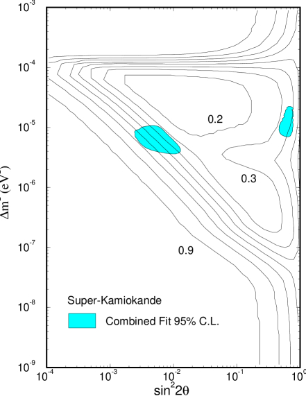
(a) Super-Kamiokande

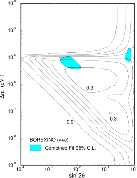
(b) BOREXINO

Fig. 20: The contours of the signal-to-SSM ratio for (a) Super-Kamiokande and (b) BOREXINO, along with the global MSW solutions (from present data) obtained in the Bahcall-Pinsonneault SSM. This is an updated result of Ref. [[31]].

3.6.4 Summary of MSW Signals

The parameter regions allowed by the combined observation are shown with the contours of the signal-to-SSM ratio in Fig. 20 for Super-Kamiokande and BOREXINO, assuming the Bahcall-Pinsonneault SSM. Given the high event rates in SNO, Super-Kamiokande, and BOREXINO, the accurate determination of the neutrino parameters should be possible.

The various characteristic signals from the global MSW solutions are summarized in Table 5. Also listed is the vacuum oscillation solution ($\Delta m^{2}\sim 8\times 10^{-11}\,\mbox{eV}\,^{2}$ and $\sin^{2}2\theta\sim 0.8$), which is allowed by the data, but requires a fine-tuning between the Sun-Earth distance and the neutrino parameters. It is stressed that the significance of establishing neutrino oscillations by the CC/NC measurement in SNO depends on the solar model. On the other hand, the effects of spectrum shape distortions, the day-night effect, and seasonal variations are free from solar model uncertainties and theoretically clean. An equivalent list for oscillations to sterile neutrinos are shown in Table 6.

Table 5: Characteristic signals expected in the global MSW solutions in flavor oscillations. The second large-angle solution is strongly disfavored by the data, and the solution only appears at 99% C.L. The vacuum oscillation solution is also listed. Whether SNO can definitively establish neutrino oscillations by the CC/NC measurement is solar model dependent.

	Oscillations to $\nu_{\mu,\tau}$
	Nonadiabatic	Large-Angle (I)	Large-Angle (II)	Vacuum
CC/NC	$\surd$	$\surd$	$\surd$	$\surd$
Spectrum Distortion	$\surd$			$\surd$
Day-Night Effect (8B)	?	$\surd$
Day-Night Effect (7Be)			$\surd$
Seasonal Variations				$\surd$

Table 6: Characteristic signals expected in the global MSW solutions for sterile neutrinos. The large-angle solutions (both (I) and (II)) and the vacuum solutions are strongly disfavored by the data and excluded for sterile neutrinos. The large-angle (I) solution is independently excluded by the big-bang nucleosynthesis constraint [61, 66].

	Oscillations to $\nu_{s}$
	Nonadiabatic	Large-Angle (I)	Large-Angle (II)	Vacuum
CC/NC
Spectrum Distortion	$\surd$			$\surd$
Day-Night Effect (8B)	?	$\surd$
Day-Night Effect (7Be)			$\surd$
Seasonal Variations				$\surd$

4 Summary and Wish List

4.1 Summary

Various theoretical models were confronted with the solar neutrino observations as possible solutions of the solar neutrino deficit. The astrophysical solutions are strongly disfavored by the data: (a) The SSM is excluded by the each of the experiments. (b) The model independent analysis concludes that the combined results from Homestake and Kamiokande exclude any astrophysical solutions. (c) Even if the Homestake data were discarded, we have no realistic solar model that simultaneously explains the Kamiokande and the gallium results within the experimental uncertainties.

The MSW mechanism, on the other hand, provides a complete description of the data, without discarding any of the observations. The parameter space allowed by the data is constrained to

Nonadiabatic: $$\;\Delta m^{2}\sim 10^{-5}\,\mbox{eV}\,^{2}\mbox{ and }\sin^{2}2\theta\sim 0.007$$ (11)

Large-angle: $$\;\Delta m^{2}\sim 10^{-5}\,\mbox{eV}\,^{2}\mbox{ and }\sin^{2}2\theta\sim 0.8.$$ (12)

There is a third allowed region for $\Delta m^{2}\sim 10^{-7}\,\mbox{eV}\,^{2}$ and $\sin^{2}2\theta\sim 0.8$, but only at 99% C.L. For oscillations to sterile neutrinos, the solution is allowed only in the nonadiabatic region.

The obtained parameters are sensitive to the solar model uncertainties. When nonstandard core temperatures are allowed, the data constrain $T_{C}=1.02\pm 0.02$ (1$\sigma$), consistent with the SSM. A wider MSW parameter space is possible in nonstandard solar models.

The predictions for the CC/NC ratio, spectrum distortions, and day-night effect in SNO and Super-Kamiokande were discussed in detail. It is stressed that the MSW prediction for the CC/NC ratio is solar model dependent, and a smaller ⁸B flux can make the difference between the MSW solutions and no-oscillations ambiguous.

4.2 Wish List

The solar neutrino experiments have provided us an opportunity for a better understanding of the Sun as well as a possible discovery of new neutrino physics. There will be more data soon, and much work is still needed involving experimentalists, astrophysicists, nuclear physicists, as well as particle physicists. The INT workshop allowed us to convene and discuss this inter-disciplinary topic, and, taking advantage of the opportunity, I will address my hopes from a particle physicist point of view:

From experimentalist friends:

• Uncertainty correlation matrix be published. In constraining the parameters in the MSW analysis, the energy spectrum and the time-divided data are very informative. From published papers, however, it is often not clear which of the systematic uncertainties are correlated among data points. In high-energy experiments such as in LEP, it is becoming more common to publish the correlation matrix, and I hope this trend will be followed in solar neutrino experiments.

From astrophysicist friends:

• The $S_{17}$ uncertainty be reevaluated. It is my belief that the current uncertainty obtained in Ref. [[15]] and used in the Bahcall-Pinsonneault model is underestimated. A larger uncertainty does not solve the solar neutrino problem; however, it does change the obtained MSW parameter space and affects the MSW predictions for the future experiments, especially the CC/NC ratio in SNO.

• A search for nonstandard solar models consistent with the Kamiokande and gallium data be pursued. There is no way one can reconcile the Homestake and Kamiokande data by astrophysical explanations. Even discarding the Homestake results entirely, we have no realistic solar model consistent both with the Kamiokande and gallium data, but more studies are needed. Especially, every nonstandard solar model should be confronted with the helioseismology data. If we cannot find a solar model consistent with the Kamiokande, gallium, and the helioseismology data after discarding the Homestake results, our motivation for new neutrino physics will be complete.

• Can the neutrino flux and the MSW parameters be constrained simultaneously? Once neutrino oscillations are established in the next generation experiments, the most significant task is to constrain the neutrino flux and the MSW parameters simultaneously from observations. This can be complicated since the MSW mechanism can distort the neutrino spectrum. Either simple relations among the fluxes (like the $T_{C}$ power laws) or Monte-Carlo models like the ones by Bahcall and Ulrich but with a wider range of solar models are needed. It would be ideal if the helioseismology data were incorporated in such an analysis.

Acknowledgments

This paper is based on the work done in collaboration with Sidney Bludman and Paul Langacker. I am grateful to P. Langacker for his careful reading of the manuscript and numerous valuable suggestions. I thank Institute for Nuclear Theory at the University of Washington for its hospitality and the Department of Energy for partial support during the time a part of this work was done. It is pleasure to thank the participants of the INT workshop for useful discussions; especially I have benefited from stimulating discussions with Anthony Baltz on the Earth effect. I also thank Eugene Beier for useful discussions. This work is supported by the Department of Energy Contract DE-AC02-76-ERO-3071.

References

- [1] J. N. Bahcall and M. H. Pinsonneault, Rev. Mod. Phys. 64, 885 (1992).
- [2] S. Turck-Chièze and I. Lopes, Astrophys. J. 408, 347 (1993). S. Turck-Chièze, S. Cahen, M. Cassé, and C. Doom, Astrophys. J. 335, 415 (1988).
- [3] R. Davis, Jr. et al., in Proceedings of the 21th International Cosmic Ray Conference, Vol. 12, edited by R. J. Protheroe (University of Adelaide Press, Adelaide, 1990), p. 143; R. Davis, Jr., in Frontiers of Neutrino Astrophysics, edited by Y. Suzuki and K. Nakamura (Universal Academy Press, Tokyo, 1993), P. 47.
- [4] K. Lande, private communications; B. Cleveland, private communications.
- [5] Kamiokande II Collaboration, K. S. Hirata et al., Phys. Rev. Lett. 65, 1297 (1990); 65, 1301(1990); 66, 9 (1991); Phys. Rev. D 44, 2241 (1991).
- [6] K. Nakamura, University of Tokyo Report No. ICRR-Report-312-94-7 (unpublished); Y. Suzuki, in Frontiers of Neutrino Astrophysics, edited by Y. Suzuki and K. Nakamura (Universal Academy Press, Tokyo, 1993) p. 61.
- [7] SAGE Collaboration, A. I. Abazov, et al., Phys. Rev. Lett. 67, 3332 (1991).
- [8] V. N. Gavrin, in Venice Workshop on Neutrino Telescopes, Venice, Italy, February, 1994.
- [9] GALLEX Collaboration, P. Anselmann et al., Phys. Lett. B 285, 376 (1992); 285, 390 (1992); 314, 445 (1993); GALLEX Report No. GX 44-1994 (submitted to Phys. Lett. B).
- [10] C. Charbonnel, these proceedings.
- [11] M. Pinsonneault, these proceedings.
- [12] P. Demarque, these proceedings.
- [13] S. A. Glasner, these proceedings.
- [14] M. Stix, these proceedings.
- [15] C. W. Johnson, E. Kolbe, S. E. Koonin, and K. Langanke, Astrophys. J. 392, 320 (1992).
- [16] K. Langanke, these proceedings.
- [17] R. W. Kavanagh, T. A. Tombrello, J. M. Mosher, and D. R. Goosman, Bull. Am. Phys. Soc., 14, 1209 (1969).
- [18] B. W. Filippone, A. J. Elwyn, C. N. Davids, and D. D. Koetke, Phys. Rev. Lett. 50, 412 (1983); Phys. Rev. C 28, 2222 (1983).
- [19] A. Dar and G. Shaviv, Technion preprint, 1994.
- [20] J. N. Bahcall et al., Los Alamos Bulletin Board Preprint No. astro-ph/9404002, 1994.
- [21] J. N. Bahcall, these proceedings.
- [22] P. Parker, these proceedings.
- [23] S. Bludman, D. Kennedy, and P. Langacker, Phys. Rev. D 45, 1810 (1992); Nucl. Phys. B 374, 373 (1992).
- [24] S. Bludman, N. Hata, D. Kennedy, and P. Langacker, Phys. Rev. D 47, 2220 (1993).
- [25] J. N. Bahcall and H. A. Bethe, Phys. Rev. D 47, 1298 (1993); Phys. Rev. Lett. 65, 2233 (1990); H. A. Bethe and J. N. Bahcall, Phys. Rev. D 44, 2962 (1991).
- [26] X. Shi and D. N. Schramm, Particle World 3, 109 (1994); D. N. Schramm and X. Shi, Fermilab Report No. FERMILAB-Pub-93/400-A, 1993 (to be published in Nucl. Phys. B, Proc. Suppl.).
- [27] S. Degl’Innocenti, these proceedings.
- [28] N. Hata, S. Bludman, and P. Langacker, Phys. Rev. D 49, 3622 (1994).
- [29] J. N. Bahcall and R. N. Ulrich, Rev. Mod. Phys. 60, 297 (1988).
- [30] J. N. Bahcall, Neutrino Astrophysics, (Cambridge University Press, Cambridge, England, 1989).
- [31] N. Hata and P. Langacker, University of Pennsylvania preprint UPR-0592T (1993, submitted to Phys. Rev. D.)
- [32] V. Castellani, S. Degl’Innocenti, and G. Fiorentini, Astron. Astrophys. 271, 601 (1993).
- [33] J. N. Bahcall, Phys. Rev. D 44, 1644 (1991).
- [34] D. Dearborn, private communications.
- [35] V. Castellani, S. Degl’Innocenti, and G. Fiorentini, Phys. Lett. B 303, 68 (1993).
- [36] J. Faulkner and R. L. Gilliland, Ap. J. 299, 994 (1985); R. L. Gilliland, J. Faulkner, W. H. Press, and D. N. Spergel, Ap. J. 306, 703 (1986).
- [37] A. De Rújula and S. L. Glashow, Report No. HUTP-92, CERN-TH 6608/92, 1992 (unpublished).
- [38] R. Davis, these proceedings.
- [39] R. Davis, in Progress in Particle and Nuclear Physics, Vol. 32, Erice, 1994.
- [40] R. Sienkiewicz, J. N. Bahcall, and B. Paczyński, Astrophys. J. 349, 641 (1990).
- [41] W. Merryfield, these proceedings.
- [42] See also X. Shi, D. N. Schramm, and D. S. P. Dearborn, Los Alamos Bulletin Board Preprint No. astro-ph/9404006, 1994.
- [43] D. Gough and J. Toomre, Annu. Rev. Astron. Astrophys. 29, 627 (1991); D. Gough, Phil. Trans. R. Soc. Lond. A 346, 37 (1994).
- [44] M. Gall-Mann, P. Ramond, and R. Slansky, in Supergravity, ed. F. van Nieuwenhuizen and D. Freedman (North Holland, Amsterdam 1979) p. 315; T. Yanagida, Prog. Theor. Phys. B135, 66 (1978).
- [45] L. Wolfenstein, Phys. Rev. D 17, 2369 (1978); 20, 2634 (1979); S. P. Mikheyev and A. Yu. Smirnov, Yad. Fiz. 42, 1441 (1985) [Sov. J. Nucl. Phys. 42, 913 (1985)]; Nuovo Cimento 9C, 17 (1986).
- [46] P. Langacker, in Proceedings of the 4th International Symposium on Neutrino Telescopes, Venice, Italy, 1992, edited by M. Bald-Ceolin, p. 73.
- [47] J. N. Bahcall and W. C. Haxton, Phys. Rev. D 40, 931 (1989).
- [48] X. Shi, D. N. Schramm, and J. N. Bahcall, Phys. Rev. Lett. 69, 717 (1992); X. Shi and D. N. Schramm, Phys. Lett. B 283, 305 (1992).
- [49] J. M. Gelb, W. Kwong, and S. P. Rosen, Phys. Rev. Lett. 69, 1864 (1992).
- [50] P. I. Krastev and S. T. Petcov, Phys. Lett. B 299, 99 (1993).
- [51] L. Krauss, E. Gates, and M. White, Phys. Lett. B 299, 94 (1993).
- [52] G. L. Fogli, E. Lisi, and D. Montanino, Phys. Rev. D 49, 3626 (1994).
- [53] G. Fiorentini et al., INFN Report No. INFNFE-10-93, 1993 (submitted to Phys. Rev. D).
- [54] N. Hata and P. Langacker, Phys. Rev. D 48, 2937 (1993).
- [55] A. J. Baltz and J. Weneser, Phys. Rev. D 35, 528 (1987); 37, 3364, (1988); E. D. Carlson, Phys. Rev. D 34, 1454 (1986); J. Bouchez, M. Cribier, W. Hampel, J. Rich, M. Spiro, and D. Vignaud, Z. Phys. C 32, 499 (1986); M. Cribier, W. Hampel, J. Rich, and D. Vignaud, Phys. Lett. B 182, 89 (1986); S. Hiroi, H. Sakuma, T. Yanagida, and M. Yoshimura, Prog. Theor. Phys. 78, 1428 (1987); A. Dar, A. Mann, Y. Melina, and D. Zajfman, Phys. Rev. D 35 3607, (1987); P. I. Krastev and S. T. Petcov, Phys. Lett. B 205, 84 (1988); R. S. Raghavan et al., Phys. Rev. D 44 3786, (1991); J. M. LoSecco, Phys. Rev. D 47, 2032 (1993); V. Barger, K. Whisnant, S. Pakvasa, and R. J. N. Phillips, Phys. Rev. D 22, 2718 (1980).
- [56] F. D. Stacy, Physics of the Earth, 2nd ed. (Wiley, New York, 1985), p. 171; T. H. Jordan and D. L. Anderson, Geophys. J. R. Astron. Soc. 36, 411 (1974).
- [57] S. T. Petcov, Phys. Lett. B 200, 373 (1988); Nucl. Phys. B (Proc. Suppl.) 13, 527 (1990).
- [58] T. K. Kuo and J. Pantaleone, Rev. Mod. Phys. 61, 937 (1989).
- [59] S. J. Parke, Phys. Rev. Lett. 57, 1275 (1986).
- [60] P. Pizzochero, Phys. Rev. D 36, 2293 (1987).
- [61] P. Langacker, University of Pennsylvania Report No., UPR 0401T (1989); R. Barbieri and A. Dolgov, Nucl. Phys. B 349, 743 (1991); K. Enqvist, K. Kainulainen, and J. Maalampi, Phys. Lett. B 249, 531 (1990); M. J. Thomson and B. H. J. McKellar, Phys. Lett. B 259, 113 (1991); V. Barger et al., Phys. Rev. D 43, 1759 (1991); P. Langacker and J. Liu, Phys. Rev. D 46, 4140 (1992). X. Shi, D. Schramm, and B. Fields, Phys. Rev. D 48, 2563 (1993).
- [62] See, for example, E. Beier et al., Phys. Lett. B283, 446 (1992), and references therein.
- [63] G. Smoot et al., Astrophys. J. 396, L1 (1992); E.Ł. Wright et al., Astrophys. J. 396, L13 (1992); R. Schaefer and Q. Shafi, Bartol Research Institute Report No. BA-93-52; Nature 359, 199 (1992); A. Klypin, J. Holtzman, J. Primack, and E. Regos, University of California (Santa Cruz) Report No. SCIPP-92-52; R. L. Davis et al., Phys. Rev. Lett. 69, 1856 (1992).
- [64] N. Hata, University of Pennsylvania Report No. UPR-0605T (unpublished), and references therein.
- [65] G. Bernardi, in XXIV International Conference on High Energy Physics edited by R. Kotthaus and J. Kühn (Springer, Berlin, 1989) p. 1076.
- [66] X. Shi, D. Schramm, and B. Fields, in Ref. [[61]].
- [67] M. Cvetič and P. Langacker, Phys. Rev. D 46, R2759 (1992).
- [68] G. T. Ewan et al. “Sudbury Neutrino Observatory Proposal”, Report No. SNO-87-12, 1987 (unpublished); “Scientific and Technical Description of the Mark II SNO Detector”, edited by E. W. Beier and D. Sinclair, Report No. SNO-89-15, 1989 (unpublished).
- [69] Y. Totsuka, University of Tokyo (ICRR) Report No. ICCR-Report-227-90-20, 1990 (unpublished).
- [70] “BOREXINO at Gran Sasso — proposal for a real time detector for low energy solar neutrinos”, Vol. 1, edited by G. Bellini, M. Campanella, D. Giugni, and R. Raghavan (1991).
- [71] C. Rubbia, Report No. CERN-PPE/93-08, 1993 (unpublished).
- [72] S. Nozawa, private communications.
- [73] M. Doi and K. Kubodera, Phys. Rev. C 45, 1988 (1992); S. Ying, W. Haxton, and E. Henley Phys. Rev. C 45, 1982 (1992); K. Kubodera and S. Nozawa, University of South Carolina Report No. USC(NT)-93-6 (unpublished) and references therein.
- [74] A. Baltz and J. Weneser, work in progress; A. Baltz, talk given at Institute of Nuclear Theory, University of Washington, Seattle, March 28, 1994.