Preprint numbers: ADP-93-225/T142

ANL-PHY-7668-TH-93

DYSON-SCHWINGER EQUATIONS AND THEIR

APPLICATION TO HADRONIC PHYSICS

Craig D. Roberts and Anthony G. Williams

Physics Division, Argonne National Laboratory, Argonne, IL 60439-4843, USA

Department of Physics and Mathematical Physics, University of Adelaide,

S.A. 5005, Australia

Department of Physics and the Supercomputer Computations Research Institute,

Florida State University, Tallahassee, FL 32306, U.S.A.

e-mail: cdroberts@anl.gov, awilliam@physics.adelaide.edu.au

ABSTRACT

We review the current status of nonperturbative studies of gauge field theory using the Dyson-Schwinger equation formalism and its application to hadronic physics. We begin with an introduction to the formalism and a discussion of renormalisation in this approach. We then review the current status of studies of Abelian gauge theories [e.g., strong coupling quantum electrodynamics] before turning our attention to the non-Abelian gauge theory of the strong interaction, quantum chromodynamics. We discuss confinement, dynamical chiral symmetry breaking and the application and contribution of these techniques to our understanding of the strong interactions.

KEYWORDS

confinement of quarks and gluons; dynamical chiral symmetry breaking; Dyson-Schwinger equations; hadrons; quantum electrodynamics; quantum chromodynamics.

To appear in Progress in Particle and Nuclear Physics

1 Introduction

As computer technology continues to improve, lattice gauge theory [LGT] will become an increasingly useful means of studying hadronic physics through investigations of discretised quantum chromodynamics [QCD]. [For a recent review of LGT with numerous references see Rothe (1992).] However, it is equally important to develop other complementary nonperturbative methods based on continuum descriptions. In particular, with the advent of new accelerators such as CEBAF and RHIC, there is a need for the development of approximation techniques and models which bridge the gap between short-distance, perturbative QCD and the extensive amount of low- and intermediate-energy phenomenology in a single covariant framework. Cross-fertilisation between LGT studies and continuum techniques provides a particularly useful means of developing a detailed understanding of nonperturbative QCD.

One such continuum approach is based on the infinite tower of Dyson-Schwinger equations [DSEs]. The DSEs are coupled integral equations which relate the Green’s functions of a field theory to each other. Solving these equations provides a solution of the theory; a field theory being completely defined when all of its $n$-point Green’s functions are known. The DSEs include, for example, the Bethe-Salpeter equation [BSE] which is needed for the description of relativistic two-body scattering and bound states. Quantitative studies of a field theory must be based on one [or more] systematic approximation schemes: for example, perturbation theory for weak coupling; lattice studies using increasing numbers of sites and $\beta$-values in order to represent a larger volume of the spacetime-continuum; large $N$ expansions for $SU(N)$ gauge theories; $\hbar$ expansions for semiclassical approximations; etc. For studies based on DSEs it is unavoidable that the infinite tower of coupled equations must be truncated at some point. This means that the tower of equations must be limited to some $n$, where $n$ is the maximum number of legs on any Green’s function included in the self-consistent solution of the equations. Because of the complex issues involved and the computational effort required, current efforts are necessarily modest; for example, we know of no attempts as yet to study coupled DSEs for $n>3$. The penalty incurred by truncation is the need to employ an Ansatz for the omitted function(s). However, much can be achieved by exploiting the need to maintain certain properties of the theory, including the various global and local symmetries, multiplicative renormalisability, analyticity, known perturbative behaviour in the weak coupling limit, etc. These can provide stringent constraints on the Ansätze. In addition, there is the hope that future lattice gauge theory simulations will be able to provide additional insight into the form of these higher $n$-point functions.

In Sec. 2 we introduce the DSE formalism, beginning with a discussion of Abelian gauge theories [quantum electrodynamics in three- and four-dimensions, QED₃ and QED₄ ] and then extend this discussion to QCD. In Secs. 3 and 4 we review in some detail the current status of DSE-based studies of QED₃ and QED₄ with particular emphasis on gauge covariance and multiplicative renormalisability. Such studies are extremely useful as a guide to the more complicated case of QCD. We devote Sec. 5 to a study of the gauge boson sector of QCD and focus on studies of the infrared behaviour of the gluon propagator, since this is thought to be crucial to confinement in QCD. In Sec. 6 we examine the quark sector of QCD, discussing the crucial issues of dynamical chiral symmetry breaking [DCSB] and quark confinement. In Sec. 7 we review applications of the ideas discussed in the preceding sections to studies of hadronic structure. Finally, in Sec. 8, we summarise and discuss possible future extensions of these studies.

2 Dyson-Schwinger Equation Formalism

It has been known for quite some time that, from the field equations of a quantum field theory, one can derive a system of coupled integral equations relating the Green’s functions for the theory to each other (Dyson, 1949; Schwinger, 1951). This infinite tower of equations is sometimes referred to as the complex of Dyson-Schwinger equations. An introduction to the formal details of DSEs, including their derivation etc., can be found in a number of text books; Bjorken and Drell (1965, pp. 283-376) and Itzykson and Zuber (1980, pp. 475-481) are two examples. For completeness we will summarise those aspects of the formalism which are relevant to the gauge field theories of quantum electrodynamics [QED] and quantum chromodynamics [QCD]. These are the areas where the DSE approach to the solution of a quantum field theory [QFT] has been applied most widely. Our exposition employs the functional integral formulation of these field theories; useful introductions to which can be found in Itzykson and Zuber (1980, pp. 425-474) and Rivers (1987). The separate but related question of whether the functional integral formulation of these field theories can be rigorously defined is as yet unresolved. A discussion of this problem can be found, for example, in Seiler (1982). The Euclidean-space, discretised, lattice theory is well-defined, but there the question is simply deferred and becomes a question of rigorously establishing the existence of the continuum limit. This limit is a critical point of the lattice theory, since, in units of the lattice spacing, physical correlation lengths must diverge.

2.1 Quantum Electrodynamics [QED]

In the following we will discuss quantum electrodynamics in $D=2$ and $D=3$ space dimensions, referred to as QED₃ and QED₄ respectively. We denote the number of space-time dimensions as ${\rm d}=D+1$ and write the action for QED_d in Minkowski metric, with signature $g_{00}=1$ and $g_{ii}=-1$ for $i=1\ldots D$:

$$S[\mbox{$\overline{\psi}$},\psi,A_{\mu}]=\int\,d^{\rm d}x\;\left[\,\sum_{f=1}^{N_{f}}\,\mbox{$\overline{\psi}$}^{f}\left(i\mbox{$\not\!\partial$}-m_{0}^{f}+e_{0}^{f}\mbox{$\not\!\!A$}\right)\psi^{f}-\frac{1}{4}F_{\mu\nu}F^{\mu\nu}\right]~{}.$$ (2.1)

[We have set $\hbar=1=c$.] In Eq. (2.1) the superscript $f$ is a flavour label; $f=1\ldots N_{f}$ for a theory with $N_{f}$ distinct types or flavours of electrically active fermions, each represented by the field $\psi^{f}(x)$; $m_{0}^{f}$ and $e_{0}^{f}$ are, respectively, the bare mass and charge of each of these fermions; $A_{\mu}(x)$ is the gauge-boson [photon] field; and

$$F_{\mu\nu}=\partial_{\mu}A_{\nu}-\partial_{\nu}A_{\mu}$$ (2.2)

is the Abelian gauge-boson field strength tensor. We use standard notation and conventions, where $\mbox{$\not\!\!A$}=A_{\mu}\gamma^{\mu}=g^{\mu\nu}A_{\mu}\gamma_{\nu}$, $\{\gamma^{\mu},\gamma^{\nu}\}=2g^{\mu\nu}$, $\gamma_{5}=i\gamma^{0}\gamma^{1}\gamma^{2}\gamma^{3}$, etc. Note that for an electron we would have for the [physical] charge $e^{f}=-e$, where by definition $e=|e|$ is the magnitude of the electron charge.

The quantum field theory associated with Eq. (2.1) is defined by the generating functional

$${\cal Z}[\mbox{$\overline{\eta}$},\eta,J_{\mu}]=\int\,d\mu(\mbox{$\overline{\psi}$},\psi,A)\,\exp\left(iS[\mbox{$\overline{\psi}$},\psi,A_{\mu}]+i\int\,d^{\rm d}x\;\left[\,\sum_{f}\left(\mbox{$\overline{\psi}$}^{f}\eta^{f}+\mbox{$\overline{\eta}$}^{f}\psi^{f}\right)+A_{\mu}J^{\mu}\right]\right)$$ (2.3)

where $\mbox{$\overline{\eta}$}^{f}$, $\eta^{f}$ and $J_{\mu}$ are, respectively, source fields for the fermion, antifermion and gauge boson and where we have defined

$$d\mu(\mbox{$\overline{\psi}$},\psi,A)=\prod_{f}\,{\cal D}\mbox{$\overline{\psi}$}^{f}{\cal D}\psi^{f}\prod_{\mu}\,{\cal D}A_{\mu}~{}.$$ (2.4)

[A constant normalisation factor is understood which ensures that ${\cal Z}[0,0,0]=1$.] This generating functional is the field theoretic analogue of the partition function of a statistical mechanical system and serves the same purpose; i.e., all the physical quantities of the theory can be obtained from ${\cal Z}[\mbox{$\overline{\eta}$},\eta,J_{\mu}]$.

Operationally, the integral in Eq. (2.3) represents “an integral over all possible values of each of the fields at all spacetime points”. Detailed discussions of the functional integral can be found in Rivers (1987), Pascual and Tarrach (1984, pp. 198-226) and Seiler (1982). For our purposes, however, we may proceed upon noting that the fermion fields $\{\mbox{$\overline{\psi}$},\psi\}$ and their sources $\{\mbox{$\overline{\eta}$},\eta\}$ are elements of a Grassmann algebra with involution which entails that all of these fields anticommute with each other [this ensures that Fermi-statistics are obeyed by the fermion fields]; and that $A_{\mu}$ and its source $J_{\mu}$ are c-number fields.

In order to complete the operational definition of QED_d we note that the action in Eq. (2.1) is invariant under the local Abelian gauge transformation

$$\psi(x)\rightarrow\;^{\lambda}\!\psi(x) = {\rm e}^{-ie_{0}\lambda(x)}\psi(x)\;\;,\;\;\mbox{$\overline{\psi}$}(x)\rightarrow\;^{\lambda}\!\,\mbox{$\overline{\psi}$}(x)={\rm e}^{ie_{0}\lambda(x)}\mbox{$\overline{\psi}$}(x)\;,$$

$$A_{\mu}(x)\rightarrow\;^{\lambda}\!A_{\mu}(x) = A_{\mu}(x)-\partial_{\mu}\lambda(x)$$ (2.5)

where $\lambda(x)$ is an arbitrary scalar function and, for now, we have suppressed the flavor indices. This entails that the generating functional as it has been defined so far is meaningless [even assuming that our above caveats have been properly taken into account]. This is because gauge invariance ensures that for any field configuration, {$\mbox{$\overline{\psi}$}(x),\psi(x),A_{\mu}(x)$}, there are [uncountably] many related configurations, {${}^{\lambda}\!\mbox{$\overline{\psi}$}(x),^{\lambda}\!\psi(x),^{\lambda}\!A_{\mu}(x)$}, which have the same action; i.e.,

$$S[\mbox{$\overline{\psi}$},\psi,A_{\mu}]=S[^{\lambda}\!\mbox{$\overline{\psi}$},^{\lambda}\!\psi,^{\lambda}\!A_{\mu}]\;.$$ (2.6)

The Grassmann integration over $\overline{\psi}$ and $\psi$ gives the same result independent of $\lambda(x)$ since the corresponding Grassmannian Jacobian for this transformation is unity. Hence there is an overall volume divergence in the functional integration over the gauge field $A_{\mu}$ in Eq. (2.3). This is analogous to the divergence one obtains in the spacetime integral of a translationally invariant function. The proper definition of the measure in Eq. (2.4) must ensure that the gauge field integration extends only over gauge-inequivalent configurations (Bailin and Love, 1986, pp. 116-119).

This problem can be resolved via the introduction of the Faddeev-Popov determinant (Popov, 1983). [Historically, this first arose in connection with the correct quantisation of non-Abelian gauge theories (Faddeev and Popov, 1967).] The net effect of this procedure in QED_d is simply to introduce a gauge fixing term into the action of Eq. (2.3) (Rivers, 1987, pp. 182-185). A common choice for this is the covariant gauge fixing term, which we use here, and which gives

$$S[\mbox{$\overline{\psi}$},\psi,A_{\mu}]\rightarrow S_{\xi}[\mbox{$\overline{\psi}$},\psi,A_{\mu}]=S[\mbox{$\overline{\psi}$},\psi,A_{\mu}]-\frac{1}{2\xi_{0}}\int\,d^{\rm d}x\,\left(\partial_{\mu}A^{\mu}\right)^{2}~{},$$ (2.7)

where $\xi_{0}$ is the bare gauge fixing parameter. It should be noted that the difficulty with gauge fixing involving Gribov ambiguities does not appear in Abelian gauge theories, [unless one adopts unusual nonlinear gauge fixing prescriptions]. It can be shown that physical observables are independent of the [renormalised] gauge parameter, $\xi$, and, in fact, that they are independent of the actual form of the gauge fixing term (Bailin and Love, 1986, pp. 330-334 and references therein). The unrenormalised quantum field theory of electrodynamics is then defined by Eq. (2.3) with the action $S_{\xi}$ of Eq. (2.7) and we may now proceed to obtain the unrenormalised DSEs.

Unrenormalised Dyson-Schwinger equation for the Photon Polarisation Tensor.       The example of the derivation of the DSE for the photon polarisation tensor in QED₄ is given in Itzykson and Zuber (1980, pp. 476-477) and we summarise these arguments here to illustrate the technique and to emphasise the fact that the DSEs are simply the Euler-Lagrange equations of quantum field theory. It should also be noted that independent of this functional analysis one can directly obtain these equations by simply decomposing the infinite sums of Feynman diagrams for Green’s functions in terms of other proper and full Green’s functions. This Feynman diagram approach is explained in some detail in Bjorken and Drell (1965, pp. 283-376).

Consider the generating functional of Eq. (2.3) with the action of Eq. (2.7). It can be shown [e.g., Itzykson and Zuber (1980, pp. 211-212)] that the generating functional of connected Green’s functions, ${\cal G}[\mbox{$\overline{\eta}$},\eta,J_{\mu}]$, is defined via

$${\cal Z}[\mbox{$\overline{\eta}$},\eta,J_{\mu}]=\exp\left({\cal G}[\mbox{$\overline{\eta}$},\eta,J_{\mu}]\right)~{}.$$ (2.8)

In order to obtain the DSEs one must simply note that, in analogy with the case of standard calculus, the functional integral of a total functional derivative is zero given appropriate boundary conditions, [see, e.g., Collins (1984, pp. 13-15)]. Hence, for example,

$$0 = \int d\mu(\mbox{$\overline{\psi}$},\psi,A)\,\frac{\delta}{\delta A_{\mu}(x)}\exp\left\{i\left(S_{\xi}[\mbox{$\overline{\psi}$},\psi,A_{\mu}]+\int\,d^{\rm d}x\;\left[\mbox{$\overline{\psi}$}^{f}\eta^{f}+\mbox{$\overline{\eta}$}^{f}\psi^{f}+A_{\mu}J^{\mu}\right]\right)\right\}$$ (2.9)

$$= \int d\mu(\mbox{$\overline{\psi}$},\psi,A)\,\left\{\frac{\delta S_{\xi}}{\delta A_{\mu}(x)}+J_{\mu}(x)\right\}\exp\left\{i\left(S_{\xi}[\mbox{$\overline{\psi}$},\psi,A_{\mu}]+\int\,d^{\rm d}x\;\left[\mbox{$\overline{\psi}$}^{f}\eta^{f}+\mbox{$\overline{\eta}$}^{f}\psi^{f}+A_{\mu}J^{\mu}\right]\right)\right\}$$

$$= \left\{\frac{\delta S_{\xi}}{\delta A_{\mu}(x)}\left[\frac{\delta}{i\delta J},\frac{\delta}{i\delta\mbox{$\overline{\eta}$}},-\frac{\delta}{i\delta\eta}\right]+J_{\mu}(x)\right\}{\cal Z}[\mbox{$\overline{\eta}$},\eta,J_{\mu}]~{}.$$

Differentiating Eq. (2.7) immediately gives

$$\frac{\delta S_{\xi}}{\delta A_{\mu}(x)}=\left[\partial_{\rho}\partial^{\rho}g_{\mu\nu}-\left(1-\frac{1}{\xi_{0}}\right)\partial_{\mu}\partial_{\nu}\right]A^{\nu}+\sum_{f}e_{0}^{f}\,\mbox{$\overline{\psi}$}^{f}\gamma_{\mu}\psi^{f}$$ (2.10)

from which it follows that after dividing through by ${\cal Z}$ we can write Eq. (2.9) as

$$\left[\partial_{\rho}\partial^{\rho}g_{\mu\nu}-\left(1-\frac{1}{\xi_{0}}\right)\partial_{\mu}\partial_{\nu}\right]\frac{\delta{\cal G}}{i\delta J_{\nu}(x)}+\sum_{f}e_{0}^{f}\,\left(\frac{\delta{\cal G}}{\delta\eta^{f}(x)}\gamma_{\mu}\frac{\delta{\cal G}}{\delta\mbox{$\overline{\eta}$}^{f}(x)}+\frac{\delta}{\delta\eta^{f}(x)}\left[\gamma_{\mu}\frac{\delta{\cal G}}{\delta\mbox{$\overline{\eta}$}^{f}(x)}\right]\right)=-J_{\mu}(x)~{}.$$ (2.11)

Equation. (2.11) represents a compact form of the nonperturbative equivalent of Maxwell’s equations. To illustrate this we use it to obtain an expression for the photon vacuum polarisation. We can now perform a Legendre transformation and introduce the generating functional for the connected, one-particle irreducible [1-PI] Green’s functions, $\Gamma[\mbox{$\overline{\psi}$},\psi,A_{\mu}]$:

$${\cal G}[\mbox{$\overline{\eta}$},\eta,J_{\mu}]\equiv i\Gamma[\mbox{$\overline{\psi}$},\psi,A_{\mu}]+i\int\,d^{\rm d}x\;\left[\mbox{$\overline{\psi}$}^{f}\eta^{f}+\mbox{$\overline{\eta}$}^{f}\psi^{f}+A_{\mu}J^{\mu}\right]~{}.$$ (2.12)

An explanation of the fact that $\Gamma[\mbox{$\overline{\psi}$},\psi,A_{\mu}]$ generates the 1-PI Green’s functions is given in Itzykson and Zuber (1980, pp. 289-294). The 1-PI Green’s functions are also frequently referred to as the proper Green’s functions. It follows from the rules of Grassmannian integration that ${\cal Z}[\mbox{$\overline{\eta}$},\eta,J_{\mu}]$ and hence ${\cal G}[\mbox{$\overline{\eta}$},\eta,J_{\mu}]$ depend only on powers of pairs of $\overline{\eta}$ and $\eta$, which implies that setting $\mbox{$\overline{\eta}$}=\eta=0$ after differentiating ${\cal G}$ [or ${\cal Z}$] will only give a nonzero result for equal numbers of $\overline{\eta}$ and $\eta$ derivatives. Similarly, in the absence of fermion derivatives it can be seen that only even numbers of derivatives of ${\cal Z}$ and ${\cal G}$ with respect to $J$ survive when we set $J=0$, which immediately leads to Furry’s theorem for QED, [see, e.g., Itzykson and Zuber (1980, pg. 276)]. Throughout this work we diagrammatically represent proper Green’s functions by unfilled circles and full [connected] Green’s functions by shaded circles. See, e.g., Fig. 2.1, where the use of the proper electron-photon vertex, $\Gamma^{f\mu}$, is necessary to avoid the double-counting of Feynman diagrams using the arguments of Bjorken and Drell op cit. From Eq. (2.12) the following relations immediately follow:

$$\begin{array}[]{ccc}A_{\mu}(x)=\displaystyle\frac{\delta{\cal G}}{i\delta J^{\mu}(x)},&\psi^{f}(x)=\displaystyle\frac{\delta{\cal G}}{i\delta\mbox{$\overline{\eta}$}^{f}(x)},&\mbox{$\overline{\psi}$}^{f}(x)=\displaystyle-\,\frac{\delta{\cal G}}{i\delta\eta^{f}(x)},\\ J_{\mu}(x)=\displaystyle-\,\frac{\delta\Gamma}{\delta A^{\mu}(x)},&\eta^{f}(x)=\displaystyle-\,\frac{\delta\Gamma}{\delta\mbox{$\overline{\psi}$}^{f}(x)},&\mbox{$\overline{\eta}$}^{f}(x)=\displaystyle\frac{\delta\Gamma}{\delta\psi^{f}(x)}~{}.\end{array}$$ (2.13)

From Eq. (2.13) we see that we now have expressions for $\mbox{$\overline{\psi}$},\psi$, and $A_{\mu}$ in terms of $\mbox{$\overline{\eta}$},\eta$, and $J_{\mu}$ and vice versa; i.e., $\mbox{$\overline{\psi}$}^{f}_{\alpha}(x)=\mbox{$\overline{\psi}$}^{f}_{\alpha}[\mbox{$\overline{\eta}$},\eta,J_{\mu}(x)]=i\delta{\cal G}[\mbox{$\overline{\eta}$},\eta,J_{\mu}]/\delta\eta^{f}_{\alpha}(x)$ with the spinor index $\alpha$ now explicitly shown. It is now easy to see that setting $\mbox{$\overline{\psi}$}=\psi=0$ after differentiating $\Gamma$ gives a nonzero result only when there are equal numbers of $\overline{\psi}$ and $\psi$ derivatives in analogy to the case for ${\cal G}$. Using Eq. (2.13) and the fact that $\delta\mbox{$\overline{\psi}$}^{f}_{\alpha}/\delta\mbox{$\overline{\psi}$}^{g}_{\beta}=\delta_{\alpha\beta}\delta_{fg}\delta^{\rm d}(x-y)$ we find that

$$\left.i\int d^{\rm d}z\,\frac{\delta^{2}{\cal G}}{\delta\eta_{\alpha}^{f}(x)\mbox{$\overline{\eta}$}_{\gamma}^{h}(z)}\,\frac{\delta^{2}\Gamma}{\delta\psi_{\gamma}^{h}(z)\mbox{$\overline{\psi}$}_{\beta}^{g}(y)}\right|_{\begin{array}[]{c}\eta=\mbox{$\overline{\eta}$}=0\\ \psi=\overline{\psi}=0\end{array}}=\delta_{rs}\delta_{fg}\delta^{\rm d}(x-y)\;.$$ (2.14)

Hence it follows that, when the fermion sources ($\mbox{$\overline{\eta}$},\eta$) vanish, Eq. (2.11) can be written as

$$\left.\frac{\delta\Gamma}{\delta A^{\mu}(x)}\right|_{\psi=\overline{\psi}=0}=\left[\partial_{\rho}\partial^{\rho}g_{\mu\nu}-\left(1-\frac{1}{\xi_{0}}\right)\partial_{\mu}\partial_{\nu}\right]A^{\nu}(x)-i\sum_{f}e_{0}^{f}{\rm tr}\left[\gamma_{\mu}S^{f}(x,x,[A_{\mu}])\right]\;,$$ (2.15)

where we have made the identification

$$S^{f}(x,y,[A_{\mu}])=\left(\left.\frac{\delta^{2}\Gamma}{\delta\mbox{$\overline{\psi}$}^{f}(x)\delta\psi^{f}(y)}\right|_{\psi=\overline{\psi}=0}\right)^{-1}\;,$$ (2.16)

which is the propagator of the fermion of flavour $f$ in an external electromagnetic field $A_{\mu}$. This identification follows from Eq. (2.14) and the fact that the second derivative of ${\cal G}$ is the full 2-point fermion Green’s function; i.e., the fermion propagator in the presence of a background field, $S^{f}(x,y,[A_{\mu}])$. Clearly, the full fermion Green’s function $S^{f}(x,y)$ follows from setting $A_{\mu}=0$ in Eq. (2.16).

To obtain the DSE for the photon polarisation tensor it remains only to act with $\delta/\delta A_{\nu}(y)$ on Eq. (2.15) and set $J_{\mu}(x)=0$. It can be shown that

$$\left.e_{0}^{f}\,\Gamma^{f}_{\mu}(x;y,z)=\frac{\delta}{\delta A^{\mu}(x)}\frac{\delta^{2}\Gamma}{\delta\mbox{$\overline{\psi}$}^{f}(y)\delta\psi^{f}(z)}\right|_{0=A_{\mu}=\psi=\overline{\psi}}~{},$$ (2.17)

is the proper [i.e., 1-PI] fermion–gauge–boson vertex [not to be confused with the generating functional $\Gamma$]. Similarly to the fermion case it can be shown that the second derivative of $\Gamma$ with respect to $A$ gives the inverse photon propagator, $(D^{-1})^{\mu\nu}(x,y)$. Thus from Eq. (2.15) we obtain the DSE for the inverse photon propagator

$$(D^{-1})^{\mu\nu}(x,y)=\left.\frac{\delta^{2}\Gamma}{\delta A^{\mu}(x)\delta A^{\nu}(y)}\right|_{A_{\mu}=\psi=\overline{\psi}=0}=\left[\partial_{\rho}\partial^{\rho}g_{\mu\nu}-\left(1-\frac{1}{\xi_{0}}\right)\partial_{\mu}\partial_{\nu}\right]\delta^{\rm d}(x-y)+\Pi_{\mu\nu}(x,y)$$ (2.18)

where we have defined the photon polarisation tensor, $\Pi_{\mu\nu}$:

$$\Pi_{\mu\nu}(x,y)=i\sum_{f}(e_{0}^{f})^{2}\int\,d^{\rm d}z_{1}\,d^{\rm d}z_{2}\,{\rm tr}\left[\gamma_{\mu}S^{f}(x,z_{1})\Gamma^{f}_{\nu}(y;z_{1},z_{2})S^{f}(z_{2},x)\right]\;.$$ (2.19)

Using translational invariance we can write the photon propagator in momentum space as

$$D^{\mu\nu}(q)=\frac{-g^{\mu\nu}+(q^{\mu}q^{\nu}/(q^{2}+i\epsilon))}{q^{2}+i\epsilon}\frac{1}{1+\Pi(q^{2})}-\xi_{0}\frac{q^{\mu}q^{\nu}}{(q^{2}+i\epsilon)^{2}}\;,$$ (2.20)

where we have made use of the Ward-Takahashi identity [WTI] for the photon propagator,

$$q_{\mu}\Pi^{\mu\nu}(q)=0~{},$$ (2.21)

to define $\Pi(q^{2})$ by $\Pi^{\mu\nu}(q)\equiv(-g^{\mu\nu}q^{2}+q^{\mu}q^{\nu})\Pi(q^{2})$. Note that $\Pi(q^{2})$ is independent of the gauge parameter $\xi_{0}$ in QED as a result of current conservation. A discussion of WTIs is given, for example, in Itzykson and Zuber (1980, pp. 407-411) and in Bjorken and Drell (1965, pp. 299-303). There is a whole family of such identities, which follow from the fact that gauge invariance leads to the conservation of the electromagnetic [e.m.] current. Because renormalisation does not affect e.m. current conservation the WTIs also apply to the renormalised Green’s functions of the theory provided that the regularisation of infinities is performed in a gauge-invariant way. That $\Pi^{\mu\nu}$ is transverse leads to the fact that the photon remains massless, [see, e.g., Itzykson and Zuber (1980, pp. 318-329]. The cases $\xi_{0}=0$ and 1 are referred to as Landau and Feynman gauges respectively [and similarly for $\xi$ after renormalisation]. The normalisations in these equations are such that at lowest order in perturbation theory we have $\Pi=0$, as well as

$$\Gamma^{f}_{\nu}(y;z_{1},z_{2})=\gamma_{\nu}\,\delta^{\rm d}(y-z_{1})\,\delta^{\rm d}(y-z_{2})\;\;\;\;{\rm and}\;\;\;\;(i\not\!\partial-m_{0}^{f})\,S^{f}(x,y)=\delta^{\rm d}(x-y)~{}.$$ (2.22)

It should be noted that, once $e_{0}^{f}$ is factored out, there is no explicit flavour dependence in the proper vertex since the same sum of Feynman diagrams will contribute in each case. We will later see that once we define the renormalised charge through appropriate boundary conditions a flavour-dependence still arises for nondegenerate fermion masses.

We have seen that second derivatives of the generating functional, $\Gamma[\mbox{$\overline{\psi}$},\psi,A_{\mu}]$, give the inverse fermion and photon propagators and that the third derivative gave the proper photon-fermion vertex. In general, all derivatives of the generating functional, $\Gamma[\mbox{$\overline{\psi}$},\psi,A_{\mu}]$, higher than two produce the corresponding proper Green’s functions, where the number and type of derivatives give the number and type of proper Green’s function legs.

The DSE for the photon propagator is represented diagrammatically in Fig. 2.1. Part a) of the figure represents Eq. (2.19) for the photon polarisation tensor and part b) shows the photon propagator, $D^{\mu\nu}(x,y)$, defined in terms of $\Pi^{\mu\nu}(x,y)$ and the bare photon propagator, $D_{0}^{\mu\nu}(x,y)$ [given by Eq. (2.20) with $\Pi=0$] and corresponds to the inverse of Eq. (2.18).

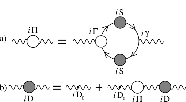
Fig. 2.1: The Dyson-Schwinger equation for the photon propagator.

The momentum-space representation of the DSEs is readily obtained by either Fourier transforming the coordinate-space form or, more readily, by using the standard rules for Feynman diagrams based on the lowest-order perturbative contribution to the nonperturbative quantities. For example, for the photon polarisation tensor we obtain

$$i\Pi_{\mu\nu}(q)=(-1)\sum_{f}(e_{0}^{f})^{2}\int\frac{d^{\rm d}\ell}{(2\pi)^{\rm d}}{\rm tr}[(i\gamma_{\mu})(iS^{f}(\ell))(i\Gamma^{f}(\ell,\ell+q))(iS^{f}(\ell+q))]\;,$$ (2.23)

where the factor of $(-1)$ arises from the fermion loop in the usual way. We have elected to not explicitly show such factors of $(-1)$ in the diagrammatic representation. In momentum space, Fig. 2.1b) corresponds to $iD^{\mu\nu}(q)=iD_{0}^{\mu\tau}(q)[\delta^{\nu}_{\tau}+i\Pi_{\tau\rho}(q)iD^{\rho\nu}(q)]$, which can be obtained from the Fourier transform of Eq. (2.20). Throughout this work we use figures like Fig. 2.1 and the associated notation so that the momentum space equations are easily written down by inspection.

Unrenormalised Dyson-Schwinger equation for the Fermion Self Energy.       Following a procedure similar to that above (Itzykson and Zuber, 1980, pp. 478-479) one may derive an integral equation for the fermion propagator starting from

$$0 = \int d\mu(\mbox{$\overline{\psi}$},\psi,A)\,\frac{\delta}{\delta\mbox{$\overline{\psi}$}(x)}\exp\left\{i\left(S_{\xi}[\mbox{$\overline{\psi}$},\psi,A_{\mu}]+\int\,d^{\rm d}x\;\left[\mbox{$\overline{\psi}$}^{f}\eta^{f}+\mbox{$\overline{\eta}$}^{f}\psi^{f}+A_{\mu}J^{\mu}\right]\right)\right\}$$ (2.24)

$$= \left\{\frac{\delta S_{\xi}}{\delta\mbox{$\overline{\psi}$}(x)}\left[\frac{\delta}{i\delta J},\frac{\delta}{i\delta\mbox{$\overline{\eta}$}},-\frac{\delta}{i\delta\eta}\right]+\eta(x)\right\}{\cal Z}[\mbox{$\overline{\eta}$},\eta,J_{\mu}]~{}.$$

After differentiating with respect to $\eta$ and setting all sources to zero [$\mbox{$\overline{\eta}$}=\eta=J=0$] we can rewrite Eq. (2.24) as

$$(i\not\!\partial-m_{0}^{f})\,S^{f}(x,y)-i(e_{0}^{f})^{2}\int\,d^{\rm d}z_{1}\,d^{\rm d}z_{2}\,d^{\rm d}z_{3}\,\gamma_{\mu}D^{\mu\nu}(x,z_{1})S^{f}(x,z_{2})\Gamma^{f}_{\nu}(z_{1};z_{2},z_{3})S^{f}(z_{3},y)=\delta^{\rm d}(x-y)~{},$$ (2.25)

where $D_{\mu\nu}(x,y)$ is the photon propagator which couples Eq. (2.25) to Eq. (2.19). So, one sees that the equations for the 2-point functions are coupled to each other and that both also depend on the 3-point function, $\Gamma^{f\mu}$. This is the first indication of the general rule that the DSE for an $n$-point function is coupled to other functions of lesser and the same order and to functions of order (n+1) and (n+2).

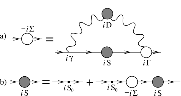
Fig. 2.2: The Dyson-Schwinger equation for the electron propagator.

The structure of Eq. (2.25) allows one to rewrite it in terms of the fermion self energy, $-i\Sigma^{f}(x,y)$, defined such that

$$(i\not\!\partial-m_{0}^{f})\,S^{f}(x,y)-\int d^{\rm d}z_{1}\,\Sigma^{f}(x,z_{1})\,S^{f}(z_{1},y)=\delta^{\rm d}(x-y)~{}$$ (2.26)

and hence satisfying

$$-i\Sigma^{f}(x,y)=(e_{0}^{f})^{2}\int\,d^{\rm d}z_{1}\,d^{\rm d}z_{2}\,\gamma_{\mu}D^{\mu\nu}(x,z_{1})S^{f}(x,z_{2})\Gamma^{f}_{\nu}(z_{1};z_{2},y)~{}.$$ (2.27)

The equation for the fermion self-energy is represented diagrammatically in Fig. 2.2a) while part b) of this figure shows the definition of the fermion self-energy ($-i\Sigma^{f}(p)$) in terms of the fermion propagator $S^{f}(p)$ with $S^{f}_{0}(p)=1/(\mbox{$\not\!p$}-m^{f}_{0})$ the bare fermion propagator. Again, the momentum-space form for the proper fermion self-energy ($-i\Sigma^{f}$) is easily obtained from Fig. 2.2a) using the usual Feynman rules [or equivalently from Fourier transforming Eq. (2.27)] and can be written as

$$-i\Sigma^{f}(p)=(e_{0}^{f})^{2}\int\frac{d^{\rm d}\ell}{(2\pi)^{\rm d}}(i\gamma_{\mu})(iS^{f}(\ell))(iD^{\mu\nu}(p-\ell))(i\Gamma^{f}_{\nu}(\ell,p))\;.$$ (2.28)

From Fig. 2.2b) or, equivalently, from Eq. (2.26), we can solve for $S^{f}(p)$ to give $S^{f}(p)=1/[(S^{f}_{0})^{-1}-\Sigma^{f}(p)]=1/[\mbox{$\not\!p$}-m^{f}_{0}-\Sigma^{f}(p)]$.

Unrenormalised Dyson-Schwinger equation for the Fermion-Photon Vertex.       This equation can be derived in a similar way. For completeness, we present it here in momentum space where it is most concisely written (Bjorken and Drell, 1965, pp. 291-293):

$$i\Gamma^{f}_{\mu}(p^{\prime},p)=i\gamma_{\mu}+\sum_{g}\int\frac{d^{\rm d}\ell}{(2\pi)^{\rm d}}(iS^{g}(p^{\prime}+\ell))(i\Gamma^{g}_{\mu}(p^{\prime}+\ell,p+\ell))(iS^{g}(p+\ell))K^{gf}(p+\ell,p^{\prime}+\ell,\ell)~{},$$ (2.29)

where $K$ is referred to as the fermion-antifermion scattering kernel. The diagrammatic representation of this is given in Fig. 2.3.

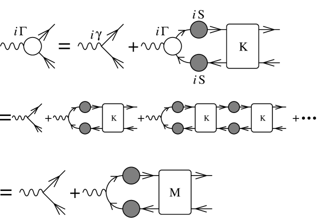
Fig. 2.3: The Dyson-Schwinger equation for the electron-photon proper vertex.

Clearly, $\Gamma^{\mu}$ is coupled to the fermion 2-point function [the fermion propagator $S$] and also to a fermion-antifermion scattering amplitude denoted by $M$, a 4-point function, which itself satisfies an integral equation (Bjorken and Drell, 1965, pp. 293-298) and this illustrates the general rule again. The amplitude $M$ is 1-PI with respect to the fermion lines and does not contain any fermion-antifermion annihilation contributions [i.e., no intermediate single photon state] since these would not be 1-PI contributions to $\Gamma^{f\mu}$ with respect to the photon line. In an obvious shorthand notation we see from Fig. 2.3 that $M=K+K(iS)^{2}K+K(iS)^{2}K(iS)^{2}K+\cdots=K+K(iS)^{2}M$. Hence it follows that the fermion-antifermion scattering kernel $K$ has no annihilation contributions and is 2-PI with respect to the fermion-antifermion pair of lines. The latter requirement ensures that there is no double counting when $(iS)^{2}K$ is iterated to form $M$. It then follows that to lowest order in perturbation theory $M^{fg}=K^{fg}=\delta^{fg}(e_{0}^{f})^{2}(i\gamma_{\mu})(iD^{\mu\nu}_{0})(i\gamma_{\nu})$, where $D_{0}$ is the bare photon propagator. The simplest so-called ladder approximation consists of approximating $M$ by iterating the lowest order perturbative contribution for the kernel $K$ together with the replacement of the fermion propagators by their perturbative form; i.e., $S^{f}_{0}(p)=1/[\mbox{$\not\!p$}-m^{f}_{0}]$.

Just as there was a WTI for photon vacuum polarisation [i.e., $q_{\mu}\Pi^{\mu\nu}(q)=0$] there is a WTI which relates the fermion propagator to the proper fermion-photon vertex [see, for example, Itzykson and Zuber (1980, pp. 407-411)]

$$k_{\mu}\Gamma^{f\mu}(p+k,p)=(S^{f})^{-1}(p+k)-(S^{f})^{-1}(p)\;.$$ (2.30)

Renormalisation of the Equations.       Once the technique for deriving the unrenormalised equations is known then the renormalised equations follow. Essentially, one need only modify the action of the theory to include the necessary counterterms and repeat the above procedure. For the purposes of this discussion we will temporarily adopt a notation similar to that used in Bjorken and Drell (1965, pp. 283-376), where the renormalised action and the quantities derived from it are denoted by a tilde to distinguish these from the unrenormalised quantities.

In $N_{f}$ flavour QED_d one has the following [infinite] renormalisation constants (Dyson, 1949): the fermion wave function renormalisation, $Z_{2}$, which relates the bare fermion field to the renormalised one; the photon wave function renormalisation, $Z_{3}$; and the vertex renormalisation, $Z_{1}$, which relates the bare and renormalised charge:

$$\begin{array}[]{ccc}\psi^{f}_{0}=\sqrt{Z^{f}_{2}}\psi^{f}~{};&A^{\mu}_{0}=\sqrt{Z_{3}}A^{\mu}~{};&e_{0}^{f}=\displaystyle\frac{Z^{f}_{1}}{Z^{f}_{2}\sqrt{Z_{3}}}e^{f}~{}.\end{array}$$ (2.31)

A fundamental requirement and consequence of gauge invariant regularisation and renormalisation of the theory is the Ward Identity (Ward, 1950; Takahashi, 1957), which leads to

$$Z^{f}_{1}=Z^{f}_{2}~{}.$$ (2.32)

This identity together with the multiplicative nature of renormalisation ensures that the WTIs are preserved in the renormalised theory. In addition it ensures charge universality; i.e., that different species of fermion have their charge renormalised by the same multiplicative factor. The QED_d renormalised action [i.e., including the counterterms] is obtained from Eq. (2.1) by identifying $\tilde{S}_{\xi}[\mbox{$\overline{\psi}$},\psi,A^{\mu}]\equiv S_{\xi}[\mbox{$\overline{\psi}$}_{0},\psi_{0},A^{\mu}_{0}]$ and making use of Eq. (2.31). Hence the renormalised action is given by

$$\tilde{S}_{\xi}[\mbox{$\overline{\psi}$},\psi,A_{\mu}]=\int\,d^{\rm d}x\;\left[\,\sum_{f=1}^{N_{f}}\,\left[Z^{f}_{2}\mbox{$\overline{\psi}$}^{f}\left(i\mbox{$\not\!\partial$}-m_{0}^{f}\right)\psi^{f}+Z^{f}_{1}e^{f}\mbox{$\overline{\psi}$}^{f}\mbox{$\not\!\!A$}\psi^{f}\right]-\frac{Z_{3}}{4}F_{\mu\nu}F^{\mu\nu}-\frac{Z_{3}}{2\xi_{0}}(\partial_{\mu}A^{\mu})^{2}\right]$$

$$=\int\,d^{\rm d}x\;\left[\,\sum_{f=1}^{N_{f}}\,\mbox{$\overline{\psi}$}^{f}\left(i\mbox{$\not\!\partial$}-m^{f}+e^{f}\mbox{$\not\!\!A$}\right)\psi^{f}-\frac{1}{4}F_{\mu\nu}F^{\mu\nu}-\frac{1}{2\xi}(\partial_{\mu}A^{\mu})^{2}\right.$$

$$\left.+\sum_{f}\left[(Z^{f}_{2}-1)\mbox{$\overline{\psi}$}^{f}i\mbox{$\not\!\partial$}\psi^{f}-\delta m^{f}~{}\mbox{$\overline{\psi}$}^{f}\psi^{f}+\delta e^{f}~{}\mbox{$\overline{\psi}$}^{f}\mbox{$\not\!\!A$}\psi^{f}\right]-\frac{(Z_{3}-1)}{4}F_{\mu\nu}F^{\mu\nu}\right]~{},$$ (2.33)

where the four terms in the last line of this equation are called counterterms and depend on both the regularisation parameter and the renormalisation point. We see that $\delta m^{f}\equiv m^{f}_{B}-m^{f}\equiv Z^{f}_{2}m^{f}_{0}-m^{f}$ and $\delta e^{f}\equiv e^{f}_{B}-e^{f}\equiv(Z^{f}_{1}-1)e^{f}$. There is no gauge-parameter counterterm since $\xi_{0}=Z_{3}\xi$, which follows from Eq. (2.31) and from the WTI, $q_{\mu}\Pi^{\mu\nu}=0$, which ensures that vacuum polarisation only affects the transverse part of the photon propagator. We will refer to $\mbox{$\overline{\psi}$}^{f}_{0},\psi^{f}_{0},A^{\mu}_{0},m^{f}_{0},e^{f}_{0},$ and $\xi_{0}$ as the bare quantities, although occasionally in the literature this term is also used to describe $m^{f}_{B}$ and $e^{f}_{B}$. This is discussed for example in Collins (1984, pp. 10-11). The renormalised [i.e., physical ] fermion masses and charges are $m^{f}$ and $e^{f}$, respectively, and $\xi$ is the renormalised gauge parameter.

The renormalised action, $\tilde{S}_{\xi}$, will lead immediately to the corresponding renormalised generating functionals $\tilde{\cal Z}$, $\tilde{\cal G}$, and $\tilde{\Gamma}$, from Eqs. (2.3), (2.8), and (2.12) respectively. Using the same steps as before these in turn lead to the renormalised Green’s functions $\tilde{D}^{\mu\nu}$, $\tilde{S}^{f}$, $\tilde{\Gamma}_{\mu}^{f}$, $\tilde{K}^{fg}$, etc. The renormalisation is carried out subject to the following boundary conditions on renormalised quantities:

$$\left.(\tilde{S}^{f})^{-1}(p)\right|_{p^{2}=(m^{f})^{2}}=\mbox{$\not\!p$}-m^{f}\;,\;\;\left.\tilde{\Gamma}^{f\mu}(p,p)\right|_{\mbox{\footnotesize$\not\!p$}=m^{f}}=\gamma^{\mu}\;,\;\;\tilde{\Pi}(0)=0\;,$$ (2.34)

together with the definition of the renormalised fermion and photon propagators:

$$(\tilde{S}^{f})^{-1}(p) = \mbox{$\not\!p$}-m^{f}-\tilde{\Sigma}^{f}(p)~{},$$

$$\tilde{D}^{\mu\nu}(q) = \frac{-g^{\mu\nu}+(q^{\mu}q^{\nu}/(q^{2}+i\epsilon))}{q^{2}+i\epsilon}\frac{1}{1+\tilde{\Pi}(q^{2})}-\xi\frac{q^{\mu}q^{\nu}}{(q^{2}+i\epsilon)^{2}}~{}.$$ (2.35)

The first condition in Eq. (2.34) specifies that the renormalised fermion propagator, $\tilde{S}^{f}(p)$, has a pole of residue one at the physical fermion mass $m^{f}$; i.e., that $\tilde{\Sigma}^{f}(p)=0$ at $p^{2}=(m^{f})^{2}$. The second condition ensures that when an on-shell fermion of flavour $f$ is probed with a zero-momentum photon we measure the physical charge, $e^{f}$. The notation $\mbox{$\not\!p$}=m^{f}$ means that all factors of $\not\!p$ are replaced by $m^{f}$, which is equivalent to having $\tilde{\Gamma}^{f\mu}$ act on a free spinor at the fermion mass pole, $p^{2}=(m^{f})^{2}$. Note that for nondegenerate fermion masses [i.e., $m^{f^{\prime}}\neq m^{f}$] this boundary condition introduces a subtle distinction between $\tilde{\Gamma}^{f}_{\mu}$ and $\tilde{\Gamma}^{f^{\prime}}_{\mu}$, since otherwise these vertices would be identical. The last boundary condition ensures that an on-shell photon has a pole at $p^{2}=0$ with unit residue after vacuum polarisation corrections.

There are some subtle difficulties with these boundary conditions due to infrared divergences but these are readily taken care of by introducing a small photon mass as discussed, e.g., in Itzykson and Zuber (1980, pp. 413-414). It should be noted that this choice of boundary conditions corresponds to the particular choice of the on-shell renormalisation point, which is the usual choice for QED. We know, however, from renormalisation group arguments, that this choice is in fact arbitrary. Since QCD is believed to be confining, it has no corresponding natural choice of renormalisation point.

Following these arguments gives, in place of Eq. (2.17),

$$\left.e^{f}\,\tilde{\Gamma}^{f}_{\mu}(x;y,z)=\frac{\delta}{\delta A^{\mu}(x)}\frac{\delta^{2}\tilde{\Gamma}}{\delta\mbox{$\overline{\psi}$}^{f}(y)\delta\psi^{f}(z)}\right|_{0=A_{\mu}=\psi=\overline{\psi}}~{}.$$ (2.36)

Similarly, in place of Eqs. (2.18) and (2.19), we find

$$(\tilde{D}^{-1})^{\mu\nu}(x,y) = \left.\frac{\delta^{2}\tilde{\Gamma}}{\delta A^{\mu}(x)\delta A^{\nu}(y)}\right|_{A_{\mu}=\psi=\overline{\psi}=0}=Z_{3}\left[\partial_{\rho}\partial^{\rho}g_{\mu\nu}-\left(1-\frac{1}{\xi_{0}}\right)\partial_{\mu}\partial_{\nu}\right]\delta^{\rm d}(x-y)+\Pi^{\prime}_{\mu\nu}(x,y)$$ (2.37)

$$= Z_{3}\left[\partial_{\rho}\partial^{\rho}g_{\mu\nu}-\partial_{\mu}\partial_{\nu}\right]\delta^{\rm d}(x-y)+\frac{1}{\xi}\partial_{\mu}\partial_{\nu}\delta^{\rm d}(x-y)+\Pi^{\prime}_{\mu\nu}(x,y)$$

where we have [c.f., Eq. (2.19)]

$$\Pi^{\prime}_{\mu\nu}(x,y)=i\sum_{f}Z_{1}^{f}(e^{f})^{2}\int\,d^{\rm d}z_{1}\,d^{\rm d}z_{2}\,{\rm tr}\left[\gamma_{\mu}\tilde{S}^{f}(x,z_{1})\tilde{\Gamma}_{\nu}(y;z_{1},z_{2})\tilde{S}^{f}(z_{2},x)\right]~{}.$$ (2.38)

In momentum space we then define $\Pi^{\prime}_{\mu\nu}(q)\equiv(-g_{\mu\nu}q^{2}+q_{\mu}q_{\nu})\Pi^{\prime}(q^{2})$ and hence it follows from the momentum space form of Eq. (2.37) and from Eq. (2.35) that $\tilde{\Pi}(q^{2})=(Z_{3}-1)+\Pi^{\prime}(q^{2})$. From the boundary condition $\tilde{\Pi}(0)=0$ we find that

$$Z_{3}=1-\Pi^{\prime}(0)$$ (2.39)

and so finally that

$$i\tilde{\Pi}_{\mu\nu}(q)=i(-g_{\mu\nu}q^{2}+q_{\mu}q_{\nu})\tilde{\Pi}(q^{2})=i(-g_{\mu\nu}q^{2}+q_{\mu}q_{\nu})[\Pi^{\prime}(q^{2})-\Pi^{\prime}(0)]~{}.$$ (2.40)

Note that $q_{\mu}\Pi^{\prime\mu\nu}=0$ [assuming a covariant, gauge-invariant regularisation scheme] just as before, and hence we have seen that the WTI for the vacuum polarisation has survived renormalisation; i.e., $q_{\mu}\tilde{\Pi}^{\mu\nu}=0$, as expected.

Repeating the same arguments for the fermion self-energy we find Eq. (2.25) becomes

$$Z_{2}^{f}(i\not\!\partial-m_{0}^{f})\,\tilde{S}^{f}(x,y)-\int\,d^{\rm d}z_{1}\Sigma^{f\prime}(x,z_{1})\tilde{S}^{f}(z_{1},y)=\delta^{\rm d}(x-y)~{},$$ (2.41)

where

$$-i\Sigma^{f\prime}(x,y)=Z_{1}^{f}(e^{f})^{2}\int\,d^{\rm d}z_{1}\,d^{\rm d}z_{2}\,\gamma_{\mu}\tilde{D}^{\mu\nu}(x,z_{1})\tilde{S}^{f}(x,z_{2})\tilde{\Gamma}_{\nu}^{f}(z_{1};z_{2},y)~{}.$$ (2.42)

In momentum space we have $(\tilde{S}^{f})^{-1}(p)=Z_{2}^{f}(\mbox{$\not\!p$}-m^{f}_{0})-\Sigma^{f\prime}(p)=\mbox{$\not\!p$}-m^{f}-\tilde{\Sigma}^{f}(p)$. Using Lorentz invariance allows us to decompose $\Sigma^{f\prime}$ into Dirac-vector and -scalar pieces: $\Sigma^{f\prime}(p)=\Sigma_{d}^{f\prime}(p^{2})\mbox{$\not\!p$}+\Sigma_{s}^{f\prime}(p^{2})$; and similarly for $\tilde{\Sigma}^{f}$. Hence we find $\tilde{\Sigma}_{d}^{f}(p^{2})=\Sigma_{d}^{f\prime}(p^{2})-(Z_{2}^{f}-1)$ and $\tilde{\Sigma}_{s}^{f}(p^{2})=\Sigma_{s}^{f\prime}(p^{2})+(Z_{2}^{f}m_{0}^{f}-m^{f})$. Hence the boundary condition $\tilde{\Sigma}^{f}(p)=0$ at $p^{2}=(m^{f})^{2}$ gives

$$Z_{2}^{f}=1+\Sigma_{d}^{f\prime}((m^{f})^{2})\;\;,\;\;\;\;m_{0}^{f}=\left[m^{f}-\Sigma_{s}^{f\prime}((m^{f})^{2})\right]/Z_{2}^{f}~{}.$$ (2.43)

Then we have $\tilde{\Sigma}^{f}(p)=\tilde{\Sigma}_{d}^{f}(p^{2})\mbox{$\not\!p$}+\tilde{\Sigma}_{s}^{f}(p^{2})$, where

$$\tilde{\Sigma}_{d}^{f}(p^{2})=\Sigma_{d}^{f\prime}(p^{2})-\Sigma_{d}^{f\prime}((m^{f})^{2})\;\;,\;\;\;\;\tilde{\Sigma}_{s}^{f}(p^{2})=\Sigma_{s}^{f\prime}(p^{2})-\Sigma_{s}^{f\prime}((m^{f})^{2})~{}.$$ (2.44)

If we introduce the notation $(\tilde{S}^{f})^{-1}(p)=A^{f}(p^{2})\mbox{$\not\!p$}-B^{f}(p^{2})=(Z^{f})^{-1}(p^{2})[\mbox{$\not\!p$}-M^{f}(p^{2})]$, then this leads to the renormalised DSE for the fermion propagator in the form that we use in later sections:

$$A^{f}(p^{2})=(Z^{f})^{-1}(p^{2})=1-\tilde{\Sigma}_{d}^{f}(p^{2})\;\;,\;\;\;\;B^{f}(p^{2})=(Z^{f})^{-1}(p^{2})M^{f}(p^{2})=m^{f}+\tilde{\Sigma}_{s}^{f}(p^{2})~{}.$$ (2.45)

For the fermion-photon proper vertex we have, in place of Eq. (2.29),

$$\tilde{\Gamma}^{f}_{\mu}(p^{\prime},p) = Z_{1}^{f}\gamma_{\mu}-\int\frac{d^{\rm d}q}{(2\pi)^{\rm d}}\tilde{S}^{f}(p^{\prime}+q)\tilde{\Gamma}^{f}_{\mu}(p^{\prime}+q,p+q)\tilde{S}^{g}(p+q)\tilde{K}^{fg}(p+q,p^{\prime}+q,q)~{}$$ (2.46)

$$\equiv Z_{1}^{f}\gamma_{\mu}+\Lambda^{f\prime}_{\mu}(p^{\prime},p)\equiv\gamma_{\mu}+\tilde{\Lambda}^{f}_{\mu}(p^{\prime},p)~{},$$

which also defines both $\Lambda^{f\prime}_{\mu}$ and $\tilde{\Lambda}^{f}_{\mu}$. Hence, we have $\tilde{\Lambda}^{f}_{\mu}(p^{\prime},p)=\Lambda^{f\prime}_{\mu}(p^{\prime},p)+(Z_{1}^{f}-1)\gamma_{\mu}$ and from the boundary condition for the vertex in Eq. (2.34) we find

$$\left.(Z_{1}^{f}-1)\gamma_{\mu}=-\Lambda^{f\prime}_{\mu}(p,p)\right|_{\mbox{\footnotesize$\not\!p$}=m^{f}}~{},$$ (2.47)

which gives finally that

$$\tilde{\Lambda}^{f}_{\mu}(p^{\prime},p)=\Lambda^{f\prime}_{\mu}(p^{\prime},p)-\Lambda^{f\prime}_{\mu}(p,p)\left|{}_{\mbox{\footnotesize$\not\!p$}=m^{f}}\right.\;.$$ (2.48)

Since $(e^{f}\tilde{\Gamma}_{\mu}^{f})$, $(\tilde{D}^{-1})_{\mu\nu}$, and $(\tilde{S}^{f})^{-1}$ are all obtained by differentiating $\tilde{\Gamma}[\mbox{$\overline{\psi}$},\psi,A_{\mu}]$, then it follows, for example, from Eqs. (2.17,2.31,2.33,2.36) that $(e^{f}_{0}\Gamma^{f}_{\mu})=(Z^{f}_{2}\sqrt{Z_{3}})^{-1}(e^{f}\tilde{\Gamma}_{\mu}^{f})$. Similarly, $S^{f}=Z^{f}_{2}\tilde{S}^{f}$ and $D_{\mu\nu}=Z_{3}\tilde{D}_{\mu\nu}$. Thus from the unrenormalised WTI of Eq. (2.30) we find for the renormalised quantities $(Z_{2}^{f}/Z_{1}^{f})k_{\mu}\tilde{\Gamma}^{f\mu}(p+k,p)=(\tilde{S}^{f})^{-1}(p+k)-(\tilde{S}^{f})^{-1}(p)$, which implies that since the theory is renormalisable then $Z_{1}^{f}$ and $Z_{2}^{f}$ can only differ by a finite amount. In fact from the boundary conditions in Eq. (2.34) we see immediately that we must have $Z_{1}^{f}=Z_{2}^{f}$, as was stated earlier. The WTI implies the Ward identity, which can be written as $\tilde{\Gamma}_{\mu}^{f}(p,p)=\partial(\tilde{S}^{f})^{-1}(p)/\partial p^{\mu}$. [For ease of comparison with Bjorken and Drell (1965), pp. 311-312, note that, e.g., $\tilde{\Lambda}$ and $\tilde{\Pi}$ used here correspond to $\Lambda_{c}$ and $e^{2}\Pi_{c}$, respectively, in that work.]

In repeating the previous arguments and deriving the above renormalised equations it soon becomes apparent that $Z$-factors are only introduced when bare propagators or vertices appear in the DSE. We have not discussed details of the various regularisation schemes but it should be clear that all of the regularisation-parameter dependence has been absorbed into these factors. Let $\Lambda$ denote a generic regularisation parameter such that $\Lambda\to\infty$ as the regularisation is removed, e.g., $\Lambda$ might denote a simple momentum cut-off or using dimensional regularisation, where ${\rm d}=4-\epsilon$, we would identify $\Lambda=1/\epsilon$, etc. Then the $Z$-factors are functions of the regularisation parameter and the renormalisation point; i.e., $Z_{2}\equiv Z_{2}(\Lambda,\mu)$, etc. For $m+n>3$, where $m$ is the [even] number of external fermion legs and $n$ the number of external photon legs, it can be shown that the unrenormalised Greens functions can be decomposed into an infinite sum of skeleton diagrams each of which is made up only of combinations of $S^{f}$, $D^{\mu\nu}$, and $e_{0}\Gamma^{f}_{\mu}$. However, we have seen that in the renormalised theory the quantities $e^{f}_{0}\Gamma^{f}_{\mu}$, $D^{\mu\nu}$, and $S^{f}$ are simply replaced by the renormalised quantities $e^{f}\tilde{\Gamma}^{f}_{\mu}$, $\tilde{D}^{\mu\nu}$, and $\tilde{S}^{f}$. Hence, for Green’s functions with $m+n>3$ we simply replace the skeleton expansion for the unrenormalised Greens function by the same skeleton expansion with the renormalised quantities. This is the meaning of $\tilde{K}$ in Eq. (2.46), for example. This completes the renormalisation program for QED. A more detailed discussion of the skeleton expansion and associated proof of renormalisability can be found in Bjorken and Drell (1965).

Review.       We have illustrated the general technique for obtaining the DSEs for a field theory and have demonstrated by example the nature of the hierarchy of equations; i.e, that the equations couple a given $n$-point function to adjacent $n$-point functions in an infinite tower of coupled equations. We have also discussed in some detail the renormalisation of these equations. As was already noted, choices of subtraction point [i.e., renormalisation point] other than the on-shell subtraction point of Eq. (2.34) are possible. From the previous discussion it is clear that such a change can simply be absorbed as a finite rescaling of the renormalised charges and masses whilst leaving the physical content of the theory unchanged. This observation is the basis of renormalisation group studies of field theories. We note in passing that with a suitably unconventional choice of subtraction scheme one can find $Z_{1}^{f}\neq Z_{2}^{f}$, although this is not the case in standard approaches [of course, this has no physical significance]. The renormalised masses and charges in QED₄ only correspond to the physical ones when the on-shell renormalisation point is used. There is no corresponding on-shell renormalisation in QCD, since QCD is believed to be a confining theory. We have now introduced all of the concepts that are necessary for the discussion of DSE studies of QED_d in Secs. 3 and 4. For our discussion of QCD in Sec. 2.2 we simply point out the added complications due to the non-Abelian nature of the theory.

2.2 Quantum Chromodynamics [QCD]

QCD is a non-Abelian gauge theory [based on the fundamental representation of the group $SU(3)$], which leads to significantly different behaviour than that shown by the Abelian theory of QED [based on the group $U(1)$]. In simple terms this arises because the non-Abelian gauge fields are self-interacting. The basic Lagrangian of QCD is given by

$$S[\mbox{$\overline{\psi}$},\psi,A_{\mu}]=\int\,d^{\rm d}x\;\left[\,\sum_{f=1}^{N_{f}}\,\mbox{$\overline{\psi}$}^{f}\left(i\mbox{$\not\!\!D$}-m_{0}^{f}\right)\psi^{f}-\frac{1}{4}F_{\mu\nu a}F^{\mu\nu}_{a}\right]~{},$$ (2.49)

where

$$F^{\mu\nu}_{a} = \partial^{\mu}A^{\nu}_{a}-\partial^{\nu}A^{\mu}_{a}+g_{0}f_{abc}A^{\mu}_{b}A^{\nu}_{c}~{},$$ (2.50)

$$D^{\mu} = \partial^{\mu}-ig_{0}A^{\mu}_{a}t_{a}=\partial^{\mu}-ig_{0}A^{\mu}~{}.$$ (2.51)

and where $A^{\mu}\equiv A^{\mu}_{a}t_{a}$. The fields $A^{\mu}_{a}$ are the gluon fields and $\psi^{f}$ are the quark fields, where $f=1,\cdots,N_{f}$ is the quark flavour index. The indices $a=1,\cdots,8$ are colour indices and summation over repeated indices is to be understood. We use standard conventions [e.g., Ynduráin (1993), Muta (1987)] where $t_{a}\equiv\lambda_{a}/2$ and the hermitian [Gell-Mann] matrices $\lambda_{a}$ are the generators of $SU(3)$. The $\lambda_{a}$ matrices satisfy ${\rm tr}(\lambda_{a}\lambda_{b})=2\delta_{ab}$ and $[\lambda_{a},\lambda_{b}]=2if_{abc}\lambda_{c}$, which leads to ${\rm tr}(t_{a}t_{b})=T_{F}\delta_{ab}=\delta_{ab}/2$ and $[t_{a},t_{b}]=f_{abc}t_{c}\equiv-C_{abc}t_{c}$. [Note that Itzykson and Zuber (1980, pp. 563-567) define instead antihermitian matrices $t_{a}\equiv i\lambda_{a}/2$]. We can write, e.g., $(1/4)F^{\mu\nu}_{a}F_{\mu\nu a}=(1/2){\rm tr}(F^{\mu\nu}F_{\mu\nu})$, where $F^{\mu\nu}\equiv t_{a}F^{\mu\nu}_{a}=\partial^{\mu}A^{\nu}-\partial^{\nu}A^{\mu}-ig_{0}[A^{\mu},A^{\nu}]=(i/g_{0})[D^{\mu},D^{\nu}]$. For $SU(N)$, the Casimir invariants $C_{A},C_{F}$, and $T_{F}$ take on the values $C_{A}=N$, $C_{F}=(N^{2}-1)/2N$, and $T_{F}=1/2$.

As for QED, it is necessary to remove the infinite gauge-volume problem due to integrations over gauge-equivalent field configurations. This is remedied by the prescription of Faddeev and Popov (1967) and has the added complication that in order to maintain gauge invariance and unitarity in covariant gauges it is necessary to introduce unphysical auxiliary fields ($\mbox{$\overline{\omega}$}_{a},\omega_{a}$). These are anticommuting spin-zero fields called ghost fields and it is also necessary to integrate over these fields in order to define the generation functional ${\cal Z}$ for QCD. A technical point, which we shall neglect henceforth, is the fact that the Faddeev-Popov gauge-fixing procedure only uniquely specifies the gauge field configuration with respect to infinitesimal local gauge transformations. Under finite transformations gauge-equivalent field configurations remain and are referred to as Gribov copies [see, e.g., Itzykson and Zuber (1980, pp. 574-582) and Gribov (1979)]. It is possible to choose ghost-free gauge-fixing prescriptions such as the axial gauge, where $n\cdot A=0$ for some spacelike four-vector $n^{\mu}$, ($n^{2}<0$). The cases $n^{2}>0$ and $n^{2}=0$ are referred to as the temporal and light-cone gauges, respectively. The disadvantages of such a choice are that Lorentz invariance is now broken explicitly and unphysical singularities are present in the denominators of momentum-space propagators; i.e., when $p\cdot n=0$.

The quantum field theory associated with Eq. (2.49) is defined for covariant gauges by the generating functional

$${\cal Z}[\mbox{$\overline{\eta}$},\eta,J_{\mu},\mbox{$\overline{\xi}$},\xi]=$$

$$\int\,d\mu(\mbox{$\overline{\psi}$},\psi,A,\mbox{$\overline{\omega}$},\omega)\,\exp\Big{(}iS_{\xi}[\mbox{$\overline{\psi}$},\psi,A_{\mu},\mbox{$\overline{\omega}$},\omega]+i\int\,d^{\rm d}x\;\left[\mbox{$\overline{\psi}$}^{f}\eta^{f}+\mbox{$\overline{\eta}$}^{f}\psi^{f}+A_{\mu a}J^{\mu}_{a}+\mbox{$\overline{\omega}$}_{a}\xi_{a}+\mbox{$\overline{\xi}$}_{a}\omega_{a}\right]\Big{)}$$

where

$$S_{\xi}[\mbox{$\overline{\psi}$},\psi,A_{\mu},\mbox{$\overline{\omega}$},\omega]=S[\mbox{$\overline{\psi}$},\psi,A_{\mu}]+\int\,d^{\rm d}x\,\left[(\partial_{\mu}\mbox{$\overline{\omega}$}_{a})(\delta_{ab}\partial^{\mu}-g_{0}f_{abc}A^{\mu}_{c})\omega_{b}-\frac{1}{2\xi_{0}}\left(\partial_{\mu}A^{\mu}\right)^{2}\right]~{},$$ (2.53)

where $\xi_{0}$ is the bare gauge fixing parameter. The Faddeev-Popov technique for non-Abelian gauge fields [as well as the gauge fixing procedure for QED] can be understood in terms of the more general class of Becchi-Rouet-Stora [BRS] transformations. These are a generalisation of the local gauge transformations to include the ghost and gauge-fixing terms. The Slavnov-Taylor identities [STIs] can be derived from the BRS invariance of QCD and correspond to the WTIs of QED. It can be shown that requiring BRS invariance of a gauge theory automatically generates both the ghosts [where appropriate] and the gauge fixing as well as ensuring the gauge-invariance of physical observables, [see e.g., Pokorski (1987) pp. 64-85 and Pascual and Tarrach (1984) and references therein].

Just as for QED we introduce appropriate counterterms into the QCD action in Eq. (2.53) in order to define the QFT and then apply appropriate boundary conditions at the chosen renormalisation point [a momentum scale that we refer to as $\mu$]. Since the renormalisation point, $\mu$, is arbitrary, physical observables must be independent of its choice. In other words, hadronic masses and cross-sections must be renormalisation-point independent even though individual Green’s functions [e.g., the quark and gluon propagators] may not be. In analogy with QED we identify the renormalised action using $\tilde{S}_{\xi}[\mbox{$\overline{\psi}$},\psi,A^{\mu},\mbox{$\overline{\omega}$},\omega]\equiv S_{\xi}[\mbox{$\overline{\psi}$}_{0},\psi_{0},A^{\mu}_{0},\mbox{$\overline{\omega}$}_{0},\omega_{0}]$ together with the relations [see, e.g., Ynduráin (1993) pp. 45-83]

$$\begin{array}[]{cccc}\psi^{f}_{0}=\sqrt{Z_{F}}\psi^{f}~{};&A^{\mu}_{a0}=\sqrt{Z_{B}}A^{\mu}_{a}~{};&\omega_{a0}=\sqrt{Z_{\omega}}\omega_{a}~{};&g_{0}=\displaystyle Z_{g}g~{}.\end{array}$$ (2.54)

As a consequence of gauge invariant regularisation and renormalisation of the theory the STIs are maintained, which leads to the fact that all quark colours have the same $Z^{f}_{F}$ and that all gluons and ghosts have the same $Z_{B}$ and $Z_{\omega}$ respectively. In analogy with QED we see that $\xi_{0}=Z_{B}\xi$, since only the transverse part of the gluon propagator is modified by vacuum polarisation [i.e., $q_{\mu}\tilde{\Pi}^{\mu\nu}=0$]. Here, $Z_{g}$ plays the role of the QED combination $Z_{1}^{f}/Z_{2}^{f}\sqrt{Z_{3}}$, so that in place of $Z_{1}^{f}$ in QED we have $Z^{f}_{\Gamma}\equiv Z_{g}Z^{f}_{F}\sqrt{Z_{B}}$ in QCD. The STIs also imply that the same renormalisation constant $Z_{g}$ applies to the quark-gluon, ghost-gluon, three-gluon, and four-gluon vertices. The STIs are the reason that we do not need other independent renormalisation constants for these couplings, [see, e.g., Itzykson and Zuber (1980, pp. 593-594) and Muta (1987, pp. 158-179)]. We can define $\delta m^{f}\equiv m^{f}_{B}-m^{f}\equiv Z^{f}_{F}m^{f}_{0}-m^{f}\equiv(Z^{f}_{F}Z^{f}_{m}-1)m^{f}$ as for QED, where the last result follows from the definition of $Z^{f}_{m}$ by $m^{f}_{0}\equiv Z^{f}_{m}m^{f}$.

The derivation of the unrenormalised and renormalised DSEs proceeds in an analogous way to that for QED and, as already stated, these are a direct result of the BRS invariance of the theory. In Fig. 2.4 we show the DSE for the quark self-energy. The graphical representation of the quark propagator DSE is the same as that for the electron given in Fig. 2.2b). Figure 2.5 specifies the Dyson-Schwinger equation for the gluon propagator and can be compared with the photon DSE in Fig. 2.1. The symmetrisation factors of 1/2 and 1/6 arise from the usual Feynman rules, which also require a negative sign [unshown] to be included for every fermion and ghost loop. In Fig. 2.6 we show the quark-gluon proper vertex DSE. The notation is analogous to that used for the QED fermion-photon vertex in Fig. 2.3; i.e., the amplitudes $M,M^{\prime},M^{\prime\prime}$, and $M^{\prime\prime\prime}$ are 1-PI with respect to all external legs and do not contain any single-gluon intermediate states.

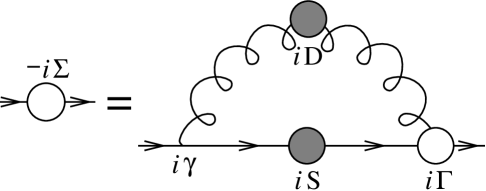
Fig. 2.4: The Dyson-Schwinger equation for the quark self-energy.

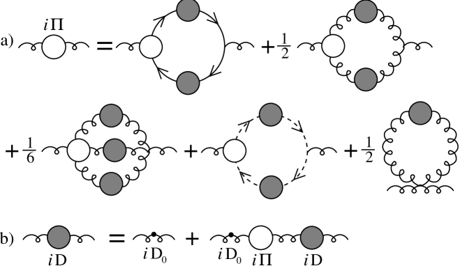
Fig. 2.5: The Dyson-Schwinger equation for the gluon propagator. [Here and below the broken line represents the propagator for the ghost field.]

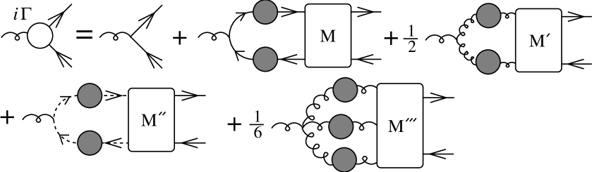
Fig. 2.6: The quark-gluon vertex Dyson-Schwinger equation.

The difficult challenge is to find an Ansatz for the unknown renormalised propagators, vertices, etc., of QCD which satisfy the DSEs and respect the STIs of the theory. Progress can be made by satisfying a subset of the DSEs and STIs and then supplementing these with information gleaned from lattice gauge theory, phenomenology, etc. The test of such a scheme is to enlarge the set of DSEs considered and look for a decreased dependence on the phenomenological input. Since the most significant difficulties in QCD arise in the gluon sector this is the natural place to appeal to phenomenology while attempting to construct explicit solutions and maintain important symmetries in the quark sector. Two symmetries of particular importance are gauge invariance and chiral symmetry.

Note: Having completed the discussion of renormalisation, we now dispense with the tilde notation for renormalised Green’s functions, self-energies, vacuum polarisations, etc. In analogy with the QED case we then denote the renormalised quark and gluon propagators [in momentum space] by $S^{f}(p)$ and $D^{\mu\nu}_{ab}(p)\equiv\delta_{ab}D^{\mu\nu}(p)$ respectively, ($a,b=1,...,8$ are $SU(3)$ colour indices. For a covariant gauge the renormalised gluon propagator and quark propagators have forms identical to those in Eq. (2.35). We can write for the proper quark-gluon vertex $\Gamma^{\mu}_{a}(p^{\prime},p)\equiv t_{a}\Gamma^{\mu}(p^{\prime},p)$.

The renormalised quantities $S^{f}$, $\Sigma^{f}$, $D$, $\Pi$, $\Gamma^{f}$, $\xi$, $g$, $m^{f}$, etc. have a dependence on the both the renormalisation point $\mu$ and the gauge parameter $\xi$ in general, but we do not explicitly indicate these for notational brevity. The renormalised coupling $g$ is related to the running coupling constant $\alpha_{s}(Q^{2})=g^{2}(Q^{2})/4\pi$ by

$$g^{2}\equiv g^{2}(Q^{2})\biggl{|}_{Q^{2}=\mu^{2}}\equiv 4\pi\;\alpha_{s}(Q^{2})\biggl{|}_{Q^{2}=\mu^{2}}\;,$$ (2.55)

where $q^{2}\equiv-Q^{2}>0$. For $Q^{2}\gg\Lambda^{2}_{QCD}$ the running coupling constant is given by the leading-log [i.e., one-loop] result

$$\alpha_{s}(Q^{2})={12\pi\over(33-2N_{f})\ln(Q^{2}/\Lambda^{2}_{QCD})}\equiv{d_{M}\pi\over\ln(Q^{2}/\Lambda^{2}_{QCD})}$$ (2.56)

where $N_{f}$ is the number of quark flavors and $\Lambda_{QCD}$ is the scale parameter of QCD. We will see that $d_{M}\equiv 12/(33-2N_{f})$ is the anomalous dimension of the mass. It was shown by Symanzik (1973) and Appelquist and Carrazzone (1975) that when $Q^{2}\ll(m^{f})^{2}$ these quarks can be neglected since they only give rise to effects of ${\cal O}(Q^{2}/m^{f2})$. This is sometimes referred to as the decoupling theorem [Ynduráin (1993), pp. 75-79]. Note that Eq. (2.56) is renormalisation-scheme and gauge independent, as is its second-order [i.e., two-loop] extension. The [renormalised] gauge-parameter $\xi$ is chosen at the renormalisation point and, in general, it also runs as the renormalisation scale $\mu$ is varied.

At the renormalisation point $\mu$ we impose the boundary conditions

$$D^{\sigma\nu}(p)\biggl{|}_{p^{2}\simeq-\mu^{2}}\simeq\left[-g^{\sigma\nu}+(1-\xi){p^{\sigma}p^{\nu}\over p^{2}}\right]\;{1\over p^{2}}\; \;\;(S^{f})^{-1}(p)\biggl{|}_{p^{2}\simeq-\mu^{2}}\simeq\hbox to0.0pt{/\hss}p-m^{f}_{\mu}\;,$$ ,

$$\Gamma^{f\nu}(p^{\prime},p)\biggl{|}_{p^{\prime 2}\simeq p^{2}\simeq k^{2}\simeq-\mu^{2}} \simeq \gamma^{\nu}~{},$$ (2.57)

where $k^{\mu}\equiv(p^{\prime}-p)^{\mu}$. These are to be understood to imply that $\Pi(p^{2}\simeq-\mu^{2})\simeq 0$, $\Sigma^{f}(p^{2}\simeq-\mu^{2})\simeq 0$, $Z^{f}(p^{2}\simeq-\mu^{2})\simeq 1$, and $M^{f}(p^{2}\simeq-\mu^{2})\simeq m^{f}_{\mu}$ using the $(Z,M)$ representation of the fermion propagator in Eq. (2.45). Here we have introduced the notation $m^{f}_{\mu}$ to denote the “running” mass at the renormalisation point $\mu$. In a nonconfining theory such as QED the mass $m^{f}_{\mu}$ would only correspond to the physical mass when $(m^{f}_{\mu})^{2}=-\mu^{2}$ such as when the on-shell renormalisation scheme is used. The boundary condition on $\Lambda^{f\nu}(p^{\prime},p)$ should obviously be chosen so as not to violate the STI relating the quark propagator and the quark-gluon vertex [see later] but since QCD is an asymptotically free theory then the boundary condition given above is certainly approximately correct for $\mu$ sufficiently large. $\Lambda^{f\nu}(p^{\prime},p)\simeq 0$ at $p^{\prime 2}\simeq p^{2}\simeq k^{2}\simeq-\mu^{2}$. Note that we have used approximation symbols in specifying Eq. (2.57) since the exact boundary conditions depend on the detailed choice of renormalisation scheme, e.g., MS or $\overline{\rm MS}$ if we use dimensional regularisation. In general there is some residual renormalisation-scheme dependence as well as the obvious renormalisation-point dependence for the renormalised quantities. Within a particular renormalisation scheme the renormalisation-point independence of physical observables gives rise to the renormalisation group equations, [see, e.g., Muta (1987) and Ynduráin (1993)].

We will now also omit the explicit flavour index on the quarks and restore it only when necessary. The STI for the gluon propagator can be written as $q_{\mu}\Pi^{\mu\nu}(q)=0$ where $\Pi^{\mu\nu}_{ab}(q)=\delta_{ab}\Pi^{\mu\nu}(q)$ and $\Pi^{\mu\nu}(q)=[-g^{\mu\nu}q^{2}+q^{\mu}q^{\nu}]\Pi(q^{2})$, just as was the case for the photon. Equivalently, we can write $q_{\mu}q_{\nu}D^{\mu\nu}(q)=\xi$. The STI for the quark-gluon vertex can be written as (Marciano and Pagels, 1978, p. 172)

$$k_{\sigma}\Gamma^{\sigma}(p^{\prime},p)[1+b(k^{2})]=[1-B(k,p)]S^{-1}(p^{\prime})-S^{-1}(p)[1-B(k,p)]$$ (2.58)

where $p^{\prime}\equiv p+k$. The ghost self-energy and ghost-quark scattering kernel are denoted $b(k^{2})$ and $B(k,p)$, respectively. Note that in Landau gauge $B(k,p)\simeq 0$ at the renormalisation point ($p^{\prime 2}\simeq p^{2}\simeq k^{2}\simeq-\mu^{2}$) to lowest order in perturbation theory. Without ghosts Eq. (2.58) is identical to the corresponding WTI of QED. In general, other symmetries will also give rise to STIs. In the limit that there are no explicit chiral symmetry breaking [ECSB] quark masses, QCD is a chirally symmetric theory and has a STI for the proper vertex for an isovector axial-vector current [e.g., a W-boson] coupling to a quark,

$$k_{\sigma}\vec{\Gamma}^{\;\sigma}_{5}(p^{\prime},p)={\vec{\tau}\over 2}\left[S^{-1}(p^{\prime})\gamma_{5}+\gamma_{5}\;S^{-1}(p)\right]~{}.$$ (2.59)

Since ghost terms do not contribute this actually has the form of a WTI. In the presence of ECSB quark masses the chiral symmetry WTI is replaced, for flavour $f$, by [see, e.g., Itzykson and Zuber (1980, pg. 557)]

$$k_{\sigma}\Gamma^{\;f\sigma}_{5}(p^{\prime},p)=[(S^{f})^{-1}(p^{\prime})\gamma_{5}+\gamma_{5}(S^{f})^{-1}(p)]+2im^{f}\;\Gamma^{f}_{5}(p^{\prime},p)\;.$$ (2.60)

The additional term contains the ECSB quark mass $m^{f}$ and the quark pseudoscalar isovector vertex $\vec{\Gamma}^{f}_{5}$.

QCD is well known to be an asymptotically free theory, which means that if the characteristic momenta in some physical process are sufficiently large and space-like then QCD behaves as a free theory with logarithmic corrections. Let $\Gamma_{i}(q,g;\mu)$ represent some renormalised Green’s function, where $g$ is the renormalised coupling at the renormalisation point $\mu$, $q^{\nu}$ is a large spacelike four-momentum characteristic of the momenta of the external legs, and where we define, as usual, $Q^{2}\equiv-q^{2}>0$. In order to use perturbation theory effectively we also need $Q^{2}\simeq\mu^{2}\gg\Lambda_{QCD}^{2}$ and so, as stated earlier, $g$ is as defined in Eq. (2.55). If we scale all of the external momenta by the factor $\lambda$ then the characteristic momentum will also scale; i.e., $q^{\nu}\to q^{\prime\nu}\equiv\lambda q^{\nu}$ and $Q^{2}\to Q^{\prime 2}\equiv-q^{\prime 2}=\lambda^{2}Q^{2}$. The meaning of asymptotic freedom is that to leading order in $\alpha_{s}$ we have (for $Q^{\prime 2}\gg Q^{2}\gg\Lambda_{QCD}^{2}$)

$$\Gamma_{i}(\lambda q,g;\mu)\simeq(\lambda)^{n_{i}}\Gamma_{i}(q,g^{\prime};\mu)({1\over 2}\ln\lambda^{2})^{d_{i}}\;,$$ (2.61)

where we have defined $g=g(\mu^{2})$ and $g^{\prime}=g(\lambda^{2}\mu^{2})$ and where $g^{2}(Q^{2})$ was defined in Eq. (2.55). The exponent $n_{i}$ is the naive [canonical] dimension of $\Gamma_{i}$ and the exponent $d_{i}$ is defined as its anomalous dimension, [see, e.g., Ynduráin (1993), pp. 66-75, and also Altarelli (1982) and Reya (1981)]. For example, for $Q^{2}\equiv-q^{2}\gg\Lambda^{2}_{QCD}$ we have the leading-log result for the running mass

$$M(-Q^{2})={\hat{m}\over\left[{1\over 2}\ln(Q^{2}/\Lambda^{2}_{QCD}\right]^{d_{M}}}\;,$$ (2.62)

where $\hat{m}$ is the renormalisation group invariant mass parameter and $d_{M}\equiv 12/(33-2N_{f})$ is the anomalous dimension of the mass. Note that the asymptotic behaviour of $M(p^{2})$ when $m\neq 0$ is gauge independent. The parameter $\hat{m}$ sets the scale of the ECSB in QCD and is analogous to $\Lambda_{QCD}$. To lowest order the renormalised ECSB mass, $m_{\mu}$, is related to $\hat{m}$ using Eq. (2.62) by

$$m_{\mu}\equiv M(-\mu^{2})=\hat{m}\biggl{/}\left[{1\over 2}\ln(\mu^{2}/\Lambda^{2}_{QCD})\right]^{d_{M}}\;,$$ (2.63)

where the renormalisation-point dependence is explicitly indicated. For $Q^{2}\equiv-q^{2}$ and $Q^{2}\gg\mu^{2}\gg\Lambda^{2}_{QCD}$ the inverse quark propagator is, to lowest order,

$$S^{-1}(q)=\left[Z^{-1}(q^{2})\hbox to0.0pt{/\hss}q\right]=\hbox to0.0pt{/\hss}q\left[{1\over 2}\ln(Q^{2}/\Lambda_{QCD}^{2})\right]^{d_{S}}\;,$$ (2.64)

which gives $Z(-Q^{2})=1/\left[{1\over 2}\ln(Q^{2}/\Lambda_{QCD}^{2})\right]^{d_{S}}$, where $d_{S}=-2\xi/(33-2N_{f})$ is the [gauge-dependent] anomalous quark dimension. Note that $Z(-Q^{2})=1$ to leading order in Landau gauge [$\xi$= 0]. Similarly, the asymptotic behaviour of the transverse part of the gluon propagator at leading order is

$$D^{\sigma\nu({\rm tr})}(q)=-\left[g^{\sigma\nu}-{q^{\mu}q^{\nu}\over q^{2}}\right]{1\over q^{2}}\left[{1\over 2}\ln(Q^{2}/\Lambda_{QCD}^{2})\right]^{-d_{D}}\;,$$ (2.65)

where $d_{D}=(39-9\xi-4N_{f})/\left[4(33-2N_{f})\right]$ is the gluon anomalous dimension. The quark-gluon vertex for $Q^{2}\equiv-p^{2}$ and $Q^{2}\gg\mu^{2}\gg\Lambda^{2}_{QCD}$ is given by

$$\Gamma^{\sigma}(p^{\prime},p)\biggl{|}_{p^{\prime 2}=p^{2}}=\gamma^{\sigma}\left[{1\over 2}\ln(Q^{2}/\Lambda_{QCD}^{2})\right]^{d_{\Gamma}}\;,$$ (2.66)

where $d_{\Gamma}=-(27+25\xi)/\left[8(33-2N_{f})\right]$. It is straightforward to verify that $2d_{S}-2d_{\Gamma}+d_{D}=1/2$ which, since $Z_{g}\equiv Z_{\Gamma}/Z_{F}\sqrt{Z_{B}}$, implies, for example, that the $\beta$-function is independent of the choice of gauge to leading order, as already stated. It is also possible to similarly define a running gauge parameter $\xi(Q^{2})$, where $\xi\equiv\xi(Q^{2}=\mu^{2})$. These results all follow from asymptotic freedom and the renormalisation group equations. It should be noted that the asymptotic spacelike behaviour of the various quantities [e.g., $S(p)$, $Z(p^{2})$, $M(p^{2})$, $D^{\nu\sigma}(q)$, $\Pi(q^{2})$, and $\Gamma^{\nu}(p^{\prime},p)$] has no explicit dependence on the renormalisation point $\mu$, although there is an implicit dependence through the renormalisation-point dependence of the gauge parameter.

If we consider the electromagnetic couplings of the quarks, then it follows from electromagnetic gauge invariance that the photon-quark vertex satisfies

$$k_{\sigma}\Gamma_{\rm e.m.}^{\sigma}(p^{\prime},p)=S^{-1}(p^{\prime})-S^{-1}(p)\;.$$ (2.67)

This is the same as the corresponding WTI of QED and has no ghost complications.

In momentum space the renormalised inverse quark propagator is

$$S^{-1}(p)=\mbox{$\not\!p$}-m-\Sigma(p)\equiv Z^{-1}(p^{2})[\mbox{$\not\!p$}-M(p^{2})]\equiv A(p^{2})\mbox{$\not\!p$}-B(p^{2})\;,\;\;\Sigma(p)\equiv\Sigma^{\prime}(p)-\Sigma^{\prime}(p)\left|{}_{p^{2}=-\mu^{2}}\right.\;,$$ (2.68)

where

$$-i\Sigma^{\prime}(p)={4\over 3}Z_{\Gamma}\;g^{2}\int{d^{\rm d}\ell\over(2\pi)^{\rm d}}(i\gamma_{\mu})(iS(\ell))(iD^{\mu\nu}(p-\ell))(i\Gamma_{\nu}(\ell,p))\;.$$ (2.69)

We have used $\sum\limits_{a}\;\lambda^{a}\lambda^{a}/4=4/3$. The signal that DCSB has occurred is that the renormalised self-energy develops a nonzero Dirac-scalar part; i.e., when $\Sigma_{s}(p^{2})\neq 0$. This leads to a nonzero value for the quark condensate and, in the limit of exact chiral symmetry, leads to the pion becoming a massless Goldstone boson.

In general, $\Lambda_{QCD}$ and $\hat{m}$ are renormalisation-scheme dependent and so take different values in, for example, the modified minimal subtraction [$\overline{MS}$] scheme, the minimal subtraction [$MS$] scheme, and the momentum subtraction [MOM] scheme. However, the difference does not appear in leading order but only at second-order and higher in $\alpha_{s}$. If we retain only leading-order terms in the asymptotic region we do not need to concern ourselves with this.

2.3 Euclidean Space Formulation

Up to this point we have discussed the DSEs in Minkowski space. To an audience unfamiliar with studies of lattice gauge theory and the numerical solution of DSEs this would presumably seem natural. However, both of these approaches are typically formulated in Euclidean space.

Our Euclidean space conventions are as follows: 1) we use a non-negative metric for Euclidean four-vectors

$$a\cdot b\,=\,\delta_{\mu\nu}\,a_{\mu}\,b_{\nu}=\sum_{i=1}^{4}\,a_{i}\,b_{i}$$ (2.70)

where $\delta_{\mu\nu}$ is the Kronecker delta; 2) our Dirac matrices are hermitian and satisfy the algebra

$$\{\gamma_{\mu},\gamma_{\nu}\}=2\,\delta_{\mu\nu}~{};$$ (2.71)

and we have

$$\gamma_{5}=-\,\gamma_{1}\,\gamma_{2}\,\gamma_{3}\,\gamma_{4}$$ (2.72)

so that

$${\rm tr}[\gamma_{5}\,\gamma_{\lambda}\,\gamma_{\mu}\,\gamma_{\nu}\,\gamma_{\rho}]=-\,4\,\epsilon_{\lambda\mu\nu\rho}$$ (2.73)

where $\epsilon_{\lambda\mu\nu\rho}$ is the completely antisymmetric Levi-Civita tensor in ${\rm d}=4$ dimensions. One realisation of this algebra is

$$\gamma_{4}^{E}=\gamma^{0} \;\;{\rm and}\;\; \gamma_{j}^{E}=-i\gamma^{j}~{},\;\;j=1,2,3,$$ (2.74)

where $\gamma^{0}$ and $\gamma^{j}$ can be any one of the commonly used Minkowski space representations of the usual Dirac algebra. We note that with these conventions a spacelike four-vector, $p_{\mu}$, has $p^{2}>0$.

A straightforward transcription procedure can be employed to determine the action for the Euclidean field theory that corresponds to one formulated in Minkowski space:

$$\int^{M}\,d^{4}x^{M} \to -i\,\int^{E}\,d^{4}x^{E}~{},$$ (2.75)

$$\not\!\partial \to i\gamma^{E}\cdot\partial^{E}~{},$$ (2.76)

$$\not\!\!A \to -i\gamma^{E}\cdot A^{E}~{},$$ (2.77)

$$A_{\mu}\,B^{\mu} \to -A^{E}\cdot B^{E}~{},$$ (2.78)

where, as usual, $\not\!\!A$ represents $g_{\mu\nu}\gamma^{\mu}_{M}A_{M}^{\nu}$. These transcription rules can be used as a blind implementation of an analytic continuation in the time variable, $x^{0}$: $x^{0}\to-i\,x_{4}$ with $\vec{x}^{M}\to\vec{x}^{E}$, etc.

Employing these rules in Eqs. (2.1) and (2.3) it is easy to verify that the generating functional for Euclidean QED_d is

$${\cal Z}^{E}[\mbox{$\overline{\eta}$}^{E},\eta^{E},J_{\mu}^{E}]=\int\,d\mu^{E}(\mbox{$\overline{\psi}$}^{E},\psi^{E},A^{E})\,\exp\left(-S[\mbox{$\overline{\psi}$}^{E},\psi^{E},A_{\mu}^{E}]+\int\,d^{\rm d}x\;\left[\mbox{$\overline{\psi}$}^{fE}\eta^{fE}+\mbox{$\overline{\eta}$}^{fE}\psi^{fE}+A_{\mu}^{E}J^{\mu\,E}\right]\right)$$ (2.79)

with the action

$$S^{E}[\mbox{$\overline{\psi}$}^{E},\psi^{E},A_{\mu}^{E}]=\int\,d^{\rm d}x^{E}\;\left[\,\sum_{f=1}^{N_{f}}\,\mbox{$\overline{\psi}$}^{fE}\left(\gamma^{E}\cdot\partial^{E}+m_{0}^{f}+ie_{0}^{f}\gamma^{E}\cdot A^{E}\right)\psi^{fE}+\frac{1}{4}F_{\mu\nu}^{E}F^{\mu\nu\,E}\right]~{}.$$ (2.80)

[The analogue of this result in QCD is obvious.]

Equations (2.79) and (2.80) are the foundation of Lagrangian lattice studies of QED_d ; as are their analogues for other field theories. When formulated on a discrete lattice, the measure in Eq. (2.79) is non-negative and this makes a direct numerical simulation of the theory possible using the standard tools of statistical mechanics, which is an important way in which lattice gauge theory benefits from being formulated in Euclidean space.

In addition, the discrete lattice formulation in Euclidean space has allowed some progress to be made in attempting to answer existence questions for interacting gauge field theories (Seiler, 1982). In fact, it is possible to view the Euclidean formulation of a field theory as definitive [see, for example, Symanzik (1969)]. The moments of the Euclidean measure, which can be obtained operationally via functional differentiation of Eq. (2.79) and setting the sources to zero, are the Schwinger functions:

$${\cal S}^{n}(x^{1},\ldots,x^{n})~{},$$ (2.81)

which are sometimes called Euclidean space Green functions. Given a measure [i.e.,the piece of Eq. (2.79) that does not involve source terms] and given that it satisfies certain conditions [i.e.,the Wightman and Haag-Kastler axioms], then it can be shown that the Wightman functions, ${\cal W}^{n}(x_{1},\ldots,x_{n})$, can be obtained from the Schwinger functions by analytic continuation in each of the time coordinates:

$${\cal W}^{n}(x_{1},\ldots,x_{n})=\lim_{x_{4}^{i}\rightarrow 0}\,{\cal S}^{n}([\vec{x}^{1},x_{4}^{1}+ix_{1}^{0}],\ldots,[\vec{x}^{n},x_{4}^{n}+ix_{n}^{0}])$$ (2.82)

with $x_{1}^{0}<x_{2}^{0}<\ldots<x_{n}^{0}$. These Wightman functions are simply the vacuum expectation values of products of field operators from which the Green functions [i.e., the Minkowski space propagators] are obtained through the inclusion of step [$\theta$] functions in order to obtain the appropriate time ordering. [This is described in some detail in Streater and Wightman (1980, Appendix); Seiler (1982); Glimm and Jaffe, (1987, Chap. 6).] Thus the Schwinger functions contain all of the information necessary to calculate physical observables; this notion is used directly in obtaining masses and charge radii in lattice simulations of QCD. The same notion can be employed in the DSE approach since the Euclidean space DSEs in QED_d can all be obtained from Eq. (2.79) [and the DSEs for other theories obtained from their respective Euclidean generating functionals] and the solutions of these equations are the Schwinger functions.

Euclidean $\rightarrow$ Minkowski Continuation.       In studying DSEs it has been commonplace to obtain DSEs from the Minkowski space generating functional and then use transcription rules in momentum space [i.e., $k^{0}\to ik_{4}$ and $\vec{k}^{M}\to-\vec{k}^{E}$]

$$\int^{M}\,d^{4}k^{M} \rightarrow i\,\int^{E}\,d^{4}k^{E}~{},$$ (2.83)

$$\not\!k \rightarrow i\,\gamma^{E}\cdot k^{E}~{},$$ (2.84)

$$k_{\mu}q^{\mu} \rightarrow -\,k^{E}\cdot q^{E}~{},$$ (2.85)

$$k_{\mu}x^{\mu} \rightarrow k^{E}\cdot x^{E}~{},$$ (2.86)

[the last of which appears in four-dimensional Fourier transforms and follows since $x^{0}\to-ix_{4}$ and $\vec{x}^{M}\to\vec{x}^{E}$] which are analogues of Eqs. (2.75)-(2.78), to obtain equations in Euclidean metric which are assumed to be the Euclidean space counterparts of the original equations. This approach is often argued to be connected with the “Wick Rotation” (Wick, 1954) and is discussed in most text books in association with dimensional regularisation. [In the following we take $(k^{E}\rightarrow\,-\,k^{E})$ so that the inverse of the free-fermion propagator is $(i\gamma\cdot k+m$).] As remarked in Itzykson and Zuber (1980, pg. 485), this procedure is easy to justify in perturbation theory when one neglects the possibility of dynamically generated singularities in the first and third quadrants of the complex $p^{0}$ plane, however, in connection with nonperturbative studies this simple assumption is highly nontrivial and in model studies is often incorrect.

Indeed, in a study in Euclidean space of an approximate DSE for the electron in QED₄ (Atkinson and Blatt, 1979) it was found that, instead of a single physical branch point on the timelike $p^{2}$ axis, the electron propagator had complex conjugate branch points whose position depended on the gauge coupling. A straightforward application of transcription rules is invalid in this case. Subsequently there have been a number of additional studies of approximate and/or model DSEs for the electron propagator in QED₄ (Maris 1993) and the quark propagator in QCD (Stainsby and Cahill, 1990; Maris and Holties, 1992; Burden et al., 1992b; Stainsby and Cahill, 1992; Stainsby, 1993; Maris, 1993) which have addressed this question; i.e., whether singularities are generated dynamically in the complex $p^{0}$ plane which complicate or even prohibit the Wick Rotation. In each of the cases studied so far the straightforward transcription has been found to be invalid. Indeed, in one of these studies (Burden et al., 1992b) the quark propagator had an essential singularity in $p^{2}$ at timelike infinity which completely prohibits the rotation of the $p^{0}$ contour.

In each of these cases the solution of that Minkowski space equation which is obtained via a straightforward transcription of the Euclidean space equation has no relation to the analytic continuation of the solution of the Euclidean space equation. This raises the question of how one may proceed between Euclidean and Minkowski space in nonperturbative studies. A possible answer has already been given above; i.e., one can define the [model] field theory in Euclidean space and solve for the Schwinger functions. Assuming then that the field theory “exists”, in the sense that all of the necessary axioms are satisfied, the Wightman functions are obtained as the analytic continuation of the Schwinger functions, Eq. (2.82), from which one may obtain the Green functions and physical observables. It should be noted that the observed invalidity of the straightforward transcription procedure in momentum space DSEs may be entirely due to the limitations of the various model systems that have been studied and that no such problem is manifest in the true tower of equations. At the present time there appears to be no definitive answer to this question.

In the following we will adopt the point of view that nonperturbative studies of field theories are most easily defined in Euclidean space with physical observables being obtained from the Schwinger functions by analytic continuation. As we have described above, this approach is the same as that taken by the practitioners of lattice gauge theory and we emphasise that, at least in principle, all physical observables can be obtained in this way.

3 Three-dimensional Quantum Electrodynamics

It will be seen upon comparison of Secs. 2.1 and 2.2 that the DSEs in Abelian gauge theories are much simpler because of the decoupling and effective absence of ghost fields in all [linear] gauge fixing schemes. For the same reason the Ward-Identities relating $n$-point functions take a relatively simple form. This makes Abelian gauge theories an ideal framework within which to learn and gain experience in solving a field theory using the tower of DSEs.

In this section we will focus on QED₃ which, in addition to being useful for pedagogical reasons, is an interesting theory in its own right. We will work almost exclusively in Euclidean space and use the conventions of Sec. 2.3 but we will not explicitly indicate Euclidean space quantities with the superscript $E$: this is to be understood where appropriate. As an illustration we note that in our conventions we then have, for example,

$$\begin{array}[]{cc}\displaystyle S(p)=\frac{1}{i\gamma\cdot p+m+\Sigma(p)}\;,&\;i\Gamma_{\mu}(p^{\prime},p)=i\gamma_{\mu}+i\Lambda_{\mu}(p^{\prime},p)\end{array}$$ (3.2)

$$\;\;{\rm and}\;\;\displaystyle D_{\mu\nu}(q)=\left(\delta_{\mu\nu}-\frac{q_{\mu}q_{\nu}}{q^{2}}\right)\,D(q)+\xi\,\frac{q_{\mu}q_{\nu}}{q^{4}}~{},$$ (3.3)

$$\;\;{\rm where}\;\;\displaystyle D(q)=\frac{1}{q^{2}\,[1+\Pi(q^{2})]}~{}.$$ (3.4)

[We discuss our QED₃ Dirac matrix conventions after Eq. (3.8).]

For those concerned with QCD and strongly interacting theories QED₃ is interesting because, in the absence of fermion loop contributions to the photon polarisation tensor; i.e., in quenched approximation, the lattice version of the theory has been shown to be confining (Göpfert and Mack, 1982). This result can be seen heuristically by considering the classical potential:

$$V(\vec{x}) \equiv \int_{-\infty}^{\infty}dx_{3}\,\int\frac{d^{3}q}{(2\pi)^{3}}\mbox{e}^{i(\vec{q}\cdot\vec{x}+q_{3}x_{3})}e^{2}D(q)=\int\frac{d^{2}q}{(2\pi)^{2}}\,\mbox{e}^{i\vec{q}\cdot\vec{x}}\,e^{2}D(\vec{q})~{}.$$ (3.5)

Neglecting the vacuum polarisation; i.e., setting $\Pi(q^{2})=0$, one obtains

$$V(r) = \frac{e^{2}}{2\pi}\ln\left(re^{2}\right)$$ (3.6)

which exhibits logarithmic confinement.

It is also of interest to those concerned with the dynamical generation of mass in grand unified theories. This is because the coupling in QED₃ , $e^{2}$, has the dimensions of mass. In addition, the theory is super-renormalisable which means that there are no ultraviolet divergences whose regularisation would introduce a new scale that could complicate the relation between the scale of dynamical mass generation and the natural length scale provided by the coupling, $e^{2}$.

Another application is the study of field theory at finite temperature . It has been argued that the high temperature behaviour of a given four-dimensional gauge theory, which has a small coupling, at distances greater than some screening length is precisely described by the corresponding three-dimensional theory (Appelquist and Pisarski, 1981). It is worth noting that QED₃ at finite temperature, with fermions coupling to two Abelian gauge fields [i.e., the usual electromagnetic field plus a “statistical” gauge field] has been applied to a description of high T_c superconductivity in the quasi-planar oxides La₂CuO₄ and YBa₂Cu₆ (Dorey and Mavromatos, 1992).

In every one of these cases it is the dynamical generation of mass; i.e., the dynamical breaking of chiral symmetry, and its relation to, and effect on, the gauge boson propagator that is of interest. These quantities are most easily studied within the DSE approach. Indeed, an order parameter for DCSB is the fermion condensate, $\langle\overline{\psi}\psi\rangle$ , which is obtained from the fermion propagator, $S_{F}(x)$, via: $\mbox{$\langle\overline{\psi}\psi\rangle$\ }=-{\rm tr}\,S_{F}(x=0)$, when both the Lagrangian, $m_{0}$, and renormalised, $m$, bare masses are zero. The DSE for the renormalised fermion self energy, which is discussed in Sec. 2.1, is therefore a natural equation to study in order to address the issue of DCSB and in Euclidean space it can be written as:

$$\Sigma(p) = i\gamma\cdot p\,(Z_{1}-1)-(m-Z_{1}\,m_{0})+Z_{1}e^{2}\int\frac{d^{3}q}{(2\pi)^{3}}\Gamma_{\mu}(p,q)D_{\mu\nu}(p-q;\xi)S_{F}(q)\gamma_{\nu}~{},$$ (3.7)

where the Ward Identity $Z_{1}=Z_{2}$ has been used, and in Euclidean space the general form of the solution can be written in the form

$$S(p)=-\,i\gamma\cdot\,p\,\sigma_{V}(p^{2})+\sigma_{S}(p^{2})\;\equiv\;-\,i\gamma\cdot\,p\,\frac{A(p^{2})}{p^{2}A(p^{2})^{2}+B(p^{2})^{2}}+\frac{B(p^{2})}{p^{2}A(p^{2})^{2}+B(p^{2})^{2}}~{}.$$ (3.8)

[Note that we are no longer using a tilde to denote these renormalised quantities.] In the absence of bare mass a non zero value of $\langle\overline{\psi}\psi\rangle$ signals DCSB and a plot relating $\langle\overline{\psi}\psi\rangle$ to relevant dimensionless parameters in a given model can be used to study the transition to the chiral symmetry breaking phase.

In ${\rm d}=3$ dimensions there are two inequivalent $2\times 2$ representations of the algebra $\{\gamma_{\mu},\gamma_{\nu}\}=2\delta_{\mu\nu}$. Hence, to describe spinorial representations of the Lorentz group, two component spinors are sufficient. However, in this case any mass term, whether explicit or dynamically generated, has the undesirable property that it is odd under parity transformations. This can be avoided if one employs four component spinors and a $4\times 4$ representation of the Euclidean Dirac algebra; for example, the set $\gamma_{1}$, $\gamma_{2}$, $\gamma_{4}$. It is clear that since both $\gamma_{5}\equiv-\gamma_{1}\,\gamma_{2}\,\gamma_{4}$ and $\gamma_{3}$ anticommute with this set then the massless theory is invariant under two transformations:

$$\psi\rightarrow e^{i\alpha\gamma_{3}}\psi\; \;\;{\rm and}\;\; \psi\rightarrow e^{i\alpha\gamma_{5}}\psi$$ (3.9)

which are analogous to the chiral transformations in ${\rm d}=4$ dimensions. In this case there are two types of mass term

$$m_{1}\overline{\psi}\psi \;\;{\rm and}\;\; m_{2}\overline{\psi}\mbox{\small$\frac{1}{2}$}[\gamma_{3},\gamma_{5}]\psi~{}.$$ (3.10)

The first of these is invariant under parity transformations but not under Eqs. (3.9) while the second is invariant under the transformations of Eqs. (3.9) but not under parity. The $m_{1}$ term is clearly the ${\rm d}=3$ analogue of the mass term in four-dimensions and it is common practice to use only this type of mass term in QED₃ (Pisarski, 1984).

3.1 Quenched Approximation

In massless QED₃ the quenched approximation, which corresponds to neglecting fermion loop contributions to the vacuum polarisation; i.e., to setting

$$\Pi(q^{2})\,\equiv\,0$$ (3.11)

in Eq. (3.4), leads to infrared divergences in ordinary perturbation theory based on an expansion in the coupling, $e^{2}$. This divergence is evident in the lowest order vertex correction:

$$\Lambda_{\rho}(k,p) \sim e^{2}\,\int\frac{d^{3}q}{(2\pi)^{3}}\,\frac{1}{q^{2}}\left(\delta_{\mu\nu}-(1-\xi)\frac{q_{\mu}q_{\nu}}{q^{2}}\right)\gamma_{\mu}\frac{1}{i\gamma\cdot(p-q)}\gamma_{\rho}\frac{1}{i\gamma\cdot(k-q)}\gamma_{\nu}~{}.$$ (3.12)

In the limit $p\rightarrow\,0$, $q\rightarrow\,0$ this is

$$\propto\,\left(\xi\,-\,\mbox{\small$\frac{2}{3}$}\right)\int\frac{d^{3}q}{(2\pi)^{3}}\,\frac{1}{q^{4}}$$ (3.13)

which has a manifest infrared divergence. [In renormalising QED₃ this divergence is incorporated into the vertex renormalisation constant, $Z_{1}$, which is described in Sec. 2.3. For ${\rm d}=4$ the gauge dependent factor is $\xi-1$ and hence $Z_{1}=1$ in Landau gauge at O($e^{2}$) in Abelian theories.]

One commonly used remedy for this problem is to soften the infrared behaviour of the gauge boson propagator by including the fermion loop contribution to the vacuum polarisation (Appelquist et al., 1986). For a fermion of mass $m$ the lowest order [in $e^{2}$] contribution is given by

$$\Pi_{\mu\nu}(k)=\,-\,e^{2}\int\frac{d^{3}q}{(2\pi)^{3}}\,\mbox{tr}\left[\gamma_{\mu}\,\frac{1}{i\gamma\cdot(q+\mbox{$\frac{1}{2}$}k)+m}\,\gamma_{\nu}\,\frac{1}{i\gamma\cdot(q-\mbox{$\frac{1}{2}$}k)+m}\right]~{}.$$ (3.14)

Evaluating this using a gauge invariant regularisation scheme, such as dimensional regularisation, one obtains [recall Eq. (2.40)]

$$\Pi_{\mu\nu}(k)=\left(\delta_{\mu\nu}-\frac{k_{\mu}\,k_{\nu}}{k^{2}}\right)\,\Pi(k^{2})$$ (3.15)

where the polarisation scalar is

$$\Pi(k) = \frac{e^{2}}{4\pi k^{2}}\left[2m+\frac{k^{2}-m^{2}}{k}\,{\rm arcsin}\left(\frac{k}{\sqrt{k^{2}+4m^{2}}}\right)\right]~{}.$$ (3.16)

In a theory with $N$ massless fermions the polarisation scalar is therefore

$$\Pi(k)=\frac{\tilde{\alpha}}{k}~{},$$ (3.17)

where $\tilde{\alpha}=N_{f}e^{2}/8$, in which case the gauge boson propagator is given by Eq. (3.3) with

$$D(q)=\frac{1}{q^{2}+\tilde{\alpha}q}$$ (3.18)

which behaves as $1/q$ for $q^{2}\approx 0$; i.e., the infrared divergence is softened significantly without altering the appealing ultraviolet properties.

Allowing such a contribution from massless fermions introduces a dimensionless parameter, $N_{f}$, the number of fermions, into the fermion DSE. This breaks the scale invariance of this equation and makes possible the existence of a phase transition associated with DCSB; i.e., a situation where $\langle\overline{\psi}\psi\rangle$ is nonzero for some values of $N_{f}$ and zero otherwise. This is only possible when there is a dimensionless parameter in the equation. [There have been a number of studies of this issue and we will discuss them below.]

However, the price of allowing such a contribution from massless fermions is to eliminate confinement. It is a simple matter to calculate the classical potential, Eq. (3.5), in this case and one obtains (Burden and Roberts, 1991)

$$V(r) = -\frac{e^{2}}{4}\left[\mbox{\bf H}_{0}(\tilde{\alpha}r)-N_{0}(\tilde{\alpha}r)\right]~{},$$ (3.19)

where ${\bf H}_{0}(x)$ is a Struve Function and $N_{0}(x)$ a Neumann Function (Gradshteyn and Ryzhik, 1980, Secs. 8.4, 8.5). From Eq. (3.19) one finds easily that

$$V(r)\sim\ln(\tilde{\alpha}r)\;\;{\rm at~{}small}\;\;r\;\; \;\;{\rm and}\;\; V(r)\simeq-\frac{e^{2}}{2\pi}\frac{1}{\tilde{\alpha}r}\;\;{\rm at~{}large}\;\;r$$ (3.20)

and thus observes that the theory is no longer confining. This deconfinement is akin to that which occurs in lattice simulations with dynamical fermions: the fixed source charges dress themselves with a cloud of massless, charged fermions which strongly screen the source charge.

3.2 Rainbow Approximation

In studying DCSB using Eq. (3.7) a commonly used approximation is to write

$$\Gamma_{\mu}(p,q)=\gamma_{\mu}$$ (3.21)

which is referred to as the “rainbow” or “ladder” approximation [it is the DSE analogue of the ladder approximation in the BSE]. If this approximation is combined with the quenched approximation, Eq. (3.11), then Eq. (3.7) decouples from the remaining DSEs and it can be studied in isolation. This is the merit of this approximation, however, there are significant problems associated with rainbow approximation; notably the loss of gauge covariance and a solution for the fermion propagator which has an unphysical singularity structure.

A commonly used simplification of Eq. (3.7) is to set $Z_{1}\,=\,1$. As remarked in connection with Eq. (3.13), this is true in QED₄ at O($e^{2}$) but in QED₃ it is just a convenient simplifying truncation whose validity can only be justified a posteriori. [The proponents of a $1/N_{f}$ expansion in QED₃ , where $N_{f}$ is the number of light fermions [see Eq. (3.14) and the associated discussion] may argue that $Z_{1}\,=\,1$ and rainbow approximation form a consistent pair of approximations valid at leading order in $1/N_{f}$ .]

In quenched, massless, rainbow approximation QED₃ one finds easily that

$$A(p^{2})\equiv 1$$ (3.22)

in Landau gauge, $\xi=\,0$ in Eq. (3.3), and obtains the following nonlinear integral equation for $B(p^{2})$:

$$B(p^{2}) = \frac{2+\xi}{4\pi^{2}p}\int_{0}^{\infty}\,dq\,\ln\left|\frac{p+q}{p-q}\right|\frac{qB(q^{2})}{q^{2}+B^{2}(q^{2})}~{}.$$ (3.23)

In other gauges $A(p^{2};\xi\neq\,0)$ quickly approaches $1$ as $p^{2}$ increases and it is a good approximation to use $A(p^{2})=1$ in most studies of quenched, massless, rainbow approximation QED₃ .

An operator product expansion in QED₃ suggests that when propagating in the presence of a condensate $\mbox{$\langle\overline{\psi}\psi\rangle$\ }\neq 0$ the fermion propagator will receive a self mass contribution of the form (Burden and Roberts, 1991):

$$-\,2\pi^{3}\,\mbox{$\langle\overline{\psi}\psi\rangle$\ }\delta^{3}(q)\;.$$ (3.24)

The factor $\delta^{3}(q)$ is present because, by definition, the condensate does not exchange momentum with the fermion and the numerical factors are simply to ensure appropriate normalisation. Including this term as a perturbative contribution to the fermion propagator one finds

$$S(q) = \frac{1}{i\gamma\cdot q}-\frac{2+\xi}{4}\,\frac{\mbox{$\langle\overline{\psi}\psi\rangle$\ }}{q^{4}}+\ldots$$ (3.25)

and the OPE analysis then predicts that as $p^{2}\rightarrow\infty$

$$\frac{4}{2+\xi}\,p^{2}\,\Sigma(p) \rightarrow -\mbox{$\langle\overline{\psi}\psi\rangle$\ }~{}.$$ (3.26)

This provides a means of checking, in the large-$p^{2}$ domain, the approximations and solution procedure used to analyse the QED₃ fermion DSE.

The large-$p^{2}$ asymptotic behaviour of the solution of Eq. (3.23) can be obtained by analysing an approximate differential equation that is valid in this domain. Approximating the kernel as follows:

$$\ln\left|\frac{p+q}{p-q}\right| \approx \frac{2q}{p}\theta(p-q)+\frac{2p}{q}\theta(q-p)\;,$$ (3.27)

which is a good approximation for $p^{2}\ll q^{2}$ or $p^{2}\gg q^{2}$ (Roberts and McKellar, 1990), one obtains the following differential equation:

$$\frac{d}{dp}\left(p^{3}\frac{d}{dp}B(p)\right)+\frac{2+\xi}{\pi^{2}}\,B(p) = 0~{}.$$ (3.28)

A differential equation valid over a greater $p^{2}$-domain could be obtained using the methods discussed by Munczek and McKay (1990), however, this is not necessary for a comparison with Eq. (3.26).

The solution of Eq. (3.28) that is consistent with the ultraviolet boundary condition $B(p^{2})\rightarrow 0$ as $p^{2}\rightarrow\infty$ is

$$B(p) = \kappa\frac{1}{p}J_{2}\left(\sqrt{\frac{4(2+\xi)}{\pi^{2}p}}\right)\;\;\approx\;\;\kappa\,\frac{2+\xi}{2\pi^{2}}\,\frac{1}{p^{2}}~{},\mbox{\hskip 28.45274pt$p^{2}\sim\infty$}~{},$$ (3.29)

where $J_{2}(x)$ is a Bessel function of integer order and $\kappa$ is a constant that cannot be determined by the differential equation. It can, however, be determined by comparing Eq. (3.29) with Eq. (3.26):

$$\kappa = \,-\,\frac{\pi^{2}}{2}\mbox{$\langle\overline{\psi}\psi\rangle$\ }\;.$$ (3.30)

Burden and Roberts (1991) tested these predictions [Eq. (3.26) c.f. Eqs. (3.29) and (3.30)] with the solution of Eq. (3.7) in quenched, massless, rainbow approximation and with $Z_{1}=\,1$. In these studies $A(p^{2}$) was not neglected and the coupled, nonlinear integral equations for $A(p^{2})$ and $B(p^{2})$ were solved by iteration. In QED₃ , with a $4\times 4$ representation of the Dirac Matrices,

$$\langle\overline{\psi}\psi\rangle = -\frac{2}{\pi^{2}}\int_{0}^{\infty}\,dp\,\frac{p^{2}B(p^{2})}{p^{2}A^{2}(p^{2})+B^{2}(p^{2})}\;,$$ (3.31)

which is a convergent integral. As will be seen in Table 3.1 there is excellent agreement between the predictions and the numerical results. This indicates that at large spacelike $p^{2}$ the quenched, massless, rainbow approximation DSE with $Z_{1}=\,1$ is a good approximation.

Table 3.1: Comparison of the asymptotic form of the fermion self mass with $\langle\overline{\psi}\psi\rangle$ to test the OPE prediction. [Adapted from Burden and Roberts (1991).]

$\xi$	p	$\displaystyle\frac{4}{2+\xi}\,p^{2}\,B(p^{2})$	$-\mbox{$\langle\overline{\psi}\psi\rangle$\ }$
	units of $e^{2}$	units of $10^{-3}\,e^{4}$	units of $10^{-3}\,e^{4}$
-0.2	511	2.638	2.638
	1000	2.638
0.5	511	1.775	1.775
	1000	1.775
1.2	511	1.352	1.352
	1000	1.352

3.3 Beyond rainbow approximation

The loss of gauge covariance when using the rainbow approximation is a direct consequence of the violation of the Ward Identity:

$$(p-q)_{\mu}\,i\Gamma_{\mu}(p,q)=S^{-1}(p)-S^{-1}(q)~{}.$$ (3.32)

It is clear that if the solution of the fermion DSE, Eq. (3.7), is momentum dependent, as it will be if the kernel is, then this identity is not satisfied by the bare vertex. The correct form of the fermion–gauge-boson vertex is therefore crucial in restoring gauge covariance to the DSE.

The structure of this vertex has been analysed to order $\alpha^{2}$ in Abelian theories by Ball and Chiu (1980). One important result of this study is that the dressed vertex should be free of kinematic singularities; i.e., that $\Gamma_{\mu}(p,q)$ should have a well defined limit as $p^{2}\rightarrow\,q^{2}$. With this in mind, quenched QED₃ was studied by Burden and Roberts (1991) with the following “light-cone regular” Ansatz for the fermion–gauge-boson vertex:

$$i\Gamma_{\mu}(p,q) = i\left[aA(p^{2})+(1-a)A(q^{2})\right]\gamma_{\mu}$$ (3.33)

$$+ \frac{(p+q)_{\mu}}{p^{2}-q^{2}}\,\left\{i\left[A(p^{2})-A(q^{2})\right]\left[(1-a)\gamma\cdot p+a\gamma\cdot q\right]+\left[B(p^{2})-B(q^{2})\right]\right\}~{}.$$

This vertex is a simple modification of that proposed by Ball and Chiu (1980).

It is important to note that the constraint that the vertex be regular as $p^{2}\rightarrow\,q^{2}$ entails that it cannot be purely longitudinal and hence that the solution of the DSE will be sensitive to the Ansatz even in Landau gauge; $\xi=\,0$ in Eq. (3.3). The parameter $a$ in Eq. (3.33) was included in order to allow, in a simple way, for a variation of the transverse part of the vertex so that its effect on the solution could be studied.

Burden and Roberts (1991) studied Eq. (3.7) in the quenched, massless limit, with the vertex Ansatz of Eq. (3.33) and with the additional approximation of setting $Z_{1}\,=\,1$. In this case the fermion DSE reduces to a pair of coupled, one-dimensional integral equations:

$$p^{2}\left(A(p^{2})-1\right)=\frac{1}{4\pi^{2}}\int_{0}^{\infty}\frac{q^{2}\,dq}{q^{2}A(q^{2})^{2}+B(q^{2})^{2}}\times$$ (3.34)

$$\left(\xi\left\{\frac{1}{p^{2}-q^{2}}\left[\left\{q^{2}A(q^{2})-p^{2}A(p^{2})\right\}A(q^{2})-\left\{B(p^{2})-B(q^{2})\right\}B(q^{2})\right]\right.\right.$$

$$+\left.\frac{1}{2pq}\ln\left|\frac{p+q}{p-q}\right|\left[\left\{q^{2}A(q^{2})+p^{2}A(p^{2})\right\}A(q^{2})-\left\{B(p^{2})-B(q^{2})\right\}B(q^{2})\right]\right\}$$

$$+\frac{2}{p^{2}-q^{2}}\left(1-\frac{p^{2}+q^{2}}{2pq}\ln\left|\frac{p+q}{p-q}\right|\right)$$

$$\left.\times\rule{0.0pt}{14.22636pt}\left[\left\{(1-a)p^{2}+aq^{2}\right\}\left\{A(p^{2})-A(q^{2})\right\}A(q^{2})+\left\{B(p^{2})-B(q^{2})\right\}B(q^{2})\right]\right)$$

and

$$B(p^{2})=\frac{1}{4\pi^{2}}\int_{0}^{\infty}\frac{q^{2}\,dq}{q^{2}A(q^{2})^{2}+B(q^{2})^{2}}\times$$ (3.35)

$$\left\{\frac{1}{p^{2}-q^{2}}\left[(\xi-2)+\frac{p^{2}+q^{2}}{pq}\ln\left|\frac{p+q}{p-q}\right|\right]\left\{A(p^{2})B(q^{2})-A(q^{2})B(p^{2})\right\}\right.$$

$$+\left.\frac{1}{2pq}\ln\left|\frac{p+q}{p-q}\right|\left[4(1-a)A(q^{2})B(q^{2})+\rule{0.0pt}{14.22636pt}(4a+\xi)A(p^{2})B(q^{2})+\xi A(q^{2})B(p^{2})\right]\right\}~{}.$$

These equations are scale invariant. The mass scale is set by $\mu=e^{2}$ and the solution for any value of $\mu$ can be obtained from the $\mu=1$ solution by the scale transformation:

$$\begin{array}[]{ccc}A(p^{2};\mu)=A\left(\frac{p^{2}}{\mu^{2}};1\right)&\;\;\;\;{\rm and}&B(p^{2};\mu)=\mu B\left(\frac{p^{2}}{\mu^{2}};1\right)~{}.\end{array}$$ (3.36)

It suffices therefore to solve the equations for $\mu=1$ and hence this choice has been made in Eqs. (3.34) and (3.35). As remarked above, this feature of scale invariance means that there can be no critical coupling parameter in quenched, massless QED₃ because there are no dimensionless parameters: once a chiral symmetry breaking solution exists for one value of $e^{2}$ it exists for all values of $e^{2}$.

The most commonly used procedure for solving this type of coupled, nonlinear integral equations is simple iteration: a guess is made for $A(p^{2})$ and $B(p^{2})$ and substituted; the result of the integration is then resubstituted and the procedure repeated until the functions in the integrand reproduce themselves. This is a practical and efficacious approach. There are analytic methods that can be used to establish the uniqueness of the solutions of certain nonlinear integral equations (McDaniel et al., 1972) but hitherto no attempt has been made to employ them in the DSE approach. The numerical stability of the solutions has been used as an implicit indication of uniqueness.

This procedure can be used to solve Eqs. (3.34) and (3.35) with the result that for all values of the parameter $a$ in Eq. (3.33)

$$A(p^{2})\not\equiv 1\mbox{ even for }\xi=0\;.$$ (3.37)

This is a direct result of the transverse piece in Eq. (3.33); i.e., of the requirement that a vertex which satisfies the Ward identity be regular in the limit $p^{2}\rightarrow\,q^{2}$. [A study of a “light-cone singular” vertex that has been used by a number of authors confirms this (Burden and Roberts, 1991).]

Fig. 3.1: Plot of $\langle\overline{\psi}\psi\rangle$ , obtained from the solutions of Eqs. (3.34) and (3.35) as a function of the gauge parameter $\xi$ for various values of $a$, the parameter that varies the transverse part of the vertex. A value of $a\approx 0.53$ minimises the sensitivity of $\langle\overline{\psi}\psi\rangle$ to $\xi$ (Burden and Roberts, 1991).

The vertex of Eq. (3.33) also has the highly desirable feature that it leads to an [almost] gauge invariant fermion condensate. This is illustrated in Fig. 3.1. It will be observed that on the domain $0\leq\xi\leq 1$ there is a value of

$$a\approx 0.53$$ (3.38)

for which the explicit gauge dependence of the photon propagator is compensated by the implicit gauge dependence of the solution functions. This indicates that the transverse parts of the vertex are extremely important in restoring gauge independence to $\langle\overline{\psi}\psi\rangle$ .

3.4 Comparison with Lattice Simulations

The approach described in Sec. 3.3 leads to an [almost] gauge invariant condensate which invites comparison with $\langle\overline{\psi}\psi\rangle$ obtained in lattice simulations of QED₃ . In the lattice formulation

$$\mbox{$\langle\overline{\psi}\psi\rangle$\ }^{\mbox{lattice}} \equiv \frac{\langle\mbox{tr}M^{-1}[U]\rangle}{V}$$ (3.39)

where $\langle\cdot\rangle$ represents a Boltzmann weighted average over the gauge field $U$, $M^{-1}[U]$ is the inverse of the lattice Dirac operator in a given gauge field configuration and $V$ is the number of lattice sites. Employing the formalism developed by Burden and Burkitt (1987) one obtains the following relationship between the lattice and continuum condensates:

$$-\mbox{$\langle\overline{\psi}\psi\rangle$\ }^{\mbox{continuum}} = \frac{N_{f}}{2a^{2}}\mbox{$\langle\overline{\psi}\psi\rangle$\ }^{\mbox{lattice}}$$ (3.40)

with $N_{f}$ the number of fermion flavours which is one in the case we are considering here.

For a proper comparison one must look to the lattice results obtained in a scaling window where they are thought to best represent continuum physics. One signal that a scaling window exists in the lattice theory is the observation that

$$\beta^{2}\mbox{$\langle\overline{\psi}\psi\rangle$\ }^{\mbox{lattice}} = {\cal K}\mbox{\hskip 14.22636pt(a constant)}$$ (3.41)

for large $\displaystyle\beta=\frac{1}{e^{2}a}$. In the scaling window it should be that

$$-\frac{1}{e^{4}}\mbox{$\langle\overline{\psi}\psi\rangle$\ }^{\mbox{continuum}} = \frac{N_{f}}{2}{\cal K}~{}.$$ (3.42)

The simulations of Dagotto et al. (1990) suggest that in QED₃ a scaling window exists for $\beta>1$.

The calculations of Burden and Roberts (1991) correspond to the quenched approximation of the lattice formulation. This corresponds to the $N_{f}=0$ simulations of Dagotto et al. (1990). There exists now the possibility for confusion because of the $N_{f}$ factor in (3.42). The quenched approximation actually means that the factor $(\mbox{det}M)^{\frac{1}{2}}$, present in $N_{f}=1$ simulations, is not included in the $N_{f}=0$ simulations. In this case the steps that led to (3.40) can be retraced and one finds that the proper comparison is

$$-\frac{1}{e^{4}}\mbox{$\langle\overline{\psi}\psi\rangle$\ }^{\mbox{continuum}} \frac{1}{2}\,{\cal K}^{N_{f}=0}~{}.$$ with (3.43)

Fig. 3.2: The chiral condensate from the quenched lattice studies of Dagotto et al. (1990) for $8^{3}$ [diamonds] and $10^{3}$ [squares] lattices. The solid line is $\langle\overline{\psi}\psi\rangle$ obtained in the DSE approach to quenched QED₃ . The vertical axis is $-\mbox{$\langle\overline{\psi}\psi\rangle$\ }/e^{4}$. This figure is adapted from Burden (1993).

This comparison is presented in Fig. 3.2. It will be noted that, within the scaling window, the agreement with the $10^{3}$ simulations of Dagotto et al. (1990) is very good. Indeed, there is little room for improvement which suggests that, in the quenched approximation, the Ball-Chiu vertex, Eq. (3.33) with $a=0.5$, is a very good approximation to the true vertex; or at least to that part of it which contributes to the fermion DSE.

Computationally, the DSE calculations are much simpler and quicker than the lattice studies and Fig. 3.2 illustrates that the DSE approach to solving Abelian field theories is becoming competitive with lattice studies.

3.5 $1/N_{f}$ Expansion and a Phase Transition in QED₃ 

As we mentioned in association with Eq. (3.18), including fermion loops in the photon polarisation tensor introduces a dimensionless parameter, $N_{f}$, the number of flavours of electrically active fermions, into QED₃ upon which $\langle\overline{\psi}\psi\rangle$ may depend. Indeed, there may be some value of $N_{f}=N_{\rm cr}$ for which $\mbox{$\langle\overline{\psi}\psi\rangle$\ }\rightarrow\,0$. Such behaviour has been inferred from studies of non-compact QED₃ on $8^{3}$ (Dagotto et al., 1989) and $10^{3}$ lattices (Dagotto et al., 1990) with $\mbox{$\langle\overline{\psi}\psi\rangle$\ }\neq\,0$ only for $N_{f}<N_{\rm cr}=\,3.5\pm 0.5$. The existence of a value of $N_{f}=N_{\rm cr}$ above which there is no DCSB would limit the utility of QED₃ as a model for strongly interacting systems.

The lattice studies referred to above followed a DSE study of QED₃ at leading order in an expansion in $1/N_{f}$ (Appelquist et al., 1988). In this study, which used Landau gauge, it was argued that at lowest order in $1/N_{f}$, $A(p^{2})=1$; i.e., that corrections to $A$ arise at higher order in the $1/N_{f}$ expansion, and that $B$ is given by the solution of

$$B(p)=\frac{4\tilde{\alpha}}{N_{f}\pi^{2}p}\int_{0}^{\infty}\,dk\,\frac{k\,B(k)}{k^{2}+B(k)^{2}}\ln\left(\frac{k+p+\tilde{\alpha}}{|k-p|+\tilde{\alpha}}\right)\;.$$ (3.44)

We remark that Eq. (3.44) incorporates the effect of massless fermion loops in the photon polarisation tensor; i.e., it goes beyond quenched approximation at leading order in $1/N_{f}$: see Eq. (3.16) and the associated discussion.

This equation could, of course, be solved directly by iteration, however, Appelquist et al. (1988) argued that the $\ln$ term rapidly suppresses the integrand for $p>\tilde{\alpha}$ and that

$$B(p)=\frac{4}{N_{f}\pi^{2}p}\int_{0}^{\tilde{\alpha}}\,dk\,\frac{k\,B(k)}{k^{2}+B(k)^{2}}\left(k+p-|k-p|\right)$$ (3.45)

is a good approximation. Equation (3.45) is equivalent to the differential equation

$$\frac{d}{dp}\left[p^{2}\,\frac{dB(p)}{dp}\right]+\frac{8}{N_{f}\pi^{2}}\,\frac{p^{2}\,B(p)}{p^{2}+B(p)^{2}}=0$$ (3.46)

with the boundary conditions

$$0\leq B(0)<\infty \;\;{\rm and}\;\; \left.\left[p\frac{dB(p)}{dp}+B(p)\right]\right|_{p=\tilde{\alpha}}=0\;.$$ (3.47)

If one assumes that in the domain $0<p<\tilde{\alpha}$ there is a subdomain $p_{l}<p<\tilde{\alpha}$ on which $B(p)\ll p$ then Eq. (3.46) can be linearised; i.e., the $B^{2}$ term in the denominator neglected, and the solution in this domain is

$$B(p)\propto p^{a} \;\;{\rm where}\;\; a=-\frac{1}{2}\pm\frac{1}{2}\sqrt{1-\frac{32}{N_{f}\pi^{2}}}~{}.$$ (3.48)

For $N_{f}>32/\pi^{2}$ one has $-1<a<0$ and it is not possible to satisfy the ultraviolet boundary condition at $p=\tilde{\alpha}$ in Eq. (3.47). However, for $N_{f}<32/\pi^{2}$ the solution has the form

$$B(p)=\frac{1}{\sqrt{p}}\,\sin\sqrt{\mbox{\small$\frac{1}{2}$}\left[\frac{32}{N_{f}\pi^{2}}-1\right]\,\ln\left(\frac{p}{B(0)}+\delta\right)}$$ (3.49)

where $\delta$ is some phase, which may depend on $N_{f}$, and the logarithm has been scaled by $B(0)$. Any dimensioned parameter would have done but all are proportional to $B(0)$ so this is completely general. Imposing the ultraviolet boundary condition one finds that, for $N_{f}\rightarrow\,32/\pi^{2}$,

$$B(0)=\tilde{\alpha}e^{2+\delta}\,\exp\left(\frac{-2n\pi}{\sqrt{\frac{32}{N_{f}\pi^{2}}-1}}\right)\;.$$ (3.50)

Since $\langle\overline{\psi}\psi\rangle$ vanishes if $B(0)\rightarrow\,0$, the conclusion of this analysis is that in QED₃ there is a critical number of flavours of massless fermions

$$N_{\rm cr}=\frac{32}{\pi^{2}}$$ (3.51)

below which there is DCSB and above which chiral symmetry is restored. [This assumes that $\delta$ is not singular as $N_{f}\rightarrow\,N_{\rm cr}$.] Equation (3.44) was also studied numerically by Appelquist et al. (1988) and the approximations associated with deriving the differential equation and its solution were found to be valid. The same result has been found by Maris (1993, Secs. 5.1 and 5.2) when $A(p^{2})\equiv~{}1$ is imposed.

Higher order corrections in $1/N_{f}$, O($1/N_{f}^{2}$), have been calculated Nash (1989). In this study it was argued that

$$A(p)=1+4\,\frac{2-3\xi}{3\,N_{f}\pi^{2}}\,\ln\left(\frac{p}{\tilde{\alpha}}\right)+\,\frac{c}{N_{f}}~{},$$ (3.52)

where $c$ is a constant, and an integral equation was derived for $M(p)=B(p)/A(p)$ in which the kernel was simplified; the critical number of flavours was independent of the gauge parameter. The solution of the approximate equation for $M(p)$ is of the form

$$M(p)=p^{a}$$ (3.53)

where $a$ is the solution of

$$a(a+1)=-\frac{32}{3\,N_{f}\pi^{2}}\left(1-\frac{7.81}{N_{f}\pi^{2}}\right)~{}.$$ (3.54)

The ultraviolet boundary condition of Eq. (3.47) allows a non trivial solution for $M(p)$ if $a$ becomes complex. Neglecting the O($1/N_{f}^{2}$) terms in Eq. (3.54) then this condition yields $N_{\rm cr}=$$\frac{4}{3}$$\,32/\pi^{2}\approx\,4.32$. [The discrepancy between this result and that of Eq. (3.51) arises because Nash (1989) took account of vertex corrections.] Solving the full equation leads to

$$N_{\rm cr}\approx 3.28$$ (3.55)

which is a $25$% decrease from the O($1/N_{f}$) result. [The solution $N_{f}\approx~{}1.04$ was discarded by Nash (1989) as being “unphysical”.] This shift in $N_{\rm cr}$ might be taken as evidence that the $1/N_{f}$ expansion converges reasonably well.

The primary conclusion of this study is that the O($1/N_{f}^{2}$) terms do not qualitatively change the nature of the solution: there is still a critical number of massless fermion flavours above which chiral symmetry is restored.

Dynamical Chiral Symmetry Breaking for all $N_{f}$.       The existence of a critical number of massless fermions in QED₃ is not universally accepted. Pennington and Webb (1988) and Atkinson et al. (1988d) studied the pair of coupled, nonlinear integral equations for $A(p)$ and $B(p)$ obtained in QED₃ including the vacuum polarisation of Eq. (3.17) but working in rainbow approximation, Eq. (3.21). These studies suggest that chiral symmetry is dynamically broken for arbitrarily large $N_{f}$.

The origin of this difference is the behaviour of $A(p)$ for small $p^{2}$. Indeed, it has been shown (Pennington and Webb, 1988) that in perturbation theory, when $B(p^{2})$ is replaced by its value at $p=0$, $m=B(0)$, in order to approximate its effect on $A(p)$:

$$A(p)=1-\frac{4}{3N_{f}\pi^{2}}\left[\frac{\tilde{\alpha}^{2}}{m^{2}+p^{2}}-\frac{4}{3}+2\,\frac{m^{2}}{p^{2}}\,\left(\frac{m}{p}\,\arctan\left(\frac{p}{m}\right)-1\right)\right]~{}.$$ (3.56)

Considering Eq. (3.56) in the limit $p\rightarrow\,0$ one finds

$$A(p)=1+\frac{8}{3N_{f}\pi^{2}}\left(1+\ln\frac{m}{\tilde{\alpha}}\right)~{},$$ (3.57)

c.f. Eq. (3.52) in Landau gauge, and with

$$\ln\,m\sim\,-\,\frac{1}{\sqrt{\frac{N_{\rm cr}}{N_{f}}-1}}$$ (3.58)

near the supposed critical point, see Eq. (3.50), then

$$A(p)\sim\,-\,\frac{1}{N_{f}\,\sqrt{N_{\rm cr}-N_{f}}};$$ (3.59)

i.e., it is singular at the critical point. One observes then that for momenta such that $m\ll\,p\,<\tilde{\alpha}$, $A(p)$ does indeed receive small corrections at “large $N_{f}$”. However, for small momenta, $p\ll m$, which is the domain relevant to DCSB,

$$A(p)\neq 1+\,{\rm O}(1/N_{f})$$ (3.60)

and the $1/N_{f}$ expansion is therefore not a valid tool for analysing DCSB.

There is further evidence that supports the assertion that DCSB in QED₃ cannot be properly analysed without considering $A(p)$ in detail. A study of the Cornwall-Jackiw-Tomboulis (1974) [CJT] effective action in QED₃ using the $1/N_{f}$ expansion reveals that this effective potential is always unstable against fluctuations away from $A(p)\equiv 1$ and $B(p)\equiv 0$ (Matsuki, 1991). This result suggests the chiral symmetry is dynamically broken in QED₃ for all $N_{f}$.

Going beyond perturbative arguments, the unquenched, rainbow approximation [Eqs. (3.17) and (3.21), respectively] DSE in QED₃ can be solved numerically. This equation yields the following pair of coupled equations:

$$A(p) = 1+\frac{2}{N_{f}\pi^{2}p^{3}}\int_{0}^{\infty}\,dk\,\frac{k\,A(k)}{k^{2}+B(k)^{2}}\,\left[\mbox{\small$\frac{1}{2}$}\,(k^{2}-p^{2})^{2}\,\ln\left(\frac{|k-p|(k+p+1)}{(k+p)(|k-p|+1)}\right)\right.$$ (3.62)

$$\left.-\mbox{\small$\frac{1}{2}$}\,\ln\left(\frac{k+p+1}{|k-p|+1}\right)+\mbox{\small$\frac{1}{2}$}(k+p-|k-p|)\,(1+|p^{2}-k^{2}|)-kp\right]~{},$$

$$B(p) = B(p)=\frac{4}{N_{f}\pi^{2}p}\int_{0}^{\infty}\,dk\,\frac{k\,B(k)}{k^{2}+B(k)^{2}}\ln\left(\frac{k+p+1}{|k-p|+1}\right)~{},$$ (3.63)

where the momenta have been rescaled; e.g., $p\rightarrow\,\tilde{\alpha}\,p$. Analysing the numerical solution (Maris, 1993, Sec. 5.3) one observes that the result of Eq. (3.59) does not survive but that instead $A(p)\sim 1/\sqrt{N_{f}}$. This is, nevertheless, not of the form $1+$O($1/N$) and again suggests that the $1/N_{f}$ expansion is not valid. Solving these coupled equations numerically yields the result that chiral symmetry is dynamically broken for all $N_{f}$.

There have been a number of other studies of this problem which go beyond the rainbow approximation (Atkinson et al., 1990; Walsh, 1990). The approach in these studies is to make an Ansatz for the fermion–gauge-boson vertex, which satisfies certain reasonable constraints, and solve the DSE that results. Perhaps the most sophisticated of these studies is that of Curtis et al. (1992) who have solved the coupled integral equations for $A(p)$ and $B(p)$ obtained using the following Ansatz for the fermion-gauge boson vertex which satisfies the WTI and ensures multiplicative renormalisability of the fermion DSE in QED₄  :

$$\Gamma_{\mu}(k,p) = \Gamma_{\mu}^{\rm BC}(k,p)+\Gamma_{\mu}^{\rm CP}(k,p)$$ (3.64)

where

$$i\Gamma_{\mu}^{\rm BC}(k,p) = \frac{A(p^{2})+A(k^{2})}{2}\,i\,\gamma_{\mu}$$

$$+\frac{(p+k)_{\mu}}{p^{2}-k^{2}}\left\{\left[A(p^{2})-A(k^{2})\right]\frac{\left[i\gamma\cdot p+i\gamma\cdot k\right]}{2}+\left[B(p^{2})-B(k^{2})\right]\right\}$$

is the vertex proposed by Ball and Chiu (1980) and

$$i\Gamma_{\mu}^{\rm CP}(k,p) = \frac{\gamma_{\mu}(k^{2}-p^{2})-(k+p)_{\mu}(i\gamma\cdot k-i\gamma\cdot p)}{2d(k,p)}\left[A(k^{2})-A(p^{2})\right]\/,$$ (3.66)

$${\rm with}\;\;\;\;d(k,p) = \frac{1}{(k^{2}+p^{2})}\left((k^{2}-p^{2})^{2}+\left[\frac{B^{2}(k^{2})}{A^{2}(k^{2})}+\frac{B^{2}(p^{2})}{A^{2}(p^{2})}\right]^{2}\right)~{},$$ (3.67)

is the correction term introduced by Curtis and Pennington (1990) in order to restore multiplicative renormalisability in studies of the DSE in QED₄ .

This study encountered numerical problems for $N_{f}>7.2$, simply due to the large momentum domain on which the solution must be known very accurately at large $N_{f}$. Nevertheless, the results obtained suggested that

$$\ln\left(M(0)=\frac{B(0)}{A(0)}\right)\sim\,-N_{f}~{};$$ (3.68)

i.e., that $M(0)$ becomes exponentially small as $N_{f}$ is increased but that DCSB persists for all $N_{f}$.

We remark that this sort of behaviour of $M(p)$ would be very difficult to extract from lattice simulations of QED₃ and, if real, would cast doubts upon the critical coupling inferred in those studies carried out to date (Dagotto et al., 1989, 1990). It should also be noted that the finite size of a lattice unavoidably leads to a suppression of $M(p)$ for $N_{f}>1$ (Kondo and Nakatani, 1992a) which may lead to an artificial phase transition.

There is a criticism of the vertex Ansatz approach, however, and it is that it is not obvious how to systematically improve over a given Ansatz. The DSE for the vertex itself is a complicated equation and no attempt has as yet been made to solve it directly, which would be the natural, systematic step in the DSE approach. Failing this, however, even applying certain, very general constraints to restrict the form of the vertex, which we discuss in Sec. 3.7, the Ansätze remain ad hoc. As a consequence there are those who doubt the result that QED₃ has dynamical chiral symmetry breaking for arbitrary numbers of massless fermions. Lattice simulations of QED₃ with greater accuracy might therefore be valuable.

3.6 Photon Polarisation Tensor and Mass Generation

Another weakness of many of the studies of DCSB in QED₃ undertaken to date is that they do not take into account the effect of the dynamically generated fermion mass on the photon polarisation tensor. In Abelian gauge theories, once an Ansatz for the fermion–gauge-boson vertex is made then the DSEs for the fermion propagator and the photon polarisation tensor form a closed system of equations.

The DSE for the photon polarisation tensor in Euclidean momentum-space is given in Eq. (3.14) and it is a simple matter to determine whether the dynamical fermion mass has any effect on the polarisation tensor. At first order one must simply evaluate the polarisation tensor using a solution of the fermion DSE evaluated with the same vertex Ansatz but with $\Pi(k)\equiv\,0$. This is the first step in a self consistent solution of the coupled fermion and photon equations and has been carried out by Burden et al. (1992a) using the vertex of Eq. (3.33) with $a=0.5$; i.e., the Ball-Chiu vertex. Such a calculation also allows for another simple test of gauge covariance in the DSE approach since the polarisation scalar, see Eq. (3.15), should be independent of the gauge parameter; i.e.,

$$\frac{d}{d\xi}\,\Pi(k;\xi)=0~{}.$$ (3.69)

In evaluating the polarisation tensor one must first note that with the vertex Ansatz of Eq. (3.33)

$$A(k\rightarrow\infty)=1+\frac{\xi e^{2}}{16k}\; \;\;{\rm and}\;\; \;B(k\rightarrow\infty)=\frac{\lambda}{k^{2}}~{},$$ (3.70)

with $\lambda$ a gauge parameter dependent constant (Burden and Roberts, 1991), and hence Eq. (3.14) must be regularised since a direct evaluation yields $k_{\mu}\,\Pi_{\mu\nu}(k)$ as a difference of two logarithmically divergent integrals in all but Landau gauge. This problem can be avoided by contracting the polarisation tensor with

$${\cal P}_{\mu\nu}=\delta_{\mu\nu}-d\,\frac{k_{\mu}k_{\nu}}{k^{2}},$$ (3.71)

which is orthogonal to $\delta_{\mu\nu}$ in ${\rm d}$ dimensions (Walsh, 1990, Chap. 3). Since the divergent part of the integral is proportional to $\delta_{\mu\nu}$ then, after contraction, only the finite piece of the polarisation scalar remains:

$$\Pi(k) = -\frac{e^{2}}{2k^{2}}\int\frac{d^{3}q}{(2\pi)^{3}}\,\mbox{tr}\left[\rule{0.0pt}{17.07164pt}\gamma_{\mu}S(q+\mbox{$\frac{1}{2}$}k)\Gamma_{\mu}(q+\mbox{$\frac{1}{2}$}k,q-\mbox{$\frac{1}{2}$}k)S(q-\mbox{$\frac{1}{2}$}k)\right.$$ (3.72)

$$\hskip 71.13188pt\left.-3\frac{\gamma\cdot k}{k^{2}}S(q+\mbox{$\frac{1}{2}$}k)\,k_{\nu}\,\Gamma_{\nu}(q+\mbox{$\frac{1}{2}$}k,q-\mbox{$\frac{1}{2}$}k)\,S(q-\mbox{$\frac{1}{2}$}k)\right]~{}.$$

At this point it is a simple matter to address the question of photon mass generation since there are a number of lattice studies of the gauge boson propagator in QED₄ (Coddington, et al., 1987; Mandula and Ogilvie, 1987; R. Gupta et al., 1987; Mandula and Ogilvie, 1988) which find a nonzero gauge boson mass after fixing a lattice Landau gauge. To study this one must consider $\Pi(0)$ since a $1/p^{2}$ pole in the polarisation scalar signals mass generation via the Schwinger mechanism (Schwinger, 1962). From Eq. (3.17) it is clear that there is no such mass generation in perturbation theory.

Writing

$$k^{2}\Pi(k)=-N_{f}\frac{e^{2}}{\pi^{2}}f(k)$$ (3.73)

and using the differential form of the Ward identity [$\Gamma_{\mu}(q,q)=-i\partial^{q}_{\mu}S^{-1}(q)$] one finds

$$f(0)=\lim_{k^{2}\rightarrow 0}\frac{i}{16\pi}\int\frac{d^{3}q}{(2\pi)^{3}}\,\mbox{tr}\left[\left(\gamma_{\mu}-3\frac{\gamma\cdot kk_{\mu}}{k^{2}}\right)\partial^{q}_{\mu}S(q)\right]$$ (3.74)

where the final limit must be taken with care after the Dirac trace is evaluated. Using Green’s theorem:

$$f(0)=\lim_{k^{2}\rightarrow 0}\frac{1}{4\pi}\int_{S_{2}}d^{2}S\,\left(1-3\frac{(k\cdot q)^{2}}{k^{2}q^{2}}\right)\frac{A(q)}{q^{2}A^{2}(q)+B^{2}(q)}$$ (3.75)

and since $\int_{0}^{\pi}d\theta\,\sin\theta[1-3\cos^{2}\theta]=0$ one has $f(0)=0$.

Hence, as long as the Ward identity is satisfied the photon remains massless independent of the gauge parameter and details of the transverse part of the vertex. This is a general result in Abelian theories, independent of the details of the interaction and, suitably modified, it also holds in QED₄  . One expects therefore, that in the continuum limit lattice simulations should also yield this result.

The form of $\Pi(k)$ obtained by Burden et al. (1992a) for a range of values of $\xi$ is plotted in Fig. 3.3.

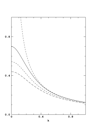
Fig. 3.3: The polarisation scalar, $\Pi(k)$, obtained from Eq. (3.72) using the solution of Eqs. (3.34) and (3.35) with $a=0.5$, is plotted for $\xi=0$: solid line; $\xi=0.5$; dashed line; $\xi=1.0$; dash-dot line. [The mass scale is fixed by setting $e^{2}=1$ .] The plot illustrates the deviation of the result from the perturbative one at small $k$. On the scale of this plot the fitting function of Eq. (3.76) lies exactly on top of the numerical results. The perturbative result of Eq. (3.17) is the short-dash line. [This figure is adapted from Burden et al. (1992a)]

The results can be summarised by the fit:

$$\Pi(k)=\frac{e^{2}}{8(k^{2}+e^{4}a^{2})^{\frac{1}{2}}}+be^{-c\frac{k^{2}}{e^{4}}}$$ (3.76)

with $\xi$ dependent fitting parameters $a$, $b$ and $c$ specified below, $(\xi,a,b,c)$:

$$(0.0,0.2044,8.760\times 10^{-2},7.767)~{},$$ (3.77)

$$(0.5,0.2541,5.055\times 10^{-2},11.70)~{},$$ (3.78)

$$(1.0,0.2778,-9.349\times 10^{-3},0.5285)~{}.$$ (3.79)

[Of course, in this calculation, a trivial multiplicative factor of $N_{f}$ appears on the right hand side of Eq. (3.76) if one uses $N_{f}$ fermions. A complicated dependence on $N_{f}$ can only arise when one carries out the simultaneous solution of Eqs. (3.34), (3.35) and (3.72). ]

The first thing one deduces from Eq. (3.76) is that the Ball-Chiu vertex, although yielding $\langle\overline{\psi}\psi\rangle$ essentially independent of the gauge parameter, $\xi$, it does entail Eq. (3.69); i.e., it does not lead to a gauge independent polarisation scalar. This is important and we will discuss it in some detail below in Sec. 3.7.

One observes from Eq. (3.76) and Fig. 3.3 that, at large $k^{2}$, the nonperturbative result returns to the perturbative one of Eq. (3.17). For small $k^{2}$, $\Pi(k)$ differs from the perturbative result which was used in the analyses described in the preceding subsections and predominantly in Pennington and Walsh (1991). The difference is a quantitative softening of the infrared behaviour of $\Pi(k)$ and it has been reported (Pennington and Walsh, 1991) that this has little effect on DCSB when used simply as input to Eqs. (3.34) and (3.35). The difference is not unimportant, however. Simply assuming that $\Pi(k)$ is bounded [in absolute value] and continuously differentiable on $(0,\infty)$ and that $\Pi(k)\sim 1/k$ for $k\rightarrow\infty$ is enough to ensure that, for large $r$, the potential associated with the dressed photon propagator is

$$V(r)=\frac{1}{1+\Pi(0)}\frac{e^{2}}{2\pi}\ln e^{2}r+\mbox{const.}+h(r)$$ (3.80)

where $h(r)$ falls off at least as fast as $1/r$ (Burden et al., 1992a). Hence, the large $r$ behaviour of the potential is dominated by a confining logarithmic term. It will be recalled that this was true of the bare photon propagator but not of the perturbatively dressed photon propagator. The inclusion of a dressed fermion-photon vertex and dressed fermion propagator [obtained with this vertex] at this level has thus restored the confining nature of QED₃  .

The first order response of the photon polarisation scalar to dynamical fermion mass generation is a modification on the small-$k^{2}$ domain which is just that domain relevant to DCSB. This may have an impact on the question of the existence of a critical number of flavours in QED₃ but a full analysis of the coupled fermion-photon DSE system with a physically reasonable vertex Ansatz would be the least necessary to address this. Preliminary results of such a project are described by Walsh (1990) but no firm conclusion may be drawn from this study.

3.7 Fermion-Photon Vertex and Gauge Invariance

The issue of gauge invariance in the DSE approach to the solution of gauge field theories is very important. Indeed, a manifest lack of gauge covariance in many works in this field has hindered its acceptance as an efficacious nonperturbative tool. [There are many contemporary works that still fail to address this issue.] We will discuss gauge covariance and invariance in the context of linear, covariant gauges which is the class of gauges in which most studies are undertaken.

The coupled fermion–gauge-boson DSE system is closed if the fermion–gauge-boson vertex is known. Further, it has become clear that, in Abelian theories, the fermion-gauge-boson vertex is crucial to ensuring the correct gauge parameter dependence of the objects one calculates in the DSE approach. This indicates the importance of this vertex in the DSE approach. This presents a problem, however, because, in Abelian gauge theories, the equation of which the vertex is the solution involves the kernel of the fermion-antifermion BSE which cannot be expressed in a closed form; i.e., the skeleton expansion of this kernel involves infinitely many terms. [The problem is even greater in non Abelian theories.]

As we have remarked, there have been no attempts to solve the DSE for the vertex. Instead, recognising the importance of the vertex, a number of authors have invested some effort into enumerating constraints that this vertex must satisfy and proposed Ansätze which satisfy them. The DSE for the fermion propagator and, in some cases, the coupled fermion-photon DSEs have then been solved using a given Ansatz.

There are six general constraints one can place on the fermion-gauge-boson vertex (Burden and Roberts, 1993):

(a)

It must satisfy the WTI;

(b)

It must be free of any kinematic singularities [i.e., expressing $\Gamma_{\mu}(p,q)$ as a function of $p$ and $q$ and a functional of the fermion propagator, $S(p)$, then $\Gamma_{\mu}$ should have a unique limit as $p^{2}\rightarrow q^{2}$];

(c)

It must reduce to the bare vertex in the free field limit in the manner prescribed by perturbation theory;

(d)

It must have the same transformation properties as the bare vertex, $\gamma_{\mu}$, under charge conjugation, $C$, and Lorentz transformations [such as $P$ and $T$, for example];

(e)

It should ensure local gauge covariance of the propagators and vertices; and

(f)

It should ensure multiplicative renormalisability of the DSE in which it appears.

Criterion (b) follows from Ball and Chiu (1980) and criterion (c) is related to this since together they are necessary to ensure that the vertex Ansatz has the correct perturbative limit. The charge conjugation element of criterion (d) is essential since it constrains the properties of $\Gamma_{\mu}(p,q)$ under $p\leftrightarrow q$.

Although condition (a) is a consequence of gauge invariance, it is only a statement about the longitudinal part of the vertex, and says nothing about the transverse part. By itself it is insufficient to ensure condition (e) (Burden and Roberts, 1991). A well defined set of transformation laws, which describe the response of the propagators and vertex in quantum electrodynamics to an arbitrary gauge transformation are given in papers by Landau and Khalatnikov (1956) and Fradkin (1956) [LKF] [see Appendix A]. These laws leave the DSEs and WTI form-invariant and one can, in principle, ensure condition (e) by choosing an Ansatz for $\Gamma$ which is covariant under the action of the LKF transformations. Unfortunately, however, the transformation rule for the vertex is quite complicated, making this procedure difficult to implement. Alternatively, since the LKF transformation rule for the fermion propagator and polarisation scalar are straightforward, one can use the LKF transformations to check a posteriori whether solutions for propagators obtained using a particular vertex Ansatz transform appropriately and hence whether the Ansatz used can possibly have been consistent with criterion (e).

The fermion-gauge-boson vertex in an Abelian gauge theory can be written in the form (Ball and Chiu, 1980):

$$\Gamma_{\mu}(p,q)=\Gamma_{\mu}^{\rm BC}(p,q)+\sum_{i=1}^{8}\;f^{i}(p^{2},q^{2},p\cdot q)\;T_{\mu}^{i}(p,q)~{},$$ (3.81)

where $\Gamma_{\mu}^{\rm BC}(p,q)$ is given in Eq. (3.5) and $T_{\mu}^{i}$ are the eight transverse tensors of Eq. (3.4) in Ball and Chiu (1980) of which those with $i=1,2,3$ are symmetric under $p\leftrightarrow q$ and the remainder are antisymmetric. The requirement (d) above implies that all of the $f^{i}$ are symmetric except for $f^{6}$ which is antisymmetric. All vertex Ansätze which satisfy the WTI can be written in this form.

Criteria (a)-(d) and (f) have been used (Curtis and Pennington, 1990) in an analysis of QED₄ to argue that a minimal admissible form of the vertex has $f^{i}\equiv 0\>\>\forall\;i\neq 6$ and $f^{6}$ chosen so as to yield Eq. (3.66).

Gauge Technique and DCSB.       This is an ideal point to remark that there is an approach to solving the DSEs that differs substantially in method to the studies described above: the “gauge technique” (GT) (Salam, 1963). This approach, based in Minkowski space, assumes that the elements of the DSE approach [i.e., the propagators and vertices] have spectral representations in terms of which the DSEs are reformulated and then solved for directly. For example, in the context of studies of DCSB, it is assumed that a spectral density, $\rho_{\psi}$, exists such that the fermion propagator can be written:

$$S(p)=\int_{-\infty}^{\infty}d\omega\,\frac{\rho_{\psi}(\omega)}{\not\!p-\omega}$$ (3.82)

and that the fermion–gauge-boson vertex has a similar form. In fact, a commonly used vertex Ansatz in this approach is (Delbourgo and West, 1977)

$$S(p)\Gamma_{\mu}^{\rm GT}(p,q)S(q)=\int_{-\infty}^{\infty}d\omega\,\rho_{\psi}(\omega)\frac{1}{\not\!p-\omega}\gamma_{\mu}\frac{1}{\not\!q-\omega}~{},$$ (3.83)

which has been used in an analysis of QED₃ (Waites and Delbourgo, 1992). For comparison it is useful to note that Eq. (3.83) corresponds, in Euclidean space, to the vertex

$$\Gamma_{\mu}^{\rm GT}(p,q) = i\left(\alpha_{\mu}S^{-1}(q)-S^{-1}(p)\alpha_{\mu}\right),$$ (3.84)

with $\alpha_{\mu}=[\gamma\cdot p\gamma_{\mu}+\gamma_{\mu}\gamma\cdot q]/[p^{2}-q^{2}]$, or alternatively:

$$i\Gamma_{\mu}^{\rm GT}(p,q)=\frac{p^{2}A(p)-q^{2}A(q)}{p^{2}-q^{2}}\,i\,\gamma_{\mu}+\frac{A(p)-A(q)}{p^{2}-q^{2}}\,i\,\gamma\cdot p\gamma_{\mu}\gamma\cdot q+\,\frac{B(p)-B(q)}{p^{2}-q^{2}}(\gamma\cdot p\gamma_{\mu}+\gamma_{\mu}\gamma\cdot q).$$ (3.85)

The vertex, $\Gamma_{\mu}^{\rm GT}$, is easily seen to satisfy criteria (a) to (d) and must therefore be of the form Eq. (3.81).

Inserting Eqs. (3.82) and (3.83) into the DSE for the fermion propagator one obtains a linear equation for the spectral density. This is a feature of the gauge technique: it can reduce the fermion DSE to a linear equation. In fact, in practice, Ansätze for the propagators and vertices are almost always chosen so that the DSEs under consideration are linear integral equations for the spectral density.

In a manner similar to that in which the Ball-Chiu Ansatz can be improved using criterion (f) it is also possible to improve Eq. (3.83) by adding a correction term which ensures that the fermion DSE is multiplicatively renormalisable in this approach (King, 1983) and ensures gauge covariance of the fermion propagator for small- and large-$p^{2}$ [but not for intermediate momenta].

A property of this approach which may prove undesirable, however, is that the equations for the Dirac-vector and -scalar parts of the spectral density decouple in the limit of zero Lagrangian- and renormalised-bare-mass. In this case one always has the chiral symmetry preserving solution

$$S^{\rm W}(p)=-i\gamma\cdot p\sigma_{V}^{\rm W}(p)$$ (3.86)

and, in addition, it is also probable that the equation admits a dynamical chiral symmetry breaking solution which would have the form

$$S^{\rm NG}(p)=-i\gamma\cdot p\sigma_{V}^{\rm W}(p)+\sigma_{S}^{\rm NG}(p).$$ (3.87)

Here the notation indicates the Weyl (W) and Nambu-Goldstone (NG) modes respectively. [This was the case, for example, in the phenomenological QCD studies of Haeri and Haeri (1991).] We remark that in Eq. (3.86) and Eq. (3.87) the vector part of the propagator is necessarily the same.

The fermion DSE is the stationary point equation for the effective action discussed in in Corwnall, Jackiw and Tomboulis (1974) which, evaluated at this stationary point is (Stam, 1985; see also Sec. 7.2):

$$V[S]=\int\frac{d^{\rm d}p}{(2\pi)^{\rm d}}\left[{\rm tr}\ln[1-\Sigma(p)S(p)]+\frac{1}{2}{\rm tr}[\Sigma(p)S(p)]\right].$$ (3.88)

One might measure the relative stability of these extremals by evaluating the difference $V[S^{\rm NG}]-V[S^{\rm W}]$. For an Abelian gauge theory with $N_{f}$ flavours of fermion one finds [for ${\rm d}=3$ or $4$ since we use $4$ component spinors] that

$$V[S^{\rm NG}]-V[S^{\rm W}]=2N_{f}\int\frac{d^{\rm d}p}{(2\pi)^{\rm d}}\ln\left[1+\frac{1}{p^{2}}\frac{\sigma_{S}^{2}(p)}{\sigma_{V}^{2}(p)}\right]>0,$$ (3.89)

since it is reasonable to assume that $\sigma_{S}$ and $\sigma_{V}$ are real for real Euclidean $p^{2}$. [Since the equation for $\sigma_{S}$ is homogeneous, this difference can, in fact, be made arbitrarily large: $\sigma_{S}\rightarrow\lambda\sigma_{S}$.] Hence, based on this effective action [which is the same as the auxiliary field effective action at the stationary point] one finds that the gauge technique cannot support dynamical chiral symmetry breaking (Burden and Roberts, 1993). This result is true of any approach in which the equations for the Dirac-vector and -scalar pieces of the fermion propagator decouple. [We note that an extension of the CJT effective action to include a functional dependence on the fermion-gauge-boson vertex may allow for DCSB even when the equations decouple (Haeri, 1993).]

Gauge Covariance in the Quenched Approximation.       Criterion (c) has an important consequence. The unrenormalised fermion DSE in QED₃ and QED₄ can be written

$$1=(i\gamma\cdot p+m)S(p)+e^{2}\int\frac{d^{\rm d}q}{(2\pi)^{\rm d}}D_{\mu\nu}(p-q)\gamma_{\mu}S(q)\Gamma_{\nu}(q,p)S(p).$$ (3.90)

If one works in the quenched approximation, Eq. (3.11), then since

$$\int d\Omega_{\rm d}\frac{1}{(p-q)^{2}}\left(({\rm d}-3)\,p\cdot q+2\frac{p\cdot(p-q)\,(p-q)\cdot q}{(p-q)^{2}}\right)\equiv 0$$ (3.91)

it follows that, in Landau gauge, Eq. (3.90) admits the free propagator solution

$$S(p)=\frac{1}{i\gamma\cdot p}$$ (3.92)

for any vertex that satisfies criterion (c). It follows directly from this that if a given vertex Ansatz is to satisfy the gauge covariance criterion, (e), then, for arbitrary $\xi$, the associated fermion DSE must have the LKF transform of the free field propagator as its solution [Eq. (A.2)].

We can elucidate this further by considering the massless fermion DSE in configuration space:

$$\delta^{\rm d}(x-y)=\gamma\cdot\partial^{x}S(x-y)+$$ (3.93)

$$\!\!\!\!\!\!\!\!\!\!\!\!\!\!\!\!e^{2}\int d^{\rm d}zd^{\rm d}x^{\prime}d^{\rm d}y^{\prime}\gamma_{\mu}\left(D_{\mu\nu}^{\rm T}(x-z)+\partial^{z}\partial^{z}\Delta(x-z)\right)S(x-x^{\prime})\Gamma_{\nu}(z;x^{\prime},y^{\prime})S(y^{\prime}-y)$$

where we have explicitly divided the gauge-boson propagator into the sum of a transverse, gauge independent piece, $D_{\mu\nu}^{\rm T}$, and longitudinal, gauge dependent piece, $\Delta$. Making use of the WTI

$$\partial_{\mu}\Gamma_{\mu}(z;x^{\prime},y^{\prime})=S^{-1}(z-y^{\prime})\delta^{\rm d}(x^{\prime}-z)-\delta^{\rm d}(z-y^{\prime})S^{-1}(x^{\prime}-z)$$ (3.94)

and the identity $\int_{x^{\prime}}\gamma\cdot\partial^{x}S(x,x^{\prime})S^{-1}(x^{\prime},z)=\gamma\cdot\partial^{x}\delta^{\rm d}(x-z)~{},$ one obtains the massless DSE in the following form:

$$\delta^{\rm d}(x-y) = \gamma\cdot\partial^{x}S(x-y)$$ (3.95)

$$- e^{2}\left\{\int d^{\rm d}z[\gamma\cdot\partial^{x}\Delta(x-z)]\delta^{\rm d}(x-z)-[\gamma\cdot\partial^{x}\Delta(x-y)]\right\}S(x-y)$$

$$+ e^{2}\int d^{\rm d}zd^{\rm d}x^{\prime}d^{\rm d}y^{\prime}\gamma_{\mu}D_{\mu\nu}^{\rm T}(x-z)S(x-x^{\prime})\Gamma_{\nu}(z;x^{\prime},y^{\prime})S(y^{\prime}-y).$$

Now it is clear by inspection that if

$$\int d^{\rm d}zd^{\rm d}x^{\prime}d^{\rm d}y^{\prime}\gamma_{\mu}D_{\mu\nu}^{\rm T}(x-z)S(x-x^{\prime})\Gamma_{\nu}(z;x^{\prime},y^{\prime})S(y^{\prime}-y)=0~{};$$ (3.96)

then Eq. (A.2), with $S(x;\xi=0)$ given in Eq. (A.10), is a solution of the massless DSE; i.e., it is a solution if the last term on the right hand side of Eq. (3.90) is identically zero in Landau gauge. [We remark that Eq. (3.91) is only relevant in quenched approximation: beyond quenched approximation the integrand is modified and the integral is nonzero so that, even given (c), the free propagator is not a solution and gauge covariance plus Eq. (3.95) doesn’t require Eq. (3.96).]

As we have seen, most studies of the DSEs are undertaken in momentum space and it is a simple matter to transcribe Eqs. (3.95) and (3.96). We see that the solution of the DSE is LKF covariant if

$$\int\frac{d^{\rm d}q}{(2\pi)^{\rm d}}\,D_{\mu\nu}^{\rm T}(p-q)\gamma_{\mu}S(q)\Gamma_{\nu}(q,p)=0,$$ (3.97)

where $D_{\mu\nu}^{\rm T}(k)=(\delta_{\mu\nu}-k_{\mu}k_{\nu}/k^{2})/k^{2}$ in the quenched theory, in which case the propagator satisfies:

$$1=i\gamma\cdot pS(p)+\xi e^{2}\int\frac{d^{\rm d}q}{(2\pi)^{\rm d}}\frac{i\gamma\cdot(p-q)}{(p-q)^{4}}\left[S(p)-S(q)\right]$$ (3.98)

in the covariant gauge fixing procedure.

Equation (3.97) provides a much needed additional constraint upon the vertex function which, while not a full implementation of criterion (e), is nevertheless a restriction on the form of the transverse part of the vertex:

(e^′) In the absence of dynamical chiral symmetry breaking; i.e., for $\sigma_{S}\equiv 0$, the vertex must be such that Eq. (3.97) is satisfied,

where $D_{\mu\nu}^{\rm T}(k)$ is the transverse part of the quenched photon propagator. This is a necessary condition which must be satisfied by any vertex Ansatz if it is to confer gauge covariance on the quenched QED₃ and QED₄ DSEs.

We can apply this check in the case of the Curtis-Pennington vertex, Eq. (3.64), for which the fermion DSE in QED₃ is, in the absence of DCSB,

$$A(p)-1=\frac{-e^{2}\xi}{4\pi^{2}p^{2}}\int_{0}^{\infty}dq\,\frac{1}{A(q)}\left(\frac{p^{2}A(p)-q^{2}A(q)}{p^{2}-q^{2}}-\frac{p^{2}A(p)+q^{2}A(q)}{2pq}\ln\left|\frac{p+q}{p-q}\right|\right),$$ (3.99)

in which the right hand side is clearly zero in Landau gauge. Hence this vertex, or at least that part of it which contributes to the DSE, has the form necessary to ensure gauge covariance of the chirally symmetric fermion propagator. [We remark that here an infrared regulator, $\lambda_{\rm IR}$, is used to define $d(k,p)$ in Eq. (3.67) when $B(k)\equiv\,0$ and the limit $\lambda_{\rm IR}\rightarrow 0$ taken before evaluating the integral because it is finite.]

It is possible to solve this equation analytically (Burden and Roberts, 1993). The solution, for $\xi>0$, is

$$\frac{1}{A(p)}=1-\frac{e^{2}\xi}{8\pi p}\arctan\left(\frac{8\pi p}{e^{2}\xi}\right),$$ (3.100)

as it should be since this corresponds to the LKF transform of the massless, free fermion propagator in QED₃ [see Appendix A].

The fermion DSE for QED₄ using the Curtis-Pennington vertex is given in Curtis and Pennington (1991) and can be written formally as

$$A(p)-1=\frac{\xi\alpha_{0}}{4\pi p^{2}}\int_{0}^{\infty}dq^{2}\left[\theta(p^{2}-q^{2})\frac{q^{2}}{p^{2}}+\theta(q^{2}-p^{2})\frac{p^{2}}{q^{2}}\frac{A(p)}{A(q)}\right].$$ (3.101)

In Curtis and Pennington (1991) this equation was solved by introducing an upper bound on the $q^{2}$ integral with the result $A_{\rm R}(p^{2};\xi)=A_{\rm R}(\mu^{2};\xi)(p^{2}/\mu^{2})^{\gamma}$, $\gamma=\alpha_{0}\xi/(4\pi)/[1+\alpha_{0}\xi/(8\pi)]$, which illustrates that Eq. (3.64) ensures multiplicative renormalisability of the chirally symmetric fermion DSE for all $p^{2}$. However, this solution only agrees with the LKF transform of the free propagator at O$(\xi$). This defect arises because a hard cutoff was used, which violates Poincaré invariance and generates a spurious term in the equation. A detailed discussion of this can be found in Dong, et al. (1994), where the actual solution is shown to be $A_{\rm R}(p^{2};\xi)=A_{\rm R}(\mu^{2};\xi)(p^{2}/\mu^{2})^{\nu}$ with $\nu=\alpha_{0}\xi/(4\pi)$, which agrees with the LKF transform at all $\xi$.

It is interesting to note that the Ball-Chiu vertex alone, Eq. (3.5), does not satisfy criterion (e’) (Burden and Roberts, 1993). This is also a defect of the minimal gauge-technique vertex, Eq. (3.84), however, the addition suggested by King (1983) goes some way to eliminating this problem.

4 Four-dimensional Quantum Electrodynamics

Many of the remarks made and studies described in Sec. 3 are directly relevant to QED₄ . In the absence of a Lagrangian bare mass for the electron, the action for QED₄ has the same chiral symmetry as massless QCD. This being the case, one of the main goals of DSE studies in QED₄ over the last twenty years has been to answer the question of whether there is a phase in which chiral symmetry is dynamically broken and, if so, what is the order of the phase transition. [As we will see, this is related to the question of whether QED₄ is trivial or not.] Naturally, the tool used to address this question is the DSE for the renormalised electron self energy in QED₄ which, in Euclidean space, is

$$\Sigma(p) = i\gamma\cdot p\,(Z_{1}-1)-(m-Z_{1}\,m_{0})+Z_{1}e^{2}\int\frac{d^{4}q}{(2\pi)^{4}}\Gamma_{\mu}(p,q)D_{\mu\nu}(p-q;\xi)S_{F}(q)\gamma_{\nu}~{};$$ (4.1)

a minor modification of Eq. (3.7) with significant consequences.

The first of these we have mentioned above. In Landau gauge and at O($e^{2}$) one has

$$Z_{1}\equiv\,1~{}.$$ (4.2)

This result has been used in many studies to simplify this equation. Further, it has been used as an approximation in many model DSE studies in QCD.

4.1 Dynamical Chiral Symmetry Breaking

The second consequence is of particular use in the rainbow, quenched approximation to QED₄ . In this approximation, it follows from Eq. (3.91) that the angular integral for the Dirac-vector component of the electron self-energy vanishes in Landau gauge so that, subject to Eq. (4.2), Eq. (4.1) admits the solution $A(p^{2})\equiv 1$ with $B(p^{2})$ obtained as the solution of the following nonlinear integral equation:

$$B(p^{2}) = m_{0}+(3+\xi)\,e^{2}\,\int^{\Lambda_{\rm UV}}\,\frac{d^{4}q}{(2\pi)^{4}}\,\frac{1}{(p-q)^{2}}\,\frac{B(q^{2})}{q^{2}+B^{2}(q^{2})}~{},$$ (4.3)

where $\Lambda_{\rm UV}$ is a cutoff which is necessary if $m_{0}\neq\,0$.

In addition, one may make use of the result:

$$\int\,d\Omega_{\rm 4}\,\frac{e^{2}}{(p-q)^{2}}=\theta(p^{2}-q^{2})\,\frac{e^{2}}{p^{2}}+\theta(q^{2}-p^{2})\,\frac{e^{2}}{q^{2}},$$ (4.4)

where $\int\,d\Omega_{\rm 4}\;\equiv\;\frac{1}{2\pi^{2}}\,\int_{0}^{\pi}\,d\beta\,\sin^{2}\beta\,\int_{0}^{\pi}\,d\theta\,\sin\theta\,\int_{0}^{2\pi}\,d\phi$, to reduce Eq. (4.3) to the following differential equation:

$$x\,B^{\prime\prime}(x)+2\,B^{\prime}(x)+\frac{3\alpha}{4\pi}\,\frac{B(x)}{x+B^{2}(x)}=0,$$ (4.5)

where $x=p^{2}$, with the boundary conditions

$$\lim_{x\rightarrow 0}\left(\frac{d}{dx}[x^{2}\,B(x)]\right)=0\;\; \;\;{\rm and}\;\; \;\;\lim_{x\rightarrow\Lambda^{2}_{\rm UV}}\left(\frac{d}{dx}[x\,B(x)]\right)=m_{0}~{}.$$ (4.6)

The problem of studying DCSB in the rainbow, quenched approximation to QED₄ is thus reduced to a study of this differential equation.

This is an opportune point to remark that Eq. (4.4) has been used as the basis for an extensively used approximation in phenomenological DSE studies of QCD and QED₄ beyond quenched approximation. Many authors have assumed that it is reasonable to write [i.e., the angle approximation]

$$\int\,d\Omega_{\rm 4}\,\frac{\alpha((p-q)^{2})}{(p-q)^{2}}\approx\theta(p^{2}-q^{2})\,\frac{\alpha(p^{2})}{p^{2}}+\theta(q^{2}-p^{2})\,\frac{\alpha(q^{2})}{q^{2}}~{},$$ (4.7)

with the function $\alpha(p^{2})$ assumed to be monotonically decreasing on $[0,\infty)$. This approximation has been critically analysed (Roberts and McKellar, 1990) and found to be reasonable only if $\alpha(0)$ is not large; i.e., of O($1$) or less.

Miransky Scaling.       Equation (4.5) has been studied by Fukuda and Kugo (1976) and the results have a direct analogue in those of Sec. 3.5. If one sets $m_{0}=0$ then Eq. (4.5) is obviously scale invariant. In this case the scale is set by choosing $B(0)=1$ and the solution then has the following power series expansion around $x=0$:

$$B(x)=1-\frac{3\alpha}{8\pi}\,x-\frac{\alpha}{64\pi}\,\left(\frac{3\alpha}{\pi}-8\right)\,x^{2}+\ldots~{}.$$ (4.8)

The asymptotic behaviour of the solution for large-$x$ is easily found to be

$$B(x)\sim\left\{\begin{array}[]{c}\displaystyle x^{-\frac{1}{2}+\frac{1}{2}\sqrt{1-3\alpha/\pi}},\;\;\alpha\leq\frac{\pi}{3}\\ \displaystyle\frac{1}{\sqrt{x}}\cos\left[\frac{1}{2}\sqrt{3\alpha/\pi-1}\,\ln\,x\right],\;\;\alpha\geq\frac{\pi}{3}\end{array}\right.~{}.$$ (4.9)

If one demands that the ultraviolet boundary condition of Eq. (4.6) be satisfied at some finite $\Lambda_{\rm UV}$ then it is clear that a nonzero solution for $B(p^{2})$ is admitted only if

$$\alpha>\alpha_{c}=\frac{\pi}{3}\;\;(\approx 1.047)$$ (4.10)

since the form of the solution valid for $\alpha<\alpha_{c}$ cannot satisfy this condition. In this case one has [see Sec. 3.5]

$$B(0)=\Lambda_{\rm UV}\,\exp\left(\,-\,\frac{\pi}{\sqrt{\alpha/\alpha_{c}-1}}+\delta\right)~{},$$ (4.11)

where $\delta$ is some phase, and the conclusion is that chiral symmetry may be dynamically broken in rainbow-quenched QED₄ if the coupling exceeds $\alpha_{c}$. A study of the stability of the nonzero solution for $B$, the solution which corresponds to a Nambu-Goldstone mode realisation of chiral symmetry, relative to the solution $B=0$, which corresponds to a realisation of chiral symmetry in the Wigner-Weyl mode, using the auxiliary field effective action (Roberts and Cahill, 1986) shows that the Nambu-Goldstone mode is indeed dynamically favoured for $\alpha>\alpha_{c}$.

As the critical coupling is approached, $B(0)$ and $\langle\overline{\psi}\psi\rangle$ are interchangeable as order parameters of DCSB. Equation (4.11) shows then that, in rainbow-quenched approximation, QED₄ has an infinite order phase transition. In models such as this one Eq. (4.11) is often referred to as “Miransky Scaling” (Miransky, 1985a).

It has been pointed out by Roberts and Cahill (1986), however, that in the limit $m_{0}=0$ the integral equation admits a solution even when the cutoff is removed; i.e., when $\Lambda_{\rm UV}=\infty$. In this case the ultraviolet boundary condition can be satisfied for any value of $\alpha$ and hence rainbow-quenched QED₄ admits DCSB for all values of the coupling. [See also, Atkinson and Johnson (1987).] This problem has also been studied using the vertex Ansatz of Eq. (3.64) (Curtis and Pennington, 1992); i.e., beyond rainbow approximation. In this case it is convenient to solve the integral equations directly because of the complicated structure of the vertex but the same result is obtained; i.e., a dynamical mass is generated for all values of the coupling.

In this light the existence of a critical coupling in massless QED₄ might be seen as the result of the imposition of a cutoff which can be viewed as an auxiliary condition, not intrinsic to the model, but relevant to the consideration of whether the model is a reasonable representation of QED₄ . For example, it might be argued that the appearance of the Landau ghost in perturbation theory suggests that the quenched approximation cannot possibly be valid at all momentum scales and hence that introducing a cutoff is a simple manner in which to model the effect of vacuum polarisation contributions.

However, dynamical chiral symmetry breaking in theories with ultraviolet divergences is a subtle problem (see, for example, Fomin et al., 1983, pp. 9-10 and pp. 64-65; Miransky, 1985a and 1985b). In a recent reanalysis of this problem (Curtis and Pennington, 1993) it is argued that dynamical chiral symmetry breaking in quenched QED₄ cannot be studied simply by setting $m_{0}=0$ in Eq. (4.1) and allowing the momentum integration to range over $[0,\infty)$ but rather that renormalisation plays an important role. The vertex Ansatz of Eq. (3.64), which ensures multiplicative renormalisability of the fermion DSE in QED₄ , is therefore well suited to this study. These authors suggest that in order to ensure conservation of the axial vector current in the renormalised theory, which can be interpreted as a definition of masslessness in the theory, one must take the cutoff to infinity and the bare mass to zero in such a way that their product approaches zero. This ensures that, since the bare composite operator $(\overline{\psi}\gamma_{5}\psi)_{\Lambda_{\rm UV}}$ depends on the cutoff,

$$\partial_{\mu}\,J^{5}_{\mu}=2\,m_{0}\,(\overline{\psi}\gamma_{5}\psi)_{\Lambda_{\rm UV}}=2\,(Z_{2}^{-1}\,m_{0})\,(\overline{\psi}\gamma_{5}\psi)_{\rm R}\;\stackrel{{\scriptstyle\Lambda_{\rm UV}\rightarrow\infty}}{{\rightarrow}}\;0~{},$$ (4.12)

where $Z_{2}$ is the mass renormalisation constant, and can be implemented through a definition of the renormalised theory with $m_{0}=0$ and with a cutoff $\Lambda_{\rm UV}<\infty$. In this way a Nambu-Goldstone realisation of chiral symmetry; i.e., DCSB, was found to be possible only for

$$\alpha>\alpha_{c}\approx 0.93$$ (4.13)

and Miransky scaling was observed at the critical coupling. This result was only weakly dependent on the gauge parameter, a result that one can attribute to the efficacy of the vertex Ansatz [see Sec. 3.7].

Mean Field Scaling - Vacuum Polarisation Ansatz.       A question that arises is whether the existence and order of the phase transition in QED₄ is sensitive to the nature of the approximations. The studies described above suggest that going beyond rainbow approximation does not qualitatively affect the results but what is the effect of the quenched approximation? Given the results discussed in Sec. 3.5 it is clear that going beyond quenched approximation can introduce another dimensionless parameter into the theory, the number of electrically active fermions, with respect to which there may exist critical behaviour. A number of authors have addressed these questions.

The first step is to choose a form for the vacuum polarisation. Motivated by the large-$k^{2}$ form of the vacuum polarisation in perturbation theory at one loop order, the usual choice is

$$\omega(k^{2})\equiv 1+\Pi(k^{2})=1+\frac{N_{f}\,\alpha}{3\pi}\,\ln\left[\frac{\Lambda_{\rm UV}^{2}}{k^{2}+\mu^{2}}\right]$$ (4.14)

where $N_{f}$ is the number of active fermions and $\mu^{2}$ is an infrared regulator. In some studies $\mu^{2}$ is set to $0$ (Kondo, 1990; Gusynin, 1990; Kondo, 1992; Kondo and Nakatani, 1992b; Maris, 1993, Sec. 4.3) while in others it is related to $B(0)$, e.g., $\mu^{2}=B(0)^{2}$ (Oliensis and Johnson, 1990), in order to incorporate some information from the fermion DSE in the expression for the vacuum polarisation. In any event it has little effect on the results. [Equation (4.14) can be obtained from Eq. (3.14) with ${\rm d}=3\rightarrow\,4$ using bare fermion propagators and a bare fermion-photon vertex.] Such a form has been used in almost all studies to date in concert with the approximation of Eq. (4.7) in which case one obtains $A(p^{2})\equiv\,1$ and the following differential equation for $B(x=p^{2})$:

$$x\,B^{\prime\prime}(x)+B^{\prime}(x)\,\left[1+\frac{\omega+\omega^{\prime}}{\omega}\ \left(1+\frac{\omega^{\prime}}{\omega+\omega^{\prime}}-\frac{\omega\,[\omega^{\prime}+\omega^{\prime\prime}]}{[\omega+\omega^{\prime}]^{2}}\right)\right]+\,\frac{3\alpha}{4\pi}\,\frac{\omega+\omega^{\prime}}{\omega^{2}}\,\frac{B(x)}{x+B(x)^{2}}=0~{},$$ (4.15)

where $\omega^{\prime}$ and $\omega^{\prime\prime}$ represent derivatives of $\omega$ with respect to the variable $t=\ln\,x$, with boundary conditions

$$\left[x^{2}\,B^{\prime}(x)\right]_{x=0}=0\;\; \;\;{\rm and}\;\; \left[(\omega^{\prime}+\omega)\,B(x)+\omega\,x\,B^{\prime}(x)\right]_{x=\Lambda^{2}_{\rm UV}}=0~{}.$$ (4.16)

This differential equation can be solved numerically (Oliensis and Johnson, 1990) and one finds that, with $N_{f}=1$, it admits a nonzero solution for

$$\alpha>\alpha_{c}\approx 2.00$$ (4.17)

and that the phase transition is of finite order. Further analysis (Kondo, 1990; Gusynin, 1990; Kondo, 1992; Kondo and Nakatani, 1992b; Maris, 1993, Sec. 4.3) shows that in this case, in contrast to Eq. (4.11),

$$B(0)\sim\Lambda_{\rm UV}\,\left(\alpha-\alpha_{c}\right)^{\frac{1}{2}}~{};$$ (4.18)

i.e., one has a second order phase transition with the classical mean field value for the critical exponent. Both $\langle\overline{\psi}\psi\rangle$ and $B(0)$ behave in the same way near the critical coupling (Kondo and Nakatani, 1992b).

It is obvious (Kondo and Nakatani, 1992b; Maris, 1993, Sec. 4.3) that if Eq. (4.7) is not used in order to obtain an approximate differential equation but instead Eq. (4.14) is used directly in the integral equation form of the fermion DSE in QED₄ , then one encounters a problem with the Landau ghost: the kernel of the integral equation, which involves

$$1+\Pi(k^{2}+p^{2}-2\,k\,p\,\cos\theta)$$ (4.19)

where the argument of $\Pi$ can attain a maximum value of $4\,\Lambda_{\rm UV}^{2}$, has a nonintegrable divergence unless

$$\alpha\,N_{f}\,<\frac{3\,\pi}{2\,\ln 2}\approx\,6.80$$ (4.20)

which restricts the number of flavours that one may consider. A first estimate based on Eq. (4.17) is that Eq. (4.14) will not be a viable Ansatz for $N_{f}>3$.

Numerical studies of the coupled integral equations for $A(p^{2})$ and $B(p^{2})$ using Eq. (4.14) in rainbow approximation (Kondo and Nakatani, 1992b; Maris, 1993, Sec. 4.3) find nontrivial solutions only for $N_{f}=1,2$ with critical couplings (Maris, 1993, Sec. 4.3)

$$\alpha_{c}(N_{f}=1)\approx 2.07\;\; \;\;{\rm and}\;\; \alpha_{c}(N_{f}=2)\approx 2.82~{}.$$ (4.21)

Kondo and Nakatani (1992b) used an Ansatz for the vacuum polarisation that differs slightly from Eq. (4.14), one which reflects the possible regularisation ambiguities, and in this case the value of the critical coupling depends on the choice of the additional parameters. Indeed, it is possible to choose the additional parameters and the number of active fermions, $N_{f}^{C}$, such that one does not have DCSB irrespective of the strength of the coupling. Avoiding such a complication, the numerical solution of the coupled integral equations leads to the same mean field scaling behaviour as the approximate differential equation.

Mean Field Scaling - Solving for the Vacuum Polarisation.       Given these last remarks, an obvious improvement would be to solve the coupled fermion and photon DSEs in Landau gauge using rainbow approximation:

$$A(p^{2})=1$$

$$+ \alpha_{0}\,\int_{0}^{\Lambda^{2}_{\rm UV}}\,\frac{dk^{2}\,k^{2}}{4\pi}\,\frac{A(k^{2})}{k^{2}\,A(k^{2})^{2}+B(k^{2})^{2}}\int_{0}^{\pi}\,\frac{d\theta}{\pi}\,2\,\sin^{2}\theta\,\frac{k\,\left[3\,(k-p)^{2}\,\cos\theta-2\,k\,p\,\sin^{2}\theta\right]}{p\,(k-p)^{4}\,[1+\Pi((k-p)^{2})]}~{},$$

$$B(p^{2}) = \!\!m_{0}+\!\!\alpha_{0}\,\int_{0}^{\Lambda^{2}_{\rm UV}}\,\frac{dk^{2}\,k^{2}}{4\pi}\,\frac{B(k^{2})}{k^{2}\,A(k^{2})^{2}+B(k^{2})^{2}}\int_{0}^{\pi}\,\frac{d\theta}{\pi}\,2\,\sin^{2}\theta\,\frac{3}{(k-p)^{2}\,[1+\Pi((k-p)^{2})]},$$ (4.23)

$$\Pi(p^{2}) = -\,\frac{4}{3}\,\alpha_{0}\,N_{f}\,\int_{0}^{\Lambda^{2}_{\rm UV}}\,\frac{dk^{2}\,k^{2}}{4\pi}\,\int_{0}^{\pi}\,\frac{d\theta}{\pi}\,2\,\sin^{2}\theta\,\frac{A(k_{+}^{2})\,A(k_{-}^{2})\,\left(\frac{k^{2}}{p^{2}}\,[8\,\cos^{2}\theta-2]-\frac{3}{2}\right)}{[k_{+}^{2}A(k_{+}^{2})^{2}+B(k_{+}^{2})^{2}]\,[k_{-}^{2}A(k_{-}^{2})^{2}+B(k_{-}^{2})^{2}]}$$ (4.24)

where $\alpha_{0}$ is the bare coupling, $m_{0}$ is the bare electron mass and $k_{\pm}^{2}=k^{2}+\mbox{\small$\frac{1}{4}$}p^{2}\pm\,k\,p\,\cos\theta$. Such a study has been undertaken by Rakow (1991).

The main body of the study concentrates on $N_{f}=1$ and it is assumed that $Z_{1}\equiv 1$, Eq. (4.2), while

$$Z_{2}\equiv\frac{1}{A(0)}\;\; {\rm and}\;\; \;\;Z_{3}\equiv\frac{1}{1+\Pi(0)}~{},$$ (4.25)

which follows from $S^{f}=Z^{f}_{2}\tilde{S}^{f}$, $D_{\mu\nu}=Z_{3}\tilde{D}_{\mu\nu}$ and Eq. (2.34) in Sec. 2.3, with renormalisation at $p^{2}=0$ rather than on the mass shell. Clearly, deviations from $A(p^{2})\equiv\,1$ measure the violation of the Ward Identity in rainbow approximation, Eq. (2.32). The results are then analysed in terms of a renormalised mass and coupling:

$$m_{\rm R}=\frac{B(0)}{A(0)}=Z_{2}\,B(0)\; \;\;{\rm and}\;\; \alpha_{\rm R}={\alpha_{0}\over A(0)^{2}\,[1+\Pi(0)]}=Z_{2}^{2}\,Z_{3}\,\alpha_{0}~{},$$ (4.26)

respectively, with $\alpha_{\rm R}$ measuring the effect of charge screening due to fermion loops.

It is found that with $m_{0}=0$ and for $N_{f}=1$ there is a critical coupling

$$\alpha_{c}\approx 2.25$$ (4.27)

such that

$$\langle\overline{\psi}\psi\rangle_{\Lambda_{\rm UV}}=\Lambda^{3}_{\rm UV}\,\left(\alpha_{0}-\alpha_{c}\right)^{\frac{1}{2}}~{};$$ (4.28)

i.e., that one has mean field scaling behaviour in the model, but that the critical exponent approaches the mean field value of $\frac{1}{2}$ very slowly. [See Creswick et al. (1992) for a pedagogical discussion of phase transitions and renormalisation group methods in physics.] It has been shown that

$$\mbox{$\langle\overline{\psi}\psi\rangle$\ }\sim\Lambda^{2}_{\rm UV}\,m_{\rm R}$$ (4.29)

and hence, identifying $\alpha_{0}$ as $\alpha(\Lambda_{\rm UV})$, Eq. (4.28) leads to the following $\beta$-function:

$$\beta(\alpha)\equiv\Lambda_{\rm UV}\,\frac{\partial}{\partial\Lambda_{\rm UV}}\ln\,\alpha(\Lambda_{\rm UV})=\,-2\left[\alpha(\Lambda_{\rm UV})-\alpha_{c}\right]$$ (4.30)

which suggests that unquenched, rainbow approximation QED₄ has an ultraviolet stable fixed point at $\alpha_{0}=\alpha_{c}$; a result supported by lattice simulations (Kogut et al., 1988a, 1988b).

In the limit $\alpha_{0}\rightarrow\alpha_{c}$ from above it is found that $\alpha_{\rm R}\rightarrow 0$ logarithmically; i.e., recall that $m_{\rm R}$ vanishes as $\alpha_{0}\rightarrow\alpha_{c}$,

$$\alpha_{\rm R}\propto\,-\,\frac{1}{\ln\,m_{\rm R}}\propto\frac{1}{\ln\xi}$$ (4.31)

where $\xi=\Lambda_{\rm UV}/m_{\rm R}$ is the correlation length in QED₄ . The continuum limit of the theory is defined as the limit $\xi\rightarrow\infty$. It follows from Eq. (4.31) that the continuum limit of unquenched, rainbow approximation QED₄ is trivial in the sense that it does not involve photons interacting with charged fermions, since it is not possible to obtain an infinite correlation length at nonzero coupling.

It is clear from these observations that solving for the vacuum polarisation yields the same results as the Ansatz of Eq. (4.14) with only minor quantitative differences. The problem of the “Landau-ghost” is not removed by a simultaneous solution of the fermion and photon DSEs in rainbow approximation.

Interacting Continuum Limit?      The existence of a phase in which chiral symmetry is dynamically broken suggests that at strong coupling [$\alpha_{0}\geq\alpha_{c}$] in QED₄ there are Goldstone modes; i.e., massless, pseudoscalar $e^{+}$-$e^{-}$ bound states. In this connection, one notes that in addition to studying the DSEs for the fermion and photon propagators in rainbow approximation, Rakow (1991) solved the following approximate form of the integral equations for the pseudoscalar and scalar electron-positron scattering amplitudes:

$$S_{5}(p^{2},r^{2})=\alpha_{0}\,\int_{0}^{\pi}\,\frac{d\theta}{\pi}\,2\,\sin^{2}\theta\frac{3\pi}{t^{2}\,[1+\Pi(t^{2})]}$$

$$+\alpha_{0}\,\int_{0}^{\Lambda^{2}_{\rm UV}}\,\frac{dk^{2}\,k^{2}}{4\pi}\,\frac{S_{5}(k^{2},r^{2})}{k^{2}\,A(k^{2})^{2}+B(k^{2})^{2}}\int_{0}^{\pi}\,\frac{d\theta}{\pi}\,2\,\sin^{2}\theta\frac{3}{q^{2}\,[1+\Pi(q^{2})]}~{},$$

$$S_{1}(p^{2},r^{2})=\alpha_{0}\,\int_{0}^{\pi}\,\frac{d\theta}{\pi}\,2\,\sin^{2}\theta\frac{3\pi}{t^{2}\,[1+\Pi(t^{2})]}$$

$$+\alpha_{0}\,\int_{0}^{\Lambda^{2}_{\rm UV}}\,\frac{dk^{2}\,k^{2}}{4\pi}\,S_{1}(k^{2},r^{2})\,\frac{k^{2}A(k^{2})^{2}-B(k^{2})^{2}}{[k^{2}\,A(k^{2})^{2}+B(k^{2})^{2}]^{2}}\int_{0}^{\pi}\,\frac{d\theta}{\pi}\,2\,\sin^{2}\theta\frac{3}{q^{2}\,[1+\Pi(q^{2})]}$$

where $\;t^{2}=p^{2}+r^{2}-2\,p\,r\,\cos\theta\;$ and $\;q^{2}=k^{2}+p^{2}-2\,k\,p\,\cos\theta$. These equations have been averaged over $p\cdot r$ and describe $[\psi(p);\overline{\psi}(-p)]$$\rightarrow$ $[\psi(r);\overline{\psi}(-r)]$ scattering.

In studying the solution of these equations it was observed that, at fixed values of $\alpha_{\rm R}$, these amplitudes did not scale; i.e., there was a dependence on $p/m_{\rm R}$. Indeed, the pseudoscalar amplitude manifested a contribution that diverged in the limit $m_{0}\rightarrow\,0$ obviously as a result of the formation of the Goldstone mode. This lack of scaling at constant $\alpha_{\rm R}$ suggests that another operator is relevant in the continuum limit.

The fact that another operator is relevant in the continuum limit can also be inferred from Eq. (4.9). In the absence of interactions the mass operator, $\overline{\psi}\psi$, diverges as $\Lambda^{2}_{\rm UV}$:

$$\overline{\psi}\psi\sim\int^{\Lambda^{2}_{\rm UV}}\,ds\,s\,{\rm tr}\,[S(p)]\;\stackrel{{\scriptstyle\Lambda^{2}_{\rm UV}\rightarrow\infty}}{{\propto}}\;\Lambda^{2}_{\rm UV}~{}.$$ (4.35)

In the interacting case, using Eq. (4.9), it diverges as $\Lambda_{\rm UV}^{1+\surd[1-3\alpha/\pi]}$ from which one can infer that its interaction-induced anomalous dimension is

$$\gamma_{\overline{\psi}\psi}=\sqrt{1-\frac{3\alpha}{\pi}}-1,$$ (4.36)

in quenched approximation and hence that the net dimension of the operator is

$$d_{\overline{\psi}\psi}=2+\sqrt{1-\frac{3\alpha}{\pi}}~{}.$$ (4.37)

In quenched, rainbow approximation [also called the planar approximation] the dimension of $[\overline{\psi}\psi]^{2}$ is just $2\,d_{\overline{\psi}\psi}$ and one is therefore lead to infer that, in the continuum limit [obtained, in this approximation, as $\alpha\rightarrow\,\frac{\pi}{3}$] $d_{[\overline{\psi}\psi]^{2}}\rightarrow\,4$ and hence that it becomes a relevant operator. This inference is supported by an analysis of quenched QED₄ which goes beyond the rainbow approximation, using the dressed electron-photon vertex of Eq. (3.64) (Atkinson et al., 1993).

Rakow (1991) studied QED₄ with the additional chirally-invariant, four-fermion interaction term

$$\int\,d^{4}x\,\frac{G_{0}}{2}\,\left[\overline{\psi}(x)\psi(x)\overline{\psi}(x)\psi(x)-\overline{\psi}(x)\gamma_{5}\psi(x)\overline{\psi}(x)\gamma_{5}\psi(x)\right]$$ (4.38)

which is just the interaction of the Nambu–Jona-Lasinio model [NJLM] (Nambu and Jona-Lasinio, 1961). With this term, Eqs. (4.23) and (4.1) receive the additive corrections:

$$\frac{G_{0}}{\pi}\,\int_{0}^{\Lambda^{2}_{\rm UV}}\,\frac{dk^{2}\,k^{2}}{4\pi}\,\frac{B(k^{2})}{k^{2}\,A(k^{2})^{2}+B(k^{2})^{2}}\; \;\;{\rm and}\;\; \;G_{0}\,+\,\int_{0}^{\Lambda^{2}_{\rm UV}}\,\frac{dk^{2}\,k^{2}}{4\pi}\,\frac{S_{5}(k^{2},r^{2})}{k^{2}\,A(k^{2})^{2}+B(k^{2})^{2}}~{},$$ (4.39)

respectively, and the other equations remain unchanged. [This model was first considered by Leung et al. (1986).] With this additional interaction, Eq. (4.38), all of the functions scale with $p/m_{\rm R}$, the fermion and photon propagators and the pseudoscalar and scalar scattering amplitudes, showing that all of the interactions that are relevant in the continuum limit are now included.

With $\alpha_{0}=0$ one simply has the NJLM in which chiral symmetry is dynamically broken for $G_{0}\Lambda^{2}_{\rm UV}\geq 4\pi^{2}$. In general the model has a two-dimensional phase diagram in the $(G_{0}\Lambda^{2}_{\rm UV},\alpha_{0})$-plane. From Fig. 14 of Rakow (1991) one infers that the model has DCSB on a set which, in the first quadrant, can be represented approximately as:

$${\cal S}_{1}=\left\{(G_{0}\Lambda^{2}_{\rm UV},\alpha_{0})\,:\;G_{0}\Lambda^{2}_{\rm UV}\geq 0,\;\alpha_{0}\geq 0,\;\frac{G_{0}\Lambda^{2}_{\rm UV}}{4\pi^{2}}+\frac{\alpha_{0}}{\alpha_{c}}\geq 1\right\}~{}.$$ (4.40)

This is only a part of the picture, however, and for a given value of $\alpha_{0}\in[0,\infty)$ there is always a value of $G_{0}=G_{0}^{c}\in\,(-\infty,4\pi^{2}]$ such that the model exhibits DCSB for $G_{0}>G_{0}^{c}$: as $\alpha_{0}$ is increased $G_{0}^{c}$ moves towards $-\infty$. The domain in the $(G_{0}\Lambda^{2}_{\rm UV},\alpha_{0})$-plane on which chiral symmetry is dynamically broken is similar to that found in quenched, rainbow approximation (Leung et al., 1986).

One may now return to the question of triviality.

One notes that, for a given value of $\alpha_{\rm R}$, the correlation length increases as $G_{0}$ decreases and takes its maximum value at $G_{0}=\,-\infty$ but that at any point not on the phase boundary this maximum value is finite. On the phase boundary the renormalised coupling is always zero and hence, even with the four-fermion interaction of Eq. (4.38), the theory doesn’t have a continuum limit of interacting fermions.

There is another possibility, however. There has been speculation for some time (Miransky, 1985a; Kogut et al., 1988a, 1988b) that QED₄ has an interesting continuum limit of interacting, strongly-bound $e^{+}$-$e^{-}$ states. One can convince oneself of this possibility simply by looking at the effective action for QED₄ as obtained in Roberts and Cahill (1986), for example. Expanding this action, following the procedure of Roberts et al. (1988), for example, one finds interactions between the $e^{+}$-$e^{-}$ bound states whose strength is characterised by

$$g_{\rm Y}=\frac{{\rm const.}<\infty}{f}$$ (4.41)

where

$$f^{2}=\frac{1}{2\pi^{2}}\,\int_{0}^{\Lambda^{2}_{\rm UV}}\,ds\,s\,B(s)\,\frac{B(s)-\frac{1}{2}\,s\,B^{\prime}(s)}{(s+B(s)^{2})^{2}}~{}.$$ (4.42)

It is clear then that as one takes the cutoff to infinity, in order to recover the continuum limit, the theory will be one of interacting bosons if $f<\infty$ and free bosons if it is not.

It is quite clear from Eq. (4.9) that in quenched approximation $f$ is indeed finite. In going beyond quenched approximation, however, one must use numerical solutions, or some approximation to them, in which case one finds that $f=\infty$ (Gusynin, 1990; Kondo, 1990; Maris 1993); a result which suggests that the continuum limit is one of noninteracting bosons.

4.2 Analytic Structure of the Electron Propagator

The differential equation, Eq. (4.5), has been studied by Atkinson and Blatt (1979). This study revealed a “pathology” of the ladder approximation, used in all of the studies discussed in the previous section [except Kondo (1992)], that has recently attracted a good deal of attention. Solving Eq. (4.5) one finds that instead of an electron propagator with a real branch cut on the timelike $p^{2}$ axis, as expected on physical grounds, the electron propagator in rainbow-quenched QED₄ has a pair of complex conjugate branch points in the complex $p^{2}$ plane whose position depends on $\alpha$. The recent studies of rainbow approximation model DSEs for QCD (Stainsby and Cahill, 1990; Maris and Holties, 1992; Stainsby and Cahill, 1992; Stainsby, 1993; Maris, 1993) suggest that this pathology is an artifact of the rainbow approximation; a conclusion supported by the extended analysis of rainbow approximation QED₄ by Maris (1993, Sec. 4) whose analysis also suggests that this “pathology” survives the inclusion of the one-loop vacuum polarisation, itself calculated in rainbow approximation.

It may be that the resolution of this problem lies simply in using a dressed fermion-gauge boson vertex; the possibilities and constraints on which we discussed in Sec. 3.7. However, there have been no studies to date that test this hypothesis directly in QED₄ . It should be noted, however, that, in a QCD-based model, Burden et al. (1992b) demonstrated that the structure of the vertex does significantly affect the singularity structure of the fermion propagator.

In Sec. 3.7 we briefly discussed the gauge technique. This has also been applied to QED₄ by Delbourgo and West (1977) who advocate an iterative solution of the DSEs for the spectral densities.

At lowest order, as it is defined in this approach, the only equation of interest is

$$Z_{2}^{-1}=(\mbox{$\not\!p$}-m_{0})\,S^{(0)}(p)-ie^{2}\,\int\frac{d^{4}q}{(2\pi)^{4}}\,S^{(0)}(p)\,\Gamma^{(0)}_{\mu}(p,p-q)\,S^{(0)}(p-q)\,D^{\mu\nu(0)}(q)\,\gamma_{\nu}$$ (4.43)

where $S^{(0)}$ is given by the expression in Eq. (3.82), $\Gamma^{(0)}$ by Eq. (3.83) and

$$D^{\mu\nu(0)}(q)=\left(-g^{\mu\nu}+(1-\xi)\frac{q^{\mu}q^{\nu}}{q^{2}}\right){1\over q^{2}}$$ (4.44)

with $\xi$ the gauge parameter.

Making use of these definitions Eq. (4.43) becomes

$$Z_{2}^{-1}=\int_{-\infty}^{\infty}d\omega\,\frac{\rho_{\psi}(\omega)}{\not\!p-\omega}\left(\mbox{$\not\!p$}-m_{0}+\Sigma(p,\omega)\right)$$ (4.45)

with $\Sigma(p,\omega)$ obtained in the lowest order of perturbation theory:

$${\rm Im}\,\Sigma(p,\omega)=\frac{e^{2}\,(p^{2}-\omega^{2})}{16\,\pi\,p^{3}}\left[\xi\,(p^{2}+\omega^{2})-(\xi+3)\,p\,\omega\right]~{}.$$ (4.46)

Making use of the definitions

$$Z_{2}^{-1}=\int_{-\infty}^{\infty}d\omega\,\rho_{\psi}(\omega)\;\; \;\;{\rm and}\;\; m_{0}=Z_{2}\int_{-\infty}^{\infty}d\omega\,\omega\,\rho_{\psi}(\omega)$$ (4.47)

then Eq. (4.45) yields the following result in Landau gauge:

$$S^{(0)}(p)=\frac{1}{\mbox{$\not\!p$}-m}$$

$$-\left(\frac{m^{2}}{\mu^{2}}\right)^{2\eta}\,\Gamma(1-\eta)^{2}\,\Gamma(1+2\xi)\,\left[\frac{\mbox{$\not\!p$}}{p^{2}}\left[F\left(1-\eta,1-\eta;1;\frac{p^{2}}{m^{2}}\right)-1\right]+\frac{1-\eta}{m}\,F\left(1-\eta,2-\eta;2;\frac{p^{2}}{m^{2}}\right)\right]$$

where $\mu^{2}$ is an infrared cutoff and $\eta=-3\alpha/(4\pi)$. The next iteration in the procedure uses this result coupled with Eq. (3.83) and Eq. (4.44) in the DSEs for the photon propagator and electron-photon vertex.

The interesting feature of Eq. (4.2) is that the fermion propagator has a branch cut at $p^{2}=m^{2}$; i.e., it has the singularity structure expected on physical grounds. This is a feature that it has in common with the propagator obtained with the solution of a linearised form of Eq. (4.5) (Maris, 1993, Sec. 4.2):

$$x\,(x+m^{2})\,B^{\prime\prime}(x)+2\,(x+m^{2})\,B^{\prime}(x)+\frac{3\alpha}{4\pi}\,B(x)=0~{},$$ (4.49)

with $m\equiv B(0)$, which is a hypergeometric differential equation whose solution is

$$B(x)=m\,F\left(\frac{1}{2}+\frac{1}{2}\sqrt{1-\frac{3\alpha}{\pi}}\,,\,\frac{1}{2}-\frac{1}{2}\sqrt{1-\frac{3\alpha}{\pi}}\,;\,2\,;\,-\,\frac{x}{m^{2}}\right)~{}.$$ (4.50)

This is, perhaps, not surprising since the operational procedure in the gauge-technique is to ensure that one has linear equations in the spectral density. The study by Maris (1993, Sec. 4.2.3) emphasises that the singularity structure of the solution of the nonlinear differential equation is quite different from that of the solution of the linearised equation: it has complex conjugate branch points.

The application of the gauge technique to QED₄ has not been pursued further. It is not known whether the procedure, outlined briefly here, converges nor whether the desirable singularity structure of Eq. (4.2) survives further iteration. Given the results of Stainsby and Cahill (1990), Maris and Holties (1992), Stainsby and Cahill (1992), Stainsby (1993, Sec. 3) and Maris (1993, Sec. 4) it would be interesting to answer these questions. In addition to the limitations mentioned in Sec. 3.7, however, one must add that the procedure advocated is quite difficult to implement.

At present, in the study of Abelian gauge theories the ingredients that are necessary and/or sufficient to ensure physical singularity structure in the propagators remain unknown.

5 Gauge Boson Sector of QCD

We have briefly discussed the DSEs for QCD in Sec. 2.2 with the equation for the vacuum polarisation and gluon propagator represented diagrammatically in Fig. 2.5. In this section we will review the attempts that have been made to solve these equations, the approximations used and the results obtained. [See also, Hädicke (1991).] This is important because in the application of DSEs to hadronic physics a physically reasonable form for the quark propagator is needed and, in practice, this is obtained by solving the quark DSE with Ansätze for the gluon propagator and quark-gluon vertex, with the former often being motivated by studies of the DSE for the gluon propagator.

Before proceeding, however, this is an opportune point to make a number of observations. We use our Euclidean space conventions throughout this section, see Sec. 2.3.

In an arbitrary covariant gauge, specified by $\xi$, the gluon propagator can be written as

$$D_{\mu\nu}(q)=\left\{\delta_{\mu\nu}-\frac{q_{\mu}q_{\nu}}{q^{2}}\right\}\frac{1}{q^{2}[1+\Pi(q^{2})]}+\xi\frac{q_{\mu}q_{\nu}}{q^{4}}$$ (5.1)

where, as usual, $\Pi(q^{2})$ is the vacuum polarisation. It will be observed that only the transverse piece of the gluon propagator is modified by interactions. This is a result of BRS invariance which yields, in the covariant gauge fixing scheme, the STI (Pascual and Tarrach, 1984, pp. 42-45)

$$q_{\mu}\,D_{\mu\nu}(q)=\xi\frac{q_{\nu}}{q^{2}}~{}.$$ (5.2)

This is an important constraint.

The least ambiguity and/or uncertainty exists in the form of the gluon propagator at large spacelike-$q^{2}$ since this is the domain on which perturbation theory and the renormalisation group can be easily applied. Indeed, the evaluation of the asymptotic form of $\Pi(q^{2})$ is a textbook exercise (for example, Pascual and Tarrach, 1984, pp. 70-76). Determining the form of the propagator at smaller spacelike-$q^{2}$ is, however, a difficult problem.

In this connection, one can employ the renormalisation group in QCD to obtain an approximate relation between the vacuum polarisation and the running coupling constant in QCD. In Landau gauge, the renormalisation group equation for

$$\Delta(q^{2};\alpha_{0})\equiv\frac{\alpha_{0}}{1+\Pi(q^{2};\alpha_{0})}$$ (5.3)

is, with $Z_{\Delta}=(Z_{1}^{gh})^{-2}\,(Z_{3}^{gh})^{2}$ where $Z_{1}^{gh}$ and $Z_{3}^{gh}$ are renormalisation constants for the ghost-gluon vertex and ghost wave function, respectively,

$$\left[\mu\,\frac{\partial}{\partial\mu}+\beta(\alpha(\mu))\,\alpha(\mu)\,\frac{\partial}{\partial\alpha}-\mu\,\frac{d}{d\mu}\ln\,Z_{\Delta}\,\right]\,\Delta_{\rm R}(q^{2};\alpha(\mu))=0$$ (5.4)

where $\beta(\alpha)$ is the QCD $\beta$-function:

$$\beta(\alpha(\mu))=\frac{\alpha(\mu)}{\pi}\,\frac{2\,N_{f}-33}{6}+{\rm O}((\alpha(\mu)/\pi)^{2})~{}.$$ (5.5)

If one assumes that

$$Z_{1}^{gh}=Z_{3}^{gh}~{},$$ (5.6)

which is sometimes called the “Abelian approximation”, then the last term on the left-hand-side of Eq. (5.4) vanishes and $\Delta_{R}$ satisfies the same renormalisation group equation as $\alpha_{\rm R}$. Since at large spacelike momenta one has $\Delta(q^{2}\rightarrow\infty)=\alpha$ then the equivalence of the renormalisation group equations leads to

$$\Delta(q^{2})=\alpha\left(\frac{q^{2}}{\Lambda_{\rm QCD}^{2}}\right)~{};$$ (5.7)

i.e., to an identification of $\Delta_{\rm R}$ with the running coupling constant in QCD and to

$$\left(g^{2}\,D_{\mu\nu}(q)\right)_{\rm R}\approx\left\{\delta_{\mu\nu}-\frac{q_{\mu}q_{\nu}}{q^{2}}\right\}\frac{4\pi\,\alpha(q^{2})}{q^{2}}+\xi\frac{q_{\mu}q_{\nu}}{q^{4}}~{}.$$ (5.8)

[This argument is a minor modification of that presented in Bar-Gadda (1980); see also, Itzykson and Zuber (1980, Chap. 13).] Equation (5.8) provides a prescription for an extrapolation of the known form of the quark-quark scattering kernel at large spacelike-$q^{2}$ (Marciano and Pagels, 1978) to the entire $q^{2}$-domain on which the running coupling constant is known.

At two-loop order

$$\alpha_{2}(q^{2})=\alpha_{1}(q^{2})\left[1-\frac{1}{2}\,\frac{153-19N_{f}}{33-2N_{f}}\,\frac{\alpha_{1}(q^{2})}{\pi}\,\ln\left(\frac{1}{2}\,\ln\frac{q^{2}}{\Lambda_{\rm QCD}^{2}}\right)\right]$$ (5.9)

where

$$\alpha_{1}(q^{2})=\frac{d_{M}\,\pi}{\ln(q^{2}/\Lambda_{\rm QCD}^{2})}$$ (5.10)

with $[d_{M}=12/(33-2N_{f})$] [see, for example, Pascual and Tarrach, 1984, pp. 128-131]. The renormalisation group invariant mass scale in QCD, $\Lambda_{\rm QCD}$, is determined by fitting data in a number of high energy experiments and, in the $\overline{MS}$ scheme and with four quark flavours,

$$\Lambda_{\rm QCD}=0.20\,\pm\,\begin{array}[]{l}0.15\\ 0.080\end{array}\;{\rm GeV}$$ (5.11)

(Particle Data Group, 1990). It is worth noting that at $q^{2}/\Lambda_{\rm QCD}^{2}=100$; i.e., $\sqrt{q^{2}}\sim 2$ GeV,

$$\frac{\alpha_{2}-\alpha_{1}}{\alpha_{2}}\approx-0.3~{}:$$ (5.12)

$\alpha_{2}\approx 0.25$. This suggests that the three-loop contribution may, already at this $q^{2}$, not be negligible and that the strength of the interaction extracted from this expression for the running coupling constant is unreliable for $q^{2}$ less than this.

5.1 Infrared Behaviour of the Gluon Propagator

The discussion above illustrates that the tools of perturbation theory cannot provide information about the structure of the gluon propagator at small spacelike-$q^{2}$. This region is very important as there is an expectation that the structure of the gluon propagator at $q^{2}\simeq 0$ has important implications for quark confinement: in an imprecise way one might say that the behaviour of the $q-\overline{q}$ interaction in this region determines the long range properties of the $q-\overline{q}$ potential and hence incorporates the physics of confinement. [The discussion of confinement in QED₃, Sec. 3, illustrates this.] On this domain nonperturbative techniques are necessary and studying the DSE for the gluon propagator is one such approach.

Singular in the Infrared? Axial gauge studies.       Some often quoted studies of the DSE for the gluon propagator (Baker et al., 1980a, 1980b, 1983) adopt the axial-gauge formalism which implements the constraint $n\cdot A^{a}=0$, with $a$ the gluon-field’s colour index and $n_{\mu}$ an arbitrary four-vector: $n\cdot n>0$, and in which ghost fields are absent, Sec. 2.2. [With our Euclidean conventions, temporal gauge is specified by $n\cdot n<0$.] In this approach the gluon propagator has the form

$$D_{\mu\nu}(q,\gamma) = F_{1}(q,\gamma)M_{\mu\nu}(q,n)+F_{2}(q,\gamma)N_{\mu\nu}(q,n)$$ (5.13)

with

$$M_{\mu\nu}(q,n)=\delta_{\mu\nu}-\frac{q_{\mu}n_{\nu}+q_{\nu}n_{\mu}}{q\cdot n}+n^{2}\frac{q_{\mu}q_{\nu}}{(q\cdot n)^{2}}~{}\;\; \;\;{\rm and}\;\; \;\;N_{\mu\nu}(q,n)=\delta_{\mu\nu}-\frac{n_{\mu}n_{\nu}}{n^{2}}$$ (5.14)

and where $\gamma=[q\cdot n]^{2}/[q^{2}n^{2}]$ is the “gauge parameter”. The free propagator in axial gauge has $F_{1}=-q^{-2}$ and $F_{2}=0$. As remarked in Sec. 2.2, the benefit of axial gauge is the absence of ghosts; the drawbacks are the loss of Lorentz invariance and the gauge-dependent singularities in the propagator at $q\cdot n=0$.

In axial gauges the DSE for the gluon vacuum polarisation, given diagrammatically in Fig. 2.5, does not have a ghost-loop term. Further, because of the structure of the bare 4-gluon vertex, the term involving the dressed 4-gluon vertex vanishes in the contraction $n_{\mu}\,\Pi_{\mu\nu}$. Hence one can obtain a simplified integral equation for $n_{\mu}\Pi_{\mu\nu}n_{\nu}$ which only receives contributions from the first two diagrams and the last diagram on the right-hand-side of Fig. 2.5. This is the approach commonly taken to simplify the analysis of the gluon DSE. Further, fermion loop contributions are often neglected leaving only the second and last diagrams and thus a closed equation for the gluon vacuum polarisation once the dressed 3-gluon vertex is known.

The STI for the 3-gluon vertex, which takes the following simple form in axial gauges:

$$p_{\lambda}\,\Gamma^{3}_{\lambda\mu\nu}(p,q,r)\,D_{\mu\rho}(q)\,D_{\nu\sigma}(r)=D_{\rho\sigma}(r)-D_{\rho\sigma}(q),$$ (5.15)

fixes its longitudinal part, however, the transverse part remains unknown. [The colour structure of the vertex is, of course, $f^{abc}$.] One way to proceed is to neglect the transverse piece entirely and simply solve the STI which leads to the Ansatz (Baker et al., 1980a)

$$\Gamma^{3}_{\lambda\mu\nu}(p,q,r)=\Xi_{\lambda\mu\nu}(p,q,r)+\Xi_{\mu\nu\lambda}(q,r,p)+\Xi_{\nu\lambda\mu}(r,p,q)$$ (5.16)

where

$$\Xi_{\lambda\mu\nu}(p,q,r)=$$

$$\delta_{\lambda\mu}\left[\frac{p_{\nu}}{p^{2}\,F_{1}(p^{2},\gamma_{p})}-\frac{q_{\nu}}{q^{2}\,F_{1}(q^{2},\gamma_{q})}\right]+\left[\frac{1}{p^{2}\,F_{1}(p^{2},\gamma_{p})}-\frac{1}{q^{2}\,F_{1}(q^{2},\gamma_{q})}\right]\,\left[p\cdot q\,\delta_{\lambda\mu}-q_{\lambda}\,p_{\mu}\right]\,\frac{q_{\nu}-p_{\nu}}{p^{2}-q^{2}}$$

which is free of kinematic singularities. At this point the further assumption $F_{2}\equiv 0$ has been made; i.e., that the dressed gluon propagator has the same tensor structure as the free one. Substituting this into the DSE and regularising to remove ultraviolet divergences one obtains an equation of the form

$$\frac{1}{F_{1}(p^{2},\gamma_{p})}=\frac{p^{2}+\int\frac{d^{4}q}{(2\pi)^{4}}\,K(p,q,n)\,F_{1}(q,\gamma_{q})}{1-\int\frac{d^{4}q}{(2\pi)^{4}}\,L(p,q,n)\,F(q,\gamma_{q})\,F(r,\gamma_{r})}$$ (5.18)

where $K$ and $L$ are complicated functions of their arguments. Baker et al. (1981b) constructed a $\gamma$ independent, few-parameter form of $F_{1}$ which satisfied this integral equation to an accuracy of a few percent. This form has the asymptotic behaviour:

$$F_{1}(p^{2},\gamma_{p})\;\stackrel{{\scriptstyle p^{2}\simeq 0}}{{\sim}}\;\frac{1}{p^{4}} \;\;{\rm and}\;\; F_{1}(p^{2},\gamma_{p})\;\stackrel{{\scriptstyle p^{2}\sim\infty}}{{\sim}}\;\frac{1}{p^{2}\,\left[\ln p^{2}\right]^{-11/16}}~{}.$$ (5.19)

The possibility that the gluon propagator has a double-pole at the origin is appealing to many because it implies area law behaviour of the Wilson loop (West, 1982) which is often regarded as a signal of confinement. In this connection, the “potential” obtained from a propagator with this form in the infrared, using the four-dimensional analogue of Eq. (3.5), has a linearly rising piece at large distances. [This Fourier transform can be defined as the solution of the differential equation obtained by operating on it with $\bigtriangledown^{2}$.]

The gauge technique can also be employed to solve the gluon DSE (Delbourgo, 1979a, 1979b, 1981; Atkinson et al., 1983; Delbourgo and Zhang, 1984). Using an Ansatz for $\Gamma^{3}_{\lambda\mu\nu}$ that is consistent with the STI, Atkinson et al. (1983) obtained the following equation;

$$n^{2}\,(1-\gamma)\,\left[F_{1}(p^{2})^{-1}-p^{2}\right]=\int_{0}^{\infty}\,ds\,\hat{\rho}(s)\,R(p,s,n)$$ (5.20)

where $R(p,s,n)$ is a complicated function of its arguments and

$$F_{1}(p^{2})=\int_{0}^{\infty}\,ds\,\frac{\hat{\rho}(s)}{(p^{2}+s)^{3}}~{}.$$ (5.21)

Equation (5.20) is a nonlinear integral equation for the spectral density. The nonlinearity arises because of the demand that the Ansatz for the 3-gluon vertex satisfy the STI and distinguishes this analysis from the other gauge technique analyses referred to above. Analysing this equation, Atkinson et al. (1983) concluded that the axial-gauge gluon propagator is likely to have a $q^{-4}$ singularity in the infrared but that $F_{1}$ is unlikely to be independent of $\gamma$, as claimed by Baker et al. (1981b).

There is a caveat to be borne in mind when considering these axial-gauge studies. It has been argued (West, 1983), from a general study of the properties of the spectral representation of the gluon propagator in axial gauge, that the coefficient of the $\delta_{\mu\nu}$ term in Eq. (5.13) cannot be more singular than $q^{-2}$. This suggests that neglecting the $F_{2}$ term, as was done in the studies described above, is a poor approximation because there are cancellations in the infrared between $F_{1}$ and $F_{2}$.

Singular in the Infrared? Landau gauge studies.       There have also been similar studies of the DSE for the gluon vacuum polarisation in Landau gauge (Mandelstam, 1979; Bar-Gadda, 1980; Brown and Pennington, 1988a, 1988b, 1989). In such approaches the caveat mentioned above is circumvented because of the presence of ghost fields, however, this approach has its own problems: 1) There is no way to eliminate the diagram involving the 4-gluon vertex as there was in axial gauge. In all of the studies to date this contribution has simply been neglected in the hope that the 3-gluon vertex alone will contain the essence of the infrared behaviour of QCD if not the details; and 2) The ghost contribution is present. Indeed, it is necessary to ensure that the vacuum polarisation is transverse. However, in a one-loop, perturbative calculation the ghost-loop only makes a numerically small contribution to the vacuum polarisation in Landau gauge. For this reason the diagram is neglected, again in the hope that this will not remove the dominant infrared contributions in QCD.

Subject to these approximations the DSE for the gluon vacuum polarisation contains only the first two terms on the right-hand-side of Fig. 2.5. A final step of neglecting the fermion-loop contribution yields, as in the axial gauge studies, a closed equation for the vacuum polarisation once the dressed 3-gluon vertex is known.

In a general covariant-gauge the STI for the 3-gluon vertex involves the ghost self-energy, $b(q^{2})$, and the proper ghost-gluon vertex function $G_{\mu}(k;q,r)=\,r_{\nu}G_{\mu\nu}(k;q,r)$, where $k_{\mu}$ is the incoming gluon momentum. In Landau gauge the gluon propagator is transverse which entails that, in the limit of vanishing ghost momentum,

$$G_{\mu\lambda}(k;q,r)\,D_{\lambda\nu}^{-1}(r)\approx D_{\mu\nu}^{-1}(r)\; \;\;{\rm and}\;\; G_{\mu\lambda}(k;q,r)\,D_{\lambda\nu}^{-1}(q)\approx D_{\mu\nu}^{-1}(q)$$ (5.22)

(Marciano and Pagels, 1978, pp. 171-172). This result is commonly used to justify a simplification of the STI that is assumed, again, to capture the essence of the infrared behaviour of QCD. A final commonly used assumption is simply to set $b(q^{2})=0$, which reduces the STI to the one given in Eq. (5.15); i.e., to the axial-gauge identity. This is solved by

$$\Gamma^{3}_{\lambda\mu\nu}(p,q,r)=\Theta_{\lambda\mu\nu}(p,q,r)+\Theta_{\mu\nu\lambda}(q,r,p)+\Theta_{\nu\lambda\mu}(r,p,q)$$ (5.23)

with

$$\Theta_{\lambda\mu\nu}(p,q,r)=\delta_{\lambda\mu}\left[\frac{p_{\nu}}{D^{\Pi}(p^{2})}-\frac{q_{\nu}}{D^{\Pi}(q^{2})}\right]+\frac{1}{p^{2}-q^{2}}\left[\frac{1}{D^{\Pi}(p^{2})}-\frac{1}{D^{\Pi}(q^{2})}\right]\,\left(p_{\mu}\,q_{\lambda}-p\cdot q\,\delta_{\lambda\mu}\right)\,\left(p_{\nu}-q_{\nu}\right)$$ (5.24)

where $D^{\Pi}(p^{2})=[1+\Pi(p^{2})]^{-1}$. As usual, the STI has fixed the vertex up to the addition of a term which vanishes when contracted with any of the external momenta and also when any of the external momenta become zero. This last fact suggests that the 3-gluon vertex in Eq. (5.23) may alone be sufficient to capture the essence of the infrared behaviour of QCD.

Subject to the approximations discussed above, one now has a single integral equation for the gluon vacuum polarisation given by Fig. 2.5 with only the second diagram on the right-hand-side closed by using Eq. (5.23) for the 3-gluon vertex and this is the equation studied by Brown and Pennington (1989). This integral equation has the usual ultraviolet divergences but infrared divergences are also possible, especially if $D^{\Pi}(p^{2})\sim p^{-2}$. The ultraviolet divergences were handled in the usual way and an integral equation, involving the QCD running coupling constant, obtained for the renormalised function $D^{\Pi}_{\rm R}(p^{2})$.

The possibility that $D^{\Pi}_{\rm R}$ has a term of the form $p^{-2}$ was handled by using the “plus” definition in the theory of distributions:

$$\int_{0}^{\infty}\,dx\,\left(\frac{1}{x}\right)_{+}\,\phi(x,y)=\int_{0}^{\infty}\,dx\,\frac{1}{x}\left(\phi(x,y)-\theta(y-x)\,\phi(0,y)\right)~{}.$$ (5.25)

This enabled Brown and Pennington (1989) to find a solution of the renormalised equation of the form

$$D^{\Pi}_{\rm R}(p^{2})=\frac{A\mu^{2}}{p^{2}}+D^{\Pi}_{\infty}(p^{2})\,\sum_{n=1}^{N_{f}}\,a_{n}\,\left[\frac{p^{2}}{p^{2}+p_{0}^{2}}\right]^{nb}~{},$$ (5.26)

where

$$D^{\Pi}_{\infty}(p^{2})=\left(1+\frac{\alpha(\mu)}{d_{M}\pi}\ln\left[1+\frac{p^{2}}{\mu^{2}}\right]^{-28/53}\right)^{-1}$$ (5.27)

with $\mu$ the renormalisation point, and where $A$, $p_{0}$, $a_{n}$ and $b$ were determined by requiring self-consistency of this from under iteration in the integral equation; i.e., in Landau gauge, subject to the [severe?] approximations described above, the gluon propagator has a double pole at small-$p^{2}$. This result is in accord with all of the other Landau-gauge studies.

The effect of fermion loops on the form of the gluon propagator in the infrared has been studied (Brown and Pennington, 1988b) using a simpler Ansatz for the 3-gluon vertex, first proposed by Mandelstam (1979):

$$\Gamma^{3}_{\lambda\mu\nu}(p,q,r)=\Gamma^{3(0)}_{\lambda\mu\nu}(p,q,r)\frac{1}{D^{\Pi}(p^{2})}$$ (5.28)

where $\Gamma^{3(0)}$ is the bare 3-gluon vertex. Based on the fact that the results obtained with this Ansatz neglecting the fermion loop are qualitatively the same as those obtained using Eq. (5.23) (Brown and Pennington, 1989), this was judged to be a reasonable simplification. This study is not a self-consistent solution of the full coupled DSEs for the fermion and gluon propagators and it has a number of flaws introduced by the approximations, however, it is a first step. The results suggest that fermion loops act to suppress the infrared singularity in the gluon propagator; i.e., that the double-pole found in the pure-gauge sector may be removed by nonperturbative fermion-loop corrections.

Vanishing at $q^{2}=0$?      In QCD there are seven superficially divergent proper vertices [quark-: $\Gamma_{FF}$; gluon-: $\Gamma_{VV}$; and ghost-: $\Gamma_{GG}$; self-energies; quark-gluon-: $\Gamma_{FVF}$; three-gluon-: $\Gamma_{VVV}$; four-gluon-: $\Gamma_{VVVV}$; and gluon-ghost-: $\Gamma_{GVG}$; vertices]. The set of DSEs that couple these vertices is the starting point for an alternative approach to determining the form of the gluon [and quark] propagator (Stingl, 1986; Häbel et al., 1990a, 1990b; Stingl, 1992). The main difference between this approach and those discussed above is in the method employed to solve the DSEs but behind this there is a different philosophy.

The DSEs for the vertices in QCD can be written in the general form

$$\Gamma^{i}=g^{2}\,\Phi[\{\Gamma\}]$$ (5.29)

where $\{\Gamma\}=\{\Gamma_{FF},\Gamma_{VV},\Gamma_{GG},\Gamma_{FVF},\Gamma_{VVV},\Gamma_{VVVV},\Gamma_{GVG}\}$. Standard perturbation theory solves this system of equations by iteration, starting with $\Gamma^{(0)pert}$ and generating a power series:

$$\Gamma^{i\,pert}=\Gamma^{i\,(0)pert}+\sum_{n=1}^{\infty}\,g^{2n}\Gamma^{n\,(0)pert}$$ (5.30)

where the first iteration is obtained via

$$g^{2}\,\Phi[\{\Gamma^{(0)pert}\}]\equiv g^{2}\Gamma^{(1)pert}+{\rm O}(g^{4}).$$ (5.31)

The philosophy of this alternative approach is not to abandon the organising principle of perturbation theory altogether; the solution of the DSEs is still obtained as a power series in the coupling, but to allow each of the vertices at each order to have an essentially nonanalytic dependence on the coupling. In employing this approach one assumes a form for the nonperturbative part of the zeroth order vertices, $\Gamma^{(0)nonp}=\Gamma^{(0)}-\Gamma^{(0)pert}$, in practice a rational polynomial Ansatz is chosen, and requires that this reproduce itself under iteration, which places self-consistency constraints on the coefficients in the parametrisation via

$$g^{2}\,\Phi[\Gamma^{(0)}]=\Gamma^{(0)nonp}+g^{2}\,\Gamma^{(1)}+{\rm O}(g^{4}).$$ (5.32)

The outcome of this procedure, however, is simply a set of truncated/approximate DSEs which must be solved self-consistently.

Using this approach Häbel et al. (1990a) studied approximate coupled DSEs for the ghost self energy, $b(k^{2})$ and proper ghost-gluon vertex function $G_{\mu\nu}(k;q,r)$, using rational polynomial Ansätze for these functions, the 3-gluon vertex and gluon propagator. A consistent solution was found to be

$$b^{(0)}(k^{2})=0\; \;\;{\rm and}\;\; \;G_{\mu\nu}^{(0)}(k;q,r)=\delta_{\mu\nu}~{};$$ (5.33)

i.e., no zeroth-order nonperturbative parts is self-consistent at the one-loop level. The reason for this is that the loops in the integral equations are either convergent or purely perturbative and thus cannot generate a nonanalytic dependence on the coupling.

This result was used by Häbel et al. (1990b) in a study of the coupled DSEs for the gluon propagator and 3-gluon vertex. In this study the only diagrams that survived in the DSE for the gluon vacuum polarisation, Fig. 2.5, were the second and fourth on the right-hand-side because all 4-gluon terms are of higher order in $g^{2}$ and fermions were neglected. The equation for the 3-gluon vertex was reduced to one involving itself, the gluon propagator and ghost loops, which are perturbative (Häbel et al., 1990a). With a rational polynomial Ansatz for the zeroth-order, nonperturbative elements: the gluon vacuum polarisation is assumed to be of the form

$$q^{2}\,\Pi^{(0)}(q^{2})=c^{2}+2a^{2}+\frac{b^{4}}{q^{2}+c^{2}}$$ (5.34)

where, in this particular calculation the simplifying assumption $a=0=c$ was made, and the 3-gluon vertex, $\Gamma^{3\,(0)}_{\lambda\mu\nu}(p,q,r)$, depends on $9$ parameters, each of which multiplies a ratio of $p^{2}$ and/or $q^{2}$ and/or $r^{2}$, the coupled DSEs yield $11$ equations for the $10$ variables. The DSE for the 3-gluon vertex yields $9$ algebraic, coupled, cubic equations and the DSE for the vacuum polarisation yields two linear equations. [The fact that the system is overdetermined is an artifact of the simplifying assumption $a=0=c$.] One solution is found which, although giving a 3-gluon vertex which is complex, is judged to be “reasonable” by the authors on the grounds that the fact that a solution exists at all, given the crudity of the assumptions, is very encouraging. This solution yields

$$\frac{D^{\Pi\,(0)}(q^{2})}{q^{2}}=\frac{1}{q^{2}[1+\Pi^{(0)}(q^{2})]}=\frac{q^{2}}{q^{4}+b^{4}}~{};$$ (5.35)

i.e., a gluon propagator that vanishes at $q^{2}=0$.

It has been argued (Stingl, 1986; Häbel et al., 1990a, 1990b; Zwanziger, 1991; Stingl, 1992) that Eq. (5.35) is a propagator which represents confined gluons because there are no poles on the timelike real axis in the complex-$q^{2}$ plane and it allows an interpretation of the gluon as an unstable excitation which fragments into hadrons before observation [in a time of the order of $1/b$]. It is also argued (Häbel et al., 1990a, 1990b; Stingl, 1992) that in this framework such a gluon propagator should lead to a quark propagator with similar structure in the complex plane, and hence a similar interpretation, but this result has not been proven.

It should be remarked that a possible flaw in these studies is that the Ansatz for the 3-gluon vertex, $\Gamma^{3\,(0)}(p_{1},p_{2},p_{3})$, has kinematic light-cone singularities of the form $1/(p_{i}^{2})$. Such singularities cannot arise in perturbation theory (Ball and Chiu, 1980) and hence such an Ansatz cannot reduce to the renormalisation group improved 3-gluon vertex in the deep spacelike region.

It is interesting that the form in Eq. (5.35) is suggested by a number of other studies. It has been argued (Zwanziger, 1991) that in order to completely eliminate Gribov copies (Gribov, 1979) and hence to fix Landau or Coulomb gauge uniquely in lattice studies, one must introduce new ghost fields into QCD in addition to those associated with the Faddeev-Popov determinant in the continuum. Analysing the lattice action thus obtained suggests that the gluon propagator vanishes as $(q^{2})^{\gamma}$, with $\gamma>0$ not determined. Subsequent analysis of a simplified model yields $\gamma=1$ and, in fact, a gluon propagator of the form in Eq. (5.35) with $b$ a finite constant in Landau gauge. Similar considerations lead Gribov (1979) to the same result.

Lattice Simulations.       There have been a number of lattice simulations of the gluon propagator (Mandula and Ogilvie, 1987a, 1987b, 1988; Bernard et al., 1993). All of these studies have fixed a lattice Landau gauge, which is plagued by Gribov copies, but did not make use of the modifications suggested by Zwanziger (1991). Using $16^{3}\times 40$ and $24^{3}\times 40$ lattices at $\beta=6.0$, Bernard et al. (1993) obtained a gluon propagator which allowed a fit of the form in Eq. (5.35) at small $q^{2}$ but which could not rule out a fit using a standard massive particle propagator. Other lattice sizes and values of $\beta$ were also studied. The results at $\beta=6.3$ on a lattice of dimension $24^{4}$ were not inconsistent with these results but in this case the small physical size of the lattice was a problem. On a lattice of dimension $16^{3}\times 24$ at $\beta=5.7$ it was found that the gluon propagator was best fit with a standard massive vector boson propagator with mass $\sim 600$ MeV.

These studies represent an improvement in both technique and lattice sizes over earlier lattice studies of the gluon propagator (Mandula and Ogilvie, 1987a, 1987b, 1988) but the conclusions are not markedly different. Mandula and Ogilvie (1987a, 1987b) using $\beta=5.6,6.0$ on a $4^{3}\times 8$ lattice and $\beta=5.8$ on a $4^{3}\times 10$ lattice, obtained results that were consistent with a free massive boson propagator with mass $\sim 600$ MeV.

Viewed as a whole, these studies appear to suggest that the Landau-gauge gluon propagator is finite and nonzero at $q^{2}=0$. This is consistent with an analysis of an approximate DSE for the gluon vacuum polarisation using the gauge technique (Cornwall, 1982).

5.2 Summary

A number of observations regarding the studies described above are in order. It is clear that the behaviour of the gluon propagator in the infrared is poorly understood with the results obtained depending on the approximations/truncations used to obtain tractable DSEs and/or the Ansätze for the propagators and vertex functions. From the point of view of a DSE based phenomenological approach to QCD, there remains a great deal of freedom in parametrising the infrared behaviour of the gluon propagator.

If one chooses to believe that those studies which yield $q^{-4}$ behaviour are the most reliable then a caveat must be borne in mind. This structure leads to an infrared divergence in the DSEs for both the gluon and quark. It is therefore only defined with respect to some regularisation procedure. One such procedure is given in Eq. (5.25) but this is not the only one possible; for example, another commonly used regularisation is to replace $q^{-4}$ by $\delta^{4}(q)$, which is a distribution that is integrable on any domain containing the origin. It is not known whether such a prescription can reproduce itself under an iterative solution of the DSE for the gluon vacuum polarisation. The inference that $q^{-4}$ behaviour corresponds to a linearly rising potential in configuration space is also subject to this caveat since the Fourier transform is not defined until a regularisation prescription is specified.

The lattice studies of the gluon propagator are at an early stage; gauge fixing is a difficult problem in lattice simulations. However, these studies are of interest because they may be able to support or undermine one or another of the approaches to simplifying the gluon DSE. It seems reasonable to doubt, however, whether the finite lattice size and associated infrared cutoff will permit the identification of an infrared singular gluon propagator.

Finally, as with QED₃ and QED₄ , the higher $n$-point functions have not really been studied at all. The studies described above show that they clearly have an important bearing on the structure of the quark-quark interaction in the infrared and, therefore, that they deserve further attention.

6 Fermion Sector of QCD

In this section we work primarily in Minkowski space using Minkowski-space conventions unless explicitly specified otherwise. Many elements of the detailed discussions of QED in the preceding sections are relevant here and we will draw on them as needed, introducing only those aspects of QCD which differentiate it from QED in order to proceed.

6.1 Dynamical Chiral Symmetry Breaking

The starting point for studies of DCSB in QCD is the DSE for the quark self-energy given in Eqs. (2.68) and (2.69). We will discuss various models and approximation schemes, which attempt to incorporate, as far as possible, the symmetries and leading-log perturbative QCD results discussed in the previous section. Of course, it is of great interest to see how confinement can arise in such a scheme and we discuss this in Sec. 6.2.

Proper Quark-Gluon Vertex.       A common first approximation is to neglect the effect of ghosts in the quark sector and assume that this can be compensated for by fine-tuning the phenomenology in the gluon sector. The justification of this, such as it is, and its inherent flaws is described in Sec. 5.1. It is undesirable and raises the question of how important the resulting violation of QCD gauge invariance is. Indeed, it can be argued that this approximation may compromise confinement. Nevertheless, it does allow good use to be made of what has already been learnt form QED studies. The neglect of ghosts in the quark sector implies a theory of quarks with some Abelian-like characteristics, with QCD gauge invariance reducing to the requirement that the colour-current be conserved at the quark-gluon vertex. For this purpose it is sufficient to require that Eq. (2.58) [without ghosts] is satisfied for the renormalised quantities, which has then the same form as Eq. (2.30). [The discussion associated with Eq. (5.23) is relevant here.] Making use of the QED studies discussed previously [e.g., Ball and Chiu (1980), Curtis and Pennington (1990, 1991, 1992), and Burden and Roberts (1993)], we can write then

$$\Gamma^{\mu}(p^{\prime},p)=\Gamma_{\rm BC}^{\mu}(p^{\prime},p)+\Gamma_{\rm CP}^{{\rm T}\mu}(p^{\prime},p)+{\rm transverse\;\;parts}\equiv\gamma^{\mu}+\Lambda^{\mu}(p^{\prime},p)~{},$$ (6.1)

where we have indicated that only the longitudinal behaviour is specified by Eq. (6.1). The two specified parts of the vertex are the so-called Ball-Chiu vertex $\Gamma_{\rm BC}$ and the transverse addition $\Gamma^{\rm T}_{\rm CP}$ suggested by Curtis and Pennington on the basis of requirements of multiplicative renormalisability. The transverse pieces are proportional to $[g^{\nu\sigma}-(k^{\nu}k^{\sigma}/k^{2})]$ where $k^{\nu}\equiv(p^{\prime}-p)^{\nu}$ and so we have then $k_{\mu}\Gamma^{\mu}(p^{\prime},p)=k_{\mu}\Gamma_{\rm BC}^{\mu}(p^{\prime},p)$. These are defined by

$$\Gamma^{\mu}_{\rm BC}(p^{\prime},p) \equiv \frac{A(p^{2})+A(p^{\prime 2})}{2}\gamma^{\mu}+\frac{(p+p^{\prime})^{\mu}}{p^{2}-p^{\prime 2}}\left\{\left[A(p^{2})-A(p^{\prime 2})\right]\frac{\left[\not\!{p}+\not\!{p^{\prime}}\right]}{2}-\left[B(p^{2})-B(p^{\prime 2})\right]\right\}\/,$$ (6.2)

$$\Gamma^{{\rm T}\mu}_{\rm CP}(p^{\prime},p) \equiv \frac{\gamma^{\nu}(p^{\prime 2}-p^{2})-(p^{\prime}+p)^{\nu}(\not\!{p^{\prime}}-\not\!{p})}{2d(p^{\prime},p)}\left[A(p^{\prime 2})-A(p^{2})\right]\/,$$ (6.3)

$${\rm with}\;\; d(p^{\prime},p)\equiv\frac{(p^{\prime 2}-p^{2})^{2}+\left[M(p^{\prime 2})^{2}+M(p^{2})^{2}\right]^{2}}{(p^{\prime 2}+p^{2})}$$ (6.4)

where $M(p^{2})=B(p^{2})/A(p^{2})$. The QED vertex proposed by Curtis and Pennington has the unspecified transverse parts in Eq. (6.1) set to zero; i.e., it is defined as

$$\Gamma_{\rm CP}^{\mu}(p^{\prime},p)\equiv\Gamma_{\rm BC}^{\mu}(p^{\prime},p)+\Gamma_{\rm CP}^{{\rm T}\mu}(p^{\prime},p)~{}.$$ (6.5)

It is straightforward to verify that $(p^{\prime}-p)_{\mu}\Gamma^{\mu}_{\rm BC}=S^{-1}(p^{\prime})-S^{-1}(p)$ and that $(p^{\prime}-p)_{\mu}\Gamma^{\mu}_{\rm CP}=0$ as required by Eq. (2.30). Since Eq. (2.57) implies that $A(-\mu^{2})\simeq 1$, then in the limit that $p^{\prime 2}\simeq p^{2}\simeq-\mu^{2}$ the RHS of Eq. (6.1) becomes $\gamma^{\mu}$ plus terms proportional to $dA/dp^{2}$ and $dB/dp^{2}$ respectively, which for large $\mu^{2}$ will be very small. Thus in this limit we have $\Gamma^{\sigma}\simeq\gamma^{\sigma}$ which is the usual perturbative vertex. The only way of determining the nonperturbative transverse pieces and ghost contributions in Eq. (6.1) is to attempt to simultaneously solve the DSE for the quark-gluon vertex. While $\Gamma_{\rm CP}$ does not include ghost effects it does give the correct perturbative limit, reduces to the free vertex in the absence of interactions, is free of unphysical kinematic singularities, transforms correctly under parity and charge conjugation, is Lorentz covariant, and preserves multiplicative renormalisability.

It is unfortunate that there are difficulties in using ghost-free gauges, such as the axial gauge. Any approximation made in a noncovariant gauge tends to destroy the covariance of physical observables. In addition, in axial gauge additional singularities of the form $n\cdot p$ enter into propagators. The biggest difficulty, however, is that since one now has two four-vectors [$p^{\nu}$ and $n^{\nu}$] the most general Lorentz structure of the inverse quark propagator is $S^{-1}=(A\hbox to0.0pt{/\hss}p-B)+(C\hbox to0.0pt{/\hss}p-D)\hbox to0.0pt{/\hss}n$, where the functions $A,B,C,$ and $D$ depend on each of the Lorentz scalars $p^{2}$, $p\cdot n$, and $n^{2}=\pm 1$. The fact that the scalar functions $A,B,C$, and $D$ can depend explicitly on $n\cdot p$ and $n^{2}$ significantly complicates the DSE analysis. For these reasons studies of DSEs where Lorentz covariance is important are most frequently carried out in a covariant gauge.

Asymptotic Quark Self-Energy Behaviour.       Recall that the renormalised DSEs relate quantities at the renormalisation point $\mu$ and that the appearance of the regularisation parameter $\Lambda$ is through the renormalisation constants $Z_{S}(\Lambda,\mu)$, $Z_{D}(\Lambda,\mu)$, $Z_{\Gamma}(\Lambda,\mu)$, $Z_{m}(\Lambda,\mu)$, $Z_{g}(\Lambda,\mu)$ and hence also through the bare quantities: the bare coupling constant $g_{0}(\Lambda)$, gauge parameter $\xi_{0}(\Lambda)$, and quark mass $m_{0}(\Lambda)$. So for the quark self-energy in Eqs. (2.68) and (2.69) we understand that

$$-i\Sigma^{\prime}(p)={4\over 3}Z_{\Gamma}(\Lambda,\mu)\;g^{2}\int^{\Lambda}{d^{\rm d}\ell\over(2\pi)^{\rm d}}(i\gamma_{\mu})(iS(\ell))(iD^{\mu\nu}(p-\ell))(i\Gamma_{\nu}(\ell,p))\;.$$ (6.6)

In practice, numerical calculations of DSE solutions are carried out in Euclidean space where it is convenient to take the regularisation parameter $\Lambda$ to be a momentum cut-off, $\Lambda_{\rm UV}$. In this case, it is further convenient to choose $\mu$=$\Lambda_{\rm UV}$ since then all of the $Z$-factors are unity; i.e., $Z_{S}(\Lambda_{\rm UV},\Lambda_{\rm UV})=1$, etc. Thus for $\Lambda_{\rm UV}$ and $\mu$ sufficiently large we can use the known asymptotic behaviour to obtain information about quantities for $\mu\neq\Lambda_{\rm UV}$. It is of course then a standard check on numerical solutions that physical results so obtained at fixed renormalisation point $\mu$ are independent of $\Lambda_{\rm UV}$ for $\Lambda_{\rm UV}\to\infty$. Discussions of these issues can be found in Fomin et al. (1983) and references therein. An added advantage of choosing $\mu=\Lambda_{\rm UV}$ with $\Lambda_{\rm UV}\gg\Lambda_{QCD}$ is that $\Sigma^{\prime}(p)\simeq 0$ at $p^{2}=-\mu^{2}$ and so this can be essentially neglected, which gives $\Sigma(p)\simeq\Sigma^{\prime}(p)$. Using the above arguments we have arrived at the commonly used expression for the quark self-energy DSE [with $\mu=\Lambda_{\rm UV}$]

$$\Sigma(p)=i\;{4\over 3}\;4\pi\int^{\Lambda_{\rm UV}}{d^{4}k\over(2\pi)^{4}}\;\gamma_{\sigma}\;S(k){g^{2}\over 4\pi}\;D^{\sigma\nu}(k-p)\Gamma_{\nu}(k,p)\;.$$ (6.7)

The asymptotic behaviour of the quark-quark scattering kernel $(K)$ is known from renormalisation group analysis and to leading order [in Landau gauge] is $[Q^{2}\equiv-(q^{\prime}-q)^{2}]$

$$K_{nm;n^{\prime}m^{\prime}}(q^{\prime},q;P)\simeq-i\;g^{2}(Q^{2})\gamma^{\sigma}_{nm}D_{0\sigma\nu}(q^{\prime}-q)\gamma^{\nu}_{n^{\prime}m^{\prime}},$$ (6.8)

where to this order $K$ is independent of the center-of-mass momentum, $P$, and the renormalisation point, $\mu$, and where $n,m,n^{\prime}$, and $m^{\prime}$ are spinor indices, [see, e.g., Nakanishi (1969)]. $D_{0}$ is the perturbative gluon propagator; i.e., $D$ with $\Pi=0$. In the asymptotic region $K$, as expected, is dominated by one-gluon exchange ($K\simeq-i\;g^{2}\Gamma D\Gamma)$ which leads to Eq. (6.8). Since in this region $\Gamma\simeq\gamma$ up to logarithmic corrections [which are unimportant for generating the leading behaviour of the self-energy], we can use Eq. (6.8) for $g^{2}\gamma D\Gamma$ in Eq. (2.68). It is relatively straightforward to verify that this produces the correct asymptotic behaviour for the running mass [for a detailed discussion see, e.g., Fomin et al. (1983)].

As we showed in Sec. 5, if one makes the assumption $Z_{1}^{gh}=Z_{3}^{gh}$ then one may write $\alpha_{s}(Q^{2})D_{0}^{{\rm T}\nu\sigma}(q)$ in place of the transverse part of $(g^{2}/4\pi)D^{\nu\sigma}(q)$ in Eq. (6.9) and so, in this approximation, the nonperturbative part of the gluon propagator is absorbed into the nonperturbative structure of $\alpha_{s}(Q^{2})$. In addition, it can argued that [at least part] of the ghost effects omitted from $\Gamma_{\rm CP}$ and/or $\Gamma_{\rm BC}$ can be absorbed into the nonperturbative behaviour of $\alpha_{s}(Q^{2})$. This then gives rise to the semi-phenomenological expression for the quark self-energy [in Landau gauge]

$$\Sigma(p)=i\;{4\over 3}\;4\pi\int^{\Lambda_{\rm UV}}{d^{4}k\over(2\pi)^{4}}\;\gamma_{\sigma}\;S(k)\alpha_{s}(-(k-p)^{2})\;D_{0}^{\sigma\nu}(k-p)\Gamma_{\nu}(k,p)\;,$$ (6.9)

where $\Gamma^{\nu}$ is then to be chosen consistent with the WTI and where nonperturbative gluon and ghost effects have been [as far as possible] absorbed into $\alpha_{s}$. Hence, the problem has been reduced to motivating particular nonperturbative gluon and ghost modifications and exploring the resulting forms for the nonperturbative behaviour of the function $\alpha_{s}$. Equation (6.9) is a form of the quark self-energy DSE in Landau gauge that we will consider in some detail here. The advantages of Landau gauge are that the gluon propagator is purely transverse and that the gauge parameter does not run in Landau gauge $\xi(Q^{2})=0$, [$\xi=0$ is an ultraviolet fixed point, albeit not a stable one in general. See Marciano and Pagels (1978) and Pascual and Tarrach (1984)].

Quark Dyson-Schwinger Equation.       Using Eq. (2.68) in Eq. (6.9) and using $\Gamma^{\nu}=\Gamma^{\nu}_{\rm BC}$ we obtain in Euclidean space in Landau gauge [$\xi=0$]:

$$A(p^{2}) = 1+\frac{16\pi}{3}\int^{\Lambda_{\rm UV}}\frac{d^{4}k}{(2\pi)^{4}}\frac{\alpha_{s}((p-k)^{2})}{(p-k)^{2}}\frac{1}{A^{2}(k^{2})k^{2}+B^{2}(k^{2})}\times$$ (6.10)

$$\left\{A(k^{2})\frac{A(k^{2})+A(p^{2})}{2}\frac{1}{p^{2}}\left[3p\cdot k-h(p,k)\right]\right.$$

$$\left.-A(k^{2})\Delta A(k^{2},p^{2})\left[k^{2}-\frac{(k\cdot p)^{2}}{p^{2}}+\frac{k\cdot p}{p^{2}}h(p,k)\right]-B(k^{2})\Delta B(k^{2},p^{2})\frac{h(p,k)}{p^{2}}\rule{0.0pt}{19.91692pt}\right\}\/,$$

$$B(p^{2}) = m_{\Lambda_{\rm UV}}+\frac{16\pi}{3}\int^{\Lambda_{\rm UV}}\frac{d^{4}k}{(2\pi)^{4}}\frac{\alpha_{s}((p-k)^{2})}{(p-k)^{2}}\frac{1}{A^{2}(k^{2})k^{2}+B^{2}(k^{2})}\times$$ (6.11)

$$\left\{3B(k^{2})\frac{A(k^{2})+A(p^{2})}{2}+\left[B(k^{2})\Delta A(k^{2},p^{2})-A(k^{2})\Delta B(k^{2},p^{2})\right]h(p,k)\rule{0.0pt}{19.91692pt}\right\}\/,$$

where $h(p,k)=2\left[k^{2}p^{2}-(k\cdot p)^{2}\right]/(k-p)^{2}$ and $\Delta F(k,p)=[F(k^{2})-F(p^{2})]/[k^{2}-p^{2}]$ and where $m_{\Lambda_{\rm UV}}$ is the running quark mass when $\mu=\Lambda_{\rm UV}$. Calculations to be reported later typically have no ECSB [i.e., $m_{\Lambda_{\rm UV}}=0$]. For a calculation that explicitly includes ECSB quark masses see Williams et al. (1991). Including the additional Curtis-Pennington term in the vertex, [i.e., using $\Gamma^{\nu}=\Gamma^{\nu}_{\rm CP}$] means that these equations are modified as follows:

$$A(p^{2}) = {\rm RHS~{}of~{}(\ref{Aeqn})}$$ (6.12)

$$+ \frac{16\pi}{3}\int^{\Lambda_{\rm UV}}\frac{d^{4}k}{(2\pi)^{4}}\frac{\alpha_{s}((p-k)^{2})}{(p-k)^{2}}\frac{A(k^{2})\Delta A(k^{2},p^{2})}{A^{2}(k^{2})k^{2}+B^{2}(k^{2})}\frac{(k^{2}-p^{2})}{2d(k,p)}\frac{3(k^{2}-p^{2})k\cdot p}{p^{2}}\/,$$

$$B(p^{2}) = {\rm RHS~{}of~{}(\ref{Beqn})}$$ (6.13)

$$+ \frac{16\pi}{3}\int^{\Lambda_{\rm UV}}\frac{d^{4}k}{(2\pi)^{4}}\frac{\alpha_{s}((p-k)^{2})}{(p-k)^{2}}\frac{B(k^{2})\Delta A(k^{2},p^{2})}{A^{2}(k^{2})k^{2}+B^{2}(k^{2})}\frac{(k^{2}-p^{2})}{2d(k,p)}3(k^{2}-p^{2})~{}.$$

These Euclidean space equations are obtained by a simple transcription from the corresponding Minkowski space equations as discussed in Sec. 2.3. In view of those discussions of rotations to Euclidean space, it is understood that the semi-phenomenological nonperturbative part of $\alpha_{s}$ is a Euclidean space Ansatz. The results obtained are independent of the ultraviolet cut-off [$\Lambda_{\rm UV}$] provided it is chosen sufficiently large since the integrals in Eqs. (6.10) and (6.11) are convergent. Note that this would not be the case were we to take $\alpha_{s}(Q^{2})$ constant. If we were to make the the approximation $\alpha_{s}((p-k)^{2})\simeq\alpha_{s}(p^{2}_{>})$ where $p^{2}_{>}\equiv{\rm max}(p^{2},k^{2})$, then we would find, after an angle integration, that $A(p^{2})$ = 1. This unnecessary but simplifying approximation [already discussed in Eq. (4.7)] has sometimes been used in the literature and we refer to it as the angle approximation, [see, e.g., Fomin et al. (1983) and references therein].

Chiral Symmetry Considerations.       When there is no ECSB renormalised quark mass [$m=0$], we have exact chiral symmetry and conservation of the axial-vector current leads to [in Landau gauge]

$$M(-Q^{2})\ \mathrel{\mathop{=}_{Q^{2}\to\infty}}\ {c\over Q^{2}}\;\left[\ln(Q^{2}/\Lambda^{2}_{QCD})\right]^{d_{M}-1}\;,$$ (6.14)

where $c$ is some constant independent of $\mu$. This is in contrast with the form of the running mass given in Eq. (2.62). Then the asymptotic form for the quark mass can be written in convenient shorthand as

$$M(-Q^{2})\ \mathrel{\mathop{=}_{Q^{2}\to\infty}}\ {c\over Q^{2}}\left[\ln(Q^{2}/\Lambda^{2}_{QCD}\right]^{d_{M}-1}+m\left[{\ln(\mu^{2}/\Lambda^{2}_{QCD})\over\ln(Q^{2}/\Lambda^{2}_{QCD})}\right]^{d_{M}}\;,$$ (6.15)

where again the $\mu$-dependence is not explicitly indicated. Note that Eq. (6.15) is to be understood in the sense that for exact chiral symmetry the second term on the RHS is zero and the first term is the dominant one, while in the presence of ECSB [i.e., $m\neq 0$] the second term is the dominant asymptotic behaviour. With ECSB there will be many terms which are suppressed by powers of $\ln(Q^{2})$ with respect to the second term but which dominate the first as $Q^{2}\to\infty$. The [renormalised] quark condensate $\langle\bar{q}q\rangle$ is a measure of the degree of DCSB and can be defined as $\langle\bar{q}q\rangle\equiv\langle{\rm vac}|:\bar{q}(0)q(0):|{\rm vac}\rangle$, where $|{\rm vac}\rangle$ refers to the nonperturbative vacuum and the normal ordering of the [renormalised] operators is with respect to the perturbative vacuum. Denoting $S^{-1}(p)\equiv Z^{-1}(p^{2})[\mbox{$\not\!p$}-M(p^{2})]$ as the nonperturbative quark propagator we have, in the absence of ECSB,

$$<\!\bar{q}q\!>=-\lim_{x\to 0^{+}}\;{\rm tr}\left\{S(x,0)\right\}=-12i\int^{\Lambda_{\rm UV}}{d^{4}p\over(2\pi)^{4}}{Z(p^{2})M(p^{2})\over p^{2}-M^{2}(p^{2})}=-12i\int^{\Lambda_{\rm UV}}{d^{4}p\over(2\pi)^{4}}{B(p^{2})\over A^{2}(p^{2})p^{2}-B^{2}(p^{2})}\;,$$ (6.16)

where $S(x,y)$ is the coordinate space quark propagator and where the trace over spinor [4] and colour [3] indices gives the factor 12. In Appendix B we show that $c$, as defined in Eq. (6.14), satisfies, in the limit of exact chiral symmetry [$m$ = 0] in Landau gauge,

$$c\simeq-{4\pi^{2}d_{M}\over 3}\;{<\!\bar{q}q\!>\over\left[\ln(\mu^{2}/\Lambda^{2}_{QCD})\right]^{d_{M}}}\;,$$ (6.17)

which since $c$ is a constant independent of the renormalisation point $\mu$ also implies that $<\!\bar{q}q\!>\sim\left[\ln(\mu^{2}/\Lambda^{2}_{QCD})\right]^{d_{M}}$. Eq. (6.14) is a result also obtained in discussions of the operator product expansion [OPE] and QCD sum rules [see, e.g., Politzer (1976,1982), Gasser and Leutwyler (1982), and Reinders et al. (1985)]. In the OPE the quark condensate is taken to be a coefficient with the above $\mu$-dependence irrespective of whether or not ECSB is present. From the discussions of Appendix B it is clear that the OPE quark condensate only corresponds to the “natural” definition of Eq. (6.16) in the limit of exact chiral symmetry. Thus in the limit of exact chiral symmetry there are two ways of obtaining the quark condensate: 1) directly from the integral of Eq. (6.16) and 2) from the asymptotic behaviour of the quark self-mass as follows from Eq. (6.15) and Eq. (6.17).

In the limit of exact chiral symmetry we have the WTI of Eq. (2.59) which gives

$$k_{\sigma}\vec{\Gamma}^{\;\sigma}_{5}(p^{\prime},p) = {\vec{\tau}\over 2}\left[S^{-1}(p^{\prime})\gamma_{5}+\gamma_{5}\;S^{-1}(p)\right]=\frac{\vec{\tau}}{2}\left[A(p^{\prime 2})\mbox{$\not\!p$}^{\prime}-A(p^{2})\mbox{$\not\!p$}-\left(B(p^{\prime 2})+B(p^{2})\right)\right]\gamma_{5}$$ (6.18)

$$\smash{\mathop{\longrightarrow}\limits_{k\to 0}} -\vec{\tau}\gamma_{5}B(p^{2})~{}.$$

Note that the usual perturbative axial-vector vertex is $(\vec{\tau}/2)\;\gamma^{\sigma}\gamma_{5}$.

In the chiral limit as $k\to 0$ the axial-vector quark proper vertex [see Fig. 6.1(b)] becomes completely dominated by the pseudoscalar coupling of a massless pion to the quark [$\vec{\Gamma}_{5}$ in Fig. 6.1(a)] and the subsequent weak decay of the pion into an axial-vector current, which is depicted in Fig. 6.1(c).

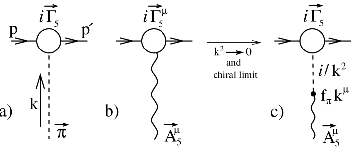
Fig. 6.1: Shown are (a) the proper quark-pseudoscalar vertex coupling to a pion, (b) the proper quark-axial-vector vertex, and (c) the pion decay component of the quark axial-vector vertex which dominates in the soft-pion, chiral limit.

The pion decay constant $f_{\pi}\simeq 93$MeV is defined by the axial-vector transition amplitude for an on-shell pion [$k^{2}=m_{\pi}^{2}$ and $m,n$ are isospin indices]

$$\langle 0|A^{m\sigma}_{5}(0)|\pi^{n}(k)\rangle=i\;f_{\pi}\;k^{\sigma}\;\delta^{mn}\;.$$ (6.19)

From Fig. 6.1(c) and Eq. (6.19) we find then that as $k\to 0$

$$i\vec{\Gamma}^{\sigma}_{5}(p^{\prime},p)\ \smash{\mathop{\longrightarrow}\limits_{k\to 0}}\ \left[i\Gamma^{m}_{5}(p^{\prime},p)\right]\left[{i\over k^{2}}\right]\left[i\langle 0|\vec{A}^{\sigma}_{5}|\pi^{m}(-k)\rangle\right]\smash{\mathop{\longrightarrow}\limits_{k\to 0}}\ -\vec{\Gamma}_{5}(p^{\prime},p)f_{\pi}(k^{\sigma}/k^{2})\;.$$ (6.20)

Acting on both sides of Eq. (6.20) with $k_{\sigma}$, we find the that $k_{\sigma}\vec{\Gamma}^{\sigma}_{5}(p^{\prime},p)\to if_{\pi}\vec{\Gamma}_{5}(p^{\prime},p)$ as $k\to 0$, which when combined with Eq. (6.18) gives the Goldberger-Treiman relation for the quark-pseudoscalar vertex:

$$\vec{\Gamma}_{5}(p,p)=i\vec{\tau}\gamma_{5}\frac{B(p^{2})}{f_{\pi}}=i\vec{\tau}\gamma_{5}\frac{Z^{-1}(p^{2})M(p^{2})}{f_{\pi}}\;.$$ (6.21)

The simplest generalisation of Eq. (6.21) to $k\not=0$ is perhaps

$$\vec{\Gamma}_{5}(p^{\prime},p)=i\;\vec{\tau}\;\gamma_{5}\;{1\over 2}[B(p^{\prime 2})+B(p^{2})]/f_{\pi}\;.$$ (6.22)

However, to properly determine the pseudoscalar vertex away from the soft-pion limit obviously requires solving the pseudoscalar vertex DSE. This is equivalent to the solution of the pion BSE, where the pion Bethe-Salpeter amplitude is defined as

$$\chi^{n}_{\alpha\beta}(p,P)\equiv\int d^{4}z\;e^{i[p-(P/2)]\cdot z}\langle 0|T\psi_{\alpha}(0)\bar{\psi}_{\beta}(z)|\pi^{n}(P)\rangle\;,$$ (6.23)

where $|\pi^{n}(P)\rangle$ denotes a pion state with momentum $P$, $n$ is the isospin label, and $\vec{\chi}$ is related to $\vec{\Gamma}_{5}$ by

$$\vec{\chi}(p,P)=\left[iS\left(p+\frac{P}{2}\right)\right]\left[i\vec{\Gamma}_{5}\left(p+\frac{P}{2},p-\frac{P}{2}\right)\right]\left[iS\left(p-\frac{P}{2}\right)\right]\;.$$ (6.24)

In Eq. (6.23) all colour indices are suppressed. In the amplitude $\chi$ the incoming pion has 4-momentum $P$, the quark has 4-momentum $p+(P/2)$, and the antiquark has 4-momentum $p-(P/2)$. The parity and time-reversal invariance properties of a pseudoscalar imply that we can write

$$\chi(p,P)=\gamma_{5}\chi_{P}(p,P)+\mbox{$\not\!P$}\gamma_{5}\chi_{A}(p,P)+\mbox{$\not\!p$}\gamma_{5}\chi_{A^{\prime}}q(p,P)+[\mbox{$\not\!p$},\mbox{$\not\!P$}]\gamma_{5}\chi_{T}(p,P)\;.$$ (6.25)

Here $\chi_{i}(p,P)$ for $i=P,A,A^{\prime}$, and $T$ are scalar functions of $p^{2},(p\cdot P)$, and $P^{2}$. The subscripts P, A, and T denote the spinor matrix structure of the particular component of $\chi$. The three functions $\chi_{P}$, $\chi_{A}$, and $\chi_{T}$ are even functions of $p\cdot P$, whereas $\chi_{A^{\prime}}$ must be an odd function of $p\cdot P$. A similar expansion can also be made for the proper quark-pseudoscalar vertex $\Gamma_{5}$. In the chiral limit where the pion is massless we obviously have for an on-shell pion $P^{2}=m^{2}_{\pi}=0$.

Using the above it is possible to obtain an expression for $f^{2}_{\pi}$ from the integral equation for pion decay illustrated in Fig. 6.2.

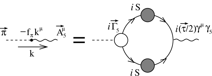
Fig. 6.2: The integral equation for the pion decay constant $(f_{\pi})$.

Our discussion here is a relatively straightforward extension of the arguments presented by Pagels and Stokar (1979,1980) and Cornwall (1980) to the case where $A(p^{2})\neq 1$. From Fig. 6.2 we find that

$$i\langle 0|A^{m\sigma}_{5}(0)|\pi^{n}(k)\rangle = i(ik^{\sigma}f_{\pi}\delta^{mn})=-k^{\sigma}f_{\pi}\delta^{mn}$$ (6.26)

$$= (-1)\int{d^{4}p\over(2\pi)^{4}}\;{\rm tr}\biggl{\{}[iS(p+k)][i\Gamma^{m}_{5}(p+k,p)][iS(p)][i(\tau^{n}/2)\gamma^{\sigma}\gamma_{5}]\biggr{\}}$$

$$= (-1)\int{d^{4}p\over(2\pi)^{4}}\;{\rm tr}\biggl{\{}[\chi^{m}_{5}(k,p)][i(\tau^{n}/2)\gamma^{\sigma}\gamma_{5}]\biggr{\}}\;,$$

where, as usual, the factor [-1] on the RHS arises from the fermion [i.e., quark] loop. In order to avoid double counting we need to take the axial-vector vertex as a perturbative vertex for the same reason as this is done in the photon self-energy diagram in Fig. 2.1. [The argument for $f_{\pi}$ in Williams et al. (1991) is erroneous for this reason, although the error actually has very little effect on the numerical results reported therein.] If, in the limit $k\to 0$ in Eq. (6.26), we equate coefficients of $k^{\sigma}$, using the approximation: $\Gamma_{5}(p^{\prime},p)\approx\Gamma_{5}(p,p)+O(k)\gamma_{5}$; i.e., assuming the Dirac structure of the $O(k)$ correction is purely $\gamma_{5}$, and use the Goldberger-Treiman relation Eq. (6.21) for $\vec{\Gamma}_{5}$, we obtain, in the limit of exact chiral symmetry, [see Appendix C for details]

$$f^{2}_{\pi}=-12i\int{d^{4}p\over(2\pi)^{4}}\;{Z(p^{2})M(p^{2})\over[p^{2}-M^{2}(p^{2})]^{2}}\left[M(p^{2})-{p^{2}\over 2}{dM\over dp^{2}}\right]$$ (6.27)

which as a physical observable must be independent of the choice of renormalisation point, as can be verified numerically for solutions. It should be emphasised that, while this derivation is quite general, the assumed form of $\Gamma_{5}(p^{\prime},p)$ for $p^{\prime}\neq p$ influences the result, which is therefore model dependent. [Another form appears in Eq. (7.57). Both forms reduce to the Pagels and Stokar (1979) result when $Z(p^{2})=A^{-1}(p^{2})=1$ which indicates that the O$(k)$ corrections to $\Gamma_{5}(p^{\prime},p)$ measure deviations from $A(p^{2})\equiv 1$, consistent with the result of Delbourgo and Scadron (1979).] It is straightforward to write down the Euclidean space versions of Eq. (6.16) and Eq. (6.27) by inspection and for completeness these have been given in Appendices B and C respectively.

Numerical Results.       As a specific example of the above arguments for studying DCSB in QCD we describe numerical results from one model DSE for the quark propagator (Hawes et al. , 1993). [Other models and results will be compared and summarised below.] This study uses the Ball-Chiu and Curtis-Pennington vertices together with an Ansatz for the gluon propagator in Landau gauge of the form

$$(g^{2}/4\pi)D^{\nu\sigma}(q)\to\alpha_{s}(Q^{2})D_{0}^{\nu\sigma}(q)$$ (6.28)

with

$$\alpha_{s}(Q^{2})=\alpha_{s}(\tau;Q^{2})\frac{(Q^{2})^{2}}{(Q^{2})^{2}+b^{4}}~{}\;\;\;\;{\rm and}\;\;\;\;\alpha_{s}(\tau;Q^{2})=\frac{d\pi}{\ln\left[\displaystyle\tau+\left(Q^{2}/\Lambda_{\rm QCD}^{2}\right)\right]}~{},$$ (6.29)

where $\ln\tau>0$ [i.e., $\tau>1$] and $b$ are real constants to be determined. This is to be understood in terms of the arguments which lead to Eq. (6.9); i.e., it is understood that the ghost and nonperturbative gluon propagator behaviour have been absorbed into the nonperturbative structure of $\alpha_{s}(Q^{2})$. It is clear that this Ansatz has the asymptotic form of Eq. (2.56) as $Q^{2}\to\infty$. In the infrared, we see that the effective gluon propagator vanishes as $Q^{2}\to 0$; i.e., $D(q)\sim q^{2}/[(q^{2})^{2}+b^{4}]$. [The origins of this form of gluon propagator are discussed in detail in Sec. 5.1.] A closely related study, where the infrared gluon propagator has a Gaussian form and where the Ball-Chiu vertex was used, is described in Hawes and Williams (1991).

We see that the parameter $\tau>1$ plays the dual role of regulating the infrared behaviour of the logarithmic term and of determining the strength of the nonperturbative infrared interaction. Using the quark condensate as an order parameter, we find that there is a critical value of $b=b_{c}$ such that the model does not support dynamical chiral symmetry breaking for $b>b_{c}$.

In Sec. 6.2 we discuss confinement and illustrate a confinement test by applying it to this model. The results suggest that, for all values of $b$, the quark propagator in the model is not confining. Two properties of a particle’s propagator which together are at least sufficient to ensure confinement of the particle are: 1) the absence of a Källen-Lehmann representation and 2) no singularity on the timelike $q^{2}$ axis. This will be discussed in more detail in Sec. 6.2. The gluon propagator implied by Eq. (6.29) satisfies both of these requirements. Although it can be argued that it describes a confined gluon, it may seem that quark confinement is counterintuitive, since it would appear to provide a weak interaction between quarks at small $p^{2}$, corresponding to large distances. Nevertheless, as discussed in Sec. 5.1, quark confinement is not implausible in this model.

We note too that there has been an attempt to employ a gluon propagator similar to Eq. (6.29) in a study of quarkonium spectra by Becker et al. (1991). A Blankenbecler-Sugar reduction of a ladder-like approximation to the BSE is used and it is argued that, in the bound state equation that results, one can approximate the effect of Eq. (6.29) by a Coulomb potential for all $r$.

We can now study the implications of Eq. (6.9) and Eq. (6.29) for the structure of the quark propagator. A similar study has been carried out by Alkofer and Bender (1993). Using Landau gauge [$\xi=0$] since, as discussed earlier, the form of gluon propagator we consider here is most realistic in this gauge, we find that in both the Ball-Chiu and Curtis-Pennington cases there are regions of DCSB and unbroken chiral symmetry characterised by a two-dimensional phase diagram in $(b^{2},\ln\tau)$ space, where $b$ and $\tau$ appear in Eq. (6.29). The phase transition is second order.

For the most part in this study $\Gamma^{\mu}_{\rm CP}(k,p)$ was neglected; i.e., a minimal Ball-Chiu Ansatz was used. This has the virtue of simplifying the integral equations. This term was included for a single value of $\tau$ and a number of values of $b$ and found to generate a small quantitative change in some of the characteristic quantities calculated in the model but not to alter its qualitative features. The integral equations were solved numerically by iteration on a logarithmic grid of $x=p^{2}/\Lambda_{\rm QCD}^{2}$ and $y=k^{2}/\Lambda_{\rm QCD}^{2}$ points. This ensured that the results were independent of the seed-solution and grid choice. The results were independent of the UV cutoff, which was $\Lambda_{\rm UV}^{2}=5\times 10^{8}\;\Lambda_{\rm QCD}^{2}$, and this value was also sufficient to ensure that the leading-log behaviour of the mass function had become evident.

We are interested in determining whether the model gluon propagator specified by Eq. (6.29) can support DCSB - a crucial feature of QCD. The quark condensate, which is gauge-invariant, was studied earlier and is an order parameter for DCSB. In cases for which our iterative solution procedure for the DSE converged quickly, with relative errors of less than $1\times 10^{-6}$, the condensate could be obtained easily. However, for values of $b^{2}$ near a phase transition the convergence could be extremely slow. In those cases, the numerical solution was examined at constant intervals through the run [say, every 50th cycle], and the condensate evaluated in each case. Aitken extrapolation (Wimp, 1981) was then used to find the “infinite-cycles” limit. In several cases the program was subsequently run until the solutions had converged to within $1\times 10^{-6}$ and the extrapolated result always matched the actual result to within a few parts in $10^{-6}$.

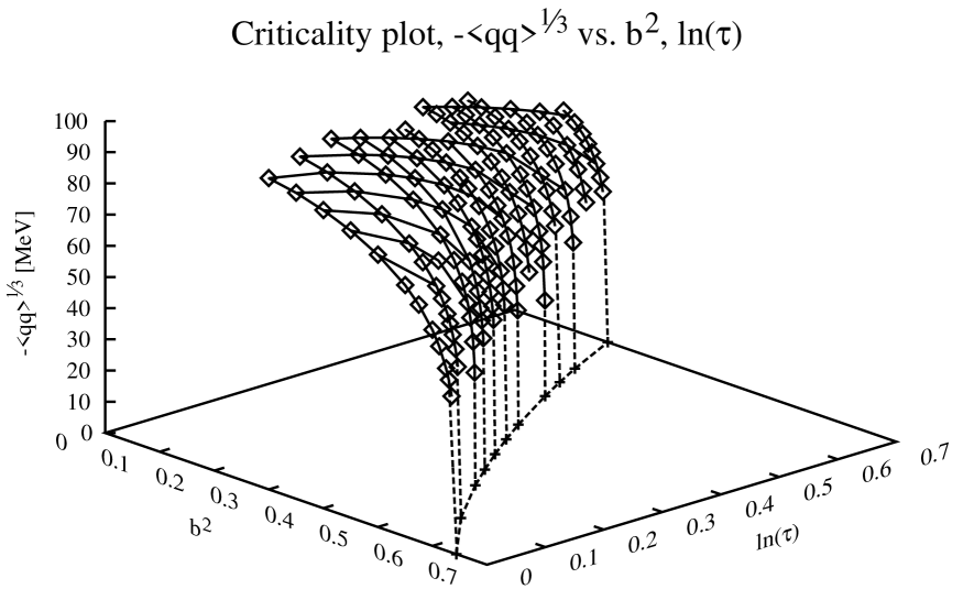
Fig. 6.3: Criticality plot for $(-\langle\bar{q}q\rangle_{\mu})^{\frac{1}{3}}$ as a function of $\ln\tau$ and $b^{2}$. The condensate, $(-\langle\bar{q}q\rangle_{\mu})^{\frac{1}{3}}$, is in units of MeV, scaled to $\mu^{2}=1{\rm GeV}$, and $b^{2}$ is in units $\Lambda_{QCD}^{2}$; the gluon regulator $\tau$ is dimensionless.

We solved Eqs. (6.10) and (6.11) for values of $\ln\tau$ in the domain $[0.0,0.7]$ and $b^{2}$ in $[0.1,1.0]$ using the minimal Ball-Chiu vertex and we plot the condensate obtained from our solutions in Fig. 6.3. This figure shows regions of unbroken and dynamically broken chiral symmetry. Our numerical results suggest that the condensate rises continuously from the transition boundary and hence that the transition is second order. As a consequence we assumed that the order parameter, $\langle\overline{q}q\rangle_{\mu}$, behaves as

$$\langle\overline{q}q\rangle_{\mu}(z)\approx C\left(1-\frac{z}{z_{c}}\right)^{\beta}$$ (6.30)

for $z\rightarrow z_{c}^{-}$ [for z equal to either $\ln\tau$ or $b^{2}$] and extracted the critical points, $z_{c}$, and critical exponents, $\beta$, using ratio-of-logs methods. We list these quantities in Table 6.1 and, in Fig. 6.4, plot the critical curve in the $(b^{2},\ln\tau)$ plane.

Table 6.1: The critical points and exponents extracted for various values of $\ln\tau$; the cumulative result is $\beta_{\rm BC}=0.575$, with $\sigma_{\beta}=0.024$; excluding the point with $\ln\tau=0.0$, $\beta_{\rm BC}=0.572$ with $\sigma_{\beta}=0.020$.

$\ln\tau$	$b^{2}_{\rm C}$ - Critical $b^{2}$ value	$\beta$ - Critical Exponent	$\sigma_{\beta}$ - standard deviation in $\beta$
0.00	0.6439	0.609	0.030
0.10	0.5448	0.579	0.021
0.20	0.4642	0.570	0.021
0.30	0.3932	0.573	0.021
0.40	0.3289	0.567	0.021
0.50	0.2706	0.567	0.021
0.60	0.2180	0.561	0.021
0.70	0.1710	0.579	0.021

Fig. 6.4: Critical curve for the phase transition in the $(\ln\tau,b^{2})$ plane. The asterisk is the result extracted from Roberts and McKellar (1990).

Fig. 6.5: Comparison of the $(-\langle\bar{q}q\rangle_{\mu})^{\frac{1}{3}}$ condensate curves for the minimal Ball-Chiu and Curtis-Pennington Ansätze for the proper vertex. Both curves have $\ln\tau=0.6$. Diamonds, $\diamond$, connected with solid lines are the results from the B-C vertex; plus-signs, $+$, connected with dashed lines are results from the C-P vertex.

We also solved Eqs. (6.10) and (6.11) with the Curtis-Pennington additions, Eqs. (6.12) and (6.13), using $\ln\tau=0.6$. The critical curve [in $b^{2}$] in this case is shown in Fig. 6.5 along with the minimal Ball-Chiu results for the same value of $\ln\tau$. The effect of the Curtis-Pennington addition is to lower the critical value of $b^{2}$ but, as we show below, the critical exponent is unchanged. This curve illustrates the point that the qualitative features of the model are not affected by this modification of the model quark-gluon vertex.

From Table 6.1 we find:

$$\beta_{\rm BC}=0.575\; \;\;{\rm and}\;\; \;\sigma_{\beta}=0.024~{}.$$ (6.31)

We note that the critical exponent obtained with $\ln\tau=0$ is quite different from the others. This is a special case since for this value the propagator does not vanish in the infrared:

$$\frac{g^{2}}{4\pi}D(Q^{2}=0)=d_{\rm M}\pi\,\frac{\Lambda_{\rm QCD}^{2}}{b^{4}}~{}.$$ (6.32)

If we neglect this point in our analysis then we find

$$\beta_{\rm BC}=0.572\; \;\;{\rm and}\;\; \;\sigma_{\beta}=0.020~{}.$$ (6.33)

The results in Eqs. (6.31) and (6.33) are in agreement with those of Roberts and McKellar (1990) where it is argued that $\beta=0.589\pm 0.031$. That study used $b^{2}=0$ and found a critical value of $\ln\tau=1.69$ which complements the results reported here.

We also calculated the critical exponent using our numerical DSE solutions obtained with the Curtis-Pennington addition to the vertex at $\ln\tau=0.6$:

$$\beta_{\rm CP}=0.579 \;\;,\;\; \sigma_{\beta}=0.015~{}.$$ (6.34)

This suggests that the vertex modification does not alter the critical exponent of the transition; a conclusion that is also supported by the observation that the vertex used in Roberts and McKellar (1990) was not of either of the above forms but was, effectively, a simple modified rainbow approximation: $\Gamma_{\mu}(k,p)=A(k^{2})\gamma_{\mu}$.

Other Studies and Results.       There have been numerous studies of DCSB in QCD using the quark DSE and it is unfortunately not possible to give an exhaustive summary of all of them herein. However, all of the studies are well represented by the above exemplary study: each necessarily assumes or argues for one or another form of effective gluon propagator and makes some assumption about the quark-gluon vertex. In addition, many of the earlier studies used the approximation of Eq. (4.7) in order to obtain an approximate differential equation for the quark propagator. Many also used rainbow approximation, Eq. (3.21), in Landau gauge.

There are some interesting early studies by Higashijima (1983, 1984) in Landau gauge and using rainbow approximation with the following Ansatz for the running coupling:

$$\alpha_{s}(Q^{2}<Q_{0}^{2})=\frac{d_{M}\pi}{\ln\left({Q_{0}^{2}/\Lambda_{\rm QCD}^{2}}\right)}\; \;\;{\rm and}\;\; \;\alpha_{s}(Q^{2}>Q_{0}^{2})=\frac{d_{M}\pi}{\ln\left({Q^{2}/\Lambda_{\rm QCD}^{2}}\right)}~{}.$$ (6.35)

Employing Eq. (4.7) in order to obtain a differential equation it was shown (Higashijima, 1984) that for $\ln[Q_{0}/\Lambda_{\rm QCD}]<0.88$, corresponding to $\alpha_{s}(0)\sim 1$, the model admits DCSB. Importantly, it was shown that in order to obtain a differential equation for the mass function whose solution agreed with the one-loop renormalisation group result, Eq. (6.14), one must not neglect derivatives of $\alpha_{s}(Q^{2})$.

Subsequently there were a series of studies by Atkinson and Johnson, (1987, 1988a, 1988b). It was found that in Landau gauge, with

$$\alpha_{s}(Q^{2})=\frac{d_{M}\pi}{\ln\left(\tau+\frac{Q^{2}}{\Lambda_{\rm QCD}^{2}}\right)}~{},$$ (6.36)

with a vertex Ansatz which satisfied the WTI, but which involved kinematic singularities, and using Eq. (4.7), one obtains a differential equation for the mass quark mass function whose solution is such that the model manifests DCSB for $\alpha_{s}(0)>\alpha_{s}^{c}(0)\approx 0.9$ (Atkinson and Johnson, 1988b).

This model was reanalysed by Roberts and McKellar (1990) who solved the integral equations for $A(p^{2})$ and $B(p^{2})$ directly and analysed the reliability of Eq. (4.7). It was found that using Eq. (4.7) the model manifests DCSB for $\alpha_{s}(0)>\alpha_{s}^{c}(0)\approx 0.78$. The difference between this result and that of Atkinson and Johnson (1988b) being due to a more detailed analysis by Roberts and McKellar (1990) of the behaviour of the mass function near the critical coupling. Upon solving the integral directly it was found that the critical coupling increased to $\alpha_{s}^{c}(0)\approx 0.89$: a $12$% rise. The approximation of Eq. (4.7) is thus seen to be qualitatively reliable in this case. This is the best possible application of the approximation, however. It was shown that Eq. (4.7) becomes unreliable as $\alpha_{s}(0)$ is increased making it suspect in any study in which the model gluon propagator is large or singular at $Q^{2}=0$. An important result of this study was that, even in Landau gauge, $A(p^{2})\neq 1$ when the integral equations are solved directly without further approximation. [The same it true in the QED₃ studies described in Sec. 3.]

Equation (4.7) was used by Krein et al. (1988, 1990) in a study of a $1/Q^{4}$ infrared form for the effective gluon propagator, which lead to a confined quark. However, these results were later seen to be completely dependent on the use of the angle approximation to regulate the divergent infrared gluon behaviour. This emphasises the limitations of this approximation discussed by Roberts and McKellar (1990).

The difficulties associated with using a model gluon propagator with a nonintegrable singularity in the infrared in a covariant quark-DSE were are also illustrated in a study by von Smekal et al. (1991). In this study

$$\alpha_{s}(Q^{2})=\frac{d_{M}\pi}{\ln\left(1+\frac{Q^{2}}{\Lambda_{\rm QCD}^{2}}\right)}+d_{M}\pi f(Q^{2})~{},$$ (6.37)

with $f(Q^{2})$ regular as $Q^{2}\rightarrow 0$, and an Ansatz for the quark-gluon vertex was chosen such that it satisfied the Ward identity. This was subsequently approximated in order to simplify the analysis. As in all cases with a $Q^{-4}$ singularity in the model gluon propagator a regularisation procedure was necessary and these authors chose to make the replacement $Q^{2}\rightarrow[Q^{2}+\mu^{2}]$ in the singular part of the running coupling. [A value of $\mu=10^{-4}\Lambda_{\rm QCD}$ was found to reduce the sensitivity of the results to this parameter to less than 1%. This might be compared with the prescription employed by Brown and Pennington (1989), Eq. (5.25).] The coupled, nonlinear integral equations for $A(p^{2})$ and $B(p^{2})$ obtained with $f\equiv 0$ were solved and the model shown to manifest DCSB. However, this version yielded a rather poor phenomenology in the sense that the quark condensates and pion decay constant, $f_{\pi}$, calculated from the solution for the quark propagator, did not agree well with the accepted values. It was found that this could be remedied by using $f(Q^{2})=\gamma^{2}/[Q^{2}+m_{g}^{2}]$ with $\gamma=2.5\Lambda_{\rm QCD}$, $m_{g}=0.2\Lambda_{\rm QCD}$ and $\Lambda_{\rm QCD}=0.5$ GeV. [The value of the effective gluon mass implied by this parameter choice is smaller than the value of $\sim 0.5$ GeV suggested by other studies; for example, those described in Sec. 5.1.]

In many respects this study is qualitatively and quantitatively similar to that of Williams et al. (1991) in which the $Q^{-4}$ singularity was regularised by replacing it with an integrable distribution:

$$\alpha_{s}(Q^{2})=C\,\Lambda_{\rm QCD}^{2}\,Q^{2}\,\delta^{4}(Q)+\frac{d_{M}\pi}{\ln\left(\tau+\frac{Q^{2}}{\Lambda_{\rm QCD}^{2}}\right)}~{}.$$ (6.38)

[The first term alone was studied in rainbow approximation by Munczek and Nemirovsky (1983) and Cahill and Roberts (1985).] Williams et al. (1991) used Landau gauge, a simplified vertex: $\Gamma^{\nu}=(1/2)[A(p^{\prime 2})+A(p^{2})]\gamma^{\nu}$, and solved the coupled, nonlinear integral equations for $A(p^{2})$ and $B(p^{2})$. It was found that once $f_{\pi}$ was fitted by adjusting the infrared coupling strength, $C$, then the quark condensate assumed a value in the typical range, $(-\langle\bar{q}q\rangle)^{1/3}\simeq 225\pm 25$MeV at $\mu=1$GeV. A similar study with the Ball-Chiu vertex and a Gaussian form for the gluon propagator in the infrared reached similar conclusions (Hawes and Williams, 1992).

An effective long-distance quark-quark interaction was derived from dual QCD, which is a long-distance treatment of QCD where the vacuum has the properties of a dual superconductor. The roles of the electric and magnetic fields are interchanged in this picture [for a detailed review see Baker et al. (1991)]. This effective quark interaction was then used as input into studies of DCSB [see Bakeret al. (1988) and Krein and Williams (1991)] with some success. It is unfortunate, that a sign error was recently detected in the original derivation by S. Kamizawa [Baker et al. (1988, erratum 1991)], which leaves open the question of whether or not DCSB occurs naturally in dual QCD. Studies of DCSB have also been generalised to a chromodielectric model of QCD where a mean field treatment of the colour-dielectric constant and DCSB arguments leads to a chiral, nontopological soliton model (Krein et al., 1988, 1991).

A model gluon propagator that is not singular in the infrared has also been studied (Haeri and Haeri, 1991; Papavassiliou and Cornwall, 1991). Haeri and Haeri (1991) use

$$\frac{\alpha_{s}(Q^{2})}{Q^{2}}\sim\frac{1}{Q^{2}+m^{2}}\frac{1}{\ln\left(\frac{Q^{2}+4m^{2}}{\Lambda_{\rm QCD}^{2}}\right)}~{},$$ (6.39)

based on the analysis by Cornwall (1982), where $m$ is an effective gluon mass, and a vertex Ansatz constructed so as to eliminate overlapping divergences in the quark DSE. As one would expect in such a model, there is a critical value of the ratio $m/\Lambda_{\rm QCD}=R_{m}^{c}$ such that only for $m/\Lambda_{\rm QCD}<R_{m}^{c}$ does the model manifest DCSB. In this particular model, however, such a result is phenomenologically inconsistent because it means that DCSB requires an effective gluon mass which is significantly less than the value of $\sim 0.5$ GeV suggested by other studies [see Sec. 5.1]. A similar internal inconsistency was found by Papavassiliou and Cornwall (1991) in their study of approximate coupled DSEs for the 3-gluon and quark-gluon vertices and subsequent analysis of the DSE for the quark propagator. The conclusion in both of these studies is that confinement is not incorporated in the model specified by Eq. (6.39) whose infrared behaviour therefore requires modification if a reasonable phenomenological model of DCSB is to be obtained.

There have also been studies of the non-covariant, Coulomb-gauge, quark DSE (Finger and Mandula, 1982; Govaerts et al., 1983, 1984; Alkofer and Amundsen 1988; Langfeld et al., 1989). As in the covariant studies, it is found that one has DCSB if the coupling at zero momentum transfer exceeds a critical value. We remark that Alkofer and Amundsen (1988) used a model interaction with $\alpha(|\vec{Q}|^{2})\sim|\vec{Q}|^{-2}$ which was regularised using a cutoff mass: $|\vec{Q}|^{2}\rightarrow[|\vec{Q}|^{2}+\mu^{2}]$. In all cases a not unreasonable phenomenological description of DCSB was obtained.

Summary.       The body of work exemplified and summarised in this section clearly demonstrates that a very good phenomenological description and understanding of DCSB in QCD can be obtained using the DSE for the quark self energy. Given a gluon propagator whose behaviour at large spacelike-$q^{2}$; i.e., in the ultraviolet, is given by the renormalisation group in QCD and whose behaviour at small spacelike-$q^{2}$; i.e., in the infrared, yields an effective coupling strength that is $>1$, then one will have $\langle\overline{q}q\rangle\neq 0$. With just one or two parameters to describe the transition from the known behaviour of the gluon propagator in the ultraviolet to the unknown behaviour in the infrared [see Sec. 5.1], one can obtain a good phenomenology of DCSB; i.e., one can obtain values for quantities such as the quark condensates and the pion decay constant that agree with those extracted from experiment. This will be discussed in more detail in Sec. 7.

6.2 Quark Confinement

General Observations and Remarks.       It is now generally accepted that QCD is the appropriate theory for describing the strong interaction. The lack of observation of free quarks and gluons [and ghosts] leads then to the assumption of colour confinement; i.e., that only quantities which transform as colour-singlets can be physical observables. Theoretical studies also lend credence to this expectation, where, for example, lattice gauge theory studies are consistent with a string tension or linearly rising potential between coloured objects. The fact that QCD is a gauge theory also implies that physical observables must be gauge invariant. The BRS invariance properties of QCD can be used to show that the $S$-matrix is gauge invariant, [see Itzykson and Zuber (1980, pp. 604–605)]. At the observational level, the confinement of colour is the statement that the cross-section for the production of any combination of asymptotic coloured states from a colour-singlet initial state must be zero. A more extensive treatment of some of the following discussion can be found in Roberts et al. (1992).

The failure of the cluster decomposition property [CDP] of vacuum expectation values of the coloured fields in QCD [the QCD Wightman functions] is certainly sufficient to ensure confinement [Marciano and Pagels (1978), Greenberg (1978), Strocchi (1976,1978); also see Streater and Wightman (1980) for a discussion of the CDP]. The CDP can be associated with charge screening and so, in simple terms, the failure of the CDP means that, irrespective of how large one makes the spacelike separation between two coloured objects, the interaction between them never becomes negligible. This is the common intuitive basis for understanding confinement that underlies the idea of a string tension in QCD and provides a basis for the linear and harmonic-oscillator potential models. In QED the locality property of the field theory is sufficient to ensure that the CDP is satisfied (Strocchi, 1976, 1978), however, the proof used in QED to demonstrate this property fails in QCD. Crucial to the failure of this proof is the fact that an indefinite metric is unavoidable in local gauge theories and further that QCD is asymptotically free. Of course, the failure to prove the CDP is not equivalent to proving its failure. It is interesting that in QED₂, which has a linear potential, the failure of the CDP can be explicitly demonstrated (Strocchi, 1976).

The $n$-point Green’s functions of a quantum field theory are the time-ordered vacuum expectation values $G^{(n)}(x_{1},\dots,x_{n})\equiv\langle{\rm vac}|T(\phi(x_{1})\dots\phi(x_{n}))|{\rm vac}\rangle$, where here the field operators $\phi$ generically represent gluon, quark, and ghost field operators in QCD. The Wightman functions are simply Green’s functions without time-ordering; i.e., $W^{(n)}\equiv\langle{\rm vac}|\phi(x_{1})\dots\phi(x_{n})|{\rm vac}\rangle$. The CDP is that as $\lambda\to+\infty$

$$W^{(n)}(x_{1},\dots,x_{j},x_{j+1}+\lambda a,\dots,x_{n}+\lambda a) \longrightarrow W^{(j)}(x_{1},\dots,x_{j})\,W^{(n-j)}(x_{j+1},\dots,x_{n})\;,$$ (6.40)

where $a$ is an arbitrary spacelike vector. The actual CDP requirement is more than this. In theories with a mass gap [no zero mass states] the difference between the LHS and RHS of Eq. (6.40) must decrease exponentially, whereas for theories without a mass gap [e.g., QED₄] the decrease must be at least as fast as $1/\lambda^{2}$, (Strocchi, 1976, 1978). No explicit proof that the CDP fails for coloured Wightman functions in QCD is currently known, although the fact that the usual QED proof of this property does not apply in QCD is certainly suggestive. Clearly, if all the $W$ in Eq. (6.40) are colour singlets then the CDP is expected to hold. The failure of the CDP property does not necessarily entail the absence of free coloured states in the spectrum of the theory, e.g., in Greenberg (1978) an effort was made to construct an explicit confining, nonrelativistic, harmonic-oscillator model in which the CDP fails.

A different perspective is discussed in Nishijima (1986) where the non-Abelian nature of QCD and the necessity of an indefinite metric give rise to confinement as a result of the complete cancellation of colour states from the S-Matrix, in a manner analogous to that in which the longitudinal and scalar photons decouple in QED. The mechanism is associated with the extended gauge transformations manifest in the BRS invariance of QCD. In simple terms, this picture of confinement corresponds to the idea that after averaging over gauge field configurations only the colour singlet pieces of operator expectation values remain. This can also be related to the breakdown of the CDP for coloured states.

Another sufficient condition for confinement is if QCD has only colour-singlet free [i.e., on-shell] states. Hence confinement might be equivalent to the statement that the propagator of a coloured state should have no singularities on the real, positive $p^{2}$-axis, [see, e.g., Cornwall (1980), Krein et al. (1988,1990), Gogokhia and Magradze (1989)]. Note that any singularities on the negative [i.e., spacelike] $p^{2}$-axis would imply tachyonic behaviour and hence are not allowed by causality considerations. To discuss this possible form of confinement we will concentrate on the quark propagator, the most general form of which [in an arbitrary covariant gauge] is given in Eq. (2.68). This statement means that the quarks have no mass-pole $M^{2}(\mbox{$p^{2}$})\not=\mbox{$p^{2}$}~{}\mbox{for any }\mbox{$p^{2}$}\geq 0$, and so cannot go on mass shell. It might be argued that if the propagator has a timelike singularity, then it should have a mass-shell and hence there appears to be nothing to prevent us from defining the corresponding free state. [It is always possible to imagine $M(p^{2})$ having some very unusual behaviour at the singular point of the propagator, which would complicate this argument.] This suggests that confinement might be synonymous with the requirement that coloured particles and bound states have no poles in their propagators. [As a counter-example one might consider QCD₂ in which, at leading order in a $1/N_{c}$ expansion, confinement is ensured in a conspiratorial fashion: the quark propagator has a mass pole but the vertex in the BSE has zeros at the momenta which correspond to one of the quarks going on-shell and hence there is no scattering out of the bound state (Einhorn, 1976).]

We remark here that we are discussing the gauge-fixed quark propagator which is a well defined and nontrivial element of field theory and is an important input to any covariant calculation of scattering or bound state amplitudes. This propagator is gauge-dependent but does contain gauge invariant information; e.g., the quark condensate. Of course, a nonzero value of $\langle\overline{q}q\rangle$ does not imply confinement. Our remarks here are meant simply to emphasise that there is gauge invariant content in propagators. A separation between the scales for confinement and dynamical chiral symmetry breaking is, in general, to be expected and DCSB is certainly possible without confinement.

It might be argued that the analytic structure of the gauge-fixed quark propagator would be a genuine signal of confinement in QCD only if the presence or absence of a pole [or branch cut] was also a gauge invariant property. In this connection the Nielsen Identities (Nielsen, 1975) of QCD are important. These identities, derived using the BRS invariance of QCD, ensure that, for example, the quark mass value obtained from the QCD effective action is gauge invariant. This gauge invariance is a result of the cancellation between the gauge dependence of the effective action and that of the vacuum configuration. Hence, one can infer from this that the absence of a mass pole [or branch point] is also a gauge invariant property of the theory. Practically, however, there is a problem with the effective action approach: a non-perturbative calculation of the QCD effective action is prohibitively difficult.

Given the possible implications for confinement it is of interest to examine the consequences of assuming that the quark propagator has no singularities on the real $p^{2}$-axis. We see that the quark propagator will have a mass pole when $M^{2}(\mbox{$p^{2}$})=\mbox{$p^{2}$}$ provided that $Z(\mbox{$p^{2}$})$ is not zero in the neighborhood of this value of $p^{2}$. Alternatively, we might have that $Z$ goes to zero in just the right way to cancel a singularity of the type $1/[\mbox{$p^{2}$}-M^{2}(\mbox{$p^{2}$})]$ or that $Z$ should be zero over a finite region containing just this value of $p^{2}$. In the absence of compensating zeros in $Z$ then we would be left with the requirement that $M^{2}(\mbox{$p^{2}$})\neq\mbox{$p^{2}$}$ for any real $p^{2}$. On perturbative grounds we expect the same behaviour in the asymptotic timelike and spacelike regimes. The only way that $M(\mbox{$p^{2}$})$ can be finite in the deep timelike and spacelike regions of $p^{2}$ and yet never have a pole at $M^{2}(\mbox{$p^{2}$})=\mbox{$p^{2}$}$, for any real $p^{2}$, is if $M(\mbox{$p^{2}$})$ is discontinuous across the $p^{2}$ line or if $Z(\mbox{$p^{2}$})$ has a compensating zero. The possible implications of complex poles in the propagators are discussed in Sec. 5.

As a further observation regarding the absence of mass poles for coloured states we remark that this would imply, for example, that the quark and gluon propagators have no singularities on the real axis. Consider then Eq. (6.9) and assume that $\Gamma^{\nu}$ has no poles [e.g., $\Gamma^{\nu}\to\gamma^{\nu}$ as for the rainbow or ladder approximation] and that the integral exists. We see that the RHS of this equation will be pure imaginary if $\Sigma$ is initially pure real, and hence in general this DSE will give rise to a complex self-energy. This represents an additional complication if this picture of confinement is pursued. We note, however, that if we assume that it is reasonable to begin with the Euclidean transcription of Eq. (6.9) then the quark self-energy will be real. Apparently then, in this confinement scenario the naive Wick rotation is not valid, which should not be surprising.

There is one further point that it is interesting to consider here. Marciano and Pagels (1978) have discussed the possibility of confinement occurring through the power counting of divergences, which were presumed to arise in a full solution for the various propagators and proper vertices of QCD. If confinement results from the non-Abelian nature of QCD then these divergences would also be expected to have non-Abelian origins. At the simplest level one could imagine, for example, associating with each coloured leg of an $n$-point Green’s function a factor $\sqrt{\epsilon}$, while for colour-singlet bound-state legs the factor would be unity. Similarly, for proper [i.e., one-particle irreducible] vertices coloured legs would carry a factor $1/\sqrt{\epsilon}$ and colour-singlet legs again would have the factor 1. It follows that $S$ and $D$ $\sim\epsilon$, $\Gamma^{\nu}\sim 1/\epsilon^{(3/2)}$ for the quark-gluon vertex, $\overrightarrow{\Gamma_{5}}\sim 1/\epsilon$ for the quark-pion vertex, etc. It is straightforward to see that any process with only colour-singlet external legs is of ${\cal O}(1)$, while any process with $m$ coloured external legs will be of ${\cal O}(\epsilon^{(m/2)})$ and so will be completely suppressed as $\epsilon\to 0$. In any perturbative QCD calculations the selection of only those soft final state interactions which give rise to colour singlet asymptotic states is thus ensured. [Many other power counting schemes are possible and may incorporate ghost fields etc. but this illustration exemplifies the general idea behind them.] This is an example of the failure of the CDP for non-colour-singlet asymptotic states, whereas it would not fail for allowed colour-singlet processes. It can simultaneously be considered as an example of the absence of coloured states since free quarks cannot propagate as $\epsilon\to 0$. We do not argue that this is a realistic picture of confinement, rather we take it as a lesson that confinement might arise from subtly cancelling and possibly momentum-dependent divergences in the Green’s functions and proper vertices of QCD.

To summarise: The failure of the cluster decomposition property is sufficient to ensure confinement and forms the basis for many intuitive arguments and simple nonrelativistic models of confinement. One can think of the CDP as a measure of charge screening: having the CDP in a theory means that the interaction is screened and falls off with separation. Failure of Eq. (6.40), when $W^{(j)}$ and $W^{(n-j)}$ are not colour singlets, is consistent with the notion that colour-charge is anti-screened. There is as yet, however, no proof that the CDP fails in QCD. In simple models the failure of the CDP appears linked to this infrared behaviour. The absence of a pole at timelike momenta in a particle’s propagator is also sufficient to ensure confinement [although not necessary, as the QCD₂ example shows (Einhorn, 1976)]. It is certainly conceivable that the failure of the CDP and the absence of a pole in the propagator of confined particles are related and that one is not possible without the other. This interesting speculation receives some support in the simple model described in the next section. Explicit demonstrations of confinement in more realistic models are still wanting, however.

Examples of Confining Models.       Let us consider two simple models of the quark DSE which indeed lead to a confined quark and gluon. More details of this work can be found in Burden et al. (1992b). We work in Euclidean space and use the notation of Burden et al. (1992b), where we write for the quark self-energy $\Sigma(k)=S^{-1}(k)-S_{0}^{-1}(k)$ with the renormalised quark propagator

$$S(k) = \frac{1}{i\gamma\cdot kA(k^{2})+B(k^{2})}=\frac{Z(k^{2})}{i\gamma\cdot k+M(k^{2})}$$ (6.41)

$$= -i\gamma\cdot k\sigma_{V}(k^{2})+\sigma_{S}(k^{2})$$ (6.42)

and the perturbative quark propagator $S_{0}(k)=1/(i\gamma\cdot p+m)$.

The first model of interest is obtained with the choice (Munczek and Nemirovsky, 1983)

$$g^{2}D_{\mu\nu}(k)=D^{0}_{\mu\nu}(k)\;8\pi^{4}D\,k^{2}\,\delta^{4}(k)$$ (6.43)

where $D_{\mu\nu}^{0}(k)=(\delta_{\mu\nu}-k_{\mu}k_{\nu}/k^{2})/k^{2}$ and

$$\Gamma_{\mu}(k,p)=\gamma_{\mu}~{}.$$ (6.44)

This is an infrared dominant model which underestimates the strength of the interaction in QCD at large-$k^{2}$. In a study whose focus is confinement this is not unreasonable since confinement is expected to be a predominantly infrared effect. The quark-quark interaction resulting from Eq. (6.43) is a constant in configuration-space and so the usual proof of the CDP will fail. Using Eq. (6.43) and (6.44), we find that Eq. (6.7) reduces to the following pair of coupled, algebraic equations for $Z(p^{2})$ and $M(p^{2})$ :

$$Z=\frac{M}{2M-m}~{}, 0=2M^{4}-3mM^{3}+M^{2}(2p^{2}-D+m^{2})-3mp^{2}M+p^{2}m^{2}~{}.$$ (6.45)

For $m=0$ there is a dynamical chiral symmetry breaking solution of these equations ($s=p^{2}$)

$$M(s) = \left\{\begin{array}[]{ll}\sqrt{\mbox{$\frac{1}{2}$}D-s}~{},&s<\mbox{$\frac{1}{2}$}D\\ 0~{},&s>\mbox{$\frac{1}{2}$}D\end{array}\right.$$ (6.48)

$$Z(s) = \left\{\begin{array}[]{ll}\frac{1}{2}~{},&s<\mbox{$\frac{1}{2}$}D\\ \displaystyle\frac{s}{2D}\left(\sqrt{1+\frac{4D}{s}}-1\right)~{},&s>\mbox{$\frac{1}{2}$}D\end{array}\right.$$ (6.51)

The CJT effective action [Cornwall et al. (1974)] evaluated at its extremals is (Stam, 1985; Sec. 7.2) when evaluated in Euclidean space:

$$V[S]=\int\frac{d^{4}q}{(2\pi)^{4}}\,\left\{\mbox{trln}[S_{0}^{-1}(q)S(q)]+\mbox{\small$\frac{1}{2}$}\mbox{tr}[\Sigma(k)S(k)]\right\}$$ (6.52)

and is the same as the auxiliary field effective action in this case (McKay and Munczek, 1989). To determine whether chiral symmetry is dynamically broken for m=0 one must evaluate the difference

$$\beta = V[Z=(s/2D)\left(\sqrt{1+4D/s}-1\right),~{}M=0]-V[Z=\mbox{Eq.~{}(\ref{Zz})},~{}M=\mbox{Eq.~{}(\ref{Mz})}]$$ (6.53)

$$= N_{c}N_{f}\frac{D^{2}}{32\pi^{2}}\left(4\ln 2-\frac{11}{4}\right)>0$$

which reveals that the ground state with a nonzero fermion mass function is dynamically favoured and hence chiral symmetry is dynamically broken in this approximation. The dynamical chiral symmetry breaking solution is also a confining solution since $S(p)$ constructed from these functions has no pole on the real $s$ axis. This feature survives for $m>0$ with $M$ and $Z$ smooth on the real $s$ axis: in the spacelike UV limit

$$\begin{array}[]{lcr}\displaystyle M(s)=m\left(1+\frac{D}{s}\right)&\;\;\mbox{and}&\displaystyle Z(s)=1-\frac{D}{s}~{};\end{array}$$ (6.54)

while in the timelike UV limit

$$\begin{array}[]{lcr}\displaystyle M(s)=M_{0}(s)+m\frac{3D}{8}\frac{1}{M_{0}^{2}(s)}&\;\;\mbox{and}&\;\displaystyle Z(s)=Z_{0}(s)+m\frac{1}{4}\frac{1}{M_{0}(s)}~{},\end{array}$$ (6.55)

where $M_{0}$ and $Z_{0}$ are the $m=0$ solutions of Eqs. (6.48) and (6.51). In this case the integrable $\delta^{4}(k)$ singularity in the model gluon propagator of Eq. (6.43) lies behind the absence of singularities in the quark propagator and has been used as the starting point for confining, phenomenological models of nonperturbative QCD [see, e.g., Praschifka et al. (1989) and Frank et al. (1991)].

The second model has the same form for the gluon propagator as Eq. (6.43), but uses the Curtis-Pennington vertex of Eq. (6.5). This represents a test of whether the absence of a pole in the quark propagator is sensitive to the details of the quark-gluon vertex. Substituting Eqs. (6.5) and (6.43) into (6.7) then, instead of Eqs. (6.45), we obtain the following pair of coupled, nonlinear, differential equations:

$$\mu^{\prime}(x) = \frac{2\mu}{x}+2\frac{x+\mu^{2}(x)}{x\zeta(x)}(\zeta(x)\mbox{$\overline{m}$}-\mu(x))~{},$$ (6.56)

$$\zeta^{\prime}(x) = \frac{\mu(x)\mu^{\prime}(x)-1}{x+\mu^{2}(x)}\,\zeta(x)+2(1-\zeta(x))$$ (6.57)

where $x=s/(2D)$, $\mbox{$\overline{m}$}=m/\sqrt{2D}$, $M(s)=\sqrt{2D}\mu(x)$ and $Z(s)=\zeta(x)$. [Note that the transverse addition Eq. (6.3) does not survive when Eq. (6.43) is used and so the Ball-Chiu vertex of Eq. (6.2) gives the same results.] The boundary conditions for these equations are, of course:

$$\begin{array}[]{lcr}\mu(x\rightarrow+\infty)=\mbox{$\overline{m}$}&\;\;\mbox{and}&\zeta(x\rightarrow+\infty)=1\end{array}$$ (6.58)

consistent with Eq. (6.54). The pragmatic benefit of Eq. (6.43) is again obvious: we are confronted with differential equations instead of integral equations [e.g., Roberts and McKellar (1990), Haeri and Haeri (1991), Williams et al. (1991), Hawes and Williams (1991), Hädicke (1991)]. Hence we can obtain solutions for both spacelike and timelike momenta, which enables a study of the singularity structure of the quark propagator. [The infrared dominant $k^{-4}$ model also has this feature in axial gauge as discussed in Ball and Zachariasen (1981).] These differential equations take a particularly simple form when expressed in terms of $\mbox{$\overline{\sigma}_{V}$}(x)=\zeta(x)/(x+\mu^{2}(x))$ and $\mbox{$\overline{\sigma}_{S}$}(x)=\mbox{$\overline{\sigma}_{V}$}(x)\mu(x)$  ($x=k^{2}/(2D)$, $\sigma_{V}(k^{2})=\mbox{$\overline{\sigma}_{V}$}(x)/(2D)$, $\sigma_{S}(k^{2})=\mbox{$\overline{\sigma}_{S}$}(x)/\sqrt{2D}$):

$$\mbox{$\overline{\sigma}_{S}$}^{\prime}(x)=2[\mbox{$\overline{m}$}\,\mbox{$\overline{\sigma}_{V}$}(x)-\mbox{$\overline{\sigma}_{S}$}(x)]~{}, \mbox{$\overline{\sigma}_{V}$}^{\prime}(x)=-\frac{2}{x}[\mbox{$\overline{\sigma}_{V}$}(x)\,(x+1)+\mbox{$\overline{m}$}\,\mbox{$\overline{\sigma}_{S}$}(x)-1]~{}.$$ (6.59)

We begin by considering the $\mbox{$\overline{m}$}=0$ case [in which case Eqs. (6.59) decouple]. Obviously there is the trivial $\mu\equiv 0$ solution that corresponds to a Wigner-Weyl realisation of chiral symmetry. In this case

$$\zeta(x)=1-\frac{1}{2x}+C\frac{\mbox{e}^{-2x}}{x}$$ (6.60)

with $C$ an arbitrary constant. The choice $C=1/2$ yields a propagator with no singularity on the real $x$ axis and is required if this solution of the differential equation is to be consistent with the integral equation, so that there is no singularity within the Euclidean integration domain [in agreement with footnote 3 in Munczek (1986)]. The solution can therefore be written as:

$$\mbox{$\overline{\sigma}_{V}$}(x)=\frac{2x-1+\mbox{e}^{-2x}}{2x^{2}}~{}, \mbox{$\overline{\sigma}_{S}$}(x)=0~{}.$$ (6.61)

There is also a nontrivial solution. In searching for this solution one finds that for $\mbox{$\overline{m}$}=0$ Eqs. (6.56) and (6.57) are scale invariant; i.e., given $\mu$ and $\zeta$ as solutions then

$$\begin{array}[]{lcr}\mu_{\lambda}(x)=\lambda\mu(x)&\;\;\mbox{and}&\;\displaystyle\zeta_{\lambda}(x)=\frac{x+\lambda^{2}\mu^{2}(x)}{x+\mu^{2}(x)}\,\zeta(x)\end{array}$$ (6.62)

are also solutions. It is therefore sufficient to find the solution for which $\mu(0)=1$. These scale transformations correspond to:

$$\begin{array}[]{lcr}\overline{\sigma}_{S}^{\lambda}(x)=\lambda\mbox{$\overline{\sigma}_{S}$}(x)&\;\;\mbox{and}&\;\displaystyle\overline{\sigma}_{V}^{\lambda}(x)=\sigma_{V}(x)\end{array}$$ (6.63)

and the scale invariance of Eqs. (6.56) and (6.57) is a result of the decoupling of Eqs (6.59). It is, of course, easiest to find the solution from Eqs (6.59) which yield $\overline{\sigma}_{V}$ of Eq. (6.61) and

$$\mbox{$\overline{\sigma}_{S}$}(x)=\mbox{e}^{-2x}$$ (6.64)

which correspond to:

$$\mu(x)=\frac{2x^{2}}{1+(2x-1)\,\mbox{e}^{2x}}~{}, \zeta(x)=\frac{4x^{3}+\left[1+(2x-1)\,\mbox{e}^{2x}\right]^{2}}{2x\,\mbox{e}^{2x}\,[1+(2x-1)\,\mbox{e}^{2x}]}$$ (6.65)

To determine whether chiral symmetry is dynamically broken in this model one must evaluate the difference

$$V[\mbox{$\overline{\sigma}_{V}$}=\mbox{Eq.~{}(\ref{svmzro})},\mbox{$\overline{\sigma}_{S}$}=0]-V[\mbox{$\overline{\sigma}_{V}$}=\mbox{Eq.~{}(\ref{svmzro})},\mbox{$\overline{\sigma}_{S}$}=\mbox{Eq.~{}(\ref{ssmzro})}]$$ (6.66)

$$\;\;\;\;\;\;\;\;\;\;\;\;\;\;\;\;\;\;\;\;\;\;\;\;\;\;\;\;\;\;\;\;=-2N_{c}N_{f}\int\mbox{$\displaystyle\frac{d^{4}q}{(2\pi)^{4}}$}\,\ln\left(1+\frac{\mu^{2}(q^{2})}{q^{2}}\right)<0$$

and hence the chirally symmetric solution is dynamically favoured in this case, as pointed out by Munczek (1986). The underlying reason for this is the decoupling of the equations for $\overline{\sigma}_{V}$ and $\overline{\sigma}_{S}$. It is reasonable to expect that with a model gluon propagator that incorporates asymptotic freedom [i.e., one which behaves as $\sim[q^{2}\ln(q^{2})]^{-1}$ in the deep spacelike region] these equations will not decouple and hence chiral symmetry will be dynamically broken.

Comparing these two confining models with $\mbox{$\overline{m}$}=0$ we see that the choice of vertex has a quite dramatic qualitative and quantitative effect on the nature of the solution and the realisation of chiral symmetry. Qualitatively, the dressed vertex has ensured that the quark propagator is an entire function, whereas in the bare vertex case it had a branch point at $x=1/4$, and it has also eliminated dynamical chiral symmetry breaking from the model. Quantitatively, there is a dramatic enhancement of the propagator at large $(-x)$; i.e., the deep timelike region. This is easily seen since, using Eq. (6.44), one finds that in the bare vertex case $\mbox{$\overline{\sigma}_{V}$}(x=k^{2}/(2D))\rightarrow 2$ and $\mbox{$\overline{\sigma}_{S}$}(x)\rightarrow 2\sqrt{-x}$ as $x\rightarrow-\infty$ which are to be compared with Eqs. (6.61) and (6.64).

In the second model with $\mbox{$\overline{m}$}\neq 0$ there is no trivial [$\mu\equiv 0$] solution and solving Eqs. (6.56) and (6.57) [or, equivalently, Eqs. (6.59)] is a little more difficult. These equations can be combined to yield:

$$\frac{d^{2}}{dx^{2}}\mbox{$\overline{\sigma}_{S}$}(x)+4\left(1+\frac{1}{2x}\right)\frac{d}{dx}\mbox{$\overline{\sigma}_{S}$}(x)+4\left(1+\frac{1+\mbox{$\overline{m}$}^{2}}{x}\right)\mbox{$\overline{\sigma}_{S}$}(x) = \frac{4\mbox{$\overline{m}$}}{x}$$ (6.67)

from which one obtains ($x=y^{2}$):

$$\mbox{$\overline{\sigma}_{S}$}(y)=\frac{c_{1}}{2\mbox{$\overline{m}$}y}\,\exp(-2y^{2})\,J_{1}(4\mbox{$\overline{m}$}y)+\frac{\mbox{$\overline{m}$}^{2}}{y}\int_{0}^{\infty}d\xi\,\xi K_{1}(\mbox{$\overline{m}$}\xi)J_{1}(y\xi)\mbox{e}^{-\frac{\xi^{2}}{8}}$$ (6.68)

with $c_{1}$ an undetermined constant and $J_{1}$ and $K_{1}$ Bessel and modified Bessel functions of order one, respectively. [In the limit $\mbox{$\overline{m}$}\rightarrow 0$ Eq. (6.68) reduces to Eq. (6.64); the dynamical chiral symmetry breaking solution. In the following we set $c_{1}=0$ and concentrate on the behaviour of that part of the solution associated with explicit chiral symmetry breaking.] The form of $\overline{\sigma}_{V}$ follows from Eq. (6.59) ($y^{2}=x$):

$$\mbox{$\overline{\sigma}_{V}$}(y)=\frac{1}{\mbox{$\overline{m}$}}\left(\mbox{$\overline{\sigma}_{S}$}(y)+\frac{1}{4y}\frac{d}{dy}\mbox{$\overline{\sigma}_{S}$}(y)\right)~{}.$$ (6.69)

It is clear that $\mbox{$\overline{\sigma}_{V}$}(y)$ and $\mbox{$\overline{\sigma}_{S}$}(y)$ are even under $y\rightarrow\,-y$ and, hence, are functions of $x=y^{2}$. Further, after a little thought it becomes clear that $\mbox{$\overline{\sigma}_{S}$}(x)$ and $\mbox{$\overline{\sigma}_{V}$}(x)$ are entire functions in the complex $x$ plane. A combination of numerical and analytic methods establishes that both $\overline{\sigma}_{S}$ and $\overline{\sigma}_{V}$ are positive definite on the real $x$-axis. It is of interest to determine the asymptotic behaviour of these functions at large spacelike and timelike $x=k^{2}/(2D)$. In the deep spacelike region [$x\sim+\infty$] one finds easily that $\mbox{$\overline{\sigma}_{S}$}(x)=\mbox{$\overline{m}$}/x$ and $\mbox{$\overline{\sigma}_{V}$}(x)=1/x$. In the deep timelike region ($x\sim-\infty$) the analysis is a little more complicated. Using Laplace’s method one finds that at large $E=\sqrt{-x}$:

$$\mbox{$\overline{\sigma}_{S}$}(E)=\sqrt{\frac{\pi\mbox{$\overline{m}$}^{3}}{2E^{3}}}\exp\left(2[E-\mbox{$\overline{m}$}]^{2}\right)\left[1+\mbox{erf}\left(\sqrt{2}[E-\mbox{$\overline{m}$}]\right)\right]$$ (6.70)

which yields the following asymptotic timelike behaviour:

$$\mbox{$\overline{\sigma}_{S}$}(E) = \sqrt{\frac{2\pi\mbox{$\overline{m}$}^{3}}{E^{3}}}\exp\left(2[E-\mbox{$\overline{m}$}]^{2}\right)~{},$$ (6.71)

$$\mbox{$\overline{\sigma}_{V}$}(E) = \sqrt{\frac{8\pi\mbox{$\overline{m}$}}{E^{3}}}\exp\left(2[E-\mbox{$\overline{m}$}]^{2}\right)\left(1-\frac{\mbox{$\overline{m}$}}{2E}-\frac{3}{16E^{2}}\right)~{}.$$ (6.72)

This again is a dramatic enhancement compared with the bare vertex solutions: $\mbox{$\overline{\sigma}_{V}$}\simeq 2(1-\mbox{$\overline{m}$}/\sqrt{\frac{1}{4}-x})$ and $\mbox{$\overline{\sigma}_{S}$}\simeq 2(\sqrt{\frac{1}{4}-x}-\mbox{$\overline{m}$})$.

Hidden in this discussion of $\overline{\sigma}_{S}$ and $\overline{\sigma}_{V}$ is the behaviour of the functions $\mu$ and $\zeta$ [which are related to the mass function, $M$, and wave function renormalisation, $Z$: see after Eq. (6.57)] that can be expressed [$K(x)=1+\mbox{$\overline{\sigma}_{S}$}^{\prime}(x)/(2\mbox{$\overline{\sigma}_{S}$}(x)$]:

$$\mu(x)=\frac{\mbox{$\overline{\sigma}_{S}$}(x)}{\mbox{$\overline{\sigma}_{V}$}(x)}\equiv\frac{\mbox{$\overline{m}$}}{K(x)}\; \;\;{\rm and}\;\; \zeta(x)=\frac{1}{\mbox{$\overline{m}$}}\left[x+\mu^{2}(x)\right]\mbox{$\overline{\sigma}_{S}$}(x)K(x)~{}.$$ (6.73)

The propagator is very often discussed and modelled in terms of these functions [equivalent to $M$ and $Z$]. Our analysis leads us to the conclusion that $K(x)>0$ for all finite, real $x$ and hence so is $\mu$; i.e., the mass function has no zeros or singularities for real $x$.

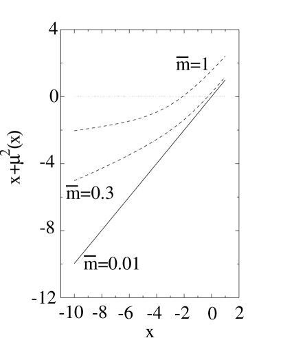
Fig. 6.6: A plot illustrating the $\overline{m}$-dependence of the zero of the propagator denominator in the {$Z,M$} representation for $S(p)$.

In Fig. 6.6 we have plotted $[x+\mu^{2}(x)]$ for a range of values of $\overline{m}$. The striking observation is that this has a $\overline{m}$ dependent zero. A pole in the propagator is only avoided, therefore, because $\zeta(x)$ also has a zero at this point, Eq. (6.73); i.e., $\zeta$ and $x+\mu^{2}$ have coincident zeros. [We remark that a zero in $\zeta$ with $\mu$ finite entails a pole in the functions $A(x)$ and $B(x)$ of Eq. (6.41).]

To summarise: In the first model [the bare vertex] we see that $M(p^{2})$ diverges in the timelike region [Euclidean $p^{2}<0$] so that a pole in the quark propagator is avoided and hence the theory is confining. In the second model [the CP or BC vertex] for $m=0$ there is confinement [the quark propagator is entire] and the phase with no DCSB [i.e., with $M(p^{2})=0$] is energetically favoured. When $m\neq 0$ in the second model we find DCSB and that confinement occurs through cancelling zeros in the numerator and denominator of the quark propagator. It is interesting to speculate that the effective gluon propagator is primarily responsible for confinement and that the vertex modifies the particular manifestation for the quark propagator. However, other models need to be studied before any such conclusion can be drawn.

Application of a Confinement Test.       The confining models discussed above could be studied in the timelike region because their simple form allowed them to be written as coupled differential equations. In the general case an integral equation must be solved and the extension into the timelike region is highly nontrivial. It is still possible to probe the timelike behaviour of the quark propagator obtained by numerical solution of a model quark DSE. In order to determine whether the quark propagator obtained as a solution to our DSE can represent a confined particle we follow Hollenberg et al. (1992) and adapt a method commonly used in lattice QCD to estimate bound state masses. We write as before

$$\sigma_{S}(p^{2})=\frac{B(p^{2})}{p^{2}A(p^{2})^{2}+B(p^{2})^{2}}$$ (6.74)

and define

$$\Delta_{S}(T,\vec{x})=\int\,\frac{d^{4}p}{(2\pi)^{4}}{\rm e}^{i(p_{4}T+\vec{p}\cdot\vec{x})}\sigma_{S}(p^{2})~{}.$$ (6.75)

This is the scalar part of the Schwinger function of the model quark propagator. If we now define

$$\Delta_{S}(T)=\int\,d^{3}x\,\Delta_{S}(T,\vec{x})$$ (6.76)

and, for notational convenience, $E(T)=-\ln\left[\Delta_{S}(T)\right]$, then it follows that if there is a stable asymptotic state with the quantum numbers of this Schwinger function then

$$\lim_{T\rightarrow\infty}\frac{dE(T)}{dT}\,=m~{};$$ (6.77)

where $m\geq 0$ is the asymptotic [on-shell] mass of this excitation; i.e., this limit yields the dynamically generated quark mass evaluated at the mass pole. If the limit in Eq. (6.77) exists for a given propagator then we can conclude that the propagator has a timelike mass pole, which suggests that the associated excitation is not confined.

For example, one can consider the model of Burden et al. (1992b) discussed above and one finds

$$\frac{dE(T)}{dT}\stackrel{{\scriptstyle T\rightarrow\infty}}{{\sim}}\kappa T$$ (6.78)

where $\kappa$ is a constant and hence the limit in Eq. (6.77) does not exist. In this case the Schwinger function does not satisfy the cluster decomposition property and hence the quarks are confined (Roberts et al., 1992). Alternatively one may say that through self interaction the quark acquires an infinite dynamical-mass. This provides another way of understanding the claim that the model of Burden et al. (1992b) is confining.

Another example of this approach is to apply it to the IR vanishing gluon propagator of Eq. (6.29). We set $\alpha_{s}$ to a constant here for simplicity and then, for the boson analogue of $\Delta_{S}(T)$, one finds:

$$\Delta(T)\propto\frac{1}{b\surd 2}\exp\left(-\frac{b\,T}{\surd 2}\right)\left(\cos\left(\frac{b\,T}{\surd 2}\right)-\sin\left(\frac{b\,T}{\surd 2}\right)\right)~{}.$$ (6.79)

Note that the Schwinger function in this case is not positive definite, which is an easily identifiable signal in $\Delta(T)$ due to the pair of complex conjugate poles. This violates the axiom of reflection positivity. It follows from this that Eq. (6.79) describes a field with a complex mass spectrum and/or residues that are not positive. This is appropriate for particles that decay and forms the basis of the argument that such a propagator allows coloured states to exist only for a finite time [of the order of $1/b$] before hadronising; i.e., that the propagator describes confined gluons (Stingl, 1986; Häbel et al. 1990a, 1990b; Zwanziger, 1991).

To illustrate this procedure for an explicit numerical solution we return to the example of the model quark DSE discussed in Sec. 6.2 and attempt to determine whether the model gluon propagator specified by Eqs. (6.28) and (6.29) leads to quark confinement; i.e., the absence of free quarks in the QCD spectrum (Hawes et al. (1993). In applying this method here it is obvious that numerical evaluation of the Fourier transforms required in using Eq. (6.77) will be hindered by numerical noise as $T$ is increased. In order to minimise the effect of this noise on the derivative, we fitted $\Delta_{S}(T)$ to a form

$$C\exp\left(-mT\right)$$ (6.80)

and extracted the derivative from this fit. [Importantly, there is no indication in the results of the structure suggested by Eq. (6.79).] This was particularly useful with the propagators obtained using small values of $b$ which had large dynamical masses [as one would expect since the condensate is large in this case] and hence a rapid decline with $T$. Results were found for the confinement test in the following cases: 1) The propagators obtained with $\ln\tau=0.1$ and $b^{2}$ in the range $[0.1,1.0]$; 2) The propagator obtained with $\ln\tau=0$ and $b^{2}=0.35$ which yields the largest value of $-\langle\overline{q}q\rangle_{\mu}$ on the $(b^{2},\ln\tau)$ domain considered; 3) Two propagators obtained with $(b^{2},\ln\tau)=(0.1,0.6)$ - one using the Ball-Chiu vertex and another using the Curtis-Pennington addition. The results obtained by fitting the form Eq. (6.80) to our numerical output are presented in Table. 6.2.

Table 6.2: Asymptotic dressed-quark-mass values for the family of propagators with $\ln\tau=0.1$, the propagator which showed maximal DCSB (at $\ln\tau=0$ and $b^{2}=0.35$), and for $\ln\tau=0.6$, $b^{2}=0.1$ with both the Ball-Chiu and Curtis-Pennington vertices. These values were arrived at by exponential fit and match the limits of the asymptotic mass curves.

$\ln\tau$	$b^{2}$	$m_{\rm free}$	$C$	Comments
.1	.25	0.410	0.664	B-C vertex
.1	.35	0.296	0.633	”
.1	.45	0.176	0.619	”
.1	.54	0.0275	0.619	”
.0	.35	0.406	0.667	”
.6	0.1	0.210	0.648	B-C vertex
.6	0.1	0.210	0.507	C-P vertex

Fig. 6.7: Dressed-quark-mass curves for the family of propagators with the minimal Ball-Chiu vertex and $\ln\tau=0.1$. The masses are in units of $\Lambda_{\rm QCD}.$

In Fig. 6.7 we present plots of $E^{\prime}(T)$ for the family of propagators obtained with $\ln\tau=0.1$ and this clearly illustrates that an unambiguous determination of the dressed-quark-mass is possible. It will be observed that the mass decreases with increasing $b^{2}$. This is easily understood in terms of the chiral phase transition: as $b$ increases beyond $b_{c}$ there is no DCSB and massless current quarks remain massless. Since the behaviour of all the other solutions we obtained was qualitatively the same as that described by the results presented in Table 6.2 and Fig. 6.7 we infer that the model considered here does not yield a confining quark propagator. We also note that the rainbow approximation studies of the fermion DSE in Alkofer and Bender (1993), which address the question of confinement by a direct continuation to Minkowski momentum space, found a quark propagator with a pole at timelike $p^{2}$; i.e., a non-confining propagator. We remark that, within numerical noise, the Curtis-Pennington addition made no difference to the dressed-quark-mass value extracted in the cases considered and only slightly reduced the normalisation constant $C$. Clearly, the Curtis-Pennington addition leads only to a minor quantitative effect in this part of our study too.

It is worthwhile to recall the suggestion [Häbel et al. (1990a,b)] that a model gluon propagator with the infrared form of Eq. (6.29) would lead to a confining quark propagator of the form

$$\frac{i\gamma\cdot p+c_{0}}{(i\gamma\cdot p+c_{1})\,(i\gamma\cdot p+c_{1}^{\ast})}$$ (6.81)

where $c_{0}$ and $c_{1}$ are real and complex constants, respectively; i.e., to a fermion propagator with complex conjugate poles just as the gluon propagator has; confinement being realised through the absence of poles on the real timelike axis. As Eq. (6.79) shows, such a propagator has a characteristic signature in $\Delta_{S}(T)$ which we do not see in Fig. 6.7. In this model then it is clear that a fermion propagator of the type in Eq. (6.81) does not arise. This does not eliminate the possibility that it can arise in the approach of Häbel et al. (1990a, 1990b), however, since the rational-polynomial Ansätze employed for the vertex functions therein leads to a completely different quark-gluon vertex to that used here. The above results do however suggest that a fermion propagator of the type in Eq. (6.81) cannot arise if the quark-gluon vertex is free of kinematic singularities.

6.3 Euclidean $\leftrightarrow$ Minkowski Continuation

We have discussed this issue in Sec. 2.3 and here we simply put these earlier remarks into context by way of a few examples.

The model of Eqs. (6.43) and (6.44) yields a quark propagator which has complex conjugate branch points with spacelike real parts. Clearly, therefore, the naive transcription rules of Sec. 2.3 will not be suitable in this case. In the modification of this model, Eqs. (6.5) and (6.43), one obtains a quark propagator that is an entire function with an essential singularity at timelike infinity. In this case it is not possible to close the integration contour and hence a “Wick rotation” is simply not possible. This latter case illustrates that the inability to perform a Wick rotation appears even in models which go beyond the rainbow approximation.

Detailed analyses of the analyticity properties of quark propagators obtained with other model gluon propagators in rainbow approximation have been carried out (Stainsby and Cahill, 1992; Maris and Holties, 1992; Stainsby, 1993, Sec. 3; Maris, 1993, Sec. 3.3). In the studies by Stainsby and Cahill (1992) and Stainsby (1993) three forms of gluon propagator were considered:

$$D_{\mu\nu}(q)=\delta_{\mu\nu}\,\frac{4\pi\alpha(q^{2})}{q^{2}}$$ (6.82)

with [$s=q^{2}$]

$$\alpha_{1}(s) = \frac{3\pi\chi^{2}}{4\Delta^{2}}\,\exp\left(\,-\,\frac{s}{\Delta}\right)+\frac{4\pi}{11\ln\left(1+\epsilon+\frac{s}{\Lambda^{2}_{\rm QCD}}\right)}~{},$$ (6.83)

where $\chi=1.14$ GeV, $\Delta=0.002$ GeV², $\Lambda_{\rm QCD}=0.19$ GeV and $\epsilon=2.0$, taken from Praschifka et al. (1989) where it was shown that such a gluon propagator is well suited to a description of low energy hadronic physics;

$$\alpha_{2}(s)=\frac{C_{1}}{s+s_{0}} \;\;{\rm and}\;\; \alpha_{3}(s)=C_{2}\exp\left(\,-\,\frac{s}{s_{0}^{\prime}}\right)$$ (6.84)

with $C_{1}\approx 1$, $s_{0}\approx(0.0707)^{2}$ GeV² and $C_{2}\approx 50.0$ and $s_{0}^{\prime}\approx(0.245)^{2}$ GeV² chosen so that the solutions obtained for $A(p^{2})$ and $B(p^{2})$, with $p^{2}$ on the real spacelike axis, were very similar to those found with $\alpha_{1}$. Solving the integral equations directly, with no approximation of the kernel, it was found that in each case there were pairs of complex-conjugate, logarithmic branch points with spacelike real part in the functions $A(p^{2})$ and $B(p^{2})$ and hence in the quark propagator. The position of the branch point depended on the form of the propagator but not its nature or existence:

$$\begin{array}[]{ccc}\alpha_{1}:s_{B}\approx 0.22+0.25\,i~{},&\alpha_{2}:s_{B}\approx 0.015+0.33\,i~{},&\alpha_{3}:s_{B}\approx 0.06+0.41\,i~{}.\end{array}$$ (6.85)

Maris (1993) considered two model forms of gluon propagator

$$D_{\mu\nu}(q)=\left(\delta_{\mu\nu}-\frac{q_{\mu}q_{\nu}}{q^{2}}\right)\,\frac{4\pi\alpha(q^{2})}{q^{2}}$$ (6.86)

with

$$\alpha_{1}(q^{2})=\frac{d_{M}\pi}{\ln\left(\tau+\frac{q^{2}}{\Lambda_{\rm QCD}^{2}}\right)}\; \;\;{\rm and}\;\; \;\frac{4\pi\alpha_{2}(q^{2})}{q^{2}}=\eta^{2}\delta^{4}(q)+\frac{4\pi\alpha_{1}(q^{2})}{q^{2}}~{}.$$ (6.87)

The first form is a simple extension of the one loop renormalisation group result for the running coupling in QCD to small-$q^{2}$ and the second form involves an additional “confining term”, $\delta^{4}(q)$. The DSEs obtained were analysed using the approximation of Eq. (4.7) to obtain differential equations.

In the case of $\alpha_{1}$ there are five singularities, two of which are simply those of the running coupling; i.e., at $x=-\tau$ and $x=-\tau+1$, where $x=p^{2}/\Lambda_{\rm QCD}^{2}$, and can therefore be discarded as artifacts of the model. Of the three not trivial singularities, two are complex conjugate branch points and one is a branch point on the timelike $p^{2}$ axis with $-\tau+1<x_{B}<0$. This latter singularity might be used to define the quark mass shell.

The singularity structure of the $\alpha_{2}$ model is interesting and complicated. The most interesting feature is that the singularity on the timelike axis bifurcates into a pair of complex conjugate branch points in the presence of the “confining” term thereby eliminating the quark mass shell. In addition, the branch points that were present with $\alpha_{1}$ alone also bifurcate and move as $\eta^{2}$ is changed.

In each of these examples the naive Wick rotation, given by the transcription rules of Eqs. (2.83), (2.84) and (2.85), does not yield the correct continuation of the Euclidean space DSE to Minkowski space. This serves to emphasise the points we made in the last subsection of Sec. 2.3.

7 Applications to Hadron Structure

In this section we will apply the knowledge harvested from the studies of the DSEs in QCD, all of which is necessary, to the study of the kinematic and dynamical properties of hadrons. We will work for the most part in Euclidean space.

7.1 Coupled Dyson-Schwinger and Bethe-Salpeter equation Phenomenology

One direct application of the tower of DSEs to hadron phenomenology is to solve the bound state equations using a kernel constructed from the dressed quark and gluon propagators discussed above. In Fig. 7.1 we illustrate the BSE for mesons. We are assuming non-flavour-singlet mesons and so only the homogeneous BSE is shown. In this figure we employ the convention that $i\chi=S\Gamma_{\rm meson}S$ and the BSE quark-anti-quark kernel is $K=(i\Gamma)(iD)(i\Gamma)+\cdots$. Retaining only the first term shown for $K$ yields the dressed-ladder approximation for the BSE.

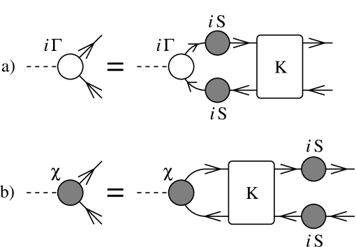
Fig. 7.1: Shown are two equivalent forms of the BSE; i.e., (a) the proper meson-quark vertex [$\Gamma_{\rm meson}$] and (b) the Bethe-Salpeter amplitude for the meson [$i\chi=S\Gamma_{\rm meson}S$].

There have been a number of studies of the covariant BSE for mesons using a kernel constructed from a model dressed gluon propagator, whose ultraviolet behaviour is fixed by the QCD renormalisation group and whose infrared behaviour is based on the studies described in Sec. 5.1, and a dressed quark propagator obtained as a solution of the rainbow approximation DSE with the same model gluon propagator. In a series of studies (Cahill et al., 1987; Praschifka, 1988; Praschifka et al., 1989; Stainsby, 1993, Sec. 4; Stainsby and Cahill, 1993) it was shown that this system of equations provides a very good description of the $u$- and $d$-quark sector of the mesonic spectrum with the choice

$$D_{\mu\nu}(q)=\delta_{\mu\nu}\left(C\,\Lambda_{\rm QCD}^{2}\,\delta^{4}(q)+\frac{d_{M}\pi}{q^{2}\,\ln\left(\tau+\frac{q^{2}}{\Lambda_{\rm QCD}^{2}}\right)}\right)$$ (7.1)

with $C=(3\pi)^{3}$ and $\tau=3$. These model studies incorporated quark confinement in the sense discussed in Sec. 6.2 and will be discussed further in Sec. 7.2.

In addition, there have been phenomenologically successful studies of this coupled system using an infrared-finite form of the model gluon propagator subject to the approximation of Eq. (4.7) (Dai et al., 1991; Aoki et al., 1991) and noncovariant, Coulomb-gauge studies of a pion BSE whose kernel is constructed using a dressed quark propagator obtained as a solution of the Coulomb-gauge quark-DSE with a bare gluon propagator (Govaerts et al., 1984) and a model dressed gluon propagator which is singular in the infrared (Alkofer and Amundsen, 1988).

We cannot summarise all of these studies and choose instead to discuss, as a particular example, recent studies by Munczek and Jain (1992) and Jain and Munczek (1993) which consider pseudoscalar- and vector-$q$-$\overline{q}$ bound states of $u$-, $d$-, $s$-, $c$- and $b$-quarks. The treatment necessarily used significant approximations and was carried out in Euclidean space, which required extrapolation into the timelike region in order to extract the meson masses. The second of these articles is somewhat simpler and more systematic and we summarise its arguments and results here. It is important to note that solving the BSE with a kernel that is consistent with the solution of the quark DSE is necessary to guarantee the Goldstone-boson nature of the pion in the chiral limit (Delbourgo and Scadron, 1979).

As in the studies summarised briefly above, the principal initial approximation in this model is that the quark-gluon vertex is simply given by $\Gamma_{\mu}=\gamma_{\mu}$ and the $q-\bar{q}$ scattering kernel is given by an effective single-gluon propagator. This is a ladder-type approximation with a modified gluon propagator $D_{\mu\nu}$. In this approximation, the BSE for a $q\bar{q}$ bound state of mass $m^{2}_{fg}=p^{2}$ can be written in Minkowski space as,

$$(S^{f})^{-1}(q+\alpha p)\chi(p,q)(S^{g})^{-1}(q-\beta p)={16\pi\over 3}i\int{d^{4}k\over(2\pi)^{4}}\gamma_{\mu}\chi(p,k)\gamma_{\nu}D^{\mu\nu}(k-q)\ ,$$ (7.2)

with $\alpha+\beta=1$. The quark propagators are obtained by solving the DSE for a fermion flavor $f$, in the rainbow approximation,

$$(S^{f})^{-1}(q)=\mbox{$\not\!q$}-m_{f}-i{16\pi\over 3}\int{d^{4}k\over(2\pi)^{4}}\gamma_{\mu}S^{f}(k)\gamma_{\nu}D^{\mu\nu}(k-q)\;.$$ (7.3)

Note that for convenience $\alpha_{s}(-(k-q)^{2})$ has been absorbed into the definition of the effective gluon propagator here [as in Jain and Munczek (1993)]. The Euclidean space form of these equations is [see Secs. 2.3 and 6.3]:

$$(S^{f})^{-1}(q+\alpha p)\chi(p,q)(S^{g})^{-1}(q-\beta p)=-{16\pi\over 3}\int{d^{4}k\over(2\pi)^{4}}\gamma_{\mu}\chi(p,k)\gamma_{\nu}D_{\mu\nu}(k-q)~{},$$ (7.4)

$$(S^{f})^{-1}(q)=i\gamma\cdot q+m_{f}+{16\pi\over 3}\int{d^{4}k\over(2\pi)^{4}}\gamma_{\mu}S^{f}(k)\gamma_{\nu}D_{\mu\nu}(k-q)\ .$$ (7.5)

The ladder-rainbow approximation has been argued to be most appropriate in Landau gauge (Fomin et al., 1983; Atkinson et al., 1988c) in which case the model dressed gluon propagator can be written

$$D_{\mu\nu}(k)=\bigg{(}\delta_{\mu\nu}-{k_{\mu}k_{\nu}\over k^{2}}\bigg{)}D(k^{2})~{}.$$ (7.6)

Jain and Munczek (1993) choose the momentum dependence of the gluon propagator taken to be

$$D(k^{2})=\bigg{[}{d_{M}\pi\over k^{2}\ln(\tau+x)}\bigg{(}1+b{\ln[\ln(\tau+x)]\over\ln(\tau+x)}\bigg{)}\bigg{]}+D_{IR}(k^{2})\;,$$ (7.7)

where $x\equiv k^{2}/\Lambda_{\rm QCD}^{2}$ and $\Lambda_{\rm QCD}\simeq 200$MeV is the QCD scale parameter. In Eq. (7.7), $d_{M}\!=12/[33-2N_{f}]$, $b=2\beta_{2}/\beta_{1}^{2}$, $\beta_{1}=N_{f}/3-11/2$, $\beta_{2}=19N_{f}/12-51/4$ and $N_{f}$ is the number of quark flavors, [taken as five in these calculations] and so, at large $k^{2}$, the expression in parentheses agrees with the two-loop renormalisation group result for the running coupling in QCD, Eq. (5.9). As in many of the studies described above, the parameter $\tau$ regulates the infrared behaviour of the running coupling. As long as its value is larger than $\sim 2$, the results of the calculations are largely insensitive to it. The value adopted by Jain and Munczek is $\tau=10$.

The infrared effects in the model are dominated by $D_{IR}(k^{2})$, which for simplicity was taken to have a modified Gaussian form

$$D_{IR}(k^{2})=\pi a\ k^{2}\ e^{-\mu k^{2}}\ ,$$ (7.8)

with $a=(0.387\ GeV)^{-4}$ and $\mu=(0.510\ GeV)^{-2}$. Defining the classical potential by analogue with Eq. (3.5), including the negative sign associated with attraction and multiplying by the factor $16\pi/3$, this form corresponds to

$$V(r)=\frac{a}{6\mu^{3}}\,\sqrt{\frac{\pi}{\mu}}\,(r^{2}-6\mu)\exp\left(\frac{r^{2}}{4\mu}\right)$$ (7.9)

which is approximately linear out to 0.4 fm. We note that Eq. (7.8) does not incorporate the infrared singularity $\sim\delta^{4}(k)$ that was associated with quark confinement in Sec. 6.2. This term was included in the earlier study by Munczek and Jain (1992).

The most general decomposition for the vector, pseudoscalar and scalar bound state wave functions can be written as

$$\chi_{{}_{V}}(p,q) = i\gamma\cdot\epsilon\,\chi_{{}_{V0}}-i\gamma\cdot p\,\epsilon\cdot q\,\chi_{{}_{V1}}-i\gamma\cdot q\,\epsilon\cdot q\,\chi_{{}_{V2}}+\epsilon\cdot q\,\chi_{{}_{V3}}$$ (7.10)

$$+ [\gamma\cdot\epsilon,\gamma\cdot p]\,\chi_{{}_{V4}}+[\gamma\cdot\epsilon,\gamma\cdot q]\,\chi_{{}_{V5}}-[\gamma\cdot p,\gamma\cdot q]\,\epsilon\cdot q\,\chi_{{}_{V6}}+i\gamma_{5}\gamma\cdot t\,\chi_{{}_{V7}}$$

with $t_{\mu}=\epsilon_{\mu\nu\alpha\beta}q_{\nu}p_{\alpha}\epsilon_{\beta}$, $\epsilon^{2}=-1$ and $\epsilon\cdot p=0$;

$$\chi_{{}_{P}}(p,q)=\gamma_{5}\bigg{[}\chi_{{}_{P0}}-i\gamma\cdot p\,\chi_{{}_{P1}}-i\gamma\cdot q\,\chi_{{}_{P2}}-[\gamma\cdot p,\gamma\cdot q]\,\chi_{{}_{P3}}\bigg{]}~{};$$ (7.11)

$$\chi_{{}_{S}}(p,q)=\chi_{{}_{S0}}-i\gamma\cdot p\,\chi_{{}_{S1}}-i\gamma\cdot q\,\chi_{{}_{S2}}-[\gamma\cdot p,\gamma\cdot q]\,\chi_{{}_{S3}}~{}.$$ (7.12)

In these equations, flavor indices are implicit on $\chi_{{}_{Vi}}$, $\chi_{{}_{Pi}}$ and $\chi_{{}_{Si}}$, which are functions of $p^{2}$, $q^{2}$ and $p\cdot q$.

An important result in this study is that the dominant contributions to the vector and pseudoscalar wave functions is provided by $\chi_{{}_{J0}}^{(0)}$. The BSEs for the dominant wave functions, $\chi_{{}_{J0}}$, are:

$$\chi_{{}_{V0}}(p^{2},q^{2},p\cdot q)={1\over A_{a}A_{b}D}\{(q^{2}-\alpha\beta p^{2}+m_{a}m_{b})+q\cdot p(\alpha-\beta)\}I_{V0}\ +\Delta\chi_{{}_{V0}},$$ (7.13)

with

$$I_{V0}=\int{d^{4}k\over(2\pi)^{4}}\,D(k-q)\chi_{{}_{V0}}\bigg{\{}1+{2\over 3}\bigg{(}1-{q\cdot(k-q)^{2}\over q^{2}(k-q)^{2}}\bigg{)}\bigg{\}}~{};$$ (7.14)

$$\chi_{{}_{P0}}(p^{2},q^{2},p\cdot q)={3\over A_{a}A_{b}D}\{(q^{2}-\alpha\beta p^{2}+m_{a}m_{b})+(\alpha-\beta)q\cdot p\}I_{P0}+\Delta\chi_{{}_{P0}}\ ,$$ (7.15)

with

$$I_{P0}=\int{d^{4}k\over(2\pi)^{4}}\,D(k-q)\chi_{{}_{P0}}~{};$$ (7.16)

$$\chi_{{}_{S0}}(p^{2},q^{2},p\cdot q)={3\over A_{a}A_{b}D}\{(q^{2}-\alpha\beta p^{2}-m_{a}m_{b})+(\alpha-\beta)q\cdot p\}I_{S0}+\Delta\chi_{{}_{S0}}\ ,$$ (7.17)

with

$$I_{S0}=\int{d^{4}k\over(2\pi)^{4}}\,D(k-q)\chi_{{}_{S0}}~{};$$ (7.18)

and where

$$\begin{array}[]{cccc}A_{a}=A_{a}(q+\alpha p)~{},&A_{b}=A_{b}(q-\beta p)~{},&\displaystyle m_{a}={B_{a}(q+\alpha p)\over A_{a}(q+\alpha p)}~{},&\displaystyle m_{b}={B_{b}(q-\beta p)\over A_{b}(q-\beta p)}\end{array}$$ (7.19)

and $D=[(q+\alpha p)^{2}+m_{a}^{2}][(q-\beta p^{2})+m_{b}^{2}]$.

In these equations the $\Delta\chi_{{}_{J0}}$ contain contributions from several of the wave functions $\chi_{{}_{Ji}}$. The technique adopted by Jain and Munczek (1993) to solve these equations was to write $p\cdot q=pq\cos\theta$ and expand the functions $\chi_{{}_{Ji}}$ in terms of Tschebyshev polynomials, $T^{(n)}(\cos\theta)$:

$$\chi_{{}_{Ji}}\biggl{(}q^{2},M_{B}^{2},\cos\theta\biggr{)}=\sum\limits_{n}\,\chi_{{}_{Ji}}^{(n)}\biggl{(}q^{2},M_{B}^{2}\biggr{)}\,T^{(n)}(\cos\theta)~{},$$ (7.20)

where the subscript $J$ ranges over $V$, $P$ and $S$ and $i=1,2,\ldots$ over the independent wave functions. The equation was then projected with the zeroth order Tschebyshev polynomial and the right-hand-side approximated by keeping only the leading order term in the Tschebyshev expansion for $\chi_{{}_{Ji}}$, $i\geq 1$, and by retaining the three lowest terms, $\chi_{{}_{J0}}^{(0)}$, $\chi_{{}_{J0}}^{(1)}$ and $\chi_{{}_{J0}}^{(2)}$, for $\chi_{{}_{J0}}$.

The vector and pseudoscalar meson equations were reduced to single equations for $\chi_{J0}^{(0)}$ by neglecting all contributions on the right-hand-side of the equations for $\chi_{{}_{J0}}^{(1)}$, $\chi_{{}_{J0}}^{(2)}$ and $\chi_{J\,i\geq 1}^{(0)}$ other than the one involving $\chi_{J0}^{(0)}$, thus breaking the self-consistency of the tower of equations that couple the Tschebyshev moments. In the scalar meson case, however, the contribution due to $\chi_{{}_{S2}}^{(0)}$ was found to be important. Consequently the procedure used in the vector and pseudoscalar case was adapted in order to obtain a pair of coupled equations for $\chi_{{}_{S0}}^{(0)}$ and $\chi_{{}_{S2}}^{(0)}$ which were solved self consistently.

In arriving at the final equations to be studied Jain and Munczek (1993) also employed the approximation of expanding the mass functions, $m_{a}$ and $m_{b}$, and the functions $A$ and $B$ in a Taylor series around $q^{2}+\alpha^{2}p^{2}$ or $q^{2}+\beta^{2}p^{2}$, depending on their argument, retaining up to first derivative terms whose contribution to the calculated meson masses was less than 10-15% . Where necessary the solutions for $A$ and $B$, obtained on the spacelike real axis from the quark DSE, were extrapolated to timelike values of their arguments. Electromagnetic effects were incorporated by including the one photon exchange kernel in the BSE and, in order ensure that Goldstone’s theorem remained valid, in the quark DSE. Isospin mass splittings were included by using different masses for the $u$- and $d$- quarks. The projected BSEs were then solved numerically for bound-state mass-eigenvalues and wave functions. The total mass difference between states of the type $q\bar{u}$ and $q\bar{d}$, where $q$ can be any one of the quarks, was obtained as a sum of the isospin and electromagnetic mass splittings except in the case of the pion for which it was assumed that the pure isospin contribution to the mass difference between $\pi^{0}$ and $\pi^{+}$ is negligible.

Table 7.1: Calculated pseudoscalar and vector meson masses and pseudoscalar decay constants obtained by Jain and Munczek (1993) using renormalisation group invariant quark masses of $\hat{m}_{u}=8.73\;{\rm MeV}\;=\hat{m}_{d}$, $\hat{m}_{s}=203$ MeV; “constituent-quark” masses of $M_{c}=1.54$ GeV and $M_{b}=4.74$ GeV, defined as the value of the mass function at $q^{2}=0$, and the values of $a$ and $\mu$ given after Eq. (7.8). These tables were adapted from Jain and Munczek (1993).

meson	$\pi$	$K^{+}$	$s\bar{s}$	$\eta_{c}$	$D_{s}$	$D_{0}$	$\eta_{B}$	$B_{c}$	$B_{s}$	$B_{+}$
mass (MeV)	135	494		2979	1969	1865				5279
(exp.)
mass (MeV)	135	494	703	2821	1872	1756	9322	6126	5249	5149
$f_{M}$ (MeV)	93	114		213	148	125	287	207	119	119
$\alpha$	0.5	0.35	0.5	0.5	0.25	0.2	0.5	0.27	0.10	.09
meson	$\rho$	$K^{*+}$	$\phi$	J/$\psi$	$D_{s}^{*}$	$D_{0}^{*}$	$\Upsilon$	$B_{c}^{*}$	$B_{s}^{*}$	$B_{+}^{*}$
mass (MeV)	770	892	1019	3097	2110	2007	9460			5325
(exp.)
mass (MeV)	760	976	1184	3100	2187	1997	9460	6277	5415	5290
$\alpha$	0.5	0.65	0.5	0.5	0.3	0.3	0.5	0.2	.1	0.07

There are a number of important conclusions: 1) The contribution to a given meson mass due to $\chi_{J\,i\geq 1}$ is negligible in all cases as was the contribution of all Tschebyshev moments of order greater than zero. The net contribution being less than $10$%; 2) There was some dependence of the meson mass on $\alpha$, the relative-momentum distribution parameter, but in all cases it was less than $15$%. In quoting results the authors settled on a value of $\alpha$ for which the response of the mass to changes in $\alpha$ was minimised; 3) The hyperfine splitting was in general too large but the splitting between the ground state and radial excitations was in good agreement with experiment. Some of these observations are apparent from Table 7.1.

As remarked by Jain and Munczek (1993), a number of improvements of this study are possible. The fact that the splitting between vector and pseudoscalar mesons is larger than experimentally observed may indicate the need for an effective scalar interaction in the kernel of the BSE. This must be introduced, however, in such a manner as to ensure the preservation of Goldstone’s theorem and hence will entail a modification of the quark DSE. A natural way to proceed in this direction is to go beyond ladder-rainbow approximation, which requires a dressed vertex in the quark DSE.

Simple improvements in methodology are also possible, for example, one might avoid the Tschebyshev expansion, Taylor expansion and extrapolation procedures. In a study of the pion and scalar-diquark BSEs using a quark propagator based on the DSE studies of Burden et al. (1992b), which are summarised in Sec. 6.2, and subject to the approximations

$$\chi_{{}_{P}}\approx\gamma_{5}\,\chi_{{}_{P0}}\; \;\;{\rm and}\;\; \;\chi_{0^{+}}\approx\,\chi_{0^{+}0}~{},$$ (7.21)

Stainsby and Cahill (1993) solved the integral equations directly by matrix inversion on a discrete grid. The fact that the arguments of the quark propagators in the kernel of the BSEs became complex in Euclidean space, since $P^{2}=-M^{2}$ at the solution, did not present a problem because the quark propagators were regular on the complete integration domain as a consequence of the quark confinement mechanism.

This approach can also be applied to baryons using the relativistic Faddeev equations (Cahill et al., 1989; Burden et al., 1989; Cahill, 1992). Such studies are facilitated by, but not founded upon, the observation that the scalar-diquark, $(qq)_{0^{+}}$, acts effectively as a resonance in the two-body subchannel in which case the Faddeev equation can be written in the form

$$\Psi(p;P) = \frac{1}{f^{2}}\int\frac{d^{4}q}{(2\pi)^{4}}\,\Gamma_{0^{+}}(p+\mbox{\small$\frac{1}{2}$}q+\mbox{\small$\frac{2-3\alpha}{2}$}P)\Gamma_{0^{+}}(q+\mbox{\small$\frac{1}{2}$}p+\mbox{\small$\frac{2-3\alpha}{2}$}P)$$

$$\times S([2\alpha-1]P-p-q)\,S([1-\alpha]P+q)\,D_{0^{+}}(\alpha P-q)\,\Psi(q;P)$$

where $f$ is the normalisation, $\Gamma_{0^{+}}$ is the scalar-diquark Bethe-Salpeter amplitude, which, at the same level of approximation, is obtained as the solution of (Cahill et al., 1987)

$$\Gamma_{0^{+}}(p;P)=\int\frac{d^{4}q}{(2\pi)^{4}}\,\frac{4}{3}D_{\mu\nu}(p-q)\,\gamma_{\mu}S(q-\mbox{\small$\frac{1}{2}$}P)\Gamma_{0^{+}}(p;P)S(q+\mbox{\small$\frac{1}{2}$}P)\gamma_{\nu}~{},$$ (7.23)

$S$ is the dressed quark propagator, obtained as the solution its DSE with a model dressed gluon propagator, and $D_{0^{+}}$ is the scalar-diquark propagator, which can be extracted from the $(qq)_{0^{+}}\rightarrow(qq)_{0^{+}}$ scattering matrix. The first study of Eq. (7.1) (Burden et al., 1989) used parametrisations of the quark and scalar-diquark propagators based on DSE studies. These lead to a quark-core contribution to the baryon mass of $\sim 1.2$ GeV. Various studies of the effect of the pion-cloud suggest that this will lead to a $(-200)\,\sim\,(-300)$ MeV contribution and hence this is a good result. However, there was a flaw in this study: the parametrisations of the quark and scalar-diquark propagators introduced unphysical poles into the integration domain, poles which would not be present in the kernel of Eq. (7.1) if confinement is taken into account. Current studies (Cahill, 1993) are addressing this problem.

7.2 Effective Actions and QCD

Coupled BSE-DSE systems such as the ones described above arise naturally in the effective action approach to field theories. Indeed, the coupled DSE-BSE approach and the effective action approach are equivalent; a given effective action serves to specify a certain order of resummation of the Feynman diagrams that contribute to a given DSE. The application of effective actions and their interplay with the DSE tower has been discussed by McKay and Munczek (1989) and reviewed by Haymaker (1991). There are two commonly used effective actions.

CJT Effective Action.       The CJT effective action (Cornwall et al., 1974) which can be written in Euclidean space as:

$$\Gamma^{\rm CJT}[S]={\rm TrLn}\left[S_{0}^{-1}S\right]+{\rm Tr}\left[1-S_{0}^{-1}\,S\right]+V_{2}[S]$$ (7.24)

where $S$ is the dressed fermion propagator, $S_{0}$ is the free fermion propagator and $V_{2}[S]$ is the sum of all two-particle, irreducible vacuum diagrams (Stam, 1985):

$$V_{2}[S]=\mbox{\small$\frac{1}{2}$}\,{\rm Tr}\left[D_{\mu\nu}\,\Pi_{\mu\nu}\right] = \,-\mbox{\small$\frac{1}{2}$}g^{2}\,\int\frac{d^{4}k}{(2\pi)^{4}}\int\frac{d^{4}q}{(2\pi)^{4}}\,D_{\mu\nu}(k-q)\,{\rm tr}\left[\gamma_{\mu}\,S(q)\,\Gamma_{\nu}(q,k)\,S(k)\right]$$ (7.25)

where $D_{\mu\nu}$ is the dressed gluon propagator and $\Gamma_{\nu}$ is the dressed quark-gluon vertex. From Eq. (6.6), one recognises this as

$$= \,-\mbox{\small$\frac{1}{2}$}\int\frac{d^{4}k}{(2\pi)^{4}}\,{\rm tr}\left[\Sigma(k)\,S(k)\right]~{}.$$ (7.26)

It is therefore obvious that the variational equation

$$\frac{\delta}{\delta S}\Gamma^{\rm CJT}[S]=0\; \;\;{\rm leads~{}to}\;\; S^{-1}=S_{0}^{-1}+\Sigma$$ (7.27)

which is the quark DSE.

One can make use of Eq. (7.27) to find that, evaluated at the stationary point,

$$\Gamma^{\rm CJT}[S]={\rm TrLn}\left[S_{0}^{-1}S\right]+\mbox{\small$\frac{1}{2}$}{\rm Tr}\left[1-S_{0}^{-1}\,S\,\right]~{},$$ (7.28)

which was used above in Eq. (6.52).

Auxiliary Field Effective Action.       The “auxiliary field” effective action, $\Gamma^{\rm AF}[\Sigma]$, is best introduced by way of an example since it cannot be written in a closed form. Consider a field theory defined by the generating functional

$${\cal Z}[J]=\frac{1}{\cal N}\int{\cal D}\overline{q}\,{\cal D}q\,\exp\left(-{\cal A}[\overline{q},q]\,+\,\int d^{4}xd^{4}y\,J_{\alpha\beta}(x,y)q_{\alpha}(x)\overline{q}_{\beta}(y)\right)$$ (7.29)

with an action

$${\cal A}[\overline{q},q]=\int d^{4}xd^{4}y\left[\overline{q}_{\alpha}(x)S_{0}^{-1}(x-y)q_{\alpha}(y)-\mbox{\small$\frac{1}{2}$}q_{\alpha}(y)\overline{q}_{\beta}(x)\,{\cal M}_{\beta\gamma}^{\delta\alpha}(x,y)\,q_{\gamma}(x)\overline{q}_{\delta}(y)\right]~{},$$ (7.30)

where ${\cal M}^{\delta\alpha}_{\beta\gamma}(x,y)={\cal M}_{\delta\alpha}^{\beta\gamma}(y,x)$, and normalised such that ${\cal Z}[0]=1$. Equation (7.29) can be rewritten using the Hubbard-Stratonovich transformation to introduce hermitian, bilocal auxiliary fields, $\beta_{\alpha\beta}(x,y)$. One multiplies ${\cal Z}$ by

$$\int\prod_{\alpha\beta}{\cal D}\beta_{\alpha\beta}\,{\rm e}^{-I_{\rm HS}[\beta]-\int d^{4}xd^{4}y\,J_{\alpha\beta}(x,y)\beta_{\alpha\beta}(x,y)}=$$

$$\int\prod_{\alpha\beta}{\cal D}\beta_{\alpha\beta}\,\exp\left(-\int d^{4}xd^{4}y\,\left[\beta_{\alpha\beta}(y,x)\,\mbox{\small$\frac{1}{2}$}\,{\cal M}_{\beta\gamma}^{\delta\alpha}(x,y)\,\beta_{\gamma\delta}(x,y)+J_{\alpha\beta}(x,y)\beta_{\alpha\beta}(x,y)\right]\right)$$

and renormalises; interchanges the order of integration and performs a change of functional-integration variables:

$$\beta_{\alpha\beta}(x,y)\rightarrow\beta_{\alpha\beta}(x,y)+q_{\beta}(x)\overline{q}_{\alpha}(y)$$ (7.32)

which yields a functional integral over the quark fields that is quadratic and hence can be evaluated:

$${\cal Z}[J]=\frac{1}{{\cal N}^{\prime}}\int\prod_{\alpha\beta}{\cal D}\beta_{\alpha\beta}\,\exp\left[-\overline{\cal A}[\beta]-\int d^{4}xd^{4}y\,J_{\alpha\beta}(x,y)\beta_{\alpha\beta}(x,y)\right]$$ (7.33)

where

$$\overline{\cal A}[\beta]=-{\rm TrLn}\left[{\cal G}^{-1}_{\alpha\beta}(x,y)\right]+I_{\rm HS}[\beta]$$ (7.34)

with

$${\cal G}^{-1}_{\alpha\beta}(x,y)\equiv S_{0}^{-1}(x-y)\delta_{\alpha\beta}+\Sigma_{\alpha\beta}(x,y)=S_{0}^{-1}(x-y)\delta_{\alpha\beta}-{\cal M}^{\delta\beta}_{\alpha\gamma}(x,y)\,\beta_{\gamma\delta}(x,y)~{}.$$ (7.35)

The auxiliary field effective action, $\Gamma^{\rm AF}[\beta]$, is obtained from ${\cal Z}$ via a Legendre transformation

$$\Gamma^{\rm AF}[\beta]+\int d^{4}xd^{4}yJ_{\alpha\beta}(x,y)\beta_{\alpha\beta}(x,y)=W^{\rm AF}[J]\equiv\,-\,\ln\left[{\cal Z}[J]\right]~{},$$ (7.36)

with

$$\frac{\delta W^{\rm AF}[J]}{\delta J_{\alpha\beta}(x,y)}=-\beta_{\alpha\beta}(x,y)\; \;\;{\rm and}\;\; \;\frac{\delta\Gamma^{\rm AF}[\beta]}{\delta\beta_{\alpha\beta}(x,y)}=\,J_{\alpha\beta}(x,y)~{},$$ (7.37)

from which it is clear that, at tree level,

$$\Gamma_{\rm AF}[\beta]\approx\overline{\cal A}[\beta]~{}.$$ (7.38)

The stationary point equation

$$\frac{\delta\overline{\cal A}[\beta]}{\delta\beta_{\alpha\beta}(x,y)}=0\; \;\;{\rm yields}\;\; \;\Sigma_{\alpha\beta}(x,y)={\cal M}_{\alpha\gamma}^{\delta\beta}(x,y)\,{\cal G}_{\gamma\delta}(x,y)\,$$ (7.39)

which is simply the Hartree approximation to the DSE for the fermion self energy in this theory. [As an example one might consider the cases of QED₃ and QED₄ , which are obtained with

$${\cal M}_{\beta\gamma}^{\delta\alpha}(x,y)=e^{2}(\gamma_{\mu})_{\beta\gamma}(\gamma_{\nu})_{\delta\alpha}D_{\mu\nu}(x-y)~{},$$ (7.40)

and serve to illustrate this point.] It follows that in Hartree approximation $\Gamma^{\rm CJT}$ and $\Gamma^{\rm AF}_{\rm tree-level}$ have the same stationary point equation and solutions. Indeed, when evaluated at the stationary point, $\Gamma^{\rm AF}_{\rm tree-level}$=$\Gamma^{\rm CJT}$. However, $\Gamma^{\rm AF}_{\rm tree-level}$ is bounded below whereas $\Gamma^{\rm CJT}$ is not (Haymaker, 1991) and so, for many applications, $\Gamma^{\rm AF}_{\rm tree-level}$ is more useful.

QCD Phenomenology using the Auxiliary Field Effective Action.       The generating functional in equation (7.29) is directly applicable to QED₃ and QED₄ since the gauge boson field can be integrated out to yield a quartic four-fermion interaction [see, for example, Roberts and Cahill (1986)]. Here, however, we are interested in its application to QCD. A model field theory that has received a good deal of attention is defined by the action:

$${\cal A}[\overline{q},q] = \int\,d^{4}x\,\overline{q}(x)[\gamma\cdot\partial+M]q(x)+\mbox{\small$\frac{1}{2}$}\int d^{4}x\,d^{4}y\,j_{\mu}^{a}(x)\,g^{2}D_{\mu\nu}(x-y)j_{\nu}^{a}(y)$$ (7.41)

where $M$ is the quark mass matrix, $j_{\mu}^{a}(x)=\overline{q}(x)\frac{\lambda^{a}}{2}\gamma_{\mu}q(x)$ and

$$g^{2}D_{\mu\nu}(x-y)=\int\,\frac{d^{4}k}{(2\pi)^{4}}e^{ik\cdot x}\left(\left[\delta_{\mu\nu}-\frac{k_{\mu}k_{\nu}}{k^{2}}\right]D(k^{2})+\xi\frac{k_{\mu}k_{\nu}}{k^{4}}\right)$$ (7.42)

represents a model quark-quark interaction, realistic constraints on which are discussed in Sec. 5. [We note that a form of the Nambu–Jona-Lasinio model can be obtained by writing $D(k^{2})=$ constant but this does not satisfy the constraints discussed in Sec. 5.] With this current-current interaction one identifies

$${\cal M}_{\beta\gamma}^{\delta\alpha}(x,y)=g^{2}D_{\mu\nu}(x-y)\,I_{\beta_{F}\gamma_{F}}\,(\gamma_{\mu})_{\beta_{D}\gamma_{D}}\,\left(\frac{\lambda^{a}}{2}\right)_{\beta_{C}\gamma_{C}}\,I_{\delta_{F}\alpha_{F}}\,(\gamma_{\nu})_{\delta_{D}\alpha_{D}}\,\left(\frac{\lambda^{a}}{2}\right)_{\delta_{C}\alpha_{C}}\,$$ (7.43)

where $D$, $C$, $F$ refer to Dirac-, colour- and flavour-space, respectively. Although such a model field theory does not include explicit three- or four-gluon vertices, non-Abelian effects can be incorporated through the structure of $D(k^{2})$, as discussed in Sec. 5. Many independent studies can be correlated within this framework; for example, those of McKay and Munczek (1985); Cahill and Roberts (1985); Praschifka et al. (1987a); McKay et al. (1988); Barducci et al. (1988); Haymaker (1991) and references therein. The nature of the truncations and approximations necessary to obtain Eq. (7.41) from QCD is discussed by Cahill and Roberts (1985) and McKay et al. (1988).

As mentioned above, there is a large body of work in this area and we choose to summarise it by way of a discussion of a series of studies using a form of Eq. (7.41) that has come to be called the Global Colour-symmetry Model [GCM] (Roberts and Cahill, 1985) and which use the following form for the model dressed gluon propagator:

$$D(k^{2})=\frac{\alpha_{1}(k^{2})}{k^{2}}$$ (7.44)

with $\alpha_{1}$ given in Eq. (6.83). This form of the model has been used successfully to calculate the kinematic and dynamical properties of mesons and has also been applied to baryons. One ingredient of its success is that it incorporates confinement in the sense of ensuring the absence of quark production thresholds in any Feynman diagram associated with a physical process, a criterion that is discussed in Sec. 6.2. From the point of view of a connection between the GCM and QCD, Landau gauge, $\xi=0$, is the best choice, as we have seen in the DSE studies described above. However, in developing an efficacious phenomenology, a Feynman-like gauge with $D_{\mu\nu}(k)=\delta_{\mu\nu}\alpha_{1}(k^{2})/k^{2}$ can be used without penalty.

The generating functional for the GCM is given by Eqs. (7.29) and (7.41) from which the auxiliary-field effective action, in the form of Eq. (7.33), follows. In making contact with low energy phenomenology in QCD and the tower of DSEs it is useful to express the generating functional in terms of a local functional integral. This can be achieved (Roberts and Cahill, 1987) by writing

$$\beta_{\alpha\beta}(x,y) \equiv B_{\alpha\beta}\left(w=\mbox{\small$\frac{1}{2}$}(x+y),z=x-y\right)$$ (7.45)

$$= \tilde{\Theta}_{\alpha\beta}(z)+\sum_{k}\,\left[\Phi_{\alpha\beta}^{k}\ast\Theta_{\alpha\beta}^{k}\right](w,z)\equiv\tilde{\Theta}_{\alpha\beta}(z)+\sum_{k}\,\int d^{4}u\,\Phi_{\alpha\beta}^{k}(w-u)\,\Theta_{\alpha\beta}^{k}(u,z)~{},$$

where $\{\Theta_{\alpha\beta}^{k}(w,z);k=0,1,\dots\}$ is a complete set of orthogonal functions, to be specified later, and $\{\tilde{\Theta}_{\alpha\beta}(z)\}$ are those solutions of Eq. (7.39) which actually minimise the action: the translationally invariant “vacuum field configuration”. Using Eq. (7.45), the generating functional becomes

$${\cal Z}[J^{\Phi}]=\frac{1}{{\cal N}^{\prime\prime}}\int\prod_{k}\prod_{\alpha\beta}{\cal D}\Phi_{\alpha\beta}^{k}\,\exp\left[-\overline{\cal A}[\Phi]-\int d^{4}w\,\sum_{k}\,J_{\alpha\beta}^{\Phi(w)k}\Phi_{\alpha\beta}^{k}(w)\right]$$ (7.46)

where $\overline{\cal A}[\Phi]$ follows from direct substitution of Eq. (7.45) in Eq. (7.34). It is clear that since the solutions of Eq. (7.39) have been isolated explicitly the lowest order contribution from $\overline{\cal A}[\Phi]$, in an expansion about $\Phi=0$, is of O$(\Phi^{2})$. The stationary point equation in the GCM is obviously the rainbow-ladder approximation to the quark DSE. Clearly then, of all the combinations $(\alpha\beta)$, the only nonzero $\tilde{\Theta}_{\alpha\beta}$ are the isoscalar, colour-singlet, Dirac-vector and Dirac-scalar combinations, which are related to the Fourier transforms of the functions $A(p^{2})$ and $B(p^{2})$, much discussed above. It follows that, in any expansion of $\overline{\cal A}[\Phi]$ about $\Phi=0$, the dressed quark propagator will be an important element.

In Eq. (7.46) particular $(\alpha\beta)$-combinations correspond to local fields with the quantum numbers of $\pi$-mesons, $\rho$-meson, etc., and whose internal structure is described by the associated $\Theta_{\alpha\beta}$-functions. This is most easily demonstrated by way of an example. Considering an expansion in the $(\alpha\beta)$-combination that corresponds to the isovector, colour-singlet, Dirac-pseudoscalar channel; i.e., the $\pi$-meson, one obtains

$$\overline{\cal A}[\vec{\pi}]=-\,{\rm TrLn}\left[S^{-1}(x-y)-g^{2}\,D_{\mu\nu}(x-y)\gamma_{\mu}\frac{\lambda^{a}}{2}\,\left[\pi_{i}^{k}\ast\Theta_{i}^{k}\right]\left(\mbox{\small$\frac{1}{2}$}(x+y),x-y\right)\gamma_{\nu}\frac{\lambda^{a}}{2}\right]+I_{\rm HS}[\vec{\pi}]$$ (7.47)

where $S(x-y)$ is the dressed quark propagator and, with $i,j$ isospin labels,

$$I_{\rm HS}[\vec{\pi}] = \int\frac{d^{4}P}{(2\pi)^{4}}\,\pi_{i}^{k}(P)\,\mbox{\small$\frac{1}{2}$}\,_{\vec{\pi}}{\cal I}_{ij}^{kl}[\Theta](P)\,\pi_{j}^{l}(-P)$$ (7.48)

with

$${}_{\vec{\pi}}{\cal I}_{ij}^{kl}[\Theta](P) = \int\frac{d^{4}q_{1}}{(2\pi)^{4}}\,\frac{d^{4}q_{2}}{(2\pi)^{4}}\,g^{2}\,D_{\mu\nu}(q_{1}-q_{2})\,{\rm tr}\left[\Theta_{i}^{k}(P,q_{1})\,\gamma_{\mu}\frac{\lambda^{a}}{2}\Theta_{j}^{l}(-P,q_{2})\,\gamma_{\nu}\frac{\lambda^{a}}{2}\,\right]~{},$$ (7.49)

where $P$ is the centre-of-mass momentum, which follows from Eqs. (7.2) and (7.43).

At O$(\pi^{2})$, neglecting the constant vacuum energy, one obtains

$$\overline{\cal A}[\vec{\pi}]=\int\frac{d^{4}P}{(2\pi)^{4}}\ \pi_{i}^{k}(P)\,\mbox{\small$\frac{1}{2}$}\,_{\vec{\pi}}\Delta_{ij}^{kl}[\Theta](P)\,\pi_{j}^{l}(-P)\,$$ (7.50)

where

$${}_{\vec{\pi}}\Delta_{ij}^{kl}[\Theta](P)=\,_{\vec{\pi}}{\cal T}_{ij}^{kl}[\Theta](P)+\,_{\vec{\pi}}{\cal I}_{ij}^{kl}[\Theta](P)$$ (7.51)

with

$${}_{\vec{\pi}}{\cal T}_{ij}^{kl}[\Theta](P) = \int\frac{d^{4}k}{(2\pi)^{4}}\,\frac{d^{4}q}{(2\pi)^{4}}\,\frac{d^{4}r}{(2\pi)^{4}}\,g^{2}D_{\mu\nu}(q)\,g^{2}D_{\rho\sigma}(r)$$

$$\times{\rm tr}\left[S(k+\mbox{\small$\frac{1}{2}$}P)\,\gamma_{\mu}\frac{\lambda^{a}}{2}\Theta_{i}^{k}(P,k-q)\,\gamma_{\nu}\frac{\lambda^{a}}{2}\,S(k-\mbox{\small$\frac{1}{2}$}P)\,\gamma_{\rho}\frac{\lambda^{a}}{2}\,\Theta_{j}^{l}(-P,k-r)\,\gamma_{\sigma}\frac{\lambda^{a}}{2}\,\right]~{}.$$

From Eq. (7.50) it is natural to identify ${}_{\vec{\pi}}\Delta_{ij}^{kl}[\Theta](P)$ as the inverse of the matrix propagator for the $\vec{\pi}^{k}$-field and it is clear that, with the functions $\tilde{\Theta}_{\alpha\beta}$ chosen such the action is minimised, ${}_{\vec{\pi}}\Delta_{ij}^{kl}[\Theta](P)$ is non-negative for all $P^{2}>0$.

Until now the functions $\{\Theta^{k}(w,z),k=0,1,\ldots\}$ have not been specified. If one chooses them such that

$${}_{\vec{\pi}}\Delta_{ij}^{kl}[\Theta](P)\;=0~{},\;\;k\neq l\; \;\;{\rm and}\;\; \frac{\delta\;_{\vec{\pi}}\Delta_{ij}^{kk}[\Theta](P)}{\delta\Theta^{k}(-P,q)}=0~{},$$ (7.53)

which entails that the convolution

$$\Gamma_{i}^{k}(P,p)=\int\frac{d^{4}q}{(2\pi)^{4}}\,g^{2}\,D_{\mu\nu}(p-q)\,\gamma_{\mu}\frac{\lambda^{a}}{2}\,\Theta_{i}^{k}(P,q)\gamma_{\nu}\frac{\lambda^{a}}{2}\,$$ (7.54)

satisfies

$$\Gamma_{i}^{k}(P,q)+\int\frac{d^{4}q}{(2\pi)^{4}}\,g^{2}\,D_{\mu\nu}(p-q)\,\gamma_{\mu}\frac{\lambda^{a}}{2}\,S(q+\mbox{\small$\frac{1}{2}$}P)\Gamma_{i}^{k}(P,q)S(q-\mbox{\small$\frac{1}{2}$}P)\,\gamma_{\nu}\frac{\lambda^{a}}{2}\,=0~{},$$ (7.55)

which is the ladder BSE in the GCM, then the local field variables introduced via Eq. (7.45) represent meson fields whose internal structure is described by a ladder-BSE, the kernel of which involves the model dressed gluon propagator and the dressed quark propagator obtained with this gluon propagator via the quark-DSE. The amplitudes $\Gamma^{k}$ can be normalised in the standard fashion (Itzykson and Zuber, 1980, pp. 482-485). With this interpretation of Eq. (7.45) then the superscript $k$ labels excited states in a given channel so, in the present example: $k=0$ represents the $\pi$-meson; $k=1$, its first excited state; etc.

This discussion demonstrates that the tree-level effective action for the GCM describes non-pointlike meson-fields whose internal structure is given by the solution of the coupled rainbow-DSE–ladder-BSE system; i.e., it is the “quark-core” of the hadron. The connection between the auxiliary-field effective action approach and the coupled DSE-BSE approach discussed in Sec. 7.1 is therefore clear. The higher order terms in the tree-level effective action, O$(\pi^{4})$ etc., describe couplings between these quark-core pions and, although only the pion has been discussed explicitly, the approach can be generalised to incorporate other mesons (Praschifka et al., 1987a) and baryons (Cahill et al., 1989).

In order to study low energy properties of QCD it is common to employ a derivative expansion of tree-level effective action, Eq. (7.47). In the GCM one obtains a complete effective action, a small portion of the real part of which we illustrate here:

$$\int d^{4}x\,\left\{\mbox{\small$\frac{1}{2}$}\left(\partial_{\mu}\vec{\pi}\cdot\partial_{\mu}\vec{\pi}+m_{\pi}^{2}\vec{\pi}\cdot\vec{\pi}\right)+\mbox{\small$\frac{1}{2}$}\left(\partial_{\mu}\vec{\rho}_{\nu}\cdot\partial_{\mu}\vec{\rho}_{\nu}-\partial_{\mu}\vec{\rho}_{\mu}\cdot\partial_{\nu}\vec{\rho}_{\nu}+m_{\rho}^{2}\vec{\rho}_{\mu}\cdot\vec{\rho}_{\mu}\right)\right.$$

$$\left.-g_{\rho\pi\pi}\vec{\rho}_{\mu}\cdot\vec{\pi}\times\partial_{\mu}\vec{\pi}+(\kappa,\eta,\omega,a_{1},\ldots)+{\rm tr}\left[\overline{N}\left(\gamma\cdot\partial+m_{N}-\mbox{\small$\frac{i}{\surd{2}}$}m_{N}\gamma_{5}\vec{\tau}\cdot\vec{\pi}\right)N+\ldots\right]\right\}~{}.$$ (7.56)

Although only shown to second order in $\pi$, the constraints placed by chiral symmetry on the nature of pion self-interactions (Roberts et al., 1988; Roberts et al., 1994) and on interactions between the pion and other hadrons (Roberts et al., 1989) are properly represented. The full action also has an imaginary part which contains the Wess-Zumino term, as any realistic model of QCD must (Praschifka et al., 1987a). In following this procedure one obtains the bound state masses by solving the BSE [or Faddeev equation], as discussed above, and all of the couplings between quark-core mesons and baryons as integrals whose integrand contains the dressed quark propagators and Bethe-Salpeter amplitudes.

For example, if one retains only the dominant functions in the Bethe-Salpeter amplitude for the $\pi$- and $\rho$-mesons, as discussed in Sec. 7.1: $\Gamma_{\rho}$ the dominant vector-amplitude and $\Gamma_{\pi}=B$ the dominant pseudoscalar-amplitude; then, writing the dressed quark propagator as $S(p)=-i\gamma\cdot p\sigma_{V}(p)+\sigma_{S}(p)$, one has

$$f_{\pi}^{2} = \!\!\frac{N_{c}}{8\pi^{2}}\int_{0}^{\infty}\,dx\,x\,B^{2}\,\left(\sigma_{V}^{2}-2\left[\sigma_{S}\sigma_{S}^{\prime}+x\sigma_{V}\sigma_{V}^{\prime}\right]-x\left[\sigma_{S}\sigma_{S}^{\prime\prime}-\left(\sigma_{S}^{\prime}\right)^{2}\right]-x^{2}\left[\sigma_{V}\sigma_{V}^{\prime\prime}-\left(\sigma_{V}^{\prime}\right)^{2}\right]\right),$$ (7.57)

which is obtained from the normalisation condition for the pion’s Bethe-Salpeter amplitude in ladder approximation (Alkofer et al., 1993):

$$2f_{\pi}^{2}P_{\mu}=$$

$$N_{c}\,\int\,\frac{d^{4}k}{(2\pi)^{4}}\,{\rm tr}_{D}\left[\overline{\Gamma}_{\pi}(k;P)S(k_{0-})\Gamma_{\pi}(k;-P)\frac{\partial\,S(k_{0+})}{\partial P_{\mu}}+\overline{\Gamma}_{\pi}(k;P)\frac{\partial\,S(k_{0-})}{\partial P_{\mu}}\Gamma_{\pi}(k;-P)S(k_{0+})\right]$$

with $k_{\alpha\beta}=k+\mbox{\small$\frac{1}{2}$}\alpha\,p+\mbox{\small$\frac{1}{2}$}\beta\,q$, and

$$\langle\overline{q}q\rangle_{\mu^{2}} = \frac{N_{c}}{4\pi^{2}}\int_{0}^{\mu^{2}}\,dx\,x\,\sigma_{S}$$ (7.59)

with the result that $m_{\pi}^{2}f_{\pi}^{2}=(m^{u}_{\mu^{2}}+m^{d}_{\mu^{2}})\,\langle\overline{q}q\rangle_{\mu^{2}}$. [Recall that this expression for $f_{\pi}$ differs from that in Eq. (6.27) and that the difference is due to neglecting contributions to the RHS of Eq. (6.26) from $\Gamma_{5}(p^{\prime},p)$, $p^{\prime}\neq p$. When $Z(p^{2})=1$, both forms are the same.] One also finds (Praschifka et al., 1987b)

$$g_{\rho\pi\pi}=\frac{1}{f_{\rho}f_{\pi}^{2}}\frac{N_{c}}{2\pi^{2}}\int_{0}^{\infty}\,ds\,s\,\Gamma_{\rho}(s)\,A(s)\,B(s)\,\frac{B(s)-\mbox{\small$\frac{1}{2}$}\,s\,B^{\prime}(s)}{(s\,A(s)^{2}+B(s)^{2})^{2}}+\mbox{O}(m_{\rho}^{2})~{},$$ (7.60)

with $f_{\rho}$ given by an expression similar to that in Eq. (7.57) and obtained in the same way. [The fact that $\Gamma_{\pi}=B$ is a manifestation of Goldstone’s theorem in this approach, as it also is in the coupled DSE-BSE approach (Delbourgo and Scadron, 1979). This can be seen heuristically by substituting $\Gamma_{k}\propto i\,\tau_{k}\,\gamma_{5}\,E$ in Eq. (7.55) and noting that the equation that results is solved by $E=B$.] Because of the structure of the model dressed gluon propagator, Eq. (7.44), all of these integrals are finite [except for the quark condensate, which diverges as $[\ln\Lambda_{\rm UV}^{2}/\Lambda_{\rm QCD}^{2}]^{d_{\rm M}}$, as it must in a model that is consistent with the ultraviolet constraints imposed by QCD]. The phenomenological success of the GCM is illustrated in Table 7.2.

One can proceed beyond the tree-level effective action and calculate the effect of meson-loops. The introduction of the auxiliary fields, and their subsequent identification with the quark-core; i.e., ladder bound states, via the connection with the BSE, Eq. (7.55), provides a mechanical framework for the systematic ordering and summation of diagrams. As examples we note that the model has been used successfully to calculate the $\omega$-$\rho$ mass splitting induced by $\rho\rightarrow\pi\pi\rightarrow\rho$, $\rho\rightarrow\omega\pi\rightarrow\rho$, $\omega\rightarrow\rho\pi\rightarrow\omega$ and $\omega\rightarrow\pi\pi\pi\rightarrow\omega$ self energy corrections (Hollenberg et al., 1992) and to analyse the contribution of pion loops to the electromagnetic charge radius of the pion (Alkofer et al., 1993), which is found to be an additive correction to $r_{\pi}^{2}$ of $<15$% at $m_{\pi}=0.14$ GeV. Furthermore, recent calculations of the $\omega$-$\rho$ mixing component of the $N$-$N$ potential (Goldman et al., 1992; Krein et al., 1993; Mitchell et al., 1994) also fit neatly within this framework. The important feature of these meson-loop contributions is that they too are finite because the Bethe-Salpeter amplitudes that describe the quark core of the hadrons appear in every integral and provide natural momentum cutoffs, thus ensuring convergence.

Table 7.2: This is an illustrative set of calculated physical quantities, obtained in the GCM using the propagator of Eq. (7.44). Here $m^{\rm qq}$ are effective diquark-masses and $a_{J}^{I}$ are scattering lengths in $\pi$-$\pi$ scattering. The superscripts indicate the reference that a particular result is taken from: 1) Roberts et al. (1988); 2) Roberts et al. (1994); 3) Praschifka et al. (1987a); 4) Praschifka et al. (1989); 5) Hollenberg et al. (1992); 6) Cahill et al. (1987); 7) Cahill (1992).

	Calculated	Experiment
	Massless u,d	(where applicable/known)
m${}_{\pi}\;^{1,2}$	0	(0 if quarks massless)
f${}_{\pi}\;^{2}$	0.091 GeV	0.093 GeV
m${}_{\omega}\;^{3,4}$	0.745	0.783
m${}_{\omega}-\$m${}_{\rho}\;^{5}$	0.030	0.013
$\Gamma_{\rho}\;^{3,4}$	0.232	0.154
m${}_{{\rm f}_{1}}\;^{3,4}$	1.310	1.283
m${}_{{\rm f}_{1}}-\$m${}_{\omega}\;^{3,4}$	0.565	0.500
m${}^{{\rm qq}}_{0^{+}}\;{}^{4,6}$	0.607
m${}^{{\rm qq}}_{1^{+}}\;{}^{4,6}$	1.170
m${}^{{\rm qq}}_{0^{-}}\;{}^{6}$	0.948
m${}^{{\rm qq}}_{1^{-}}\;{}^{6}$	1.950
m${}_{N}\;^{7}$	1.20 $\sim$ 1.30	0.939
$r_{\pi}\;^{1,2}$	0.59 fm	0.66 fm
$a_{0}^{0}\;{}^{2}$	0.17 (dimensionless)	0.20 (dimensionless)
$a_{0}^{2}\;{}^{2}$	-0.048	-0.037
$a_{1}^{1}\;{}^{2}$	0.030	0.038
$a_{2}^{0}\;{}^{2}$	0.0017	0.014
$a_{2}^{2}\;{}^{2}$	-0.0011

This example illustrates the usefulness of the auxiliary-field effective action [or, equivalently, the coupled rainbow-DSE–ladder-BSE] approach to QCD phenomenology. A few parameters [two or three in the studies described in this section] in the model dressed gluon propagator, chosen in order to parametrise the unknown behaviour of the quark-quark interaction in the infrared, are all that is necessary in order to construct a model field theory, with confinement and dynamical chiral symmetry breaking, which provides a good description of low energy hadronic phenomena. Furthermore, the comparison of the calculated results with experimental data allows one to place constraints on the nature of the quark-quark interaction at small-$q^{2}$. This phenomenological success provides considerable incentive to resolve the questions regarding the formulation of the DSEs in QCD.

8 Summary, Conclusions and Outlook

We began with an introduction to the Dyson-Schwinger equation [DSE] formalism with specific reference to QED and to the renormalisation procedure in this framework. It was then relatively straightforward to extend this discussion to QCD. Following this we presented a survey of studies of strong-coupling QED, both because it is an interesting theory in its own right and because it is an ideal pedagogical tool for DSE studies and their application to QCD. We reviewed the DSE studies of the infrared behaviour of the gluon propagator in QCD and its role in phenomenological studies of dynamical chiral symmetry breaking and confinement. Finally, we collected all of this information together and illustrated how it can be used in relativistic bound state calculations using the BSE for mesons and the Faddeev equation for baryons. This information also provides the foundation for the phenomenologically successful effective-action approach to QCD. We illustrated this approach and demonstrated its equivalence, and importance, to the coupled Bethe-Salpeter–Dyson-Schwinger equation studies.

The strengths of the DSE approach to nonperturbative field theory are its manifest covariance and the natural way in which dynamical chiral symmetry breaking can be described. It is also straightforward to build in the correct perturbative limits for QCD because of asymptotic freedom. From the various model studies it is clear that once the scale of one physical parameter; for example, $f_{\pi}$, is fixed by adjusting the infrared behaviour of the quark-quark interaction, then other quantities are automatically of approximately the right magnitude. The fine tuning relies on the details of the models, with very successful descriptions of a broad range of phenomena being possible with only two or three parameters.

While much has been accomplished, it is apparent that much more needs to be done. It is important to develop a better understanding of the detailed way in which confinement is manifested. Since the DSE formalism is not closed at any finite order it will always be important to draw on information gathered from other nonperturbative studies. For example, it would be very helpful if we could learn more about the infrared behaviour of the gluon propagator and the role of ghosts in QCD from lattice gauge theory studies. However, because of present day limitations on lattice studies, this information is currently unavailable but it is an area where cross-fertilisation could provide significant benefits. The results of recent lattice simulations have shown that such information may be available in the not too distant future.

An important question, in field theory in general, and in the DSE approach in particular, is the connection between Euclidean-space and physical Minkowski space. As we demonstrated, a straightforward transcription of the variables in the DSE will almost never be correct. A direct formulation and solution of the DSEs in Minkowski space is one possibility but this is presently prevented by the complete lack of information about the $n$-point functions on the timelike axis at all but very large momenta. At the present time, both lattice and DSE studies are carried out in Euclidean space and the axioms of field theory used to extract values of physical observables. It is not yet clear when or if it will be possible to perform DSE studies directly in Minkowski space.

Appendix A Landau-Khalatnikov Transformations

As we discussed in Sec. 3.7, on any Ansatz for the fermion–gauge-boson vertex in Abelian gauge theories, one would like to impose the constraint that, when used in a DSE, it ensures local gauge covariance of the solutions. The gauge transformation laws which relate the propagators and fermion-gauge-boson vertex in QED to their Landau gauge counterparts were first given by Landau and Khalatnikov (1956) and Fradkin (1956). These rules are most easily specified in coordinate space and we give below the corresponding Euclidean space transformation laws.

In an arbitrary gauge, the photon propagator is modified from its transverse, Landau gauge, form $D_{\mu\nu}(x;0)$ by the addition of a longitudinal piece parameterised by an arbitrary function $\Delta$:

$$D_{\mu\nu}(x;\Delta)=D_{\mu\nu}(x;0)+\partial_{\mu}\partial_{\nu}\Delta(x).$$ (A.1)

The corresponding rule for the fermion propagator is

$$S(x;\Delta)=S(x;0){\rm e}^{e^{2}[\Delta(0)-\Delta(x)]},$$ (A.2)

where $e$ in the exponent is the gauge coupling constant. The rule for the fermion-photon vertex is

$$B_{\mu}(z;x,y|\Delta) = B_{\mu}(z;x,y|0){\rm e}^{e^{2}[\Delta(0)-\Delta(x-y)]}$$ (A.3)

$$+ S(x-y;0){\rm e}^{e^{2}[\Delta(0)-\Delta(x-y)]}\frac{\partial}{\partial z_{\mu}}[\Delta(x-z)-\Delta(z-y)],$$

where $B_{\mu}$ is the non-amputated vertex defined in momentum space in terms of the amputated vertex, $\Gamma_{\mu}$, by

$$B_{\mu}(p,q)=S(p)\Gamma_{\nu}(p,q)S(q)D_{\mu\nu}(p-q).$$ (A.4)

The transformation rule for the partially amputated vertex

$$\Lambda_{\mu}(p,q)=S(p)\Gamma_{\mu}(p,q)S(q)$$ (A.5)

follows from Eqs. (A.1), (A.2) and (A.3) and is simply:

$$\Lambda_{\mu}(z;x,y|\Delta)=\Lambda_{\mu}(z;x,y|0)e^{e^{2}[\Delta(0)-\Delta(x-y)]}.$$ (A.6)

In the usual covariant gauge fixing procedure the photon propagator takes the form

$$D_{\mu\nu}(k;\xi)=\frac{1}{k^{2}[1+\Pi(k^{2})]}\left(\delta_{\mu\nu}-\frac{k_{\mu}k_{\nu}}{k^{2}}\right)+\xi\frac{k_{\mu}k_{\nu}}{k^{4}},$$ (A.7)

which is obtained by taking $\Delta$ in Eq. (A.1) to be

$$\Delta(x)=-\xi\int\frac{d^{\rm d}k}{(2\pi)^{\rm d}}\frac{e^{-ik\cdot x}}{k^{4}}.$$ (A.8)

Within this set of gauges, one finds that in QED₃ the transformation rule for the fermion propagator, Eq. (A.2), becomes

$$S(x;\xi)=S(x;0)e^{-e^{2}\xi\left|x\right|/8\pi}.$$ (A.9)

The free massless propagator is $S^{-1}(p;0)=i\gamma\cdot p$ which corresponds to the following function in configuration space:

$$S(x;0)=\frac{\gamma\cdot x}{4\pi|x|^{3}}.$$ (A.10)

Applying Eq. (A.2) one obtains the LKF transformed function in an arbitrary covariant gauge:

$$S(x;\xi)=\frac{\gamma\cdot x}{4\pi|x|^{3}}e^{-e^{2}\xi\left|x\right|/8\pi}.$$ (A.11)

For $\xi>0$ one may evaluate the Fourier amplitude directly to obtain

$$S(p;\xi)=\frac{-i\gamma\cdot p}{p^{2}}\left[1-\frac{e^{2}\xi}{8\pi p}\arctan\left(\frac{8\pi p}{e^{2}\xi}\right)\right].$$ (A.12)

Appendix B Quark Condensate

We discuss here the meaning of the quark condensate $\langle\bar{q}q\rangle$. It is convenient to perform a Wick rotation and evaluate $\langle\bar{q}q\rangle$ in Euclidean space. Then using

$$\int d^{4}\ell f(\ell^{2})=\pi^{2}\int_{0}^{\infty}d\ell^{2}\ell^{2}f(\ell^{2})$$ (B.1)

we can write Eq. (6.16) as

$$\langle\bar{q}q\rangle=-{3\over 4\pi^{2}}\int^{\Lambda^{2}_{\rm UV}}_{0}d\ell^{2}{\ell^{2}Z(\ell^{2})M(\ell^{2})\over\ell^{2}+M^{2}(\ell^{2})}\;,$$ (B.2)

where we have chosen $\mu=\Lambda_{\rm UV}$ as in Eq. (6.7) and Eq. (6.9) etc. Now, writing an explicit subscript $\Lambda_{\rm UV}$ where appropriate, we have

$$\langle\bar{q}q\rangle_{\Lambda_{\rm UV}}=-{3\over 4\pi^{2}}\int^{\Lambda_{\rm UV}^{2}}_{0}d\ell^{2}\frac{\ell^{2}Z_{\Lambda_{\rm UV}}(\ell^{2})M_{\Lambda_{\rm UV}}(\ell^{2})}{\ell^{2}+M^{2}_{\Lambda_{\rm UV}}(\ell^{2})}\mathrel{\mathop{\simeq}_{\Lambda_{\rm UV}\to\infty}}\ -{3\over 4\pi^{2}}\int^{\Lambda_{\rm UV}^{2}}_{0}d\ell^{2}M_{\Lambda_{\rm UV}}(\ell^{2})~{}.$$ (B.3)

The second result follows since the UV dominates for large $\Lambda_{\rm UV}$ and since in Landau gauge $Z_{\Lambda_{\rm UV}}(\ell^{2})\simeq 1$, for large $\ell^{2}$. In the case of exact chiral symmetry [i.e., $m_{\Lambda_{\rm UV}}=0$] Eq. (6.14) implies that $M_{\Lambda_{\rm UV}}(\ell^{2})=(c/\ell^{2})\ln(\ell^{2}/\Lambda^{2}_{QCD})^{d_{M}-1}$ and hence, from Eq. (B.3), we find

$$\langle\bar{q}q\rangle_{\Lambda_{\rm UV}}\ \mathrel{\mathop{\simeq}_{\Lambda_{\rm UV}\to\infty}}\ -{3\over 4\pi^{2}}\ {c\over d_{M}}\ \left[\ln(\Lambda^{2}_{UV}/\Lambda^{2}_{QCD})\right]^{d_{M}}\;.$$ (B.4)

Since $c$ is independent of the choice of $\mu$ then Eq. (6.14) follows immediately.

We see from Eq. (6.15) that $M_{\Lambda_{\rm UV}}(\ell^{2})\!=\!\hat{m}/[{1\over 2}\ln(\ell^{2}/\Lambda^{2}_{QCD})]^{d_{\rm M}}$ in the presence of an ECSB mass, $m_{\Lambda_{\rm UV}}\!\neq\!0$. It is clear that Eq. (6.17) will no longer result from Eq. (B.3) and so the quark condensate, as defined in Eq. (6.16), no longer varies with the renormalisation point as $\langle\bar{q}q\rangle\sim[\ln(\mu^{2}/\Lambda^{2}_{QCD})]^{d_{M}}$.

Appendix C Pion Decay Constant

We derive the expression for $f^{2}_{\pi}$ given in Eq. (6.27). First note that only terms up to ${\cal O}(k)$ need be kept since we will be taking $k\to 0$. For any function of $p^{2}$, say $f(p^{2})$, we have

$$f((p+k)^{2})=f(p^{2})+2k\cdot p\ {df\over dp^{2}}(p^{2})+{\cal O}(k^{2})\;.$$ (C.1)

In Eq. (6.27) the trace is over isospin, spinor, and colour labels. The spinor trace simplifies things considerably since [in an obvious shorthand notation]

$${\rm tr}\biggl{\{}[S(p) + k\cdot\partial S(p)][\Gamma^{m}_{5}(p,p)+{\cal O}(k)\gamma_{5}][S(p)][(\tau^{n}/2)\gamma^{\sigma}\gamma_{5}]\biggr{\}}$$ (C.2)

$$= {\rm}tr\biggl{\{}k\cdot\partial S(p)\Gamma^{m}_{5}(p,p)S(p)(\tau^{n}/2)\gamma^{\sigma}\gamma_{5}\biggr{\}}+{\cal O}(k^{2})\;,$$

where we have used the fact that ${\rm tr}\left\{S(p)\gamma_{5}S(p)\gamma^{\sigma}\gamma_{5}\right\}=0$, which follows from Dirac matrix algebra, and the assumption that $\Gamma_{5}(p^{\prime},p)=\Gamma_{5}(p,p)+{\cal O}(k)\gamma_{5}$, where the ${\cal O}(k)\gamma_{5}$ term is assumed to have a purely $\gamma_{5}$ spinor structure. Now we can use $\vec{\Gamma}_{5}(p,p)$ which is known from the Goldberger-Treiman relation, Eq. (6.21). We can now use the above results in Eq. (6.26), operate on both sides with $(k_{\sigma}/k^{2})$ and use ${\rm tr}(\tau^{m}\tau^{n})=2\delta^{mn}$ to give

$$f^{2}_{\pi}={3i\over k^{2}}\int{d^{4}p\over(2\pi)^{4}}{\rm tr_{spinor}}\biggl{\{}k\cdot\partial S(p)\gamma_{5}B(p^{2})S(p)A(p^{2})\mbox{$\not\!k$}\gamma_{5}\biggr{\}}$$ (C.3)

where the trace is now over spinor labels only. The factor of three comes from the trace over colour. After evaluating $(\partial/\partial p^{\nu})S(p)$ and taking the spinor trace we find the result of Eq. (6.27). For completeness we also give here the Euclidean-space form of Eq. (6.27), which is

$$f^{2}_{\pi}=\frac{3}{4\pi^{2}}\int_{0}^{\infty}dp^{2}\;{p^{2}Z(p^{2})M(p^{2})\over[p^{2}+M^{2}(p^{2})]^{2}}\left[M(p^{2})-{p^{2}\over 2}{dM\over dp^{2}}\right]\;.$$ (C.4)

References

Alkofer, R. and Amundsen, P.A. (1988). Chiral symmetry breaking in an instantaneous approximation to Coulomb gauge QCD, Nucl. Phys. B, 306, 305.

Alkofer, R. and Bender, A. (1993). Work in progress and private communication.

Alkofer, R., Bender, A. and Roberts, C.D. (1993). Pion loop contribution to the electromagnetic pion charge radius, Argonne National Laboratory Preprint ANL-PHY-7663-TH-93 and Universität Tübingen Preprint UNITUE-THEP-13/1993.

Altarelli, G. (1982). Partons in quantum chromodynamics, Phys. Rep. 81, 1.

Aoki, Ken-Ichi, Kugo, Taichiro and Mitchard, Mark K. (1991). Meson properties from the ladder Bethe-Salpeter equation, Phys. Lett. B 266, 467.

Appelquist, T.W. and Carrazzone, J. (1975). Infrared singularities and massive fields, Phys. Rev. D 11, 2856.

Appelquist, T. and Pisarski, R.D. (1981). High-temperature Yang-Mills theories and three-dimensional quantum chromodynamics, Phys. Rev. D 23, 2305.

Appelquist, T.W., Bowick, M., Karabali, D. and Wijewardhana, L.C.R. (1986). Spontaneous chiral-symmetry breaking in three-dimensional QED, Phys. Rev. D 33, 3704.

Appelquist, T., Nash, D and Wijewardhana, L.C.R. (1988). Critical behaviour in (2+1)-dimensional QED, Phys. Rev. Lett. 60, 2575.

Atkinson, D. and Blatt, D.W.E. (1979). Determination of the singularities of the electron propagator, Nucl. Phys. B 151, 342.

Atkinson, D. and Johnson, P.W., Schoenmaker, W.J. and Slim, H.A. (1983). Infra-red behaviour of the gluon propagator in axial gauges, Nuovo Cimento A 77, Series 11, 197.

Atkinson, D. and Johnson, P.W. (1987). Bifurcation of the quark self-energy: Infrared and ultraviolet cutoffs, Phys. Rev. D 35, 1943.

Atkinson, D. and Johnson, P.W. (1988a). Chiral-symmetry breaking in QCD. I. The infrared domain, Phys. Rev. D 37, 2290.

Atkinson, D. and Johnson, P.W. (1988b). Chiral-symmetry breaking in QCD. II. Running coupling constant, Phys. Rev. D 37, 2296.

Atkinson, D., Johnson, P.W., Stam, K. (1988c). Chiral symmetry breaking in QCD. III. Arbitrary covariant gauge, Phys. Rev. D 37, 2996.

Atkinson, D., Johnson, P. and Pennington, M.R. (1988d). Dynamical mass generation in three-dimensional QED, Brookhaven Nat. Lab. Preprint BNL-41615.

Atkinson, D., Johnson, P. and Maris, P. (1990). Dynamical mass generation in three-dimensional QED: Improved vertex function, Phys. Rev. D 42, 602.

Atkinson, D., Bloch, J.C.R., Gusynin, V.P., Pennington, M. R. and Reenders, M. (1993). Strong coupling QED with weak gauge dependence: critical coupling and anomalous dimension, Univ. Durham Preprint DTP-93/62.

Bailin, D. and Love, A. (1986). Introduction to Gauge Field Theory. Adam Hilger, Bristol.

Baker. M, Ball, J.S. and Zachariasen, F. (1981a). A non-perturbative calculation of the infrared limit of the axial gauge gluon propagator (I), Nucl. Phys. B 186, 531.

Baker, M., Ball, J.S. and Zachariasen, F. (1981b). A non-perturbative calculation of the infrared limit of the axial gauge gluon propagator (II), Nucl. Phys. B 186, 560.

Baker, M., Ball, J.S. and Zachariasen, F. (1983). An analytic calculation of the weak field limit of the static color dielectric constant, Nucl. Phys. B 226, 455.

Baker, M., Ball, J.S. and Zachariasen, F. (1988). Chiral-symmetry breaking in dual QCD, Phys. Rev. D 38, 1926; erratum, Phys. Rev. D 47, 743 (1993).

Baker, M., Ball, J.S. and Zachariasen, F. (1991). Dual QCD: A review, Phys. Reports 209, 73.

Ball, J.S. and Chiu, T.-W. (1980). Analytic properties of the vertex function in gauge theories. I and II, Phys. Rev. D, 22, 2542.

Ball, J.S. and Zachariasen, F. (1981). The quark propagator in axial gauge, Phys. Lett. B 106, 133.

Barducci, A., Casalbuoni, R., De Curtis, S., Dominici, D and Gatto, R. (1988). Dynamical chiral-symmetry breaking and determination of the quark masses, Phys. Rev. D 38, 238.

Bar-Gadda, U. (1980). Infrared behavior of the effective coupling in quantum chromodynamics, Nucl. Phys. B 163, 312.

Bernard, C., Parrinello, C. and Soni, A. (1993). A lattice study of the gluon propagator in momentum space, Washington University preprint HEP/93-33.

Bjorken, J.D. and Drell, S.D. (1965). Relativistic Quantum Fields. McGraw-Hill, New York.

Brown N. and Pennington M.R. (1988a), Preludes to confinement: Infrared properties of the gluon propagator in the Landau gauge, Phys. Lett. B 202, 257.

Brown, N. and Pennington, M. (1988b). Studies of confinement: How quarks and gluons propagate, Phys. Rev. D 38, 2266.

Brown N. and Pennington M.R. (1989). Studies of confinement: How the gluon propagates, Phys. Rev. D 39, 2723.

Burden, C.J. and Burkitt, A.N. (1987). Lattice fermions in odd dimensions, Europhys. Lett. 3, 545.

Burden, C.J., Cahill, R.T. and Praschifka, J. (1989). Baryon structure and QCD: Nucleon calculations, Aust. J. Phys. 42, 147.

Burden, C.J. and Roberts, C.D. (1991). Light-cone regular vertex in three-dimensional quenched QED, Phys. Rev. D 44, 540.

Burden, C.J., Praschifka, J. and Roberts, C.D. (1992a). Photon polarization tensor and gauge dependence in three-dimensional quantum electrodynamics, Phys. Rev. D 46, 2695.

Burden, C.J., Roberts, C.D. and Williams, A.G. (1992b). Singularity structure of a model quark propagator, Phys. Lett. B 285, 347.

Burden, C.J. (1993). How can QED₃ help us understand QCD₄?, in QCD Vacuum Structure, edited by H.M. Fried and B. Müller, World Scientific, Singapore.

Burden, C.J. and Roberts, C.D. (1993). Gauge covariance and the fermion-photon vertex in three- and four-dimensional, massless quantum electrodynamics, Phys. Rev. D 47, 5581.

Cahill, R.T. and Roberts, C.D. (1985). Soliton bag models of hadrons from QCD, Phys. Rev. D 32, 2419.

Cahill, R.T., Roberts, C.D. and Praschifka, J. (1987). Calculation of diquark masses in QCD, Phys. Rev. D 36, 2804.

Cahill, R.T., Roberts, C.D. and Praschifka, J. (1989). Baryon structure and QCD, Aust. J. Phys. 42, 129.

Cahill, R.T. (1992). Hadronic laws from QCD, Nucl. Phys. A 543, 63.

Cahill, R.T. (1993). Private communication.

Coddington, P., Hey, A., Mandula, J. and Ogilvie, M. (1987). The lattice photon propagator, Phys. Lett. B 185, 191.

Collins, J.C. (1984). Renormalization. Cambridge University Press, Cambridge.

Cornwall, J.M., Jackiw, R. and Tomboulis, E. (1974). Effective action for composite operators, Phys. Rev. D. 10, 2428.

Cornwall, J.M. (1980). Confinement and chiral-symmetry breakdown: Estimates of $F_{\pi}$ and of effective quark masses, Phys. Rev. D 22, 1452.

Cornwall, J.M. (1982). Dynamical mass generation in continuum quantum chromodynamics, Phys. Rev. D 26, 1453.

Creswick, R.J., Farach, H.A. and Poole, C.P. Jr. (1992). Introduction to Renormalization Group Methods in Physics, John Wiley and Sons, Inc., New York.

Curtis, D.C. and Pennington, M.R. (1990). Truncating the Schwinger-Dyson equations: how multiplicative renormalizability and the Ward Identity restrict the 3-point vertex in QED, Phys. Rev. D 42, 4165.

Curtis, D.C. and Pennington, M.R. (1991). Nonperturbative fermion propagator in quenched QED, Phys. Rev. D 44, 536.

Curtis, D.C. and Pennington, M.R. (1992). Generating fermion mass in four-dimensional quenched QED, Phys. Rev. D 46, 2663; erratum, Phys. Rev. D 47, 1729 (1993).

Curtis, D.C., Pennington, M.R. and Walsh, D. (1992). Dynamical mass generation in QED₃ and the $1/N$ expansion, Phys. Lett. B. 295, 313.

Curtis, D.C. and Pennington, M.R. (1993). Non-perturbative study of the fermion propagator in quenched QED in covariant gauges using a renormalizable truncation of the Schwinger-Dyson equation, University of Durham preprint, DTP-93/20.

Dagotto, E., Kocić, A. and Kogut, J.B. (1989). Computer simulation of chiral symmetry breaking in (2+1)-dimensional QED with $N$ flavors, Phys. Rev. Lett., 62, 1083.

Dagotto, E., Kocić, A. and Kogut, J.B. (1990). Chiral symmetry breaking in three-dimensional QED with $N_{f}$ flavours, Nucl. Phys. B, 334, 279.

Dai, Y.-b, Huang, C.-s and Liu, D.-s, (1991). Calculation of chiral-symmetry and pion properties as a Goldstone boson, Phys. Rev. D 43, 1717.

Delbourgo, R. and West, P. (1977). A gauge covariant approximation to quantum electrodynamics, J. Phys. A 10, 1049.

Delbourgo, R. (1979a). The gauge technique, Nuovo Cimento A 49, Series 11, 484.

Delbourgo, R. (1979b). The gluon propagator, J. Phys. G 5, 603.

Delbourgo R. and Scadron M.D. (1979). Proof of the Nambu-Goldstone realisation for vector-gluon–quark theories, J. Phys. G 5, 1621.

Delbourgo, R. (1981). Solution of the gauge identities in the axial gauge, J. Phys. A 14, 753.

Delbourgo, R. and Zhang, R.B. (1984). Transverse vertices in electrodynamics and the gauge technique, J. Phys. A 17, 3593.

Dong, Z., Munczek, H.J. and Roberts, C. D. (1994). Gauge covariant fermion propagator in quenched, chirally-symmetric quantum electrodynamics, Argonne National Laboratory Preprint, ANL-PHY-7711-94.

Dorey, N. and Mavromatos, N.E. (1992). QED₃ and two-dimensional superconductivity without parity violation, Nucl. Phys. B 386.

Dyson, F.J. (1949). The S matrix in quantum electrodynamics. Phys. Rev. 75 1736.

Einhorn, M. B. (1976). Confinement, form factors, and deep-inelastic scattering in two-dimensional quantum chromodynamics, Phys. Rev. D 14, 3451.

Faddeev, L.D. and Popov, V.N. (1967). Feynman diagrams for the Yang-Mills Field. Phys. Lett. B 25, 29.

Finger, J.R. and Mandula, J.E. (1982). Quark pair condensation and chiral symmetry breaking in QCD, Nucl. Phys. B 199, 168.

Fomin, P.I., Gusynin, V.P., Miransky, V.A. and Sitenko, Yu.A. (1983). Dynamical chiral symmetry breaking and particle mass generation in gauge field theories, Rivista del Nuovo Cimento 6, Series 3, Number 5.

Fradkin, E.S. (1956). Concerning some General Relations of Quantum Electrodynamics, Sov. Phys. JETP 2, 361.

Frank, M.R., Tandy, P.C. and Fai, G. (1991). Chiral solitons with quarks and composite mesons, Phys. Rev. C 43, 2808.

Fukuda, R. and Kugo, T. (1976). Schwinger-Dyson equation for massless vector theory and the absence of a fermion pole, Nucl. Phys. B 117, 250.

Gasser, J. and Leutwyler, H. (1982). Quark masses, Phys. Rep. 87, 77.

Glimm, J. and Jaffe, A. (1987). Quantum Physics, Springer-Verlag, New York.

Gogokhia, V.Sh. and Magradze, B.A. (1989). Infrared finite quark propagator and chiral symmetry breaking in QCD, Phys. Lett. B 217, 162.

Goldman, T., Henderson, J.A. and Thomas, A.W. (1992). A New Perspective on the $\rho$-$\omega$ Contribution to the Charge-Symmetry Violation in the $N$-$N$ Force, Few Body Systems 12, 123.

Göpfert, M. and Mack, G. (1982). Proof of confinement of static quarks in 3-dimensional $U(1)$ lattice gauge theory for all values of the coupling constant, Commun. Math. Phys.82, 545.

Govaerts, J., Mandula, J.E. and Weyers, J. (1983). Pion properties in QCD, Phys. Lett. B 130, 427.

Govaerts, J., Mandula, J.E. and Weyers, J. (1984). A model for chiral symmetry breaking in QCD, Nucl. Phys. B 237, 59.

Gradshteyn, I.S. and Ryzhik, I.M. (1980). Table of Integrals, Series and Products, Academic, New York.

Greenberg, O.W. (1978). Structure of asymptotic fields associated with permanently confined degrees of freedom in quantum field theory, Phys. Rev. D 17, 2576.

Gribov, V.N. (1979). Quantization of nonabelian gauge fields, Nucl. Phys. B 139, 1.

Gupta. R. et al. (1987). Hadron spectrum on an $18^{3}\times 42$ lattice, Phys. Rev. D 36, 2813.

Gusynin, V.P. (1990). Vacuum polarization and dynamical chiral symmetry breaking in quantum electrodynamics, Mod. Phys. Lett. A 5, 133.

Häbel, U., Könning, R., Reusch, H.-G., Stingl, M. and Wigard, S. (1990a). A nonperturbative solution to the Dyson-Schwinger equations of QCD. I. Nonperturbative vertices and a mechanism for their self consistency, Z. Phys. A 336, 423.

Häbel, U., Könning, R., Reusch, H.-G., Stingl, M. and Wigard, S. (1990b). A nonperturbative solution to the Dyson-Schwinger equations of QCD. II. Self-consistency and physical properties, Z. Phys. A 336, 435.

Hädicke, A. (1991). Nonperturbative approaches to determining the behavior of the gluon propagator and quark propagator in quantum chromodynamics by Schwinger-Dyson equations, Intern. J. Mod. Phys. A 6, 3321.

Haeri, B. and Haeri, M.B. (1991). Effect of the gluon mass on dynamical chiral symmetry breaking in QCD, Phys. Rev. D 43, 3732.

Haeri, B. (1993). Vertices and the CJT effective potential, Purdue University preprint, PURD-TH-93-12.

Hawes, F.T., Roberts, C.D. and Williams, A.G. (1993). Dynamical chiral symmetry breaking and confinement with an infrared-vanishing gluon propagator, Florida State University preprint, FSU-SCRI-93-108. To appear in Phys. Rev. D.

Hawes, F.T. and Williams, A.G. (1991). Proper vertex in studies of dynamical chiral symmetry breaking, Phys. Lett. B 268, 271.

Haymaker, R.W. (1991). Variational methods for composite operators, Rivista del Nuovo Cimento, 14, Series 3, Number 8.

Higashijima, K. (1983). Effective potential for $\bar{q}$-$q$ condensation, Phys. Lett. B 124, 257.

Higashijima, K. (1984). Dynamical chiral-symmetry breaking, Phys. Rev. D 29, 1228.

Hollenberg, L.C.L., Roberts, C.D. and McKellar, B.H.J. (1992). Two loop calculation of the $\omega$-$\rho$ mass splitting, Phys. Rev. C 46, 2057.

Itzykson C. and Zuber, J.-B. (1980). Quantum Field Theory. McGraw-Hill, New York.

Jain, P. and Munczek, H.J. (1993). $q\bar{q}$ bound states in the Bethe-Salpeter formalism, Phys. Rev. D 48, 5403.

King, J.E. (1983). Transverse vertex and gauge technique in quantum electrodynamics, Phys. Rev. D 27, 1821.

Kogut, J.B., Dagotto, E. and Kocić, A. (1988a). On the existence of quantum electrodynamics, Phys. Rev. Lett., 61, 2416.

Kogut, J.B., Dagotto, E. and Kocić, A. (1988b). A supercomputer study of strongly coupled QED, Nucl. Phys. B, 317, 271.

Kondo, K.-I. (1990). Critical exponents, scaling law, universality and renormalization group flow in strong coupling QED, Intern. J. Mod. Phys. A 6, 5447.

Kondo, K.-I. (1992). Recovery of gauge invariance in strong-coupling QED, Intern. J. Mod. Phys. A 7, 7239.

Kondo, K. and Nakatani, H. (1992a). Cut-off dependence of self-consistent solutions in unquenched QED₃, Prog. Theor. Phys. 87, 193.

Kondo, K. and Nakatani, H. (1992b). Strong coupling unquenched QED. II, Prog. Theor. Phys. 88, 737.

Krein, G., Tang, P., Wilets, L. and Williams, A.G. (1988). Confinement, chiral symmetry breaking, and the pion in a chromo-dielectric model of quantum chromodynamics, Phys. Lett B 212, 362.

Krein, G., Tang, P. and Williams, A.G. (1988). Dynamical chiral symmetry breaking in quantum chromodynamics with confinement and asymptotic freedom, Phys. Lett B 215, 145.

Krein, G. and Williams, A.G. (1990). Covariant model of chiral symmetry breaking in QCD, Mod. Phys. Lett. A 5, 399.

Krein, G. and Williams, A.G. (1991). Dynamical chiral symmetry breaking in dual QCD, Phys. Rev. D 43, 3541.

Krein, G., Tang, P., Wilets, L. and Williams, A.G. (1991). The chromodielectric model; Confinement, chiral symmetry breaking, and the pion, Nucl. Phys. A 523, 548.

Krein, G., Thomas, A.W. and Williams, A. G. (1993). Charge-Symmetry Breaking, Rho-Omega Mixing, and the Quark Propagator, Phys. Lett. B 317, 293.

Landau, L.D. and Khalatnikov, I.M. (1956). The Gauge Transformations of the Green’s Function for Charged Particles, Sov. Phys. JETP 2, 69.

Langfeld, K., Alkofer, R. and Amundsen, P.A. (1989). Pion electromagnetic properties in Coulomb gauge QCD, Z. Phys. C 42, 159.

Leung, C.N., Love, S.T. and Bardeen, W.A. (1986). Spontaneous symmetry breaking in scale invariant quantum electrodynamics, Nucl. Phys. B 273, 649.

Mandelstam, S. (1979). Approximation scheme for quantum chromodynamics, Phys. Rev. D 20, 3223.

Mandula, J.E. and Ogilvie, M. (1987a). The Landau gauge gluon propagator in lattice QCD, Phys. Lett. B 185, 127; in Nonperturbative Methods in Field Theory, Proceedings of the Conference, Irvine, California, edited by H. W. Amber [Nucl. Phys. B (Pro. Supple.), 1A, 117].

Mandula, J.E. and Ogilvie, M. (1987b). The gluon is massive: A lattice calculation of the gluon propagator in the Landau gauge, Phys. Lett. B 201 127.

Mandula, J.E. and Ogilvie, M. (1988). The gluon propagator at finite temperature, Phys. Lett. B 201 117.

Marciano, W. and Pagels, H. (1977). Quantum chromodynamics. Phys. Rep. 36 137.

Maris, P. and Holties H. (1992). Determination of the singularities of the Dyson-Schwinger equation for the quark propagator, Intern. J. Mod. Phys A 7, 5369.

Maris, P. (1993). Nonperturbative Analysis of the Fermion Propagator: Complex Singularities and Dynamical Mass Generation, PhD Thesis, Rijksuniversiteit Groningen.

Matsuki, T. (1991). Instability at the origin in (2+1)-dimensional QED, Z. Phys. C. 51, 429.

McDaniel, H., Uretsky, J. and Warnock, R.L. (1972). Solutions of a nonlinear integral equation for high-energy scattering. I. An existence theorem, Phys. Rev. D 6, 1588.

McDaniel, H., Uretsky, J. and Warnock, R.L. (1972). Solutions of a nonlinear integral equation for high-energy scattering. II. Numerical solutions, Phys. Rev. D 6, 1600.

McKay, D. and Munczek, H.J. (1985). Anomalous chiral Lagrangians of pseudoscalar, vector, and axial-vector mesons generated from quark loops, Phys. Rev. D 32, 266.

McKay, D., Munczek, H.J. and Young, B.-L., (1989). From QCD to the low-energy effective action through composite fields: Goldstone’s theorem and $f_{\pi}$, Phys. Rev. D 37, 195.

McKay, D. and Munczek, H.J. (1989). Composite-operator effective-action considerations on bound states and corresponding $S$-Matrix elements, Phys. Rev. D 40, 4151.

Miransky, V.A. (1985a). Dynamics of spontaneous chiral symmetry breaking and the continuum limit in quantum electrodynamics, Nuovo Cimento, A 90, Series 11, 149.

Miransky, V.A. (1985b). On dynamical chiral symmetry breaking, Phys. Lett. B 165, 401.

Mitchell, K., Tandy, P. C., Roberts, C. D. and Cahill, R. T. (1994). Work in progress.

Munczek, H.J. and Nemirovsky, A.M. (1983). Ground-state $q\bar{q}$ mass spectrum in quantum chromodynamics, Phys. Rev. D 28, 181.

Munczek, H.J. and McKay, D.W. (1990). The Schwinger-Dyson equation in QCD: Comparison of some approximations, Phys. Rev. D, 42, 3548.

Munczek, H.J. and Jain. P. (1992). Relativistic pseudoscalar $q\bar{q}$ bound states: Results on Bethe-Salpeter wavefunctions and decay constants, Phys. Rev. D 46, 438.

Muta, T. (1987). Foundations of Quantum Chromodynamics: An Introduction to Perturbative Methods in Gauge Theories. World Scientific, Singapore.

Nakanishi, N. (1969). A general survey of the theory of the Bethe-Salpeter equation, Suppl. Prog. Theor. Phys. 43, 1.

Nambu, Y. and Jona-Lasinio, G. (1961). Dynamical model of elementary particles based on an analogy with superconductivity. I., Phys. Rev. 122, 345.

Nash, D. (1989). Higher-order corrections in (2+1)-dimensional QED, Phys. Rev. Lett. 62, 3024.

Nielsen, N.K. (1975). On the gauge dependence of spontaneous symmetry breaking in gauge theories, Nucl. Phys. B 101, 173.

Nishijima, K. (1986). Colour confinement based on BRS algebra, in Progress in Quantum Field Theory, edited by H. Ezawa and S. Kamefuchi, Elsevier, Amsterdam.

Oliensis, J. and Johnson, P.W. (1990). Possible second-order phase transition in strongly coupled unquenched planar four-dimensional QED, Phys. Rev. D 42, 656.

Pagels, H. and Stokar, S. (1979). Pion decay constant, electromagnetic form factors, and quark electromagnetic self-energy in quantum chromodynamics, Phys. Rev. D 20, 2947.

Pagels, H. and Stokar, S. (1980). Magnitude of the light current quark masses, Phys. Rev. D 22, 2876.

Particle Data Group (1990). Review of Particle Properties, Phys. Lett. B 239, 1.

Pascual, P. and Tarrach, R. (1984). QCD: Renormalization for the Practitioner. Springer-Verlag, Berlin.

Pennington, M.R. and Webb, S.P. (1988). Hierarchy of scales in three-dimensional QED, Brookhaven Nat. Lab. preprint, BNL-40886.

Pennington, M.R. and Walsh, D. (1991). Masses from nothing. A nonperturbative study of QED₃, Phys. Lett. B 253, 246.

Pisarski, R.D. (1984). Chiral symmetry breaking in three-dimensional electrodynamics, Phys. Rev. D 29, 2423.

Pokorski (1987). Gauge Field Theories. Cambridge University Press, Cambridge - New York.

Politzer, H.D. (1976). Effective quark masses in the chiral limit, Nucl. Phys. B 117, 397.

Politzer, H.D. (1982). Chiral symmetry, quenched fermions, nonrelativistic quarks, $\eta$’s and glueballs, Phys. Lett. B 116, 171.

Popov, V.N. (1983). Functional Integrals in Quantum Field Theory and Statistical Mechanics. Reidel, Dordrecht.

Praschifka, J., Roberts, C.D. and Cahill, R.T. (1987a). QCD bosonization and the meson effective action, Phys. Rev. D 36, 209.

Praschifka, J., Roberts, C.D. and Cahill, R.T. (1987b). A Study of $\rho\rightarrow\pi\pi$ Decay in a Global Colour Model for QCD, Intern. J. Mod. Phys. A 2, 1797.

Praschifka, J., (1988). Mesons and diquarks in Bosonised QCD, PhD Thesis, Flinders University of South Australia.

Praschifka, J., Cahill, R.T. and Roberts, C.D. (1989). Mesons and diquarks in chiral QCD: Generation of constituent quark masses, Intern. J. Mod. Phys. A 4, 4929.

Rakow, P.E.L. (1991). Renormalization group flow in QED - An investigation of the Schwinger-Dyson equations, Nucl. Phys. B 356, 27.

Reinders, L.J., Rubinstein, H. and Yazaki, S. (1985). Hadron properties from QCD sum rules, Phys. Rep. 127, 1.

Reya, E. (1981). Perturbative quantum chromodynamics, Phys. Rep. 69, 195.

Rivers, R.J. (1987). Path integral methods in quantum field theory, 1990 printing. Cambridge University Press, Cambridge (UK).

Roberts, C.D. and Cahill, R.T. (1986). Dynamically selected vacuum field configuration in massless QED, Phys. Rev. D 33, 1755.

Roberts, C.D. and Cahill, R.T. (1987). A Bosonisation of QCD and Realisations of Chiral Symmetry, Aust. J. Phys. 40, 499.

Roberts, C.D., Cahill, R.T. and Praschifka, J. (1988). The effective action for the Goldstone modes in a global colour symmetry model of QCD, Ann. Phys. (NY) 188, 20.

Roberts, C.D., Praschifka, J. and Cahill, R.T. (1989). A chirally symmetric effective action for vector and axial vector fields in a global colour symmetry model of QCD, Intern. J. Mod. Phys. A 4, 1681.

Roberts, C.D. and McKellar, B.H.J. (1990). Critical coupling for dynamical chiral symmetry breaking, Phys. Rev. D 41, 672.

Roberts, C.D., Williams, A.G. and Krein, G. (1992). On the implications of confinement, Intern. Journal Mod. Phys. A 7, 5607.

Roberts, C.D., Cahill, R.T., Sevior, M.E., Iannella, N. (1994). $\pi$-$\pi$ scattering in a QCD based model field theory, Phys. Rev. D 49, 125.

Rothe, H.J. (1992). Lattice Gauge Theories: An Introduction, World Scientific Lecture Notes in Physics - Vol. 43. World Scientific, Singapore.

Salam, A. (1963). Renormalizable electrodynamics of vector mesons, Phys. Rev. 130, 1287.

Schwinger, J.S. (1951). On the Green’s functions of quantized fields. I and II, Proc. Nat. Acad. Sc. 37 452, 455.

Schwinger, J.S. (1962). Gauge invariance and mass. I and II, Phys. Rev. 125, 397; 128, 2425.

Seiler, E. (1982). Gauge Theories as a Problem of Constructive Quantum Theory and Statistical Mechanics. Springer-Verlag, New York.

Smekal, L.v., Amundsen, P. and Alkofer, R. (1991). A covariant model for dynamical chiral-symmetry breaking in QCD, Nucl. Phys. A 529, 663.

Stainsby, S.J. and Cahill, R.T. (1990). Is space-time Euclidean “inside” hadrons?, Phys. Lett. A 146, 467.

Stainsby, S.J. and Cahill, R.T. (1992). The analytic structure of quark propagators, Intern. J. Mod. Phys. A, 7, 7541.

Stainsby, S.J. (1993). Quark Propagator Singularities in QCD, PhD Thesis, Flinders University of South Australia.

Stainsby, S.J. and Cahill, R.T. (1993). Quark-gluon vertex and structure of mesons and diquarks, Flinders University of South Australia Preprint.

Stam, K. (1985). Dynamical chiral symmetry breaking, Phys. Lett. B 152, 238.

Stingl, M. (1986). Propagation properties and condensate formation of the confined Yang-Mills field, Phys. Rev. D 34, 3863; erratum (1987), Phys. Rev. D 36, 651.

Stingl, M. (1992). An extended perturbation theory for QCD, Universität Münster preprint, MS-TPI-92-25.

Streater, R.F. and Wightman, A.S. (1980). PCT, Spin and Statistics, and All That, 3rd ed., Addison-Wesley, Reading, Mass.

Strocchi, (1976). Locality, charges, and quark confinement, Phys. Lett. B 62, 60.

Strocchi, (1978). Local and covariant gauge quantum field theories. Cluster property, superselection rules, and the infrared problem, Phys. Rev. D 17, 2010.

Symanzik, K. (1969). in Local Quantum Theory, edited by R. Jost, Academic, New York.

Symanzik, K. (1973). Infrared singularities and small-distance behaviour analysis, Comm. Math. Phys. 34, 7.

Takahashi, Y. (1957). On the generalised Ward identity. Nuovo Cimento 6, 370.

Waites, A.B. and Delbourgo, R. (1992). Non-perturbative behaviour in three dimensional QED, Intern. J. Mod. Phys. A 7, 6857.

Walsh, D. (1990). A Nonperturbative Study of Three-Dimensional Quantum Electrodynamics with $N$ Flavours of Fermion, PhD Thesis, University of Durham.

Ward, J.C. (1950). An identity in quantum electrodynamics. Phys. Rev. 78, 182.

West, G.B. (1982). Confinement, the Wilson loop, and the gluon propagator, Phys. Lett. B 115, 468.

West, G.B. (1983). General infrared and ultraviolet properties of the gluon propagator, Phys. Rev. D 27, 1878.

Wick, G.C. (1954). Properties of the Bethe-Salpeter wavefunctions, Phys. Rev. 96, 1954.

Williams, A.G., Krein, G. and Roberts, C.D. (1991). Modelling the quark propagator, Annals of Physics 210, 464.

Wimp, J. (1981). Sequence Transformations and their Applications, New York, Academic Press.

Ynduráin, F.J. (1993). The Theory of Quark and Gluon Interactions. Springer-Verlag, Berlin - Heidelberg - New York.

Zwanziger, D. (1991). Vanishing of zero-momentum lattice gluon propagator and color confinement, Nucl. Phys. B 364, 127.