GENERALISED FACTORIAL MOMENTS
AND QCD JETS

Abstract

In this paper we present a natural and comprehensive generalisation of the standard factorial moments (${\cal F}_{q}$) analysis of a multiplicity distribution. The Generalised Factorial Moments are defined for all $q$ in the complex plane and, as far as the negative part of its spectrum is concerned, could be useful for the study of infrared structure of the Strong Interactions Theory of high energy interactions (LEP multiplicity distribution under the ${\cal Z}_{0}$). The QCD calculation of the Generalised Factorial Moments for negative $q$ is performed in the double leading log accuracy and is compared to OPAL experimental data. The role played by the infrared cut-off of the model is discussed and illustrated with a Monte Carlo calculation.

1 Introduction

In this paper we present a natural generalisation of the standard factorial moments to continuous or fractional orders of a multiplicity distribution, which could be of interest in the study of the infrared structure of the strong interaction theory.

In the past year, three groups of authors[1, 2, 3] have shown that it was possible to define and compute a multi fractal dimension, ${\cal D}_{q}$, for QCD. Technically, this has been possible by computing the positive (and integer) order Factorial Moments of the distribution of particles in a restricted open angle $\Delta$ and could be compared with, say, the charged particle distribution in the ${\cal Z}_{0}$ decay at LEP[4].

$${\cal F}_{q}(\Delta)\equiv{\mbox{$\langle n(n-1)..(n-q+1)\rangle$}_{\Delta}\over\mbox{$\langle n\rangle$}_{\Delta}^{q}}\propto\Delta^{(q-1)(1-{\cal D}_{q}/d)}$$ (1)

where d is the dimension of the phase space under consideration ($d=2$ for the whole angular phase space, and $d=1$ if one has integrated over, say the azimutal angle).

In the constant coupling case ${\cal D}_{q}$ is well defined and reads:

$${\cal D}_{q}\ =\ \gamma_{0}\frac{q+1}{q}$$ (2)

where $\gamma_{0}^{2}=4C_{A}{\alpha_{s}/2\pi}$, $\alpha_{s}$ is the strong interaction coupling constant, $C_{A}$ is the gluon color factor.

Dimensions ${\cal D}_{q}$ are called Fractal because they come from the natural generalisation to discrete variables of the standard moments which are used in the multifractal analysis of a continuous variable[5]. However, in this last field, the index $q$ range is the whole real axis, while in our case it is restricted to positive integers.

The choice of the factorial moments as a specific tool for the study of the scaling behaviour of the high energy multiplicity distributions have been of importance. As a matter of fact, it has been noticed by A.Bialas and R.Peschanski[6] that the use of this observable permits to extract the dynamical signal from the Poisson noise in the Intermittency analysis of the multiplicity signal in high energy reactions. At first sight, the factorial moments ${{\cal F}_{q}}$ are only defined on integer and positive values of $q$ and does not gives any insight on the negative part of the multifractal spectrum (if any) of the nuclear matter.

This has been noticed some years before by R.Hwa[7] who first proposed a multifractal analysis of the signal by means of the so-called G-moments. However those moments did not have the property of the factorial moments to disentangle the Poisson noise from the dynamical signal, and thus suffer from statistical uncertainties. Further works are in progress in this direction[8].

¿From another point of view, one can understand, through their definition, that the standard Factorial Moments of the distribution are sensitive to the occurrence in the distribution of rare events of very high values of $n$ as compared to its mean value $n_{b}$. For example, this is why the NA22 event[9] has been so important in the discovery of the intermittent properties of the high energy data.

In contrast, the negative part of the $q$ multifractal spectrum focusses itself on the study of rare events of relatively low values of the studied variable, which corresponds in our case to low multiplicity events (as compared to the mean value of the variable). The moments presented in the following have this property and are a natural and non trivial generalisation of the standard ones.

However, in order to be efficient, one has to work with a multiplicity distribution with relatively high mean value, $n<<n_{b}$. This is why we will not apply this analysis to the intermittency analysis of the data but to the global multiplicity distribution and to its scaling properties with respect to the energy.

Let us recall that the mean particle multiplicity produced by a gluon of energy E disintegrating in a cone of opening angle $\Theta_{0}$ is given, in the Double Leading-log Approximation (DLA), by[10]:

$$n_{b}\propto\bigl{[}{E\Theta_{0}\over\mu}\bigr{]}^{\gamma_{0}}$$ (3)

were $\mu$ is the infrared cut-off of the theory, and that the corresponding global standard Factorial Moments follow by the KNO[11] phenomenon :

$$F_{q}=\mbox{$\langle n(n-1)..(n-q+1)\rangle$}=c_{q}n_{b}^{q}$$ (4)

where the $c_{q}$ are known constants. At first sight, it could be difficult to

understand that one could find out some scaling properties from moments which scales with $n_{b}$. However, as it will be clear in the following, the Generalised Factorial Moments (GFM) analysis will show up a non trivial behaviour with energy.

On the other hand it is known that the standard QCD factorial moments calculated in the DLA aproximation do not fit correctly the experimental data[12] and that important corrections are needed in order to describe the experiment reasonably . Some progress has been recently made in this direction[13]. In this paper we will however restrict ourselves to the DLA approximation of the theory for the calculation of the GFM of negative arguments of QCD and we will study the effect of the infrared cut-off of the theory on this observable. We will work both analytically and numerically with a simple QCD Monte-Carlo model (based on the Fragmentation structure[1, 14, 15]). We also restrict ourself to the fixed coupling constant case. In all this calculation, we did not introduce any ad-hoc parameter exept the perturbative coupling constant, $\gamma_{0}$ which we fixe around .5 at the ${\cal Z}_{0}$.

As a consequence of these restrictions, we did not try to make any precise comparison with the experimental data. We leave to further works a more precise study of the subleading QCD corrections, running coupling constant and/or non perturbative corrections which may be important in this specific field.

The paper is organised as follows : In section 2 we present the Generalised Factorial Moments (GFM) and their behaviour for some useful examples such as Poisson distribution, self-similar structure (KNO) or Negative Binomial distributions. Then, in section 3, we discuss the Generalized Factorial Moments of QCD in the Double Leading-log Approximation. Then we discuss the introduction of the infrared cut-off in the theory. We conclude in section 4.

2 The Generalised Factorial Moments.

2.1 Definition.

The standard Factorial Moments of a multiplicity distribution $P_{n}$ are given by :

$$F_{q} \ =\ \mbox{$\langle n(n-1)(n-2)(\dots)(n-q+1)\rangle$}_{P}$$ (5)

$$\ =\ \sum_{0}^{\infty}P_{n}\ n(n-1)(\dots)(n-q+1)$$

which, using the properties of the $\Gamma$ (Euler) function can be writen as :

$$F_{q}=\sum_{0}^{\infty}P_{n}\frac{n!}{\Gamma(n-q+1)}$$ (6)

and under this form can be continued in the complex $q$ plane .

The importance of the Factorial Moments comes mainly from the fact that they can be derived from the generating function $G(z)$; from the theoretical point of view it is in general much easier to handle than the multiplicity itself. One has :

$$F_{q}=\frac{\partial^{q}\ G(z)}{\partial z^{q}}\Big{|}_{z=1},\ \ \ G(z)=\sum_{0}^{\infty}z^{n}\ P_{n}$$ (7)

which one has to generalise to continuous or fractional values of $q$.

Let us recall here the properties of the principal value distribution $x^{-q-1}$ defined on $[0,\infty[$ with respect to the convolution of functions defined on the positive real axis (causal functions)[16]:

$${x^{-q-1}*f(x)\over\Gamma(-q)}\ =\ \int_{0}^{x}{t^{-q-1}f(x-t)\over\Gamma(-q)}\ =\ \partial_{q}f(x)$$ (8)

where $f$ is any well behaved function, continuous and indefinitely differentiable at x=0. When the exponent $q$ is positive, the action of $x^{-q-1}$ (principal value) on a test function $\varphi$ is given by :

$$(x^{-q-1},\varphi(x))=\int_{0}^{\infty}x^{-q-1}\Biggr{(}\varphi(x)-\Bigl{\{}\varphi(0)+x\varphi^{\prime}(0)+\dots+{\varphi^{(n_{q})}(0)\over n!}\Bigr{\}}\Biggr{)},\ \ n_{q}={\rm Int}(q)$$ (9)

where ${\rm Int}(q)$ is the integer part of the real part of $q$.

When the real part of $q$ is negative, the integral is defined and can be calculated. When $q$ is positive or 0, the principal value ansatz (9) must be used, and, on positives integers the result is just the $q^{th}$ derivative of the function. This comes from the fact that for $q$ integer and positive the integral diverges together with the $\Gamma$ function at the denominator of 8.

Using this definition of the derivative one can define :

$$F_{q}=\partial_{q}G(z)\Big{|}_{z=1}\ =\ {1\over\Gamma(-q)}\int_{0}^{1}G(1-t)t^{-q-1}dt$$ (10)

In order to be complete, one has to prove that this definition is consistent with that of Eq. (7). It is easy to verify that introducing the definition of the generating function $G$ in Eq. (10) one recovers Eq. (6) thanks to the property of the ($B$) Euler function of the second kind.

2.2 Examples.

i) The Poisson case.

In this case, $P_{n}$ is given by :

$$P_{n}={n_{b}^{n}\over n!}\exp{\big{(}-n_{b}\big{)}},\ \ \ G(z)=\exp{\big{(}n_{b}(z-1)\big{)}}$$ (11)

where $n_{b}$ is the mean value of $n$, and it is easy to obtain :

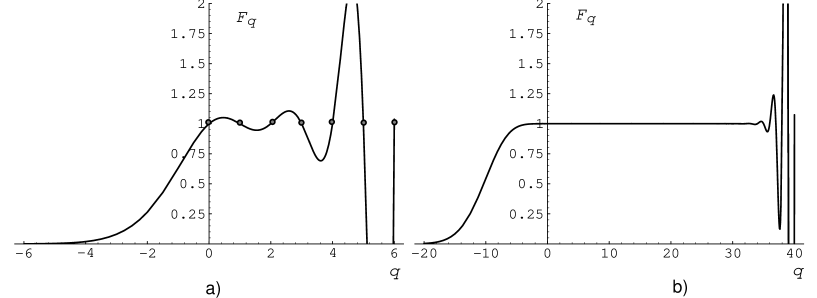
Figure 1: The Poisson GFM; a) : $n_{b}$=1, b) : $n_{b}$=10

$$F_{q} \ =\ n_{b}^{q}{\gamma(-q,n_{b})\over\Gamma(-q)}$$

$${\cal F}_{q} \ =\ F_{q}/n_{b}^{q}\ =\ \gamma^{*}(-q,n_{b})$$ (12)

where $\gamma(-q,n_{b})$ is the incomplete $\gamma$ function and $\gamma^{*}$ the analytical incomplete $\gamma$ function[17]. In any case, the value of $\gamma^{*}$ on the integer and positive (or 0) values of $q$ is 1 which is natural since one recovers here the standard factorial moments of the Poisson distribution. But one has to notice that, besides those points, the shape and behaviour of this function depends drastically on the $n_{b}$ value; This function has in fact two types of behaviour. One for $n_{b}\simeq 1$ and one for $n_{b}>>1$. This is illustrated in figure 1.

If $n_{b}\ =\ 1$ say, figure (1 a) exhibits a steeply oscillating behaviour for $q\geq 0$ and goes rapidly to 0 when $q$ is negative. This behaviour could prevent us from using those moments for small values of $n_{b}$ where one cannot wait for a faithful behaviour of the moments and where the numerical formula (7) can be very unstable. This is not a surprise if one considers that those moments are devoted to the study of rare events of low n, ie $n<<n_{b}$ For $n_{b}>>1$, say $n_{b}=10$, figure (1 b) shows that the $\gamma^{*}$ function is practically 1 in a large interval of $q$ : $-n_{b}<<q<<3n_{b}$.

¿From the point of view of the intermittency data, this indicates that the Poisson noise will be disentangled[5] from the dynamical signal only for those $q$ greater than $-n_{b}$ . As in those data the mean value of the number of particle in each bin tends rapidly to 0, one can understand that the fractional part of the moments does not gives any dynamical insight on the basic process.

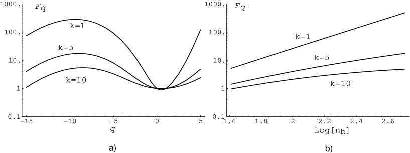
Figure 2: The GFM of the Negative Binomial Distribution. a) $q$ behaviour for $n_{b}=10$; upper curve $k=1$, intermediate one : $k=5$, lower one : $k=10$; b) $n_{b}$ behaviour at fixed $q=-5$, upper curve $k=1$, intermediate one : $k=5$, lower one : $k=4$

ii) Self similar distributions.

The best way to buid an asymptotic self-similar distribution is to construct $P_{n}$ as a compound Poisson distribution (a particular case of these distributions is the NBD distribution). At the level of the generating function, this gives:

$$G(z)\ =\ H(z-1),\ \ H(u)\ =\ \int_{0}^{\infty}\varphi(x)\exp{\big{(}ux\big{)}}dx,$$ (13)

where $\varphi$ is the usual KNO function :

$$P_{n}{\simeq}\lim_{n_{b}\to\infty}\varphi(n/n_{b})/n_{b},$$ (14)

and one gets:

$$H(u) \ =\ h(un_{b})$$

$$F_{q} \ =\ {n_{b}^{q}\over\Gamma(-q)}\int_{0}^{n_{b}}h(-u)u^{-q-1}du$$ (15)

On this integral, one can notice that if $n_{b}$ is sufficently large, ${\cal F}_{q}=F_{q}/n_{b}^{q}$ tends to a constant and we recover the KNO result provides $h(u)u^{-q}\to 0$ when $u\to\infty$. Unless this condition is fulfilled, ${\cal F}_{q}$ will depends on $n_{b}$.

If, say, $h(-u)\simeq u^{\alpha}$, when $u\to\infty$, ${\cal F}_{q}$ will be KNO for $q>>-\alpha$. When $q<-\alpha$, the integral in 2.2 will be dominated by the high u behaviour of the integrand and

$${\cal F}_{q}\ \simeq\ n_{b}^{-q+\alpha}$$ (16)

Measuring the generalised moments of the distribution provides a rather nice tool for the study of the high $u$ behaviour of the generating function.

As an exemple of this situation, we have calculated the moments of the Negative Binomial distribution :

$$h(u)\ =\ \frac{1}{(1-u/k)^{k}}$$ (17)

which gives :

$${\cal F}_{q}\ =\ \frac{{}_{2}F_{1}(k,-q,1-q,-n_{b}/k)}{n_{b}^{q}\Gamma(1-q)}$$ (18)

where ${}_{2}F_{1}$ is the hypergeometric function of the second kind[17].

The general trend of the reduced generalised moments of the distribution is given in figure (2-a) while the power-like behaviour of the moments is shown in fig (2-b).

3 QCD Generalised Moments.

3.1 QCD Double Leading-log Approximation.

The QCD evolution equation for the generating function $G(Q,z)$ of the multiplicity distribution produced by a parton of energy E disintegrating in a cone of opening $\Theta_{0}$ has been calculated since a while in the DLA approximation[10] and reads :

$$\frac{\partial G(Q,z)}{\partial\log(Q)}\ =\ G(Q,z)\int_{0}^{1}\gamma_{0}^{2}\frac{(G(xQ,z)-1)dx}{x}$$ (19)

where $Q=E\Theta_{0}$ is the hardness scale. Notice that an implicit infrared cut-off must be understood in this equation, $Qx>Q_{0}$. This cut-off tends to 0 in the weak coupling regime of the equation and will be of importance in section 3-2.

Let us first fix some notations. As in the preceding section, we define $H(Q,u)=G(Q,1-u)$, and the self similar solution (KNO) of the equation 19, $h(v)$, such as $H(Q,u)=h(n_{b}u)$. Further, for negative u, let us define ${\bf h}(y)=h(-\exp{\big{(}y\big{)}})$.

With these notations the QCD solution obeys an integro-differential equation which does not depends explicitely on the coupling constant $\gamma_{0}$, and reads (using ref.4 with some slight change of notations) :

$${d^{2}\log({\bf h})\over dy^{2}}\ =\ {\bf h}-1$$ (20)

This equation has been solved in an implicit way (for negative $u=-\exp{\big{(}y\big{)}}$[10]) :

$$y-y_{+} \ =\ \int_{\log(2)}^{X(y)}{du\over\sqrt{2(u-1+\exp{\big{(}-u\big{)}})}}$$

$$X(y) \ =\ \log(1/{\bf h}(y))\ ,\ \ \ y_{+}=-.251$$ (21)

Starting from formula (2.2), the QCD GFM for negative $q$ can be given as an $y$ integral:

$${\cal F}_{q}\ =\ \frac{1}{\Gamma(-q)}\int_{-\infty}^{\log(n_{b})}\exp{\big{(}-X(y)-qy\big{)}}dy$$ (22)

This expression is well adapted to the steepest descent technique which gives:

$$-X(y)-qy\simeq-(y-y^{*})/2\sigma^{2}-1,$$

$$y*\ =\ -q-c_{0},\ \ \sigma^{2}=1+\exp{\big{(}-q^{2}/2-1\big{)}},\ \ c_{0}=.41$$ (23)

where $c_{0}$ has been numerically computed for $y>2$. This gives asymptotically ($n_{b}\to\infty$):

$$\log({\cal F}_{q}^{qcd}) \ =\ q^{2}/2-(1-c_{0})q-1+(q-.5)\log(-q)+\log(\sigma^{2})/2,$$

$$q << -2$$ (24)

where we use the same approximation (steepest descent) for the $\Gamma$ function.

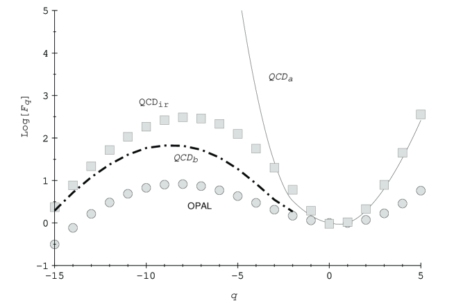
Figure 3: GFM for negative values of $q$. Continuous line : Asymptotic QCD; dotted-dashed line : finite $n_{b}$ corrections to asymptotic theory; squares : finite infrared corrections (Monte-Carlo); rounds : OPAL data (one hemisphere multiplicity)

One has now to deal with finite $n_{b}$ corrections to this formula. First we verify that the Gaussian approximation is a lower bound for ${\bf h}$, the same for the the GFM calculated with formula 22. Using formula 22 with the Gaussian approximation for ${\bf h}(y)$ as a lower bound for the finite size QCD GFM gives :

$${\cal F}_{q}(n_{b})\ =\ {\cal F}_{q}^{qcd}\Biggl{\{}{1-{\rm erf}[-(\log(n_{b})+c_{0}+q)/\sqrt{2\sigma^{2}}]\over 2}\Biggr{\}}$$ (25)

The theoretical prediction are shown in figure 3 together with the experimental data from OPAL[12]. We have taken the multiplicity data on one hemisphere in order to be as close as possible to the one parton multiplicity distribution. Notice that the prediction of the theory including finite $n_{b}$ effects has to be understood as a lower bound for the moments, specially for small values of $-q$.

3.2 Infrared effects.

Let us now turn back to formula (19). We have now to take into account the finite infrared cut-off, $Q_{0}$ of the theory.

In order to be coherent with the probabilistic interpretation of QCD DLA, the decay probability, $\Pi(x)$ of a parton of hardness $Q$ into two partons of hardness $xQ$ and $(1-x)Q$, must be normalised positive and definite . Keeping tracks only for the logarithmically divergent part of the Altarelli Parisi kernel, we have :

$$\Pi(z)=\delta(z)+\frac{\gamma_{0}^{2}}{z}\Big{|}_{+}\ =\lim_{\epsilon\to 0}\Biggl{\{}\frac{\gamma_{0}^{2}\Theta(z-\epsilon)}{z}+\delta(z)(1-\gamma_{0}^{2}\log(1/\epsilon))\Biggr{\}}$$

where $\Theta(x)$ is the Heaviside step function.

In the fixed (and finite) coupling constant case, one can observe that the probability distribution is no more positive definite in the limit $\epsilon\to 0$. As a consequance, this limit is incompatible with the building of a Monte-Carlo calculation. This is a reflection of the fact that the perturbative theory is exact only in the limit where $\gamma_{0}\to 0$, i.e. at infinite energy.

To evade this difficulty, one has to use a finite cut-off $Q_{0}$. The simplest choice is given by $\log(Q/Q_{0})\simeq 1/\gamma_{0}^{2}$ wich gives $\Pi(z)=\gamma_{0}^{2}\Theta(z-\exp{\big{(}1/\gamma_{0}^{2}\big{)}})/z$. Using this form in equation (19) gives at the level of the self-similar solution ${\bf h}$ :

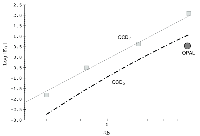
Figure 4: $n_{b}$ behaviour of ${\cal F}_{-5}$ : Continuous curve ${\cal F}_{-5}\propto n_{b}^{3}$, grey squares : QCD Monte-Carlo, dotted-dashed one QCD lower bound for finite size effects.

$$\frac{{\bf h}^{\prime}(y)}{{\bf h}(y)}\ =\ \int_{y-1/\gamma_{0}}^{y}{\bf h}(z)dz-\frac{1}{\gamma_{0}}$$ (26)

which has an asymptotic solution :

$${\bf h}(y)\ \propto\ \exp{\big{(}-\frac{y}{\gamma_{0}}\big{)}},\ \ \ y>>\frac{1}{\gamma_{0}}$$ (27)

in the limit where $y$ goes to infinity.

This exponential behaviour is different from the Gaussian solution of the QCD case (3.1). For finite $\gamma_{0}$, the infrared cut-off have changed the asymptotic behaviour of the self-similar solution of the QCD evolution equation. Notice however that one recovers the previous solution when $\gamma_{0}$ goes to 0.

As the GFM of negative order are sensitive to the high y values of the generating function, it is not astonishing that they show a different energy behaviour :

$${\cal F}_{q}\ \propto\ n_{b}^{-q-\frac{1}{\gamma_{0}}}\ =\ \big{[}\frac{E\Theta_{0}}{\mu}\big{]}^{-(1+\gamma_{0}q)}$$ (28)

This behaviour is of the NBD type (see Eq. (16)) is well reproduced by numerical (Monte-Carlo) calculations, even for low $n_{b}$.

Let us now discuss a little the QCD results. In figure 3 the Monte-Carlo results are shown to be higher than the lower bound we derived in the weak coupling limit. We verify that this does not depends on the detail of the Monte-Carlo. The infrared structure of the theory, namely the cut-off in the evolution equation, enhances the fluctuation pattern for negative values of $q$. Notice that the Monte-Carlo calculation gives the known results for positive values of $q$ which shows that the infrared cut-off has no particular effect on the standard positive moments. The OPAL data have been presented in this figure to show that the data (one hemisphere data) are substantifically lower than DLA QCD predictions in all the $q$ range. Figure 4 shows the $n_{b}$ behaviour of the GFM of order -5. It is interesting no notice that while the two QCD results are different in strength, the apparent slope of the QCD bound is close to the Monte-Carlo one and is very close to the one predicted in formula (28)$(-q-1/\gamma_{0}\simeq 3$ at LEP) .

4 Conclusions.

In this paper we have presented a comprehensive generalisation of the standard factorial moments which have been shown to be sensitive to the infrared structure of the theory. This analysis focusses on the low multiplicity events of high energy reactions such as ${\cal Z}_{0}$ decay at LEP. The QCD GFM have been calculated together with a bound on low energy corrections and have been shown to be substancially higher than the OPAL data. When one includs the natural infrared cut-off in the theory, the asymptotic picture of the GFM are modified in the negative part of its spectrum and enhances the fluctuation pattern. Our feeling is that, in contradiction to the positive $q$ case where Next to Leading-Log corrections (energy conservation effects[13]) are probably enough to explain the discrepancy of the asymptotic theory with experiments, the GFM of negative order will emphasis the non perturbative part of the theory and could provide a glance on the hadronisation part of the strong interaction theory. Further work is in progress in this direction.

Acknowledgements

It is pleasure for one of us (J.-L. M) to thanks R.Hwa and R. Peschanski for numerous and fruitful discussions on the subject, M. Le Bellac and, once more, R Peschanski for a careful reading of the manuscript.

References

- [1] Ph. Brax, J.-L. Meunier, R. Peschanski, Preprint Nice INLN 93/1-Saclay Spht/93-011, to be published in Zeit.Phys.
- [2] Y.L. Dokshitzer and I.M. Dremin Nuclear Physics B 402 (1993) 139.
- [3] W. Ochs and J. Wosiek, Phys. Lett. B289 (1992) 159, and Phys. Lett. B305 (1993) 144.
- [4] Last LEP results: DELPHI Coll., P. Abreu et al. Nucl. Phys.B386 (1992) 471; ALEPH Coll., D. Decamp et al. Z. Phys.C53 (1992) 21; See previous references (including OPAL and L3 published results, 1991) therein.
- [5] For general reviews on the subject: A. Białas Nucl. Phys. A525 (1991) 345c; R. Peschanski, Int. J. Mod. Phys.A6 (1991) 3681.
- [6] A.Bialas and R.Peschanski Nucl. Phys. B273(1991) 703 ; Nucl. Phys. B309 (1991) 897
- [7] R.Hwa Phys. Rev. D41(1991) 1456, C.B.Chiu and R.Hwa Phys. Rev. D43(1991) 100, W. Florkowski and R.Hwa Phys. Rev. D43(1991) 1548.
- [8] R.Hwa private communication and R.Hwa and J.Pan (to be published)
- [9] NA22 collaboration: M.Adamous et al., Phys.Lett.185B (1987), 200
- [10] See for example Basics of Perturbative QCD Y.L. Dokshitzer, V.A. Khoze, A.H. Mueller and S.I. Troyan (J. Tran Than Van ed., Editions Frontieres) 1991, and the list of references therein.
- [11] Z. Koba, H.B. Nielsen and P. Olesen, Nucl. Phys. B40(1972)317.
- [12] OPAL Collaboration: P.D.Acton et al Zeit.Phys.C53 (1992) 539.
- [13] Y.L. Dokshitzer Phys. Lett. B305 (1993) 295.
- [14] J.-L. Meunier and R. Peschanski, Nuclear Physics B 374 (1992) 327,
- [15] Y. Gabellini, J.-L. Meunier and R. Peschanski, Zeit. Phys. C 55 (1992) 455.
- [16] I.M. Gelfand and G.E. Chilov, Les Distributions, Dunod Paris (1965).
- [17] I.S.Gradshteyn and I.M. Ryzhik, Table of Integrals, Series and Products (Academic Press N.Y. 1980);