UAB-FT-325
CERN-TH.7141/94
HD-THEP-93-51
ISN 93–123
PM-93-44

HADRONS WITH CHARM AND BEAUTY E. Bagan^a),b),c), H.G. Dosch^b), P. Gosdzinsky^a),
S. Narison^d),e) and J.-M. Richard^f),g)
a)Grup de Física Teòrica, Dept. de Física i Institut de Física d’Altes Energies, IFAE,
Universitat Autònoma de Barcelona,

08193 Bellaterra, Spain
^b)Institut für Theoretische Physik, Universität Heidelberg,
Philosophenweg 16, 69120 Heidelberg, Germany
^c)Alexander Von-Humboldt Fellow
^d)Laboratoire de Physique Mathématique, Université de Montpellier 2,

34095 Montpellier, France
^e)CERN, Theory Division, CH-1211 Genève 23, Switzerland,

^f)Institut des Sciences Nucléaires, Université Joseph Fourier–CNRS–IN2P3
53, avenue des Martyrs, 38026 Grenoble, France
^g)European Centre for Theoretical Studies in Nuclear Physics and Related Areas (ECT)
Villa Tambosi, strada delle Tabarelle, 286, 38059 Villazzano (Trento), Italy

Abstract: By combining potential models and QCD spectral sum rules (QSSR), we discuss the spectroscopy of the $(b\bar{c})$ mesons and of the $(bcq)$, $(ccq)$ and $(bbq)$ baryons (${q}\equiv{d}$ or $s$), the decay constant and the (semi)leptonic decay modes of the $B_{c}$ meson. For the masses, the best predictions come from potential models and read: $M_{B_{c}}=(6255\pm 20)$ MeV, $M_{B^{*}_{c}}=(6330\pm 20)$ MeV, $M_{\Lambda(bcu)}=(6.93\pm 0.05)$ GeV, $M_{\Omega(bcs)}=(7.00\pm 0.05)$ GeV, $M_{\Xi^{*}(ccu)}=(3.63\pm 0.05)$ GeV and $M_{\Xi^{*}(bbu)}=(10.21\pm 0.05)$ GeV. The decay constant $f_{B_{c}}=(2.94\pm 0.21)f_{\pi}$ is well determined from QSSR and leads to: $\Gamma(B_{c}\rightarrow\nu_{\tau}\tau)=(3.0\pm 0.4)(V_{cb}/0.037)^{2}$ $\times 10^{10}$ s^-1. The uses of the vertex sum rules for the semileptonic decays of the $B_{c}$ show that the $t$-dependence of the form factors is much stronger than predicted by vector meson dominance. It also predicts the almost equal strength of about 0.30 $\times 10^{10}$ sec^-1 for the semileptonic rates $B_{c}$ into $B_{s},B^{*}_{s},\eta_{c}$ and J/$\psi$. Besides these phenomenological results, we also show explicitly how the Wilson coefficients of the $\langle\alpha_{s}G^{2}\rangle$ and $\langle G^{3}\rangle$ gluon condensates already contain the full heavy quark- ($\langle\bar{Q}Q\rangle$) and mixed- ($\langle\bar{Q}GQ\rangle$) condensate contributions in the OPE.
February, 1994

1 Introduction

With the planned high-energy machines such as the LHC, $B$-factories, the Tevatron with high luminosity, there is some hope and possibility to identify and study hadrons containing two heavy quarks [1], like double-charm baryons $(ccq)$ or hadrons with charm and beauty, namely $(b\bar{c}$) mesons and $(bcq)$ baryons. Here, and throughout this paper, $q$ denotes a light quark $u$ or $d$.

In view of this project, it is important to have safe theoretical predictions as a guide to the experimental searches of these hadrons. There are already some theoretical studies on ($b\bar{c}$) states. To our knowledge, the pioneering works on this analysis are the ones in Ref.[2] from potential models and the ones in Ref. [3] from QCD Spectral Sum Rules (QSSR) à la SVZ [4]. In this paper, we are interested in the following topics.

• Masses: so far the ground-state masses of hadrons exhibit nice regularities in flavor space, as illustrated by the Gell-Mann–Okubo mass formula, the equal-spacing rule of decuplet baryons, etc.; we would like to know the analogue of these regularity patterns in the sector of heavy quarks, and in particular interpolate $(b\bar{c})$ from $(c\bar{c})$ and $(b\bar{b})$, and extrapolate from single-charm $(cqq)$ and single-beauty $(bqq)$ baryons toward $(bcq)$ baryons with both charm and beauty.

• Decay constants: we know, in the case of the heavy–light quark systems, that the decay constants of the $D$ and $B$ mesons do not yet satisfy the 1/$\sqrt{M_{Q}}$ heavy quark scaling due to large 1/$M_{Q}$ corrections and that the prediction of the potential models based on the meson wave function fails. Then, we would like to test if the $B_{c}(\bar{b}c)$ meson decay constant can be predicted reliably from the potential models by comparing it with the one from QSSR.

• Semileptonic decay properties: we also know that QSSR vertex sum rules can predict successfully the semileptonic widths of the $D$ and $B$ mesons. Then, we pursue this application in the case of the $B_{c}$ meson.

It should be noted that the Heavy Quark Effective Theory (HQET) [6], which is successful in the heavy–light quark systems, cannot be applied straightforwardly to the $\bar{b}c$ and $\bar{b}cu$ states, unless the charm-quark mass is considered to be light, which is not a good approximation. Therefore, we combine the potential models with the QSSR approaches for estimating the masses and/or couplings of the $\bar{b}c$ and $\Lambda(bcu)$ states. The former is known to have successful predictions for the hadron masses, while its connection with QCD starts to be understood within the framework of HQET. QSSR is also known to describe successfully the hadron properties, although the accuracy of its predictions for the meson masses is limited by the systematic of the method and is less than the potential model ones. In the other cases, such as the couplings and decays, QSSR predictions are more precise and reliable.

The aim of this paper is twofold. First, we summarize the rigorous results of potential models such as mass inequalities and bounds on short-range correlations. We also present typical predictions for a “realistic” phenomenological potentials for the $\bar{b}c$ and $\Lambda(bcu)$ states. Secondly, we present improved results for the masses, couplings and form factors of the semileptonic decays from the QSSR approach.

2 Results of potential models

In this section, we first give brief reminders of general results from potential models, which can be found in reviews [7]–[11], with references to the original papers. We then summarize the rigorous and empirical results of potential models: mass inequalities, bounds on short-range correlations, typical predictions for masses and decay constants focused on the applications to the particular ($b\bar{c})$ mesons and $(bcq)$ baryons.

2.1 Constraints on the $b{\bar{c}}$ mass

Consider a purely central and flavor-independent potential. Then the binding energy depends on the flavor of the constituents only through the inverse masses $m_{1}^{-1}$ and $m_{2}^{-1}$, which enter the Hamiltonian linearly. At fixed $m_{1}$, the lowest energy is an increasing and concave function of $m_{2}^{-1}$ [12, 13]. One can for instance extrapolate the $(b\bar{c})$ energy out of the ($b\bar{s}$) and $(b\bar{q}$) energies. This gives an upper limit:

$$E(b\bar{c})\leq E(b\bar{s}){m^{-1}_{c}-m^{-1}_{q}\over m^{-1}_{s}-m^{-1}_{q}}+E(b\bar{q}){m^{-1}_{c}-m^{-1}_{s}\over m^{-1}_{q}-m^{-1}_{s}}.$$ (1)

It is independent of the $b$-quark mass, but depends upon the inverse quark masses $m^{-1}_{c}$, $m^{-1}_{s}$ and $m^{-1}_{q}$, which are not directly observable. Anyhow, (1) is not very accurate, since ($b\bar{s}$) and ($b\bar{q}$) are too close to each other to allow for a precise determination of the limiting straight line, in a plot of meson energies versus the inverse constituent masses.

In fact, better results are obtained by separating out the centre-of-mass motion, and using the inverse reduced mass $\alpha=m_{1}^{-1}+m_{2}^{-1}$, which enters the relative Hamiltonian linearly. The ground state is an increasing and concave function of $\alpha$ [12, 13]. Thus

$$(b\bar{c})\geq{(c\bar{c})+(b\bar{b})\over 2}.$$ (2)

For numerical applications of (2), one has to consider the spin-averaged masses, such as:

$$(c\bar{c})={1\over 4}\eta_{c}+{3\over 4}{\rm J}\!/\Psi$$ (3)

and its ($b\bar{b}$) analogue, with the results

$$(c\bar{c})=3.067\,\mbox{GeV},\qquad(b\bar{b})=9.448\,\mbox{GeV}$$ (4)

where experimental masses [14] are used, and an hyperfine splitting $\Upsilon-\eta_{b}=50$ MeV is assumed. This gives a lower limit

$$(b\bar{c})\geq 6.257\,\mbox{GeV}$$ (5)

for the spin averaged ($b\bar{c})$ state.

An upper limit is also obtained from the same concavity behavior in the inverse reduced mass $\alpha$:

$$(b\bar{c})\leq(b\bar{s})+(c\bar{s})-(s\bar{s}).$$ (6)

If one uses

$$(c\bar{s})=2075\,\mbox{MeV},\quad(b\bar{s})=5390\,\mbox{MeV},\quad(s\bar{s})=950\,\mbox{MeV},$$ (7)

one gets

$$(b\bar{c})\leq 6.52\,\mbox{GeV}.$$ (8)

We suspect that this bound is not very accurate, and therefore not too reliable, because it involves the strange quark. In fact one can derive an upper bound involving heavy quarks only, provided one also accounts for the excitation spectrum. The reasoning below is inspired by the work of Martin and Bertlmann [13].

From the Feynman–Hellmann theorem [12],

$${{\rm d}E\over{\rm d}\alpha}=\langle{\rm\bf p}^{2}\rangle={T(\alpha)\over\alpha},$$ (9)

where $T$ denotes the expectation value of the kinetic energy, we have

$$E(b\bar{c})=E(b\bar{b})+\int_{\alpha(b\bar{b})}^{\alpha(b\bar{c})}\alpha^{-1}T(\alpha){\rm d}\alpha.$$ (10)

and

$$E(b\bar{c})=E(c\bar{c})-\int_{\alpha(b\bar{c})}^{\alpha(c\bar{c})}\alpha^{-1}T(\alpha){\rm d}\alpha$$ (11)

We now make the mild restriction that the potential $V$ is intermediate between Coulomb and linear, and a fortiori intermediate between Coulomb and harmonic. More precisely, we assume $\Delta V\geq 0$ and $V^{\prime\prime}\leq 0$. Then

i) $T(\alpha)$ is intermediate between $\alpha^{-1}$ (Coulomb) and $\alpha^{1/3}$ (linear), i.e. $\alpha T(\alpha)$ increases with $\alpha$ while $\alpha^{-1/3}T(\alpha)$ decreases;

ii) if $\delta E=\left[E_{\rm 1P}(\alpha)-E_{\rm 1S}(\alpha)\right]/4$ denotes the orbital excitation energy, the ratio $T/\delta E$ is larger than $3/4$ (harmonic) and smaller than $4/3$ (Coulomb).

After some manipulations, we obtain

$$M(b\bar{c})\leq M(c\bar{c})+(m_{b}-m_{c})-{9\over 4}\delta E(c\bar{c})\left[1-\left({m_{b}+m_{c}\over 2m_{b}}\right)^{1/3}\right]$$

$$M(b\bar{c})\leq M(b\bar{b})-(m_{b}-m_{c})+4\delta E(b\bar{b})\left[\left({m_{b}+m_{c}\over 2m_{c}}\right)^{1/3}-1\right].$$

When they are combined, most of the dependence on the constituent masses disappears, and we obtain:

$$(b\bar{c})\leq{(c\bar{c})+(b\bar{b})\over 2}-{9\over 8}\delta E(c\bar{c})\left[1-\left({m_{b}+m_{c}\over 2m_{b}}\right)^{1/3}\right]+2\delta E(b\bar{b})\left[\left({m_{b}+m_{c}\over 2m_{c}}\right)^{1/3}-1\right]$$ (13)

After proper spin averaging of the orbital excitations [14], one finds: $\delta E(b\bar{b})\simeq\delta E(c\bar{c})\simeq 0.45\,$GeV. If one takes $m_{b}/m_{c}=3$, one obtains

$$(b\bar{c})\leq 6.43\,\mbox{GeV}.$$ (14)

Instead of working with spin-averaged masses, one could in principle write inequalities relating pseudoscalar states. If, indeed, the additional term is (including $\vec{\sigma}_{i}\cdot\vec{\sigma}_{j}=-3$) of the form

$$\delta V=-{3\over m_{1}m_{2}}V_{\rm SS},\qquad V_{\rm SS}>0,$$ (15)

then the whole Hamiltonian is a linear function of $m_{1}^{-1}$ at fixed $m_{2}^{-1}$, or a concave function of $m^{-1}$ for $m_{1}=m_{2}=m$, and one can still write some convexity inequalities. The problem is the lack of accurate experimental input for the pseudoscalar masses.

2.2 Explicit calculations of $b{\bar{c}}$ ground state

To estimate the departure from a simple additive ansatz $2(b\bar{c})=(c\bar{c})+(b\bar{b})$, one can use a logarithmic potential, which is known as a good approximation to more elaborate potentials [7]. If $V=A+B\ln(r)$, then the ground-state energy is of the form $E=A^{\prime}-B\ln(\mu)/2$. With typically $m_{b}/m_{c}=3$ and $B\sim 0.7\,$ GeV, one gets an effect

$$(b\bar{c})-{(c\bar{c})+(b\bar{b})\over 2}\simeq 0.1\,\mbox{GeV},$$ (16)

which is of course compatible with the inequalities written in the previous section.

Let us now collect some predictions of typical potential models proposed in the literature. In Ref. [15], A. Martin applied to (b$\bar{c}$) his simple power-law potential. It consists of

$$V=A+Br^{0.1}+C{\vec{\sigma}_{1}\cdot\vec{\sigma}_{2}\over m_{1}m_{2}}\delta^{(3)}({\rm\bf r}_{2}-{\rm\bf r}_{1}),$$ (17)

with $A=8.064$, $B=6.870$ and $C=1.172$, in units of powers of GeV. The quark masses are constituent masses and are $m_{s}=0.518\,$GeV, $m_{c}=1.8\,$GeV, and $m_{b}=5.174\,$GeV. The spin–spin term is treated at first order. It is adjusted to reproduce the J/$\!\Psi-\eta_{c}$ mass splitting (112 MeV [14]). He obtained

$${b\bar{c}}(0^{-})=6.25\,\mbox{GeV}\qquad{b\bar{c}}(1^{-})=6.32\,\mbox{GeV},$$ (18)

corresponding to an average of $6.30\,$GeV. These are the values also obtained by Gershtein et al. [16], who used essentially the same potential. Previously, Eichten and Feinberg, in the course of their study of spin-dependent forces [2], considered the $(b\bar{c}$) system, and got

$${b\bar{c}}(0^{-})=6.24\,\mbox{GeV}\qquad{b\bar{c}}(1^{-})=6.34\,\mbox{GeV}.$$ (19)

More recently, Eichten and Quigg [17] estimated

$${b\bar{c}}(0^{-})=6.26\,\mbox{GeV}\qquad{b\bar{c}}(1^{-})=6.33\,\mbox{GeV},$$ (20)

with a typical uncertainty of $\pm 20\,$MeV, from a survey of realistic quarkonium potentials.

One can go a little beyond the frame of this section and look at constituent models with relativistic forms of kinetic energy. They lead to the same kind of regularities as non-relativistic models, although the corresponding theorems are not always available in a fully rigorous and general form. For instance, Goodfrey and Isgur obtained

$${b\bar{c}}(0^{-})=6.27\,\mbox{GeV}\qquad{b\bar{c}}(1^{-})=6.34\,\mbox{GeV},$$ (21)

in their model [18], which tentatively describes all mesons, light or heavy.

As often in this field, there is a nice convergence of all potential models, and the uncertainty of $\pm 20\,$MeV estimated by Eichten and Quigg seems rather safe. By taking the average of different estimates and by adopting the previous uncertainty, we obtain the final estimate:

$${b\bar{c}}(0^{-})=(6255\pm 20)\,\mbox{MeV}\qquad{b\bar{c}}(1^{-})=(6330\pm 20)\,\mbox{MeV}.$$ (22)

2.3 Decay constant of mesons

For the estimate of the decay constants, let us consider the meson wave function:

$$p=\left|\Phi(0)\right|^{2}=\langle\Phi|\delta^{(3)}({\rm\bf r}_{2}-{\rm\bf r}_{1})|\Phi\rangle,$$ (23)

which governs the leptonic widths, hadronic widths, etc. It also enters the calculation of hyperfine splittings, when a simple contact term as that in Eq.  (17) is adopted.

To estimate how $p$ varies from one meson to another, let us consider first a power-law potential $V\propto r^{\beta}$. Then, from the well-known scaling laws [7, 10], one gets

$$p(\alpha)\propto\alpha^{3/(\beta+2)},$$ (24)

as a function of the inverse reduced mass $\alpha$. In particular, one expects $p\propto\alpha^{2/3}$ for a logarithmic potential, which is known to mimic the good potentials in the region of interest.

Note that one cannot object that, $p$ being the square wave function at zero separation, it is extremely sensitive to the very short-range part of the potential. In fact $p$ is given by the potential in the region where the wave function is important. This is seen on the so-called Schwinger rule [7]

$$p={1\over 4\pi\alpha}\int{\rm dr}^{(3)}|\Phi(r)|^{2}{{\rm d}V\over{\rm d}r}.$$ (25)

In short, we expect regular increases of $p$ when one goes from $c\bar{c}$ to $b\bar{b}$ via $b\bar{c}$, and presumably

$$p(b\bar{c})\leq{1\over 2}\left[p(b\bar{b})+p(c\bar{c})\right].$$ (26)

If one uses the potential model of Eq. (17), one obtains, in units of GeV³ :

$$p(c\bar{c})=0.077,\qquad p(b\bar{b})=0.350,\qquad p(b\bar{c})=0.136.$$ (27)

The absolute values are less reliable than the relative ones. Similarly, potential models usually fail in predicting the leptonic widths of the $J/\Psi$ and its radial excitations, or of the $\Upsilon$ states, but give a fair account of the ratios of leptonic widths. In terms of the wave function, the decay constant reads :

$$f_{P}=\sqrt{\frac{6p}{M_{P}}},$$ (28)

while its normalization in terms of the quark currents is:

$$(m_{c}+m_{b})<0|\bar{c}(i\gamma_{5})b|B>=\sqrt{2}M^{2}_{B_{c}}f_{B_{c}}$$

$$<0|\bar{b}\gamma^{\mu}b|\Upsilon>=\sqrt{2}M_{\Upsilon}f_{\Upsilon}\epsilon^{\mu}.$$ (29)

Then, we deduce from (27):

$$f_{B_{c}}\simeq(3.86\pm 1.31)f_{\pi}.$$ (30)

The error in this result comes from the departures of different potential-model predictions [16], [19], [17] from our value. It will be compared in section 3 with the QSSR estimates.

2.4 Inequalities on baryon masses

Let us start with a flavor- and spin-independent potential $V(\vec{r}_{1},\vec{r}_{2},\vec{r}_{3})$.

For every potential $V$, the ground-state energy is a concave function of each inverse mass $m_{i}^{-1}$. One could for instance set an upper limit on $(bcq)$ in terms of $(ccq)$ and $(csq)$, or in terms of $(csq)$ and $(cqq)$, and the corresponding quark masses. Again, it is not very useful to write inequalities that involve unobservable quark masses.

With mild restrictions on the shape of the potential, one can write convexity relations in terms of actual hadron masses [20]. For instance, there is a generalization of (2)

$$(bcq)\geq{(bbq)+(ccq)\over 2},$$ (31)

or the even more exotic looking [21]

$$(bcq)\geq{(bbb)+(ccc)+(qqq)\over 3}.$$ (32)

For numerical applications with the presently available data, one would prefer the generalization of (6)

$$(bcq)\geq(bqq)+(cqq)-(qqq).$$ (33)

This gives as a rough estimate

$$(bcq)\geq 6.9\,\mbox{GeV},$$ (34)

if one uses the rounded values $m(bqq)=5.6$, $m(cqq)=2.4$, and $m(qqq)=1.1\,$GeV.

2.5 Relations between mesons and baryons

We suppose here that there is a simple relation between the potentials governing mesons and baryons:

$$V(\vec{r}_{1},\vec{r}_{2},\vec{r}_{3})={1\over 2}\sum_{i<j}V_{q\bar{q}}(|\vec{r}_{i}-\vec{r}_{j}|).$$ (35)

There is no profound justification for this rule in QCD. We simply remark that it seems compatible with the present phenomenology. In particular, it leads to amazing inequalities among meson and baryon masses [10]. These inequalities are always satisfied when they can be checked, so one is tempted to believe that they can also hold for baryons that have not yet been discovered. For instance,

$$(bcq)\geq{(b\bar{c})+(b\bar{q})+(c\bar{q})\over 2}.$$ (36)

With the spin-averaged masses $m(B)=5.3$ and $m(D)=1.97\,$GeV, and with our previous lower bound (5) on ($b\bar{c}$), one obtains

$$(bcq)\geq 6.73\,\mbox{GeV}.$$ (37)

We suspect this to be a rather crude lower bound, and, indeed, it does not improve our previous lower bound (34). In deriving Eq. (36), one neglects the motion of the centre of mass of any quark pair in the overall rest frame of the baryon. Improvements are feasible, to better express 3-body energies in terms of 2-body energies, but the latter are no longer too easily expressed as energies of actual mesons [22, 23].

2.6 Explicit model calculations of $(bcq)$ masses

Unfortunately, there are not too many explicit computations of the masses of baryons with two heavy quarks, at least to our knowledge. The case of $(ccq)$ baryons was considered by Fleck and Richard [24]. They first use a non-relativistic potential model. Not surprisingly, the exact solution of the 3-body problem is well reproduced by a Born–Oppenheimer approximation. This opens the possibility of treating the light quark relativistically, for a fixed separation of the heavy quarks. This was done in Ref. [24], where a variant of the MIT bag model was used. It was found, however, that the results are rather sensitive to the details of the bag model. We shall not consider them further and restrict ourselves to the potential-model picture. In principle, the Born–Oppenheimer treatment could be repeated, with the gluon and light-quark degrees of freedom treated via sum rules or via a lattice simulation, at fixed QQ separation.

The results for (ccq) are obtained with a simple local and pairwise interaction

$$V_{\rm T}={1\over 2}\sum_{i<j}V,$$ (38)

where the factor $1/2$ is an arbitrary convention (though reminiscent from the discussion in Sec. 2.5, and $V$ is a variant of the power-law potential (17), adjusted to fit all ground-state baryons [25]. The parameters are $A=-8.337$, $B=6.9923$, $C=2.572$, where units are powers of GeV. As for the constituent masses, which should not be confused with the masses used in the QSSR analysis, we use $m_{\rm q}=0.300$, $m_{\rm s}=0.600$, and $m_{\rm c}=1.905\,$GeV. The latter value is 10 MeV above the c-quark mass in Refs. [25, 24], to better reproduce the experimental mass of the $\Lambda_{\rm c}$ at 2285 MeV [14]. The $\Sigma_{\rm c}-\Lambda_{\rm c}$ difference comes out right. If one takes for the b quark a mass $m_{\rm b}=5.290$, one obtains a reasonable $\Lambda_{\rm b}$ at $5.620\,$GeV, which is the central value recently reported [26].

We keep these parameters fixed to calculate the masses given in Table 1, namely the spin-averaged mass $\,\overline{\!M}$ (computed without the spin–spin term), and the lowest spin-$1/2$ state.

State	$\,\overline{\!M}$	$M_{0}$
$(ccq)$	13.70	13.63
$(ccs)$	13.80	13.72
$(bbq)$	10.24	10.21
$(bbs)$	10.30	10.27
$(bcq)$	16.99	16.93
$(bcs)$	17.07	17.00

Table 1: Masses of heavy baryons with a simple power-law potential fitted to known baryons. $\,\overline{\!M}$ is the spin averaged mass, and $M_{0}$ that of the lowest state, with spin-$1/2$. Units are GeV.

A remark concerning the spin structure: the lowest $(ccq)$ baryon has spin $S=1/2$, with the $(cc)$ pair in a spin $s=1$ state, as dictated by the statistics. For $(bcq)$, we have a mixing of $s=0$ and $s=1$, with the latter dominating, to leave maximal strength for $(qc)$ and $(qb)$ pairs (for total spin $S=1/2$, the cumulated $\sum_{i<j}\vec{\sigma}_{i}\cdot\vec{\sigma}_{j}$ is fixed at the value $-3$, independent of the internal spin structure).

We estimate the theoretical uncertainty around $\pm 20$ MeV in the extrapolation. The main additional uncertainty comes from the mass of $\Lambda_{\rm b}$. Altogether we obtain

$$\Lambda(bcq)=6.93\pm 0.05\,\mbox{GeV}\quad\Omega(bcs)=7.00\pm 0.05\,\mbox{GeV}.$$ (39)

We can also deduce from Table 1, the masses of the ${\Xi^{*}_{c}}(ccu)$ and ${\Xi^{*}_{b}}(bbu)$ with the same degree of accuracy of 50 meV. The result for $\Lambda(bcq)$ agrees quite well with the improved QSSR estimate which will be discussed in the next section. The ones for $\Xi^{*}_{c,b}$ agree with the QSSR estimates in [27] which will also be reminded section 3.

2.7 Short-range correlations in baryons

The quantity $p$ defined in Eq. (23) for mesons is generalized as

$$p_{ij}=\langle\Phi|\delta^{(3)}({\rm\bf r}_{j}-{\rm\bf r}_{i})|\Phi\rangle.$$ (40)

We are not aware of too many results on the coefficients $p_{ij}$. The Schwinger rule (25) has been generalized [28], but the sum rule now involves centrifugal barriers (in an $s$-wave baryon, the pairs are not strictly in a state of orbital momentum $\ell=0$, except in the harmonic-oscillator case), and angular correlations like $\hat{\rm r}_{ij}\cdot\hat{\rm r}_{ik}$. The available results concern symmetric and nearly symmetric cases. References can be found in [10].

For the very asymmetric cases we are dealing with, we simply read the values of the $p_{ij}$ from the wave function, which is computed with our simple power-law potential, using the method of hyperspherical harmonics [10]. The results are shown in Table 2.

State	$p_{12}$	$p_{23}$	$p_{31}$	$10^{3}p_{123}$
$(ccq)$	0.039	0.009	0.009	0.36
$(ccs)$	0.042	0.019	0.019	0.36
$(bbq)$	0.152	0.012	0.012	4.08
$(bbs)$	0.162	0.028	0.028	4.09
$(bcq)$	0.065	0.010	0.011	0.90
$(bcs)$	0.071	0.021	0.025	0.90

Table 2: Short-range correlation coefficients $p_{ij}$ calculated with our simple power-law potential. Units are GeV³ for the 2-body terms $p_{ij}$, and GeV⁶ for $p_{123}$.

Some remarks are in order:

i) The correlation between two quarks depends on the third one [29].

ii) There are more correlations between $b$ and $\bar{c}$ in a ($b\bar{c}$) meson than between $b$ and $c$ in $(bcq)$ or $(bcs)$.

The coupling constants $|Z|^{2}$ that are usually quoted (see, e.g. Ref. [42]–[44], [27]) have more to do with the probability $p_{123}$ of finding the three quarks at the same place in the non-relativistic wave function. Some values of $p_{123}$ are shown in Table 2. The normalization requires some technicalities. We define

$$p_{123}=\langle\Phi|\delta^{(3)}({\rm\bf x})\delta^{(3)}({\rm\bf y})|\Phi\rangle,$$ (41)

where the Jacobi variables are introduced as

$${\rm\bf x}={\rm\bf r}_{2}-{\rm\bf r}_{1}$$

$${\rm\bf y}=\left[{\rm\bf r}_{3}-{m_{1}{\rm\bf r}_{1}+m_{2}{\rm\bf r}_{2}\over m_{1}+m_{2}}\right](m_{1}+m_{2})\sqrt{{m_{3}\over m_{1}m_{2}(m_{1}+m_{2}+m_{3})}}$$ (42)

(the coefficient of ${\rm\bf y}$ is such that the kinetic energy operator is proportional to ${\rm d}^{2}/{\rm d}{\rm\bf x}^{2}+{\rm d}^{2}/{\rm d}{\rm\bf y}^{2}$), and the labeling is such that 1 and 2 are the heavy quarks, and 3 the light one.

3 The $B_{c}$, $\Lambda(bcu)$ , ${\Xi^{*}_{c}}(ccu)$ and ${\Xi^{*}_{b}}(bbu)$ masses and couplings from QSSR

We have studied in the previous section the properties of the $B_{c}$ meson, $\Lambda(bcq)$, $\Xi^{*}_{c}$ and $\Xi^{*}_{b}$ baryons using potential models. In the following, we shall study their properties using the QSSR approach.

3.1 The $B_{c}$-meson correlator

We shall be concerned with the two-point correlator:

$$\psi_{5}(q^{2})=i\int d^{4}x\,\mathrm{e}^{iq\cdot x}\langle 0|{\bf T}J_{5}(x){J^{\dagger}}_{5}(0)|0\rangle$$ (43)

associated to the pseudoscalar current:

$$J_{5}(x)=(m_{c}+m_{b}):\overline{b}(i\gamma_{5})c:$$ (44)

The spectral function $\Im\mathrm{m}\psi_{5}(t)$ can be evaluated in QCD for $t\gg\Lambda^{2}$. Its perturbative part is known to two loops in terms of the pole quark masses [30]. It reads:

$$\mbox{Im}\psi_{5}^{\rm pert}(t) = {3(m_{b}+m_{c})^{2}\over 8\pi t}\bar{q}{}^{4}v\Bigg{\{}1+{4\alpha_{s}\over 3\pi}\Bigg{\{}{3\over 8}(7-v^{2})$$

$$+ \sum_{i=b,c}\Big{[}(v+v^{-1})\left(L_{2}(\alpha_{1}\alpha_{2})-L_{2}(-\alpha_{i})-\log\alpha_{1}\;\log\beta_{i}\right)$$

$$+ A_{i}\log\alpha_{i}+B_{i}\log\beta_{i}\Big{]}\Bigg{\}}+O(\alpha_{s}^{2})\Bigg{\}}$$

where

$$L_{2}(x)=-\int_{0}^{x}{dy\over y}\log(1-y)$$ (46)

and

$$A_{i} = {3\over 4}{3m_{i}+m_{j}\over m_{i}+m_{j}}-{19+2v^{2}+3v^{4}\over 32v}-{m_{i}(m_{i}-m_{j})\over\bar{q}{}^{2}v(1+v)}\left(1+v+{2v\over 1+\alpha_{i}}\right);$$

$$B_{i} = 2+2{m_{i}^{2}-m_{j}^{2}\over\bar{q}{}^{2}v};$$ (47)

$$\alpha_{i} = {m_{i}\over m_{j}}{1-v\over 1+v};\qquad\beta_{i}=\sqrt{1+\alpha_{i}}\;{(1+v)^{2}\over 4v}$$

$$\bar{q}{}^{2} = t-(m_{b}-m_{c})^{2};\qquad v=\sqrt{1-4{m_{b}m_{c}\over\bar{q}{}^{2}}}$$

The non-perturbative pieces of Im $\psi_{5}(t)$ can be introduced using an OPE à la SVZ [4]. We shall consider the contributions of operators up to dimension six. Following the usual procedure in Ref. [31], we obtain the Wilson coefficients of the $\langle G^{2}\rangle$ and $\langle G^{3}\rangle$ gluon condensates. The diagrams involved are shown in Fig. 1.

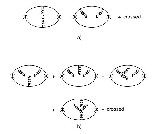
Figure 1: a) Diagrams contributing to the gluon condensate coefficient ${\rm Im}\,C_{G^{2}}$. b) Diagrams contributing to the three-gluon condensate coefficient ${\rm Im}\,C_{G^{3}}$.

Our results are:

$$\mbox{Im}\,C_{G^{2}} = -{\alpha_{s}m_{b}m_{c}\,t\over 2[t-(m_{b}-m_{c})^{2}]^{3/2}}$$ (48)

$$\times \left(t-m_{b}^{2}-m_{b}m_{c}-m_{c}^{2}\right){\theta[t-(m_{b}+m_{c})^{2}]\over[t-(m_{b}+m_{c})^{2}]^{5/2}}+\cdots$$

$$\mbox{Im}\,C_{G^{3}} = {\alpha_{s}m_{b}m_{c}\;t\over 6\;[t-(m_{b}-m_{c})^{2}]^{7/2}}\left\{3t^{4}-2(3m_{b}^{2}+2m_{b}m_{c}+3m_{c}^{2})t^{3}\right.$$ (49)

$$+ (5m_{b}^{3}m_{c}+18m_{b}^{2}m_{c}^{2}+5m_{b}m_{c}^{3})\;t^{2}$$

$$+ 2(3m_{b}^{6}+m_{b}^{5}m_{c}-6m_{b}^{4}m_{c}^{2}-6m_{b}^{3}m_{c}^{3}-6m_{b}^{2}m_{c}^{4}+m_{b}m_{c}^{5}+3m_{c}^{6})\;t$$

$$- \left.3(m_{b}^{8}+m_{b}^{7}m_{c}-m_{b}^{5}m_{c}^{3}-2m_{b}^{4}m_{c}^{4}-m_{b}^{3}m_{c}^{5}+m_{b}m_{c}^{7}+m_{c}^{8})\right\}$$

$$\times {\theta[t-(m_{b}+m_{c})^{2}]\over[t-(m_{b}+m_{c})^{2}]^{9/2}}+\cdots$$

The dots in (48) and (49) stand for terms proportional to $\delta(t-(m_{b}+m_{c})^{2})$ and derivatives. They should be there to compensate for the singular behavior (at threshold) of $\Im\mathrm{m}C_{G^{2}}$ and $\Im\mathrm{m}C_{G^{3}}$ in a dispersion relation such as (111) in the appendix. One can circumvent the problem of computing these terms by using the method explained in the appendix. Our result for $C_{G^{2}}$ (see (6) in the appendix) agrees with previous ones [5], while the one for $C_{G^{3}}$ is new. In the equal-mass case, it agrees with the result in Refs. [35, 36].

It should be emphasized that (48) and (49) already contain the contributions of the $\langle\overline{c}c\rangle$ and $\langle\overline{c}Gc\rangle$ condensates through the heavy-quark expansion (see (52) and (53) below). In order to prove this result, let us compute $C_{G^{2}}$ and $C_{G^{3}}$ (obtained as in the appendix) for small values of $m_{c}$, retaining only the singular pieces as $m_{c}\to 0$:

$$C_{G^{2}}\!\!\!\! = \!\!\!\!-{\alpha_{s}m_{b}\over 12\pi(q^{2}-m_{b}^{2})m_{c}}-{\alpha_{s}m_{b}\,q^{2}\over 4\pi(q^{2}-m_{b}^{2})^{3}}\,m_{c}\log m_{c}^{2}+\cdots$$ (50)

$$C_{G^{3}}\!\!\!\! = \!\!\!\!-{\alpha_{s}m_{b}\over 360\pi(q^{2}\!\!-\!m_{b}^{2})m_{c}^{3}}+{\alpha_{s}(q^{2}-2m_{b}^{2})\over 720\pi(q^{2}\!\!-\!m_{b}^{2})^{2}m_{c}^{2}}+{\alpha_{s}m_{b}(15q^{2}\!\!-\!m_{b}^{2})\over 360\pi(q^{2}\!\!-\!m_{b}^{2})^{3}m_{c}}\!+\!\cdots$$ (51)

We now show that the terms of $C_{G^{2}}$ and $C_{G^{3}}$ in (50) and (51) appear because of the heavy-quark expansion, namely:

$$\langle\overline{c}c\rangle = -{1\over 12m_{c}}{\alpha_{s}\over\pi}\langle G^{2}\rangle-{1\over 360m_{c}^{3}}{\alpha_{s}\over\pi}\langle G^{3}\rangle+\cdots$$ (52)

$$\langle\overline{c}Gc\rangle = {m_{c}\over 2}\log m_{c}^{2}\;{\alpha_{s}\over\pi}\langle G^{2}\rangle-{1\over 12m_{c}}{\alpha_{s}\over\pi}\langle G^{3}\rangle+\cdots$$ (53)

To see this, let us give the quark and mixed condensate coefficients for the pseudoscalar current (which can be found in [32], appendix A). In our notation:

$$C_{\bar{c}c} = {m_{b}\over q^{2}-m_{b}^{2}}+{2m_{b}^{2}-q^{2}\over 2(q^{2}-m_{b}^{2})^{2}}m_{c}+{m_{b}^{3}\over(q^{2}-m_{b}^{2})^{3}}m_{c}^{2}+\cdots$$ (54)

$$C_{\bar{c}Gc} = -{m_{b}q^{2}\over 2(q^{2}-m_{b}^{2})^{3}}+\cdots$$ (55)

Note that multiplying (54) and (55) by (52) and (53), respectively, and adding the two contributions, one obtains (50) and (51). This clearly shows that our results for $C_{G^{2}}$ and $C_{G^{3}}$ already contain the parametrization of the quark and mixed condensates in terms of purely gluonic operators, as already shown in the literature (see for instance [33]).

3.2 The $B_{c}$-meson coupling

The $B_{c}$-meson is introduced via its coupling $F_{B_{c}}$ as:

$$\langle 0|J_{5}|B_{c}\rangle=\sqrt{2}F_{B_{c}}M_{B_{c}}^{2},$$ (56)

while the contribution of higher radial excited states are averaged from the QCD continuum above the threshold $t_{c}$. After transferring the continuum effect into the QCD side of the spectral function, the coupling $F_{B_{c}}$ can be estimated from the finite energy sum rule moments:

$$\mathcal{M}^{(n)}=\int_{(m_{b}+m_{c})^{2}}^{t_{c}}{dt\over t^{n+2}}{1\over\pi}\mbox{Im}\,\psi_{5}(t)$$ (57)

or the Laplace sum rule:

$$\mathcal{L}=\int_{(m_{b}+m_{c})^{2}}^{t_{c}}dt\;\mathrm{e}^{-t\tau}{1\over\pi}\mbox{Im}\,\psi_{5}(t),$$ (58)

while the $B_{c}$-mass squared can be obtained from the ratios:

$${\mathcal{R}} = {\mathcal{M}^{(n)}\over\mathcal{M}^{(n)}+1}$$ (59)

$${\mathcal{R}}_{\mathcal{L}} = -{1\over\mathcal{L}}{d\mathcal{L}\over d\tau}.$$ (60)

Here $n$, $\tau$ and $t_{c}$ are in general free external parameters in the analysis, so that the optimal results should be insensitive to their values (stability criteria). The first QSSR estimates of the $B_{c}$-meson mass and couplings [3] are:

$$M_{B_{c}}=(6.5\pm 0.4)\,\mbox{GeV}\ \ ,\ \ f_{B_{c}}=(3.7\pm 0.5)f_{\pi},$$ (61)

where the uncertainties due to the mass and to the subtraction scale (This scale does not appear in the present paper, as can be inferred from Refs. [33, 36]. Thus, the parametrization given by Ref. [37] and used in the previous paper is not correct.) entering in the mixed condensate imply a large error in the estimate of the coupling $F_{B_{c}}$. For improving this result, we shall use the potential-model predictions in eq. (22) and estimate $F_{B_{c}}$ from the sum rules in (57) and (58). We show the results of the analysis in Fig. 2.

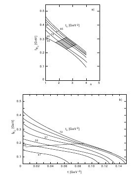
Figure 2: a)$n$-dependence of the decay constant $f_{B_{c}}$ for different values of the continuum threshold $t_{c}$. b) $\tau$-dependence of the decay constant $f_{B_{c}}$ for different values of the continuum threshold $t_{c}$.

As one can see in this figure, the stability corresponds to the inflexion point so that its localization is less precise than for the case of the minimum (these inflexion points are indicated by the shaded region in Fig. 2a and by the line in Fig. 2b). We assume that this will imply a $10\%$ error. Taking the largest range of $t_{c}$-values from the onset of the $n$- or $\tau$-stability region ($t_{c}\simeq 50$ GeV²) until the onset of the $t_{c}$-stability region ($t_{c}\simeq 67$ GeV²) and by taking the average of these two extreme values, we obtain:

$$F_{B_{c}}|_{Laplace}\simeq(2.95\pm 0.27)f_{\pi}$$ (62)

and:

$$F_{B_{c}}|_{Moments}\simeq(2.84\pm 0.38)f_{\pi}.$$ (63)

We have used the values [5]:

$$\langle\alpha_{s}G^{2}\rangle = (0.06\pm 0.02)\mbox{GeV}^{4}$$

$$m_{b}(p^{2}=m_{b}^{2}) = (4.60\pm 0.05)\mbox{GeV}$$ (64)

$$m_{c}(p^{2}=m_{c}^{2}) = (1.47\pm 0.05)\mbox{GeV}$$

$$\langle g^{3}G^{3}\rangle = (1.2\mbox{GeV}^{2})\times\langle\alpha_{s}G^{2}\rangle,$$

from a global QSSR analysis of different hadronic channels. The $\langle G^{3}\rangle$ value is based on a rough estimate within the dilute gas instanton model [37].

The main errors in $F_{B_{c}}$ come from the localization of the inflexion point. One should notice that, at the inflexion point, the $\alpha_{s}$-correction does not exceed $10\%$ of the leading-order term for the two-point correlator. Contrary to the other QSSR analysis, the non-perturbative terms are negligible and do not play a role in the optimization procedure so that the optimal region is not well indicated. However, the smallness of the non-perturbative terms indicates that the OPE converges quite well at the optimization scale. This value of $F_{B_{c}}$ agrees and improves (from the inclusion of the $G^{3}$-term) the pioneer results in Refs. [3, 5, 34]. Taking the average of the two QSSR values, we deduce:

$$F_{B_{c}}|_{average}\simeq(2.94\pm 0.22)f_{\pi}.$$ (65)

It is important to notice that the continuum energy $E_{c}$ defined as:

$$t_{c}\equiv(m_{b}+m_{c}+E_{c})^{2}$$ (66)

is:

$$E_{c}\simeq(1.0\sim 2.1)\,\mbox{GeV},$$ (67)

in good agreement with what we know in the optimization of the sum rule for the heavy–light quark systems [38, 39]. The result $F_{B_{c}}\simeq 1.22f_{\pi}$ obtained in Ref.[40] is too low, which should be due to numerical errors as far as the result obtained from the moments in that paper is concerned. The other possible source of uncertainties, in this paper, is the value of the continuum threshold used in the analysis, which is too low. The result of Ref. [41] is more similar to ours, but the procedure used by the authors to derive it is very doubtful. Indeed, we do not see any physical reasons to move the $t_{c}$ values inside a small range from 47 to 50 GeV², which is outside the stability region in (65). The $M^{2}$ sum rule variable stability shown in their paper and translated in terms of the $\tau\equiv 1/M^{2}$ used in our paper ranges between 0.04 and 0.13 GeV^-2, in agreement with ours, but appears too small compared with other channels studied until now within QSSR. This is because the non-perturbative terms do not play any essential role in the analysis.

Our results agree with the one indicated by the potential models in (30). If we tentatively average the result in (63) with the previous potential one in (30), we can deduce:

$$F_{B_{c}}|_{average}\simeq(2.94\pm 0.21)f_{\pi},$$ (68)

which we consider to be our final estimate.

3.3 The $\Lambda(bcu)$ correlator

Let us consider the baryonic current:

$$J=r_{1}\,\left(u^{t}{\cal C}\gamma^{5}c\right)b+r_{2}\,\left(u^{t}{\cal C}c\right)\gamma^{5}b+r_{3}\,\left(u^{t}{\cal C}\gamma^{5}\gamma^{\mu}c\right)\gamma_{\mu}b$$ (69)

which has the quantum numbers of the $\Lambda(bcu)$; $r_{1}$, $r_{2}$ and $r_{3}$ are arbitrary mixing parameters where, in terms of the $b$ parameter used in Ref. [43]:

$$r_{1}=(5+b)/\;2\sqrt{6};\quad r_{2}=(1+5b)/\;2\sqrt{6};\quad r_{3}=(1-b)/\;2\sqrt{6}.$$ (70)

The choice of operators in Ref. [27] is recovered in the particular case where:

$$r_{1}=1;\quad r_{2}=k;\quad r_{3}=0.$$ (71)

The associated two-point correlator is:

$$i\int d^{4}x\;\mathrm{e}^{ip\cdot x}\langle 0|{\bf T}J(x)\overline{J}(0)|0\rangle=\not{p}F_{1}+F_{2}.$$ (72)

The QCD expressions of the form factors $F_{1}$ and $F_{2}$ can be parametrized as:

$$F_{i}=F_{i}^{{\rm Pert}}+F_{i}^{G}+F_{i}^{{\rm Mix}},$$ (73)

where:

$$\mbox{Im}\;F_{2}^{\rm Pert}(t) = {1\over 128\pi^{3}t}\left\{(2r_{3}^{2}+r_{2}^{2}-r_{1}^{2})\,m_{b}\,\left\{6\left[m_{b}^{2}t^{2}+(m_{b}^{4}-2m_{b}^{2}m_{c}^{2}-m_{c}^{4})t\right.\right.\right.$$ (74)

$$+ 2\left.m_{b}^{2}m_{c}^{4}\right]\,{\cal L}_{1}-6t\left[m_{b}^{2}\,t+(m_{b}^{2}-m_{c}^{2})^{2}\right]\,{\cal L}_{2}$$

$$- \left.\left[t^{2}+5(2m_{b}^{2}-m_{c}^{2})t+m_{b}^{4}-5m_{b}^{2}m_{c}^{2}-2m_{c}^{4}\right]\;\lambda_{bc}^{1/2}\right\}$$

$$- 2r_{1}r_{3}\,m_{c}\left\{6\left[m_{c}^{2}t^{2}+(m_{c}^{4}-2m_{c}^{2}m_{b}^{2}-m_{b}^{4})t+2m_{c}^{2}m_{b}^{4}\right]{\cal L}_{1}\right.$$

$$+ 6t\left[m_{c}^{2}\,t+(m_{c}^{2}-m_{b}^{2})^{2}\right]{\cal L}_{2}$$

$$- \left.\left.\left[t^{2}+5(2m_{c}^{2}-m_{b}^{2})t+m_{c}^{4}-5m_{c}^{2}m_{b}^{2}-2m_{b}^{4}\right]\;\lambda_{cb}\right\}\right\}$$

$$\mbox{Im}\;F_{2}^{\psi}(t) = {\langle\overline{\psi}\psi\rangle\over 8\pi t}\lambda_{bc}^{1/2}\left\{-(r_{1}^{2}+r_{2}^{2}+4r_{3}^{2})m_{b}m_{c}+r_{1}r_{3}\;(m_{b}^{2}+m_{c}^{2}-t)\right\}$$ (75)

$$\mbox{Im}\;F_{2}^{G}(t) = {\langle\alpha_{s}\,G^{2}\rangle\over 384\pi^{2}t}\left\{\left[2{r_{3}^{2}\over m_{b}}\left(-2t+7m_{b}^{2}+2m_{c}^{2}\right)\right.\right.$$ (76)

$$+ {r_{1}^{2}-r_{2}^{2}\over m_{b}}\left(2t+5m_{b}^{2}-2m_{c}^{2}\right)+2{r_{1}r_{3}\over m_{c}}\left(2t-2m_{b}^{2}-m_{c}^{2}\right)$$

$$+ \left.12r_{2}r_{3}\,m_{c}\phantom{{r_{3}^{2}\over m_{b}}}\kern-14.22636pt\right]\lambda_{bc}^{1/2}$$

$$+ 6\left[(r_{2}^{2}-r_{1}^{2})\,m_{b}\,t+2r_{3}^{2}m_{b}m_{c}^{2}-r_{1}r_{3}m_{c}t-r_{2}r_{3}m_{c}\,(t-2m_{b}^{2})\right]{\cal L}_{1}$$

$$- \left.6t\left[(r_{2}^{2}-r_{1}^{2})m_{b}+(r_{1}+r_{2})r_{3}m_{c}\right]\,{\cal L}_{2}\phantom{{r_{3}^{2}\over m_{b}}}\kern-14.22636pt\right\}$$

$$\mbox{Im}\;F_{2}^{\rm Mix}(t) = {M_{0}^{2}\langle\overline{\psi}\psi\rangle\over 64\pi t\,\lambda_{bc}^{3/2}}\left\{2(r_{1}^{2}+r_{2}^{2})\,m_{b}m_{c}\left[-t^{3}+t^{2}(m_{b}^{2}+3m_{c}^{2})\right.\right.$$ (77)

$$+ \left.t(m_{b}^{2}+m_{c}^{2})(m_{b}^{2}-3m_{c}^{2})-(m_{b}^{2}-m_{c}^{2})^{3}\right]$$

$$+ 4r_{3}^{2}m_{b}m_{c}\left[-t^{3}+t^{2}(3m_{b}^{2}+m_{c}^{2})\right.$$

$$+ \left.t(-3m_{b}^{4}-6m_{b}^{2}m_{c}^{2}+m_{c}^{4})+(m_{b}^{2}-m_{c}^{2})^{3}\right]$$

$$+ 2r_{1}r_{3}\left[t^{4}+t^{3}(-3m_{b}^{2}-2m_{c}^{2})+3t^{2}m_{b}^{2}(m_{b}^{2}-m_{c}^{2})\right.$$

$$+ \left.t(-m_{b}^{6}+4m_{b}^{4}m_{c}^{2}+3m_{b}^{2}m_{c}^{4}+2m_{c}^{6})+m_{c}^{2}(m_{b}^{2}-m_{c}^{2})^{3}\right]$$

$$+ 2r_{2}r_{3}\left[t^{4}+t^{3}(-4m_{b}^{2}-3m_{c}^{2})+3t^{2}(2m_{b}^{4}+m_{b}^{2}m_{c}^{2}+m_{c}^{4})\right.$$

$$- \left.\left.t(m_{b}^{2}-m_{c}^{2})(4m_{b}^{4}+m_{b}^{2}m_{c}^{2}-m_{c}^{4})+m_{b}^{2}(m_{b}^{2}-m_{c}^{2})^{3}\right]\right\}$$

$$\mbox{Im}\;F_{1}^{\rm Pert}(t) = {1\over 512\pi^{3}t^{2}}\left\{(r_{1}^{2}+r_{2}^{2}+4r_{3}^{2})\left\{12\left[t^{2}(m_{b}^{4}+m_{c}^{4})-2m_{b}^{4}m_{c}^{4}\right]\,{\cal L}_{1}\right.\right.$$ (78)

$$- 12t^{2}(m_{b}^{4}-m_{c}^{4})\,{\cal L}_{2}$$

$$+ \left[t^{3}-7t^{2}(m_{b}^{2}+m_{c}^{2})+t(-7m_{b}^{4}+12m_{b}^{2}m_{c}^{2}-7m_{c}^{4})\right.$$

$$+ \left.\left.m_{b}^{6}-7m_{b}^{4}m_{c}^{2}-7m_{b}^{2}m_{c}^{4}+m_{c}^{6}\right]\;\lambda_{bc}^{1/2}\right\}$$

$$- 4r_{1}r_{3}\,m_{b}m_{c}\left\{12\left[t^{2}(m_{b}^{2}+m_{c}^{2})-4tm_{b}^{2}m_{c}^{2}+2m_{b}^{2}m_{c}^{2}(m_{b}^{2}+m_{c}^{2})\right]{\cal L}_{1}\right.$$

$$- 12t^{2}(m_{b}^{2}-m_{c}^{2})\,{\cal L}_{2}$$

$$- \left.\left.2\left[2t^{2}+5t(m_{b}^{2}+m_{c}^{2})-m_{b}^{4}-10m_{b}^{2}m_{c}^{2}-m_{c}^{4}\right]\;\lambda_{cb}\right\}\right\}$$

$$\mbox{Im}\;F_{1}^{\psi}(t) = {\langle\overline{\psi}\psi\rangle\over 16\pi t^{2}}\lambda_{bc}^{1/2}\left\{(2r_{3}^{2}+r_{2}^{2}-r_{1}^{2})\,m_{c}(t+m_{b}^{2}-m_{c}^{2})\right.$$ (79)

$$+ \left.2r_{1}r_{3}\,m_{b}(m_{b}^{2}-m_{c}^{2}-t)\right\}$$

$$\mbox{Im}\;F_{1}^{G}(t) = {\langle\alpha_{s}\,G^{2}\rangle\over 768\pi^{2}t^{2}}\left\{\left[-4r_{3}^{2}\left(t+3m_{b}^{2}\right)-(r_{2}^{2}+r_{1}^{2})\left(t-3m_{b}^{2}+3m_{c}^{2}\right)\right.\right.$$ (80)

$$+ 4{r_{1}r_{3}\over m_{b}m_{c}}\left(2t\,(m_{b}^{2}+m_{c}^{2})-2m_{b}^{4}-11m_{b}^{2}m_{c}^{2}-2m_{c}^{4}\right)$$

$$- \left.36r_{2}r_{3}\,m_{b}m_{c}\right]\lambda_{bc}^{1/2}$$

$$+ 12m_{b}m_{c}\left[-2r_{3}^{2}\,m_{b}m_{c}+2r_{1}r_{3}\left(t-2m_{b}^{2}-3m_{c}^{2}\right)\right.$$

$$+ \left.\left.2r_{2}r_{3}\left(t-m_{b}^{2}-2m_{c}^{2}\right)\right]{\cal L}_{1}\right\}$$

$$\mbox{Im}\;F_{1}^{\rm Mix}(t) = {M_{0}^{2}\langle\overline{\psi}\psi\rangle\over 64\pi t^{2}\,\lambda_{bc}^{3/2}}\left\{2(r_{1}^{2}-r_{2}^{2})\,m_{c}\left[-t^{4}+t^{3}(2m_{b}^{2}+5m_{c}^{2})\right.\right.$$ (81)

$$- t^{2}(2m_{b}^{4}+3m_{b}^{2}m_{c}^{2}+9m_{c}^{4})+t(m_{b}^{2}-m_{c}^{2})(2m_{b}^{4}-m_{b}^{2}m_{c}^{2}-7m_{c}^{4})$$

$$- \left.(m_{b}^{2}-m_{c}^{2})^{3}(m_{b}^{2}-2m_{c}^{2})\right]$$

$$+ 2r_{3}^{2}m_{c}\left[t^{3}(m_{b}^{2}-m_{c}^{2})+t^{2}(-3m_{b}^{4}+4m_{b}^{2}m_{c}^{2}+3m_{c}^{4})\right.$$

$$+ \left.3t(m_{b}^{2}-m_{c}^{2})(m_{b}^{2}+m_{c}^{2})^{2}-(m_{b}^{2}-m_{c}^{2})^{3}(m_{b}^{2}+m_{c}^{2})\right]$$

$$+ 2r_{1}r_{3}\,m_{b}\left[-t^{4}+t^{3}(5m_{b}^{2}+m_{c}^{2})+t^{2}(-9m_{b}^{4}-4m_{b}^{2}m_{c}^{2}+m_{c}^{4})\right.$$

$$+ \left.t(m_{b}^{2}-m_{c}^{2})(7m_{b}^{4}+4m_{b}^{2}m_{c}^{2}+m_{c}^{4})-2m_{b}^{2}(m_{b}^{2}-m_{c}^{2})^{3}\right]$$

$$+ 2r_{2}r_{3}m_{b}\left[-t^{4}+2t^{3}(2m_{b}^{2}+m_{c}^{2})-2t^{2}(3m_{b}^{4}+m_{c}^{4})\right.$$

$$+ \left.\left.2t(2m_{b}^{6}-3m_{b}^{4}m_{c}^{2}+m_{c}^{6})-(m_{b}^{2}-m_{c}^{2})^{4}\right]\right\},$$

with:

$$\begin{array}[]{lcllcl}{\cal L}_{1}(t)\!\!\!&=&\!\!\!\displaystyle{{1\over 2}\log{1+v\over 1-v};}&v\!\!\!&=&\!\!\!\displaystyle{\sqrt{1-{4m_{b}^{2}m_{c}^{2}\over(t-m_{b}^{2}-m_{c}^{2})^{2}}}}\\ \lambda_{bc}^{1/2}\!\!\!&=&\!\!\!(t-m_{b}^{2}-m_{c}^{2})\,v;&{\cal L}_{2}\!\!\!&=&\!\!\!\displaystyle{\log{(m_{b}^{2}+m_{c}^{2})t+(m_{b}^{2}-m_{c}^{2})(\lambda_{bc}^{1/2}-m_{b}^{2}+m_{c}^{2})\over 2m_{b}m_{c}\,t}}.\\ &=&\!\!\!\lambda^{1/2}(m_{b}^{2},m_{c}^{2},t)&&&\end{array}$$ (82)

The QCD expressions in Ref. [27] are recovered for the values of $r_{i}$ in (71). Those in Ref. [43] are obtained by taking the value of $r_{i}$ in (70), letting $m_{c}\to 0$. This is a non-trivial check that we now discuss in some detail. For the perturbative part one has to take into account that:

$${\cal L}_{1} {\buildrel m_{c}\to 0\over{\longrightarrow}} {1\over 2}\log{t\over m_{c}^{2}}+{1\over 2}\log{(t-m_{b}^{2})^{2}\over m_{b}^{2}t}+\cdots$$

$${\cal L}_{2} {\buildrel m_{c}\to 0\over{\longrightarrow}} {1\over 2}\log{t\over m_{c}^{2}}+{1\over 2}\log{m_{b}^{2}(t-m_{b}^{2})^{2}\over t^{3}}+\cdots$$ (83)

$$\lambda_{bc}^{1/2} {\buildrel m_{c}\to 0\over{\longrightarrow}} t-m_{b}^{2}+\cdots$$

For the quark condensate, one must recall that when $m_{c}\to 0$ the $c$-quark must be allowed to condense. The easiest way to find this new $c$-quark condensate contribution consists in isolating the $1/m_{c}$ poles in the gluon condensate coefficients and using the first term of the heavy-quark expansion in (52). The $m_{c}$ pole parts are

$$\mbox{Im}\,\left.F_{2}^{G}\right|_{\hbox{\scriptsize$m_{c}$-pole}} = {r_{1}r_{2}\over 96\pi^{2}t}\left(t-m_{b}^{2}\right)^{2}\langle\alpha_{s}G^{2}\rangle{1\over m_{c}}$$

$${\buildrel{\rm eq.(\ref{b})}\over{\longrightarrow}} -{5-4b-b^{2}\over 192\pi}\langle\overline{\psi}\psi\rangle{(t-m_{b}^{2})^{2}\over t}$$

$$\mbox{Im}\,\left.F_{1}^{G}\right|_{\hbox{\scriptsize$m_{c}$-pole}} = {r_{1}r_{3}\over 96\pi^{2}t^{2}}\,m_{b}\left(t-m_{b}^{2}\right)^{2}\langle\alpha_{s}G^{2}\rangle{1\over m_{c}}$$ (84)

$${\buildrel{\rm eq.(\ref{b})}\over{\longrightarrow}} -{5-4b-b^{2}\over 192\pi}m_{b}\langle\overline{\psi}\psi\rangle{(t-m_{b}^{2})^{2}\over t^{2}}.$$

Adding these contributions to $\lim_{m_{c}\to 0}$Im $F_{2}^{\psi}$ and $\lim_{m_{c}\to 0}$Im $F_{2}^{\psi}$, as can be read off (77) and (81), one gets agreement with the corresponding results in Ref. [43].

Similarly, to check the mixed condensate contributions one has to isolate the $m_{c}\log{m_{c}}$ singularity of Im $\,F_{1}^{G}$, Im $\,F_{1}^{G}$ and take into account the first term of the heavy-quark expansion in (53). The $m_{c}\log m_{c}$ singularities are

$$\mbox{Im}\,\left.F_{2}^{G}\right|_{m_{c}\log m_{c}} = -{\langle\alpha_{s}G^{2}\rangle(1-b)\over 768\pi^{2}t}\left\{m_{b}^{2}-6t+b(5m_{b}^{2}-6t)\right\}{m_{c}\over 2}\log m_{c}^{2}$$

$${\buildrel{\rm eq.(\ref{c})}\over{\longrightarrow}} -{M_{0}^{2}\langle\overline{\psi}\psi\rangle(1-b)\over 768\pi t}\left\{m_{b}^{2}-6t+b(5m_{b}^{2}-6t)\right\}$$

$$\mbox{Im}\,\left.F_{1}^{G}\right|_{m_{c}\log m_{c}} = {\langle\alpha_{s}G^{2}\rangle(1-b)\over 768\pi^{2}t^{2}}m_{b}\left\{11m_{b}^{2}-6t+b(7m_{b}^{2}-6t)\right\}{m_{c}\over 2}\log m_{c}^{2}$$ (85)

$${\buildrel{\rm eq.(\ref{c})}\over{\longrightarrow}} {M_{0}^{2}\langle\overline{\psi}\psi\rangle(1-b)\over 768\pi t^{2}}m_{b}\left\{11m_{b}^{2}-6t+b(7m_{b}^{2}-6t)\right\}.$$

Adding these equations to $\lim_{m_{c}\to 0}$Im  $F_{1}^{\rm Mix}$, $\lim_{m_{c}\to 0}$Im $F_{2}^{\rm Mix}$, one recovers the corresponding expressions in Ref. [43].

Finally, one must check the non-singular part of the gluon condensate coefficients, i.e.

$$\mbox{Im}\,F_{2}^{G}|_{\hbox{\scriptsize non-sing}} = \mbox{Im}\,F_{2}^{G}-\mbox{Im}\,F_{2}^{G}|_{\hbox{\scriptsize$m_{c}$-pole}}-\mbox{Im}\,F_{2}^{G}|_{m_{c}\log m_{c}}$$ (86)

$$\mbox{Im}\,F_{1}^{G}|_{\hbox{\scriptsize non-sing}} = \mbox{Im}\,F_{1}^{G}-\mbox{Im}\,F_{1}^{G}|_{\hbox{\scriptsize$m_{c}$-pole}}-\mbox{Im}\,F_{1}^{G}|_{m_{c}\log m_{c}},$$ (87)

which should agree with Im $\,F_{1}^{G}$, Im $\,F_{2}^{G}$ in Ref. [43]. This is the most difficult part, for one must compute the $c$-quark condensate to order $m_{c}$ and use again (52) to disentangle the misplaced quark-condensate contributions from the genuine gluon condensate ones. The desired pieces are

$$\mbox{Im}\,F_{2}^{\psi} = \dots+{11+2b-13b^{2}\over 192\pi t}\langle\overline{c}c\rangle m_{c}\,m_{b}(t-m_{b}^{2})+O(m_{c}^{2})$$

$${\buildrel{\rm eq.(\ref{b})}\over{\longrightarrow}} -{11+2b-13b^{2}\over 2304\pi^{2}t}\langle\alpha_{s}G^{2}\rangle\,m_{b}(t-m_{b}^{2})$$

$$\mbox{Im}\,F_{1}^{\psi} = \dots+{5+2b+5b^{2}\over 128\pi t^{2}}\langle\overline{c}c\rangle m_{c}\,(t^{2}-m_{b}^{4})+O(m_{c}^{2})$$ (88)

$${\buildrel{\rm eq.(\ref{b})}\over{\longrightarrow}} -{5+2b+5b^{2}\over 1536\pi^{2}t^{2}}\langle\alpha_{s}G^{2}\rangle\,(t^{2}-m_{b}^{4}).$$

Subtracting again these pieces from $\lim_{m_{c}\to 0}$ Im $\,F_{2}^{G}|_{\hbox{\scriptsize non-sing}}$ and from $\lim_{m_{c}\to 0}$Im $\,F_{1}^{G}|_{\hbox{\scriptsize non-sing}}$, we obtain the corresponding coefficients in Ref. [43], as we should.

3.4 The $\Lambda(bcu)$ mass and coupling

The $\Lambda(bcu)$ contribution to the spectral function can be parametrized as:

$$\begin{array}[]{lclcl}{1\over\pi}\mbox{Im}F_{1}(t)&=&\left|Z_{\Lambda}\right|^{2}\delta(t-M_{\Lambda}^{2})&+&\theta(t-tc)\times\mbox{\rm`QCD continuum'}\\ {1\over\pi}\mbox{Im}F_{2}(t)&=&M_{\Lambda}\left|Z_{\Lambda}\right|^{2}\delta(t-M_{\Lambda}^{2})&+&\theta(t-tc)\times\mbox{\rm`QCD continuum'}\end{array}$$ (89)

From the analogue of the sum rules in eqs. (57)–(60), one can determine the residue $|Z_{\Lambda}|$ and the $\Lambda$-mass.

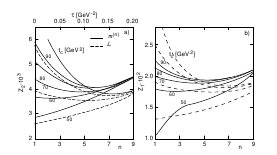
Figure 3: a) $n$- and $\tau$-dependences of the coupling $Z_{\Lambda}$ from $F_{1}$ in (90), for different values of the continuum threshold $t_{c}$. The continuous (dashed) lines come from the moments (Laplace) sum rules analysis. b) The same as in a) but from $F_{2}$.

The analysis for the residue is shown in Fig. 3 for $b=-1/5$ (we have checked that the result is insensitive to the value of $b$ between $-1$ and $+1$ though the convergence of the OPE is bad for $|b|\geq 0.5$). As can be seen in this figure, the $\tau$ or $n$ stability is reached for $t_{c}\geq 60$ GeV², while the $t_{c}$ stability starts at $t_{c}=90$GeV². We consider this range of values for our optimal estimate. Then, we obtain from the $F_{1}$ and $F_{2}$ sum rules :

$$|Z_{\Lambda}|^{2}\simeq(4.0\sim 20.0)10^{-3}\,\mbox{GeV}^{6},$$ (90)

which is quite inaccurate as other QSSR estimates of the baryon couplings in the heavy quark sector[42]–[27]. For the estimate of the $\Lambda$ mass, we use the ratios of sum rules. However, these quantities do not present an $n$/$\tau$ stability. We therefore fix the value of $n$/$\tau$ at the one where $|Z_{\Lambda}|$ is $\tau$-stable. The $t_{c}$-dependence of the $\Lambda$-mass is quite small, as shown in the Fig. 4 and we fix it in the range corresponding to the optimal value of the residue. By taking the largest range of the predictions from the $F_{1}$ and $F_{2}$ ratios of moments and Laplace sum rules, we deduce the value: $(6.86\pm 0.26)$ GeV.

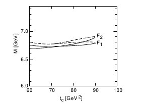
Figure 4: $t_{c}$-dependence of the $\Lambda$ mass from $F_{1}$ and $F_{2}$.

We add to the previous errors an error of about 100 MeV from $M_{b}$ and 10 MeV from the gluon condensate. Then, we deduce the final estimate :

$$M_{\Lambda}=(6.86\pm 0.28)\mbox{GeV}.$$ (91)

in good agreement with the potential model estimate in (39). This value is about $400\,\mbox{\rm MeV}$ higher than the previous result in Ref. [43], based on a particular choice of the operator.

3.5 The ${\Xi^{*}_{b}}(bbu)$ and ${\Xi^{*}_{c}}(ccu)$ masses and couplings

For a comparison with the potential model results in Table 1, let us remind the QSSR results obtained in [27]:

$$M_{\Xi^{*}_{c}}\simeq(3.58\pm 0.05)\mbox{GeV}\;\;\;\;M_{\Xi^{*}_{b}}\simeq(10.33\pm 1.09)\mbox{GeV}.$$ (92)

These predictions agree quite well with the results in Table 1 with a similar accuracy for $\Xi^{*}_{c}$. The corresponding coupling constants are:

$$|Z_{\Xi^{*}_{c}}^{2}|\simeq(3\sim 8)10^{-3}\,\mbox{GeV}^{6},\;\;\;|Z_{\Xi^{*}_{b}}^{2}|\simeq(5\sim 23)10^{-3}\,\mbox{GeV}^{6}.$$ (93)

The agreement of the different predictions between potential models and QSSR calculations of the hadron masses is a good indication of the convergence of the different theoretical estimates.

4 Semileptonic decays of the $B_{c}$ mesons

4.1 The procedures

The first investigations of the three-point functions in the framework of QCD spectral sum rules have been performed in [45] for the form factor of the pion. They have been subsequently applied to semileptonic decays of heavy–light mesons [46] and heavy–heavy mesons [41]. The first analysis of the $t$-dependence of the semileptonic form factors was given by [47]. We first shortly review the general sum rule technique for the determination of current matrix elements between heavy mesons. Let $J_{\mu}$ be the weak current in the quark sector:

$$J_{\mu}=:\bar{\psi}\gamma_{\mu}(1-\gamma^{5})Q:,$$ (94)

where $Q$ is the field for a heavy quark and $\psi$ for a light or heavy one. We shall treat here the semileptonic decays of the heavy–heavy meson $B_{c}$, with the current

$$J_{5}=(m_{b}+m_{c}):\bar{b}(i\gamma^{5})c:.$$ (95)

The decay product may be heavy–heavy ($\eta_{c}$, $J/\psi$) or heavy–light ($B_{s}$, $B_{s}^{*}$, $B$, $B^{*}$, $D$, $D^{*}$). For convenience we shall use here the method for a pseudoscalar final state with $J_{F}=(m_{\psi}+m_{Q}):\bar{\psi}(i\gamma^{5})Q:$. The starting point for the SR analysis is the three-point function ($t=(p^{\prime}-p)^{2}$):

$$\Pi_{\mu}(p,p^{\prime}) = i^{2}\int d^{4}xd^{4}y\mathrm{e}^{ip^{\prime}\cdot x-ip\cdot y}\langle 0|{\bf T}J_{F}(x)J_{\mu}(0)J_{5}^{\dagger}(y)|0\rangle$$ (96)

$$= i(p_{\mu}+p^{\prime}_{\mu})\Pi^{+}(p^{2},p^{\prime 2},t)+i(p_{\mu}-p^{\prime}_{\mu})\Pi^{-}(p^{2},p^{\prime 2},t).$$

In order to come to observables, we insert intermediate states between the weak and the hadronic current and obtain

$$\Pi_{\mu}(p,p^{\prime})={\langle 0|J_{F}|H_{F}\rangle\langle H_{F}|J_{\mu}|B_{c}\rangle\langle B_{c}|J_{5}^{\dagger}|0\rangle\over(p^{2}-M_{B_{c}}^{2})(p^{\prime 2}-M_{H_{F}}^{2})}+\hbox{\rm higher-state contributions}.$$ (97)

$H_{F}$ is the lightest meson with the quantum numbers of $J_{F}(x)$, its mass is $M_{F}$; $\langle H_{F}|J_{\mu}|B_{c}\rangle$ is the semileptonic decay matrix element we are interested in. It can be decomposed as

$$\langle H_{F}|J_{\mu}|B_{c}\rangle=F_{+}(t)(p+p^{\prime})_{\mu}+F_{-}(t)(p-p^{\prime})_{\mu}.$$ (98)

For semileptonic decays, only the form factor $F_{+}$ contributes as the contribution of $F_{-}$ is proportional to the mass squared of the lepton. The factors $\langle 0|J_{F}|H_{F}\rangle$ and $\langle B_{c}|J_{5}^{\dagger}|0\rangle$ are proportional to the decay constants (see section 3.2). The contribution of the higher states will be discussed later.

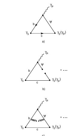
Figure 5: Different QCD contributions to the vertex functions: a) perturbative diagram, b) light-quark condensate, c) gluon condensate.

As a next step, we evaluate the three-point function $\Pi_{\mu}$ in the framework of QCD. In general one has to take into account perturbative (Fig. 5a) and non-perturbative (e.g. Fig. 5b–c) contributions. Since heavy quarks do not condense and since even for the case of a light quark in the final state the condensation of this quark (Fig. 5b) does not contribute to the three-point sum rule, only the gluon condensate (Fig. 5c) gives a non-perturbative correction. This correction is, however, expected to be very small as has been shown in [52]. Therefore, the ingredient that is dominant, by far, is the perturbative graph (Fig. 5a). The treatment of the higher power corrections thus does not play an essential role. They are taken into account by local duality [4]. If the perturbative contribution is represented by the double dispersion relation:

$$\Pi_{+}(p^{2},p^{\prime 2},t)=\int_{(m_{Q}+m_{Q^{\prime}})^{2}}^{\infty}ds\int_{(m_{\psi}+m_{Q^{\prime}})^{2}}^{\infty}ds^{\prime}{\rho_{+}^{\rm pert}(s,s^{\prime},t)\over(s-p^{2})(s^{\prime}-p^{\prime 2})},$$ (99)

one assumes that for $p^{2}$, $p^{\prime 2}$ sufficiently below the thresholds of $s$ and $s^{\prime}$ (say, $1$ GeV below) the contribution of the higher states can be well approximated by the perturbative contribution above certain thresholds $t_{c}$, $t_{c}^{\prime}$. We thus come to the sum rule:

$$\int_{(m_{Q}+m_{Q^{\prime}})^{2}}^{t_{c}}ds\int_{(m_{\psi}+m_{Q^{\prime}})^{2}}^{t_{c}^{\prime}}ds^{\prime}{\rho_{+}^{\rm pert}(s,s^{\prime},t)\over(s-p^{2})(s^{\prime}-p^{\prime 2})}+\mbox{\rm``non-pert. terms"}$$

$$\approx{\langle 0|J_{F}|H_{F}\rangle\langle B_{c}|J_{5}^{\dagger}|0\rangle F_{+}(t)\over(p^{2}-M_{B_{c}}^{2})(p^{\prime 2}-M_{H_{F}}^{2})}.$$ (100)

In order to suppress the dependence on the choice of the “continuum thresholds” $t_{c}$, $t_{c}^{\prime}$, the sum rule (100) is Borel- (Laplace-) transformed, yielding:

$$\int_{(m_{Q}+m_{Q^{\prime}})^{2}}^{t_{c}}ds\int_{(m_{\psi}+m_{Q^{\prime}})^{2}}^{t_{c}^{\prime}}ds^{\prime}\rho_{+}(s,s^{\prime},t)\mathrm{e}^{-s\tau}\mathrm{e}^{-s^{\prime}\tau^{\prime}}+\mbox{\rm``non-pert. terms"}$$

$$=\mathrm{e}^{-M_{F}^{2}\tau^{\prime}}\mathrm{e}^{-M_{B_{c}}^{2}\tau}\langle 0|J_{F}|H_{F}\rangle\langle B_{c}|J_{5}^{\dagger}|0\rangle F_{+}(t).$$ (101)

In the next step, the matrix elements $\langle 0|J_{F}|H_{F}\rangle$ and $\langle B_{c}|J_{5}^{\dagger}|0\rangle$ are expressed through sum rules as done in sections 3.1 and 3.2. By choosing the parameters $\tau$ and $\tau^{\prime}$ to be $1/2$ of the corresponding parameter in the two-point sum rule, the exponential dependence drops out, if we evaluate $F_{+}(t)$ from (101). Note that the sum rule for the two-point functions yield an expression for $|\langle 0|J_{F}|H_{F}\rangle|^{2}$ and $|\langle B_{c}|J_{5}^{\dagger}|0\rangle|^{2}$. We furthermore choose the continuum threshold the same for the two- and three-point functions, i.e. $t_{c}$ for the $B_{c}$ channel and $t_{c}^{\prime}$ for the $H_{F}$ channel. There is a very subtle point in the $t$-dependence of the perturbative double spectral function. For $t<0$ there is no problem in applying the Cutkosky rules in order to determine $\rho_{+}(s,s^{\prime},t)$ and the limits of integration. For $t>0$, which is the physical region for decays, non-Landau-type singularities appear [47, 52], which make the determination of the double spectral function very cumbersome. For finite values of $t_{c}$, $t_{c}^{\prime}$, the non-Landau singularities do not contribute to the sum rule (101) if $t$ is smaller than a certain value $t_{cr}$, which depends on $t_{c}$ and $t_{c}^{\prime}$, and hence the Cutkosky rules may be applied in a straightforward way. For the determination of the ratios, we extrapolate the $t$-dependence of that range to the full range with a cubic extrapolation.

The continuum thresholds $t_{c}$ and $t^{\prime}_{c}$ are parametrized by

$$t_{c}=(m_{Q}+m_{Q^{\prime}}+E_{c})^{2}\ \ ,\ \ t^{\prime}_{c}=(m_{Q}+m_{Q^{\prime}}+E^{\prime}_{c})^{2}\ \ .\ \$$ (102)

In many cases [5], [39], [27], [42]–[44], [47], [50], [51]:

$$E_{c}\simeq 1.\sim 2.~{}\mbox{GeV}$$ (103)

yields optimal results for the QSSR analysis. We shall use for definiteness the previous range in our analysis. In the evaluation, we do not take the (small) contribution from the gluon condensate into account and we hence come to the following sum rules :

$$F_{+}(t)={\mathrm{e}^{-M_{F}^{2}\tau^{\prime}}\mathrm{e}^{-M_{B_{c}}^{2}\tau^{\prime}}\over\langle 0|J_{F}|H_{F}\rangle\langle B_{c}|J_{5}^{\dagger}|0\rangle}\int_{(m_{Q}+m_{Q^{\prime}})^{2}}^{(m_{Q}+m_{Q^{\prime}}+E_{c})^{2}}ds\int_{(m_{\psi}+m_{Q^{\prime}})^{2}}^{(m_{Q}+m_{Q^{\prime}}+E^{\prime}_{c})^{2}}ds^{\prime}\rho_{+}(s,s^{\prime},t)\mathrm{e}^{-s\tau}\mathrm{e}^{-s^{\prime}\tau^{\prime}}.$$ (104)

For the case of a vector meson in the final state, the relevant amplitudes are given by :

$$\langle H_{F}\epsilon^{(\lambda)}|J_{\mu}|B_{c}\rangle=-iF_{0}^{A}(t)\epsilon^{*}_{\mu}+iF_{+}^{A}(t)\epsilon^{*(\lambda)}\cdot p\;(p+p^{\prime})_{\mu}$$

$$+2F_{V}(t)\epsilon_{\mu}^{\nu\rho\sigma}\epsilon^{*(\lambda)}_{\nu}p_{\rho}p^{\prime}_{\sigma}+\dots$$ (105)

The amplitudes $F_{+}$ and $F_{V}$ receive their contributions from the vector currents, while $F_{0}^{A}$ and $F_{+}^{A}$ do so from the axial-vector one. The relation between the scalar functions given in (98) and (D.12) and the ones used in Refs. [49, 47] is

$$\begin{array}[]{lclclclc}F_{+}&=&f_{+}&;&F_{0}^{A}&=&(M_{B_{c}}+M_{f})A_{1}&;\\ F^{A}_{+}&=&\displaystyle{{-A_{2}\over M_{B_{c}}+M_{V}}}&;&F_{V}&=&\displaystyle{{V\over M_{B_{c}}+M_{V}}}&.\end{array}$$ (106)

For each of the amplitudes in (105), there is a sum rule like (104), with $\rho_{+}$ replaced by $\rho_{0}^{A}$, $\rho_{+}^{A}$ and $\rho_{V}$ respectively. For completeness, we quote the relation of the amplitudes to the decay rate. In the case of the pseudoscalar final state, we have :

$${d\Gamma_{+}\over dt}={G_{F}^{2}|V_{Q\psi}|^{2}\over 192\pi^{3}M_{B_{c}}^{3}}\lambda^{3/2}(M_{B_{c}}^{2},M_{F}^{2},t)F_{+}^{2}(t),$$ (107)

while for the vector final state :

$${d\Gamma_{+}\over dt} = {G_{F}^{2}|V_{Q\psi}|^{2}\over 192\pi^{3}M_{B_{c}}^{3}}\lambda^{1/2}(M_{B_{c}}^{2},M_{F}^{2},t)$$

$$\times \left[2(F_{0}^{A})^{2}+\lambda F_{V}^{2}+{1\over 4M_{F}^{2}}\left((M_{B_{c}}^{2}-M_{F}^{2}-t)F_{0}^{A}+\lambda F_{+}^{A}\right)^{2}\right],$$

$$\lambda = \lambda(M_{B_{c}}^{2},M_{F}^{2},t).$$ (108)

4.2 Results

The principal results of the sum-rules evaluation of the form factors in (104) are collected in Table 3.

Channels	Reference	$f_{+}$	$V$	$A_{2}$	$A_{1}$
$c\bar{c}$	This paper	$0.55\pm 0.10$	$0.48\pm 0.07$	$0.30\pm 0.05$	$0.30\ 0.05$
	[41]	$0.20\pm 0.01$	$0.37\pm 0.1$	$0.27\pm 0.03$	$0.28\pm 0.01$
$b\bar{s}$	This paper	$0.60\pm 0.12$	$1.6\pm 0.3$	$0.06\pm 0.06$	$0.40\pm 0.10$
	[41]	$0.30\pm 0.05$	$2.1\pm 0.25$	$0.39\pm 0.05$	$0.35\pm 0.20$
$B\rightarrow D^{(*)}$	[52]	$0.75\pm 0.05$	$0.8\pm 0.1$	$0.68\pm 0.08$	$0.65\pm 0.10$
	[49]	$0.69$	$0.71$	$0.69$	$0.65$
	[48]	$0.62\pm 0.06$	$0.58\pm 0.03$	$0.53\pm 0.09$	$0.46\pm 0.02$

	$B_{c}\rightarrow\eta_{c}$	$B_{c}\rightarrow B_{s}$	$B_{c}\rightarrow B$	$B_{c}\rightarrow D$
	$B_{c}\rightarrow J/\psi$	$B_{c}\rightarrow B^{*}_{s}$	$B_{c}\rightarrow B^{*}$	$B_{c}\rightarrow D^{*}$
$F_{+}(0)$	$0.55\pm 0.10$	$0.60\pm 0.12$	$0.48\pm 0.14$	$0.18\pm 0.08$
$F_{V}(0)$ [GeV-1]	$0.048\pm 0.007$	$0.15\pm 0.02$	$0.11\pm 0.02$	$0.02\pm 0.01$
$F^{A}_{+}(0)$ [GeV-1]	$-0.030\pm 0.003$	$-0.005\pm 0.005$	$0.005\pm 0.005$	$0.010\pm 0.010$
$F^{A}_{0}(0)$ [GeV]	$3.0\pm 0.5$	$3.3\pm 0.7$	$1.7\pm 0.7$	$0.8\pm 0.4$
155–384	(10–75) $10^{3}$

Table 3: Comparison of semileptonic form factors for different decays. We compare the dimensionless quantities $f_{+}$, $A_{1}$, $A_{2}$, $V$ related to $F^{A}_{0}$, $F^{A}_{+}$ and $F_{V}$ through (106).

The value with the lower (resp. larger) modulus corresponds to the value of the continuum energy $E_{c}=1$GeV (resp. $2$GeV).

Channels	Reference	Rates in $10^{10}\mbox{\rm s}^{-1}$
$B_{s}l\nu$	This paper	$0.35\pm 0.10$
	[41]	$0.18$
$B^{*}_{s}l\nu$	This paper	$0.35\pm 0.10$
	[41]	$0.87$
$b\bar{s}l\nu$	This paper
	[41]
	[17]	$2.91$
$\eta_{c}l\nu$	This paper	$0.27\pm 0.07$
	[41]	$0.03$
$J/\psi l\nu$	This paper	$0.32\pm 0.08$
	[41]	$0.21$
$c\bar{c}l\nu$	This paper
	[41]
	[17]	$6.90$

Table 4: Partial decay rates for $B_{c}$ and $B^{*}_{c}$ mesons

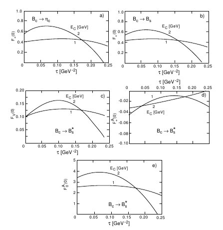
Figure 6: $\tau\simeq\tau^{\prime}$-dependence of the different form factors for $B_{c}$ semileptonic decays at zero momentum transfer for different values of the continuum threshold $E_{c}$ : a) $B_{c}\rightarrow\eta_{c}$, b) $B_{c}\rightarrow B_{s}$, c)–e) $B_{c}\rightarrow B^{*}_{s}$.

In Fig. 6, we display the result of the form factors at $t=0$ as function of $\tau$ (parameter of the initial state) $\simeq$ $\tau^{\prime}$ (parameter of the final state). It shows a weak $E_{c}$-dependence for $E_{c}$ in the range given in (103) while the $\tau$-stability is roughly about one-half of the one from the two-point correlator (see Fig. 3).

In Fig. 7,

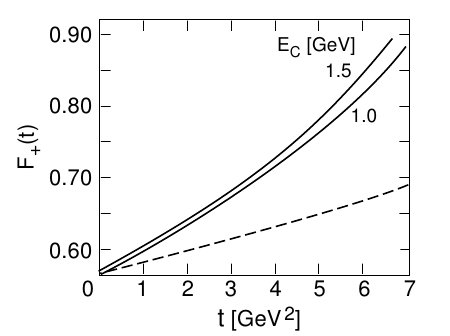
Figure 7: $t$-dependence of the $B_{c}\rightarrow\eta_{c}$ form factor: the continuous lines are the QCD predictions using a polynomial fit; the dashed line is the vector meson dominance prediction using a pole parametrization with a $B^{*}_{c}$ mass of 6.33 GeV.

we show the $t$-dependence of the form factor for the semi-leptonic decay of $B_{c}$ into $\eta_{c}$ for $E_{c}$= 1 and 1.5 GeV. The QSSR predictions with a polynomial fit are represented by the continuous lines. The result from the pole parametrization

$$F_{+}(t)={1\over 1-{t/M^{2}_{\rm pole}}}$$ (109)

is given by the dashed line assuming a vector dominance with a $B^{*}_{c}$ mass of $6.33\,$GeV. Our analysis indicates that for large t-values the QCD prediction differs notably from the pole parametrization within VDM. The same phenomena is observed in the other channels as well. For the $B_{c}$ into $J/\Psi$ semi-leptonic decay, we only quote the fitted pole masses:

$$F_{V}:\quad M_{\rm pole}\simeq 4.08\;\mbox{GeV},$$

$$F_{+}^{A}:\quad M_{\rm pole}\simeq 4.44\;\mbox{GeV},$$

$$F_{0}^{A}:\quad M_{\rm pole}\simeq 4.62\;\mbox{GeV},$$ (110)

needed for reproducing the QCD predictions.

4.3 Discussions

As mentioned above, the smallness of the non-perturbative corrections is a particular feature of the $\bar{b}c$ system. The analysis is rather an application of local duality and the continuum model than of the classical sum rules analysis as the stability of the results versus the continuum threshold is only reached if one assumes that it is the same (however a natural choice) for the two- and three-point functions. Nevertheless, we expect that the “physical” results should lie in the range spanned by the rather conservative choice of continuum thresholds, which corresponds in different other channels to the optimal results from QSSR. The choice of the continuum used in [40],[41] does not belong to this range and makes their results doubtful.

There is a considerable theoretical interest in the $t$-dependence of the form factors for the heavy–heavy to heavy–heavy decays. In [53, 54], it has been shown in realistic models that the $t$-dependence of the form factors of heavy–heavy mesons are not determined by the lowest mass in the $t$-channel (vector meson dominance), but by the size of the meson. This feature, which is obviously present in potential models, is also visible in the sum rule analysis, as can be seen from Fig. 7. The $t$-dependence is indeed much stronger than predicted by vector meson dominance. Experimentally, it would be important to verify this deviation from a hadronic effective theory.

5 Conclusions

We have combined in this paper potential models and QCD spectral sum rules for studying the properties of hadrons with charm and beauty. We present in section 2 the results from potential models with the emphasis on the accuracy of the models for predicting the hadron masses. In section 3, we present the QCD spectral sum rules estimates where we show that the values of the decay constants can come out quite accurately once we use the meson masses from potential models and once we understand better the Wilson coefficients in the Operator Product Expansion of the correlators. Indeed, we show explicitly here how the Wilson coefficients of the gluon condensates already contain the ones of the heavy quark and heavy quark-gluon mixed condensates. This point has been a source of confusion and uncertainties in the past. Finally, we use in section 4 vertex sum rules in order to study the form factors of the $B_{c}$ semileptonic decays. In particular, we show that their $t$-dependence deviates notably from the one predicted by vector meson dominance.

6 Appendix

As anticipated in Sec. 3.1, dispersion relations such as

$$C_{G^{2}}(q^{2})={1\over\pi}\int_{0}^{\infty}{dt\,{\rm Im}\,C_{G^{2}}(t)\over t-q^{2}}$$ (111)

require adding to (48) $\delta$-functions and derivatives of $\delta$-functions in order for them to be finite (and correct). The reason for that should be clear by noting that (48) behaves as $[t-(m_{b}+m_{c})^{2}]^{-5/2}$ near theshold, thus giving a divergent contribution to (111). The evaluation of these extra terms can be rather cumbersome. Here we present a simpler alternative modification of (111) which one can prove without much effort. For the sake of simplicity, we illustrate the method with the $\langle G^{2}\rangle$ contribution. Let us start by explicitly substituting (48) in (111):

$$C_{G^{2}}(q^{2})=\!\!{1\over\pi}\!\!\int_{(m_{b}+m_{c})^{2}}^{\infty}\!\!\!\!\!\!\!dt{-\alpha_{s}m_{b}m_{c}\,t\,\left(t\!-\!m_{b}^{2}\!\!-\!\!m_{b}m_{c}\!\!-\!\!m_{c}^{2}\right)\over 2\,(t\!-\!q^{2})\,[t\!-\!(m_{b}\!-\!m_{c})^{2}]^{3/2}}\times{[t\!-\!(m_{b}\!+\!m_{c})^{2}]^{-5/2}}.$$ (112)

Next, we separate the singular power of $t\!-\!(m_{b}\!+\!m_{c})^{2}$, i.e. the factor ${[t\!-\!(m_{b}\!+\!m_{c})^{2}]^{-5/2}}$ in (112), from the analytic portion and compute its Taylor series in powers of $t\!-\!(m_{b}\!+\!m_{c})^{2}$ up to order one. Higher order terms are innecessary since they would give a convergent contribution to (112) near theshold. The desired Taylor series is ($-q^{2}=Q^{2}>0$):

$$- {\alpha_{s}\sqrt{m_{b}m_{c}}\over 16[Q^{2}+(m_{b}+m_{c})^{2}]}\Bigg{\{}(m_{b}+m_{c})^{2}+{t-(m_{b}+m_{c})^{2}\over 8m_{b}m_{c}[Q^{2}+(m_{b}+m_{c})^{2}]}$$ (113)

$$\times \Big{[}5(m_{b}+m_{c})^{4}+Q^{2}\left(5m_{b}^{2}+18m_{b}m_{c}+5m_{c}^{2}\right)\Big{]}\Bigg{\}}.$$

Obviously, by subtracting eq.(113) times $[t-(m_{b}+m_{c})^{2}]^{-5/2}$ from the integrand of (112) we obtain a result which is $O\{[t-(m_{b}+m_{c})^{2}]^{-1/2}\}$. Thus, this difference can be integrated as in (111). This is precisely the modification of (111) that we are looking for. So, we finally have

$$C_{G^{2}}(q^{2})\!\!\!\! = \!\!\!\!{1\over\pi}\int_{(m_{b}+m_{c})^{2}}^{\infty}\!\Bigg{\{}\!\!-{\alpha_{s}m_{b}m_{c}\,t\,\left(t\!-\!m_{b}^{2}\!-\!m_{b}m_{c}\!-\!m_{c}^{2}\right)\over 2\,(Q^{2}\!+\!t)\;[t\!-\!(m_{b}\!-\!m_{c})^{2}]^{3/2}}$$

$$- \!\!{\alpha_{s}\sqrt{m_{b}m_{c}}}\Bigg{\{}{(m_{b}\!+\!m_{c})^{2}[t\!-\!(m_{b}\!+\!m_{c})^{2}]\over 16[Q^{2}+(m_{b}+m_{c})^{2}]^{2}}-{1\over 16[Q^{2}\!+\!(m_{b}\!+\!m_{c})^{2}]}$$

$$\times \Big{[}(m_{b}\!+\!m_{c})^{2}+{(5m_{b}^{2}\!+\!18m_{b}m_{c}\!+\!5m_{c}^{2})[t-(m_{b}+m_{c})^{2}]\over 8m_{b}m_{c}}\Big{]}\Bigg{\}}\Bigg{\}}$$

$$\times {dt\over[t\!-\!(m_{b}\!+\!m_{c})^{2}]^{5/2}}.$$

We have explicitely checked that (6) agrees with [5]. An entirely analogous procedure can be followed to obtain the dispersion relation for $C_{G^{3}}$. One has

$$C_{G^{3}}(q^{2}) = {1\over\pi}\int_{\SS}^{\infty}{dt\over[t-\SS]^{9/2}}\Bigg{\{}{\alpha_{s}m_{b}m_{c}\;t\over 6\;(t+Q^{2})\,[t-(m_{b}-m_{c})^{2}]^{7/2}}$$

$$\times \Big{\{}3t^{4}-2(3m_{b}^{2}+2m_{b}m_{c}+3m_{c}^{2})t^{3}$$

$$+ (5m_{b}^{3}m_{c}+18m_{b}^{2}m_{c}^{2}+5m_{b}m_{c}^{3})\;t^{2}$$

$$+ 2(3m_{b}^{6}+m_{b}^{5}m_{c}-6m_{b}^{4}m_{c}^{2}-6m_{b}^{3}m_{c}^{3}-6m_{b}^{2}m_{c}^{4}+m_{b}m_{c}^{5}+3m_{c}^{6})\;t$$

$$- 3(m_{b}^{8}+m_{b}^{7}m_{c}-m_{b}^{5}m_{c}^{3}-2m_{b}^{4}m_{c}^{4}-m_{b}^{3}m_{c}^{5}+m_{b}m_{c}^{7}+m_{c}^{8})\Big{\}}$$

$$- \alpha_{s}\sqrt{m_{b}m_{c}}\left\{{-7\Sigma^{4}\,(t-\SS)^{3}\over 192\,(Q^{2}+\SS)^{4}}\right.$$

$$+ \left[{7\SS\,(t-\SS)^{2}\over 192}+{A\,(t-\SS)^{3}\over 1536m_{b}m_{c}}\right]{\SS\over(Q^{2}+\SS)^{3}}$$

$$+ \left[{-7\Sigma^{4}\,(t-\SS)\over 192}-{\SS\,A\,(t-\SS)^{2}\over 1536m_{b}m_{c}}+{B\,(t-\SS)^{3}\over 24576m_{b}^{2}m_{c}^{2}}\right]{1\over(Q^{2}+\SS)^{2}}$$

$$+ \left.\left[{7\Sigma^{4}\over 192}+{\SS\,A\,(t-\SS)\over 1536m_{b}m_{c}}-{B\,(t-\SS)^{2}\over 24576m_{b}^{2}m_{c}^{2}}-{C\,(t-\SS)^{3}\over 196608m_{b}^{3}m_{c}^{3}}\right]{1\over Q^{2}+\SS}\right\}\Bigg{\}},$$

where we have introduced the notation:

$$\Sigma = m_{b}+m_{c}$$

$$A = 51m_{b}^{2}+166m_{b}m_{c}+51m_{c}^{2}$$

$$B = 31m_{b}^{4}-836m_{b}^{3}m_{c}-1862m_{b}^{2}m_{c}^{2}-836m_{b}m_{c}^{3}+31m_{c}^{4}$$

$$C = 277m_{b}^{4}+596m_{b}^{3}m_{c}-514m_{b}^{2}m_{c}^{2}+596m_{b}m_{c}^{3}+277m_{c}^{4}.$$ (116)

The result is seen to agree with previous calculations of the (real) part of $C_{G^{3}}$ in the case $m_{b}=m_{c}$ [36]. Note that from (6) and (6) it is straightforward to calculate both the Borel- (Laplace-) transform of $C_{G^{2}}$ and $C_{G^{3}}$ and their moments since the dependence on $Q^{2}$ is through $(Q^{2}+t)^{-n}$ or/and $(Q^{2}+\SS)^{-n}$.

References

- [1] A. De Rújula et al., Proc. LHC Workshop, Aachen 1990, CERN 90-10,Vo 2, p.201.
- [2] E. Eichten and F. Feinberg, Phys. Rev. D23 (1981) 2724.
- [3] S. Narison, Phys. Lett. B210 (1988) 238.
- [4] M.A. Shifman, A.I. Vainshtein and V.I. Zakharov, Nucl. Phys. B147 (1979) 385, 448.
- [5] For a recent review, see e.g: S. Narison, Lecture Notes in Physics, Vol. 26, QCD Spectral Sum Rules (World Scientific, Singapore, 1989) and references therein;
- [6] For reviews see e.g. H. Georgi, Proceedings of TASI-91 (World Scientific, Singapore, 1991), edited by R.K. Ellis et al.; N. Isgur and M. Wise, Proceedings of Heavy Flavours (World Scientific, Singapore, 1992), edited by A. Buras and M. Lindner; T. Mannel, Talk given at the 5th International Symposium on Heavy Flavours, Montreal, Canada, 6-10 June 1993, CERN preprint TH-7052/93 (1993).
- [7] C. Quigg and J.L. Rosner, Phys. Rep. 56 (1979) 167.
- [8] H. Grosse and A. Martin, Phys. Rep. 60 (1979) 341.
- [9] A. Martin, in Proc. Int. Universitätswochen für Kernphysik, Schladming, Austria, 1986, ed. H. Latal and H. Mittner (Springer Verlag, Berlin, 1987).
- [10] J.-M. Richard, Phys. Rep. 212 (1992) 1.
- [11] H. Grosse and A. Martin, book in preparation.
- [12] See, e.g., W. Thirring, A Course in Mathematical Physics, Vol. 3 (Springer Verlag, Berlin 1981).
- [13] R.A. Bertlmann and A. Martin, Nucl. Phys. B168 (1980) 111.
- [14] Particle Data Group, Review of Particle Properties, Phys. Rev. D45 (1992) 1; D46 (1992) 5210 (E).
- [15] A. Martin, in Heavy Flavours and High Energy Collisions in the 1–100 TeV Range, Proc. Erice Workshop (1988), ed. A. Ali and L. Cifarelli (Plenum, New York, 1989).
- [16] S.S. Gershtein, V.V. Kiselev, A.K. Likhoded, S.R. Slabospitskiǐ and A.V. Tkabladze, Sov. J. Nucl. Phys. 48 (1988) 327.
- [17] E. Eichten and C. Quigg, Workshop on Beauty Physics at Colliders, to appear in the Proceedings; Fermilab-pub-91/032-T (1994); C. Quigg, Fermilab-Conf-93/265-T (1993).
- [18] S. Godfrey and N. Isgur, Phys. Rev. D32 (1985) 189.
- [19] M. Lusignoli and M. Masetti, Z. Phys. C51 (1991) 549.
-
[20]
S. Nussinov, Phys. Rev. Lett. 52 (1984) 966;
J.-M. Richard and P. Taxil, Phys. Rev. Lett. 54 (1985) 847;
E. Lieb, Phys. Rev. Lett. 54 (1985) 1987;
A. Martin, J.-M. Richard and P. Taxil, Phys. Lett. 176B (1986) 224. - [21] A. Martin, Phys. Lett. B287 (1992) 251.
- [22] R.L. Hall and H.R. Post, Proc. R. Phys. Soc. 90 (1967) 381.
- [23] J.-L. Basdevant, A. Martin and J.-M. Richard, Nucl. Phys. B343 (1990) 69.
- [24] S. Fleck and J.-M. Richard, Progr. Theor. Phys. 82 (1989) 760.
- [25] J.-M. Richard and P. Taxil, Phys. Lett. B128 (1983) 453.
- [26] OPAL Collaboration, Contribution to the 1993 EPS Conference, Marseille, July 1993; we thank Fabienne Ledroit for this information.
- [27] E. Bagan, M. Chabab and S. Narison, Phys. Lett. B306 (1993) 350.
- [28] J. Hiller, J. Sucher and G. Feinberg, Phys. Rev. A18 (1978) 2399.
- [29] I. Cohen and H.J. Lipkin, Phys. Lett. B106 (1981) 119.
-
[30]
D. Broadhurst and S.C. Generalis,
Open University preprint, OUT 4102-8 (1982) (unpublished); S.C. Generalis,
Ph.D Thesis, OUT 4102-13 (1982) (unpublished),
J. Phys. G16 (1990) 785, 367. - [31] V.A. Novikov et al., Fortsch. Phys. 32 (1984) 585.
- [32] M. Jamin and M. Munz, Z. Phys. C60 (1993) 569.
- [33] D. J. Broadhurst and S. C. Generalis, Phys. Lett. B139 (1984) 85; B142 (1984) 75; B165 (1985) 175
- [34] S. Narison, Z. Phys. C55 (1992) 671.
- [35] S. N. Nikolaev and A. V. Radyushkin, Nucl. Phys. B213 (1983) 285.
- [36] E. Bagan, J. I. Latorre and P. Pascual, Z. Phys. C32 (1984) 75.
- [37] V.A. Novikov et al., Nucl. Phys. B237 (1984) 525.
- [38] S. Narison, Phys. Lett. B198 (1987) 104 and B308 (1993); Talk given at the Third –Charm Factory Workshop, 1–6 June 1993, Marbella, Spain, CERN preprint TH-7042/93 (1993).
- [39] S. Narison and M. Zalewski, Phys. Lett. B320 (1994) 369.
- [40] C.A. Dominguez, K. Schilcher and Y.L. Wu, Phys. Lett. B298 (1993) 190.
- [41] P. Colangelo, G. Nardulli and N. Paver, Z. Phys. C57 (1993) 43.
- [42] E. Bagan, M. Chabab, H. G. Dosch and S. Narison, Phys. Lett. B287 (1992) 176.
- [43] E. Bagan, M. Chabab, H.G. Dosch and S. Narison, Phys. Lett. B301 (1993) 243.
- [44] E. Bagan, M. Chabab, H.G. Dosch and S. Narison, Phys. Lett. B278 (1992) 367.
- [45] B.L. Ioffe and A.V. Smilga, Phys. Lett. B114 (1982) 353; Nucl. Phys. B216 (1983) 373.
- [46] A. Ovchinnikov and V.A. Slobodenyuk, Z. Phys. C44 (1989) 433. V.N. Baier and A.G. Grozin, Z. Phys. C47 (1990) 669.
- [47] P. Ball, V.M. Braun and H.G. Dosch, Phys. Rev. D44 (1991) 3567.
- [48] S. Narison, Phys. Lett. B283 (1992) 384.
- [49] M. Bauer, B. Stech and M. Wirbel, Z. Phys. C29 (1985) 637.
- [50] E. Bagan, P. Ball and P. Gosdzinsky, Phys. Lett. B301 (1993) 101.
- [51] M. Neubert, Phys. Rev. D45 (1992) 2451 and D46 (1992) 1076.
- [52] P. Ball, Phys. Rev. D48 (1993) 3190.
- [53] R.L. Jaffe, Phys. Lett. B245 (1990) 221.
- [54] R.L. Jaffe and P.F. Mende, Nucl. Phys. B369 (1992) 189.