CERN–TH.7151/94

FTUV/94–6

IFIC/94–3

QCD corrections to inclusive $\Delta S=1,2$ transitions
at the next-to-leading order

Matthias Jamin
Theory Division, CERN, CH–1211 Geneva 23, Switzerland
and

Antonio Pich
Departament de Física Teòrica, Universitat de València
and IFIC, Centre Mixte Universitat de València – CSIC
E–46100 Burjassot, València, Spain

Abstract

The 2–point functions for $\Delta S=1$ current-current and QCD-penguin operators, as well as for the $\Delta S=2$ operator, are calculated at the next-to-leading order. The calculation is performed in two different renormalization schemes for $\gamma_{5}$, and the compatibility of the results obtained in the two schemes is verified. The scale- and scheme-invariant combinations of spectral 2–point functions and corresponding Wilson-coefficients are constructed and analyzed. For $\Delta S=1$, the QCD corrections to the CP-conserving part, dominated by current-current operators, are 40%–120% at $q^{2}=\left(1-3\,\mbox{\rm GeV}\right)^{2}$, whereas the correction to the imaginary part, mainly coming from the penguin operator $Q_{6}$, are 100%–240%. The large size of the gluonic corrections to current-current operators provides a qualitative understanding of the observed enhancement of $\Delta I=1/2$ transitions. In the $\Delta S=2$ sector the QCD corrections are quite moderate ($\approx-20\%$).

CERN–TH.7151/94

February 1994

1 Introduction

Recent years have witnessed considerable improvement in Standard Model calculations of non-leptonic weak decays. In particular, the effective Hamiltonians for flavour-changing $\Delta F=1$ [1, 2, 3, 4] as well as $\Delta F=2$ [5, 6] transitions were calculated at the next-to-leading order (NLO) in renormalization group (RG) improved perturbation theory. The necessary computations included the determination of 2–loop anomalous dimension matrices for current-current, QCD-penguin, and electroweak penguin operators [1, 2, 7, 8, 9, 10, 11]. The benefit from such calculations is the following:

• the size of the NLO short distance corrections to the coefficient functions was obtained,

• this allowed an estimation of the scale down to which RG evolution is possible, before perturbation theory breaks down, to be around $1\,\mbox{\rm GeV}$,

• only a NLO calculation allows for a meaningful use of the QCD scale $\Lambda_{\overline{MS}}$, extracted for example in deep inelastic scattering, $\tau$ decay or LEP experiments,

• and it made possible to attack the question of the dependence of coefficient functions on the renormalization scheme, e.g. the definition of $\gamma_{5}$ in an arbitrary space-time dimension, which first appears at the next-to-leading order.

Sadly enough, this is not the whole story. In order to fully calculate the decay amplitude for a certain process, we also need to know the matrix elements of the operators appearing in the effective Hamiltonian, between the hadronic initial and final states. This part is much more difficult, for it involves non-perturbative dynamics at low energies. Methods to attempt this involved task include lattice gauge theory [12, 13, 14], $1/N$-expansion [15, 16, 17], chiral perturbation theory [18, 19], QCD sum rules [20, 21, 22, 23, 24, 25, 26], and mixed approaches involving functional integration of quark fields [26]. A strategy to obtain the matrix elements for $\Delta S=1$ decays at NLO as far as possible from experimental data was also advocated in ref. [4].

All these methods suffer from more or less severe drawbacks. Although the lattice could eventually become the ultimate tool for the calculation of matrix elements, the precision of present lattice results is still very poor. $1/N$-expansion and chiral perturbation theory are not yet directly related to the fundamental QCD Lagrangian, and therefore, a sound matching of matrix elements calculated in one of these methods and the coefficient functions, obtained in perturbation theory, is still not possible. The bridge between the effective low-energy chiral Lagrangian and the underlying QCD theory can be built with functional bosonization techniques [26], or using QCD sum rules to relate the two energy regimes [20, 21, 22, 23, 24, 25, 26]. Unfortunately, the present determinations are not very accurate. Finally, there is not enough experimental information to obtain all matrix elements, say for $K\rightarrow\pi\pi$ decays, from the phenomenological method of ref. [4].

The problem becomes much easier at the inclusive level, where the properties of the non-leptonic effective weak Hamiltonian can be analyzed within QCD [20, 21, 22, 23, 24, 26]. Given, for instance, the short-distance $\Delta S=1$ Hamiltonian [2, 4]

$${\cal H}^{\Delta S=1}_{\mbox{\rm\scriptsize eff}}\;=\;{G_{F}\over\sqrt{2}}\,V_{ud}^{\phantom{*}}V_{us}^{*}\sum_{i}C_{i}(\mu^{2})\,Q_{i}\,,$$ (1.1)

obtained through the operator product expansion, one considers the 2–point function

$$\Psi^{\Delta S=1}(q^{2}) \equiv i\int\!dx\,e^{iqx}\,\big{<}0|\,T\{\,{\cal H}^{\Delta S=1}_{\mbox{\rm\scriptsize eff}}(x)\,{\cal H}^{\Delta S=1}_{\mbox{\rm\scriptsize eff}}(0)^{\dagger}\}|0\big{>}$$ (1.2)

$$= \left({G_{F}\over\sqrt{2}}\right)^{2}\left|V_{ud}^{\phantom{*}}V_{us}^{*}\right|^{2}\,\sum_{i,j}\,C_{i}(\mu^{2})\,C_{j}^{*}(\mu^{2})\,\Psi_{ij}(q^{2})\,.$$

This vacuum-to-vacuum correlator can be studied with perturbative QCD methods, allowing for a consistent combination of Wilson-coefficients $C_{i}(\mu^{2})$ and 2–point functions of the 4–quark operators, $\Psi_{ij}$, in such a way that the renormalization scheme and scale dependences exactly cancel (to the computed order). The associated spectral function $\frac{1}{\pi}\mbox{\rm Im}\Psi^{\Delta S=1}(q^{2})$ is a quantity with definite physical information. It describes in an inclusive way how the weak Hamiltonian couples the vacuum to physical states of a given invariant mass. General properties like the observed enhancement of $\Delta I=1/2$ transitions can be then rigorously analyzed at the inclusive level.

A detailed analysis of 2–point functions associated with $\Delta S=1$ and $\Delta S=2$ operators was presented in ref. [26], where the ${\cal O}(\alpha_{s})$ corrections to the corresponding correlators $\Psi_{ij}$ were calculated. The NLO corrections to the $\Delta I=1/2\,$ 2–point functions were found to be very large [26], confirming the QCD enhancement obtained in a previous approximate calculation [24]. The results of ref. [26] were, however, incomplete because the NLO corrections to the Wilson-coefficients of penguin operators were still missing. With the progress achieved for the Wilson-coefficient functions mentioned above, we are now in a position to match matrix elements and coefficient functions consistently at NLO.

To get a sensible result, we obviously need to use the same renormalization scheme conventions on both sides of the calculation. Unfortunately, for technical reasons, different bases of operators have been used in the 2–point function and Wilson-coefficient calculations. In order to avoid ambiguities coming from the definition of $\gamma_{5}$ in $d\not=4$ dimensions, a set of colour-singlet 4–quark operators was used in ref. [26] to perform the 2–point-function calculation; the computation was done with dimensional regularization and a naively anticommuting $\gamma_{5}$ (NDR scheme). While that is fine in the leading logarithmic approximation, the basis of colour-singlet operators does not close under renormalization at the NLO. The Fierz-transformations, which are needed to relate some of the operators in the process of renormalization, are broken by ${\cal O}(\alpha_{s})$ corrections, and additional contributions have to be taken into account. For this reason, we shall reconsider the calculation of the 2-point functions of 4–quark operators in this work.

We shall use the same basis of operators which has been taken for the calculation of the Wilson-coefficients, so that we can directly incorporate the results of refs. [2, 7, 8, 11]. The presence of colour-non-singlet operators in this basis gives rise to $\gamma_{5}$ complications in the 2–point-function evaluation. Like for the calculation of the anomalous dimension matrices in refs. [2, 7, 8, 11], we shall perform the calculation in two different schemes for $\gamma_{5}$, to have explicit tests on our result. A direct computation with a naively anticommuting $\gamma_{5}$ is not possible, since two diagrams include traces of odd numbers of $\gamma_{5}$; but we shall show, how nevertheless a result in the NDR scheme can be obtained. For the second computation, the consistent definition of a non-anticommuting $\gamma_{5}$ in arbitrary dimensions according to ’t Hooft and Veltman (HV scheme) [27, 28, 7] is used.

In sect. 2, we shall discuss the general structure of 2–point functions of 4–quark operators. As a first step towards the explicit calculation for the $\Delta S=1$ case, in sect. 3, the 2–point functions of current-current operators are computed, and the full set including QCD-penguins is presented in sect. 4. A numerical analysis of the results is given in sect. 5. In sect. 6, we evaluate the 2–point function for the $\Delta S=2$ operators. A comparison with the results of ref. [26], together with some concluding remarks, is finally given in sect. 7.

2 General structure

As a first step, let us discuss the general structure of the 2–point functions of 4–quark operators and their renormalization. The bare 2–point function $\Psi^{B}(q^{2})$ is defined by

$$\Psi^{B}(q^{2})\;\equiv\;i\int\!dx\,e^{iqx}\,\big{<}0|\,T\{\,Q^{B}(x)\,Q^{B^{\dagger}}(0)\}|0\big{>}\,.$$ (2.1)

$Q(x)$ can either be a single operator, or a vector of 4–quark operators, in which case $\Psi^{B}(q^{2})$ is a symmetric matrix.

Keeping only relevant terms up to next-to-leading order in $\alpha_{s}$, and working with dimensional regularization, the regularized, but yet unrenormalized 2–point function $\Psi^{R}(q^{2},\mu^{2})$ has an expansion in $\varepsilon$ ($d=4+2\varepsilon$),

$$\Psi^{R}(q^{2},\mu^{2}) = -\,\frac{(q^{2})^{4}}{(4\pi)^{6}}\,\biggl{\{}\,\biggl{(}\frac{-q^{2}}{\mu^{2}}\biggr{)}^{3\varepsilon}\frac{1}{3\varepsilon}\,\Big{[}\,A+B\varepsilon+\ldots\Big{]}$$

$$\hskip 21.9086pt+\,\frac{\alpha_{s}}{\pi}\biggl{(}\frac{-q^{2}}{\mu^{2}}\biggr{)}^{4\varepsilon}\frac{1}{4\varepsilon^{2}}\,\Big{[}\,C+D\varepsilon+\ldots\Big{]}+{\cal O}(\alpha_{s}^{2})\,\biggr{\}}\,.$$ (2.2)

$\mu^{2}$ is a renormalization scale in the ${\overline{MS}}$ scheme, that is, we have redefined the scale of dimensional regularization $\nu^{2}$ to be $\exp(\gamma_{E})\,\mu^{2}/(4\pi)$, where $\gamma_{E}$ is Euler’s constant, so that only poles in $\varepsilon$ have to be subtracted. Our main goal will be to calculate the four matrices $A$, $B$, $C$, and $D$.

The renormalized 2–point function is given by

$$\Psi(q^{2},\mu^{2})\;=\;R_{\overline{MS}}\,\Big{[}\,Z^{-1}\,\Psi^{R}(q^{2},\mu^{2})\,\big{(}Z^{-1}\big{)}^{T}\,\Big{]}\,,$$ (2.3)

where $Z$ is the renormalization matrix of the 4–quark operators, $Q^{B}\equiv Z\,Q$, and $R_{\overline{MS}}$ means that additional poles in $\varepsilon$, stemming from the operator product, need to be subtracted. In the minimal subtraction scheme, $Z$ has the general expansion

$$Z\;=\;1+\sum_{k=1}^{\infty}\Big{(}\frac{\alpha_{s}}{\pi}\Big{)}^{k}\sum_{n=1}^{k}\frac{Z_{n}^{(k)}}{\varepsilon^{n}}\,.$$ (2.4)

The anomalous dimension matrix of 4–quark operators is defined through

$$\gamma\;\equiv\;Z^{-1}\mu\,\frac{dZ}{d\mu}\,\biggr{|}_{\varepsilon=0}\;=\;\gamma^{(1)}\,\frac{\alpha_{s}}{\pi}+\gamma^{(2)}\,\Big{(}\frac{\alpha_{s}}{\pi}\Big{)}^{2}+\ldots\,.$$ (2.5)

Inserting the expansion for $Z$, eq. (2.4), we find

$$\gamma^{(1)}\;=\;2\,Z_{1}^{(1)}\,,\qquad\gamma^{(2)}\;=\;4\,Z_{1}^{(2)}\,,\qquad Z_{2}^{(2)}\;=\;\frac{1}{4}\,Z_{1}^{(1)}\Big{(}\,2\,Z_{1}^{(1)}-\beta_{1}\,\Big{)}\,.$$ (2.6)

Here, $\beta_{1}=-\,(11N-2f)/6$ is the leading coefficient of the $\beta$–function, $N$ and $f$ being the number of colours and flavours respectively. For the operators which mediate $\Delta S=1$ transitions, and shall be our interest for most part of the paper, the leading order anomalous dimension matrix is known already since a long time [29, 30, 31, 32, 33]. However, the full next-to-leading order matrix has only been obtained recently [1, 2, 7, 8, 11]. To make contact with the notation of refs. [2, 8], we note that

$$\gamma^{(1)}\;=\;\frac{1}{4}\,\gamma_{BJLW}^{(0)}\,,\qquad\hbox{and}\qquad\gamma^{(2)}\;=\;\frac{1}{16}\,\gamma_{BJLW}^{(1)}\,.$$ (2.7)

Using the results of eq. (2.6), together with eq. (2.4), up to non-logarithmic corrections the renormalized 2–point function turns out to be

$$\Psi(q^{2},\mu^{2})\;=\;-\,\frac{(q^{2})^{4}}{(4\pi)^{6}}\,\biggl{\{}\,A\,L+\frac{\alpha_{s}}{\pi}\,\biggl{[}\,\frac{1}{2}\,CL^{2}+XL\,\biggr{]}\,\biggr{\}}\,,$$ (2.8)

where $L=\ln(-q^{2}/\mu^{2})$, and

$$X\;=\;D-\frac{1}{2}\,\Big{(}\,\gamma^{(1)}B+B\,\gamma^{(1)^{T}}\,\Big{)}\,.$$ (2.9)

Because of renormalizability, it also follows that

$$C\;=\;\frac{1}{2}\,\Big{(}\,\gamma^{(1)}A+A\,\gamma^{(1)^{T}}\,\Big{)}\,.$$ (2.10)

For the rest of this work, we shall only be concerned with the spectral function (the imaginary part of the 2–point function) which is directly related to physical quantities:

$$\Phi(s,\mu^{2})\;\equiv\;\frac{1}{\pi}\,\mbox{\rm Im}\,\Psi(q^{2},\mu^{2})\;=\;\theta(s)\,\frac{s^{4}}{(4\pi)^{6}}\,\biggl{\{}\,A+\frac{\alpha_{s}}{\pi}\,\biggl{[}\,C\ln{\biggl{|}\frac{s}{\mu^{2}}\biggr{|}}+X\,\biggr{]}\,\biggr{\}}\,,$$ (2.11)

with $s\equiv q^{2}$. It is straightforward to see that $\Phi(s,\mu^{2})$ satisfies a homogeneous renormalization group equation (RGE),

$$\mu\,\frac{d}{d\mu}\,\Phi(s,\mu^{2})+\gamma\,\Phi+\Phi\,\gamma^{T}\;=\;0\,.$$ (2.12)

This implies that

$$\widehat{\Phi}(s)\;\equiv\;C^{T}(\mu^{2})\,\Phi(s,\mu^{2})\,C^{*}(\mu^{2})$$ (2.13)

is a renormalization group invariant quantity, with $C(\mu^{2})$ being the Wilson-coefficient function of the 4–quark operators, which satisfies the RGE

$$\biggl{\{}\,\mu\,\frac{d}{d\mu}-\gamma^{T}\,\biggr{\}}\,C(\mu^{2})\;=\;0\,.$$ (2.14)

At the next-to-leading order, the coefficient function for $\Delta S=1$ operators can be found in refs. [2, 3, 4]. The scale- and scheme-independence of $\widehat{\Phi}$ should be clear, because this function is just proportional to the physical spectral function ${1\over\pi}\mbox{\rm Im}\Psi^{\Delta S=1}(s)$. The scheme independence of ${\cal H}^{\Delta S=1}_{\mbox{\rm\scriptsize eff}}$ is carried over to the 2–point function.

We can easily sum up the next-to-leading logarithms in the 2–point function by setting $\mu^{2}=s$, yielding

$$\Phi(s)\;=\;\theta(s)\,\frac{s^{4}}{(4\pi)^{6}}\,\biggl{\{}\,A+\frac{\alpha_{s}(s)}{\pi}\,X\;\biggr{\}}\,,\quad\hbox{and}\quad\widehat{\Phi}(s)\;=\;C^{T}(s)\,\Phi(s)\,C^{*}(s)\,.$$ (2.15)

Like the Wilson-coefficient function, also the spectral function at the next-to-leading order, in particular the matrices $B$ and $D$, depend on the renormalization scheme. If the renormalization matrices in two schemes $Z_{a}$ and $Z_{b}$ are related by a finite shift,

$$Z_{a}\;=\;Z_{b}\,\biggl{[}\,1+\frac{\alpha_{s}}{\pi}\,\Delta r\,\biggr{]}\,,$$ (2.16)

we find the following relation between $X$ in the two schemes,

$$X_{b}\;=\;X_{a}+\Delta r\,A+A\,\Delta r^{T}\,.$$ (2.17)

Together with the scheme dependence of the Wilson-coefficient functions (eq. (3.6) of ref. [4]),

$$C_{b}(\mu^{2})\;=\;\biggl{[}\,1-\frac{\alpha_{s}}{\pi}\,\Delta r^{T}\,\biggr{]}\,C_{a}(\mu^{2})\,,$$ (2.18)

it is a trivial check that $\widehat{\Phi}(s)$ is indeed scheme-independent up to ${\cal O}(\alpha_{s}^{2})$.

3 Current-current operators

As an introductory example, we shall first calculate the 2–point function of the $\Delta S=1$ current-current operators, before embarking on the full set including penguins:

$$Q_{1}\;=\;\left(\bar{s}_{\alpha}u_{\beta}\right)_{\rm V-A}\left(\bar{u}_{\beta}d_{\alpha}\right)_{\rm V-A}\,,\qquad Q_{2}\;=\;\left(\bar{s}u\right)_{\rm V-A}\left(\bar{u}d\right)_{\rm V-A}\,,$$ (3.1)

where $\alpha$, $\beta$ denote colour indices ($\alpha,\beta=1,\ldots,N$) and the colour indices have been omitted for the colour singlet operator $Q_{2}$. $(V-A)$ refers to $\gamma_{\mu}(1-\gamma_{5})$. This basis closes under renormalization if penguin operators are neglected.

In the course of the calculation, it will become useful to also study 2–point functions of the Fierz-transformed operators

$$\widetilde{Q}_{1}\;=\;\left(\bar{s}d\right)_{\rm V-A}\left(\bar{u}u\right)_{\rm V-A}\,,\qquad\widetilde{Q}_{2}\;=\;\left(\bar{s}_{\alpha}d_{\beta}\right)_{\rm V-A}\left(\bar{u}_{\beta}u_{\alpha}\right)_{\rm V-A}\,,$$ (3.2)

and mixtures of the bases (3.1) and (3.2). Since these mixtures do not close under renormalization, we will have to include evanescent operators. This will be discussed in detail below.

The calculation of the 2–point function requires the evaluation of the leading order 3–loop diagrams of fig. 1 and the next-to-leading 4–loop diagrams of fig. 2. The results of this evaluation are summarized in tables 1 and 2, and will be discussed in great detail in the following. A straightforward inspection reveals that the topology 2e contains traces with an odd number of $\gamma_{5}$’s. Actually, there are two diagrams of type 2e: one with the fermion lines in the upper and lower loop circulating in opposite directions, denoted by 2e, and one with the same direction, denoted by 2e’. These cannot directly be calculated in renormalization schemes with a naively anticommuting $\gamma_{5}$. For this reason, and also to make direct contact with the NLO calculation of the Wilson-coefficient function [2, 3, 4], we shall perform the calculation with a non-anticommuting $\gamma_{5}$, originally due to ’t Hooft and Veltman [27, 28, 7], and in addition we present a way to nevertheless obtain results in the NDR scheme.

Table 1: Results for the lowest-order diagrams of fig. 1.

Diagram	1a	1b
$A$	$\frac{4}{45}$	$\frac{4}{45}$
$B^{NDR}$	$-\frac{653}{675}$	$-\frac{593}{675}$
$B^{HV}$	$-\frac{1637}{1575}$	$-\frac{1637}{1575}$

Table 2: Results for the ${\cal O}(\alpha_{s})$ diagrams of fig. 2 (Feynman gauge).

Diagram	2a	2b	2c	2d	2e	2e’	2f	2g	2g’	2g”
$C$	$\frac{1}{45}$	$\frac{1}{45}$	$-\frac{2}{45}$	$-\frac{2}{45}$	$\frac{8}{45}$	$-\frac{2}{45}$	$\frac{8}{45}$	$\frac{4}{135}$	$\frac{4}{135}$	$\frac{4}{135}$
$D^{NDR}$	$-\frac{61}{180}$	$-\frac{19}{60}$	$\frac{67}{90}$	$\frac{7}{10}$	$-\frac{26}{9}$	$\frac{67}{90}$	$-\frac{122}{45}$	$-\frac{31}{81}$	$-\frac{167}{405}$	$-\frac{179}{405}$
$D^{HV}$	$-\frac{1349}{3780}$	$-\frac{1349}{3780}$	$\frac{1643}{1890}$	$\frac{1643}{1890}$	$-\frac{2866}{945}$	$\frac{1643}{1890}$	$-\frac{2866}{945}$	$-\frac{263}{567}$	$-\frac{263}{567}$	$-\frac{263}{567}$

3.1 Current-current operators in the HV scheme

Since the calculation is more transparent in the HV scheme, let us begin with this case. We shall denote with $\Psi_{ij}$ a matrix element of the general matrix $\Psi$, eq. (2.2), corresponding to the 2–point function of the operators $Q_{i}$ and $Q_{j}$. Then the three entries for the $2\times 2$ matrix for $Q_{1}$ and $Q_{2}$ (recall that $\Psi$ is symmetric) are given by

$$\Psi_{11} = N^{2}\Psi_{1a}+N^{2}C_{f}\Big{[}\,4\Psi_{2a}+2\Psi_{2e^{\prime}}\,\Big{]}\,,$$ (3.3)

$$\Psi_{12} = N\Psi_{1a}+NC_{f}\Big{[}\,4\Psi_{2a}+2\Psi_{2c}+2\Psi_{2e}+2\Psi_{2e^{\prime}}\,\Big{]}\,,$$ (3.4)

$$\Psi_{22} = N^{2}\Psi_{1a}+N^{2}C_{f}\Big{[}\,4\Psi_{2a}+2\Psi_{2c}\,\Big{]}+NC_{f}\Psi_{2g}\,,$$ (3.5)

where $C_{f}=(N^{2}-1)/2N$. The contributions to the 2–point function from a given diagram, $\Psi_{\mbox{\rm\scriptsize diag}}$, can be obtained by inserting into eq. (2.2) the relevant entries of tables 1 and 2. Including the corresponding colour factors and multiplicities which can be read off from eqs. (3.3)–(3.5), we obtain the $2\times 2$ matrices $A$, $B^{HV}$, $C$, and $D^{HV}$:

$$A\;=\;\frac{4}{45}\,N\left(\begin{array}[]{cc}N&1\\ 1&N\end{array}\right)\,,\qquad B^{HV}\;=\;-\,\frac{1637}{140}\,A\,,$$ (3.6)

$$C\;=\;\frac{4}{15}\,NC_{f}\left(\begin{array}[]{cc}0&1\\ 1&0\end{array}\right)\,,\qquad D^{HV}\;=\;\frac{1}{315}\,NC_{f}\left(\begin{array}[]{cc}42N&-1321\\ -1321&42N\end{array}\right)\,.$$ (3.7)

Inserting these results into eq. (2.9), we arrive at

$$X^{HV}\;=\;\frac{2}{225}\,NC_{f}\left(\begin{array}[]{cc}15N&-121\\ -121&15N\end{array}\right)\,.$$ (3.8)

Although at this stage a statement about the size of the radiative corrections is scheme-dependent, let us nevertheless perform this exercise. Taking $\alpha_{s}(s)/\pi\approx 0.1$, from eq. (2.15) we find a moderate 20% correction in the diagonal, but the off-diagonal terms are almost a factor of 2 compared with the leading term. This already gives an indication of huge radiative corrections in the final result. However, note that these contributions are subleading in an expansion in $1/N$.

Several technical remarks on the calculation so far are in order:

i) Up to now, we only dealt with the current-current operators $Q_{1}$ and $Q_{2}$. In this case, the penguin type contribution of diagram 2g in eq. (3.5) has been omitted for consistency. It will be taken into account in the full result including penguin operators.

ii) Naively, the HV scheme breaks some Ward-identities, e.g., the weak current is not conserved. We can enforce conservation of the weak current by performing a finite renormalization which results in a shift for $D^{HV}$. This shift is given by $-2C_{f}A$, and has been incorporated into eq. (3.7).

iii) In the course of the calculation of the anomalous dimension matrix for 4–quark operators [7, 8, 11], tensor structures with six $\gamma$-matrices appear which have to be projected onto the physical subset of operators. One example for the projections used in refs. [7, 8] is

$$\gamma_{\mu}\gamma_{\nu}\gamma_{\lambda}(1-\gamma_{5})\otimes\gamma^{\mu}\gamma^{\nu}\gamma^{\lambda}(1-\gamma_{5})\quad\longrightarrow\quad 4\,(4-\varepsilon)\,\gamma_{\mu}(1-\gamma_{5})\otimes\gamma^{\mu}(1-\gamma_{5})\,.$$ (3.9)

Generally speaking, at $\cal O(\varepsilon)$ this projection is arbitrary and a specification of the projection has to be added to the definition of the renormalization scheme. The projections used in refs. [7, 8] have been chosen such that Fierz-relations in the current-current sector are preserved. This were not the case for an arbitrary projection. As a check, we have also performed the calculation with an arbitrary projection, and have verified that scheme-invariant quantities are indeed independent of this choice, as they should.

Now, the 2–point functions have to be calculated in accord with the calculation of the anomalous dimensions. This means, we first have to calculate the radiative correction to either of the operators, then perform the projection onto the physical basis, and finally insert the resulting expression into the 2–point function. The only place where this treatment gives a different result, compared to a naive evaluation of the 2–point function (given the above choice of projection), is in diagrams 2e and 2f in the HV scheme. In the NDR scheme the naive calculation immediately yields the correct result for all diagrams except for the problems with $\gamma_{5}$ in 2e and 2e’.

From tables 1 and 2 it can be seen immediately that the result in the HV scheme respects Fierz-symmetry. Namely, the entries for the Fierz-conjugated diagrams (1a, 1b), (2a, 2b), (2c, 2d, 2e’), (2e, 2f), and (2g, 2g’, 2g”) are equal. In the case of the NDR scheme, we have the relations

$$\Psi_{1b,\,2b,\,2d,\,2f}^{NDR} = (1+\varepsilon)\,\Psi_{1a,\,2a,\,2c,\,2e}^{NDR}\,,$$ (3.10)

$$\vbox{\vskip 17.07164pt}\Psi_{2e^{\prime}}^{NDR} = \Psi_{2c}^{NDR}\,,$$ (3.11)

$$\vbox{\vskip 17.07164pt}\Psi_{2g}^{NDR} = (1+\varepsilon)\,\Psi_{2g^{\prime}}^{NDR}\,=\,(1+\varepsilon)^{2}\,\Psi_{2g^{\prime\prime}}^{NDR}\,.$$ (3.12)

3.2 Current-current operators in the NDR scheme

As was already mentioned above, diagrams 2e and 2e’ contain traces with an odd number of $\gamma_{5}$’s, and thus a direct evaluation in the NDR scheme is not possible. We can, however, use a “trick” in order to circumvent this problem. The trouble stems from the fact that $Q_{1}$ is in the colour non-singlet form. For 2–point functions of only colour singlet operators the problematic diagrams 2e and 2e’ do not arise. Therefore, a solution lies in choosing the basis $(\widetilde{Q}_{1},\,Q_{2})$, enabling one to calculate all diagrams without $\gamma_{5}$-problems [26]. The price to pay is the fact that this basis is no longer closed under renormalization, and we have to explicitly add two evanescent operators $E_{1}\equiv\widetilde{Q}_{1}-Q_{1}$ and $E_{2}\equiv\widetilde{Q}_{2}-Q_{2}$.

Now, the original and the new basis read

$$Q\;=\;(\,Q_{1},\,Q_{2},\,E_{1},\,E_{2})\qquad\hbox{and}\qquad\widetilde{Q}\;=\;(\,\widetilde{Q}_{1},\,Q_{2},\,E_{1},\,E_{2})\,.$$ (3.13)

The 1–loop renormalization of these two bases can be obtained by calculating matrix elements of $Q$ and $\widetilde{Q}$ between free quark states. A straightforward computation leads to $<\widetilde{Q}^{B}>\;=\;\widetilde{M}\widetilde{Q}^{\mbox{\rm\scriptsize Tree}}$ with

$$\widetilde{M}\;=\;1+\frac{\alpha_{s}}{\pi}\,\biggl{(}\,\frac{3}{4\varepsilon}-\frac{7}{4}\,\biggr{)}\!\left(\begin{array}[]{cccc}-1/N&1&0&1\\ 1&-1/N&-1&0\\ 0&0&-1/N&1\\ 0&0&1&-1/N\end{array}\right)\,.$$ (3.14)

The corresponding matrix $M$ for the $Q$-basis is the same except for zeros in the entries (1,4) and (2,3). Thus, the finite shift $\widetilde{\Delta r}$ of eq. (2.17), mediating between the $\widetilde{Q}$-basis and the $Q$-basis is given by

$$\widetilde{\Delta r}\;=\;\frac{7}{4}\left(\begin{array}[]{cccc}0&0&0&-1\\ 0&0&1&0\\ 0&0&0&0\\ 0&0&0&0\end{array}\right)\,.$$ (3.15)

For the 1–loop anomalous dimension matrices we find

$$\widetilde{\gamma}^{(1)}\;=\;2\widetilde{Z}_{1}^{(1)}\;=\;\frac{3}{2}\left(\begin{array}[]{cccc}-1/N&1&0&1\\ 1&-1/N&-1&0\\ 0&0&-1/N&1\\ 0&0&1&-1/N\end{array}\right)\,.$$ (3.16)

and $\gamma^{(1)}$ is the same with the entries (1,4) and (2,3) again being zero.

We are now in a position to calculate all matrices in the NDR scheme. $A$ and $C$ are not scheme-dependent and therefore given by eqs. (3.6) and (3.7), with all other entries being zero. The matrices $B^{NDR}$, $\widetilde{B}^{NDR}$, and $\widetilde{D}^{NDR}$, can be obtained from tables 1 and 2. The result is

$$B^{NDR}\;=\;-\,\frac{653}{60}\,A\,,\qquad\widetilde{D}^{NDR}\;=\;\frac{1}{45}\,NC_{f}\left(\begin{array}[]{cc}6N&-175\\ -175&6N\end{array}\right)\,,$$ (3.17)

$$\widetilde{B}^{NDR}\;=\;-\;\frac{1}{675}\,N\left(\begin{array}[]{cccc}653N&593&60N&60\\ 593&653N&-60&-60N\\ 60N&-60&120N&120\\ 60&-60N&120&120N\end{array}\right)\,,$$ (3.18)

where for $B^{NDR}$ and $\widetilde{D}^{NDR}$ we only need the projection on the physical subspace. Next, we calculate the combination $P\equiv(\gamma^{(1)}B+B\,\gamma^{(1)^{T}})/2$ which appears in eq. (2.9):

$$P^{NDR}\;=\;-\,\frac{653}{225}\,NC_{f}\left(\begin{array}[]{cc}0&1\\ 1&0\end{array}\right)\,,\qquad\widetilde{P}^{NDR}\;=\;-\,\frac{593}{225}\,NC_{f}\left(\begin{array}[]{cc}0&1\\ 1&0\end{array}\right)\,.$$ (3.19)

In addition, the contribution from the shift $\widetilde{\Delta r}$ in eq. (2.17), $\widetilde{\Delta r}A+A\,\widetilde{\Delta r}^{T}$, vanishes. Combining everything, we obtain for $D^{NDR}$,

$$D^{NDR}\;=\;\widetilde{D}^{NDR}-\widetilde{P}^{NDR}+P^{NDR}\;=\;\frac{1}{45}\,NC_{f}\left(\begin{array}[]{cc}6N&-187\\ -187&6N\end{array}\right)\,.$$ (3.20)

Using this result together with eqs. (3.3) and (3.4), we can deduce the entries $D_{2e}^{NDR}$ and $D_{2e^{\prime}}^{NDR}$ of tab. 2, which were not calculable directly. Finally, we have

$$X^{NDR}\;=\;\frac{2}{75}\,NC_{f}\left(\begin{array}[]{cc}5N&-47\\ -47&5N\end{array}\right)\,.$$ (3.21)

As a test for this result, we can use the relation (2.17) between the HV and the NDR scheme. The corresponding matrix $\Delta r$ for this case can be obtained from eq. (3.9) of ref. [8] and eq. (4.25) of [4]:

$$\Delta r\;=\;\frac{1}{2}\left(\begin{array}[]{cc}-1/N&1\\ 1&-1/N\end{array}\right)\,.$$ (3.22)

It turns out that the relation (2.17) is indeed satisfied, providing a strong check of our result.

3.3 The diagonal basis

Further insight in our results for the current-current operators can be gained by transforming to the diagonal basis $Q_{\pm}\equiv(Q_{2}\pm Q_{1})/2$ [1, 7]. Following ref. [7], we define the scheme-invariant operators

$$\overline{Q}_{\pm}\;\equiv\;\biggl{[}\,1+\frac{\alpha_{s}}{\pi}\,B_{\pm}\,\biggr{]}\,Q_{\pm}\,,$$ (3.23)

where the scheme-dependent coefficients $B_{\pm}$ are given by

$$B_{\pm}^{HV}\;=\;\frac{7}{8}\,\biggl{(}\pm\,1-\frac{1}{N}\,\biggr{)}\,;\qquad B_{\pm}^{NDR}\;=\;\frac{11}{8}\,\biggl{(}\pm\,1-\frac{1}{N}\,\biggr{)}\,.$$ (3.24)

The 2–point functions in that basis are explicitly scheme-independent and read

$$\overline{\Psi}_{\pm\pm}\;=\;\frac{1}{2}\,\biggl{(}\,1+\frac{\alpha_{s}}{\pi}\,2B_{\pm}\,\biggr{)}\biggl{[}\,\Psi_{11}\pm\Psi_{12}\,\biggr{]}\,,$$ (3.25)

if we take advantage of the result $\Psi_{2c}=\Psi_{2e^{\prime}}$.

Using this expression together with eq. (2.11), the spectral functions $\overline{\Phi}_{\pm\pm}\equiv{1\over\pi}\mbox{\rm Im}\overline{\Psi}_{\pm\pm}$ turn out to be

$$\overline{\Phi}_{\pm\pm}(s,\mu^{2})\;=\;\theta(s)\,\frac{s^{4}}{(4\pi)^{6}}\,A_{\pm}\biggl{\{}\,1+\frac{\alpha_{s}}{\pi}\biggl{[}\,\frac{3}{2}\biggl{(}\pm\,1-\frac{1}{N}\biggr{)}\ln\biggl{|}\frac{s}{\mu^{2}}\biggr{|}+\frac{3}{4}N\mp\frac{101}{20}+\frac{43}{10}\frac{1}{N}\,\biggr{]}\,\biggr{\}}\,,$$ (3.26)

with $A_{\pm}=2N(N\pm 1)/45$. The coefficient of the logarithm is, of course, just equal to the leading-order anomalous dimensions of $Q_{\pm}$, $\gamma_{\pm}^{(1)}$.

The corresponding coefficient functions $C_{\pm}(\mu^{2},M_{W}^{2})$ have been calculated in refs. [1, 7]. We find it convenient to split up the Wilson-coefficients in two factors, one solely depending on $\mu^{2}$ and the other on $M_{W}^{2}$: $C_{\pm}(\mu^{2},M_{W}^{2})\;=\;C_{\pm}(\mu^{2})\,C_{\pm}(M_{W}^{2})$. The two factors are given by

$$C_{\pm}(\mu^{2})\;=\;\alpha_{s}(\mu^{2})^{\gamma^{(1)}_{\pm}/\beta_{1}}\biggl{[}\,1-\frac{\alpha_{s}(\mu^{2})}{4\pi}\,R_{\pm}\,\biggr{]}\,,\quad C_{\pm}(M_{W}^{2})\;=\;\alpha_{s}(M_{W}^{2})^{-\gamma^{(1)}_{\pm}/\beta_{1}}\biggl{[}\,1+\frac{\alpha_{s}(M_{W}^{2})}{4\pi}\,R_{\pm}\,\biggr{]}\,.$$ (3.27)

The NLO correction $R_{\pm}$ can be found in ref. [7].

Using this result, we are in a position to form the scale-independent spectral functions of eq. (2.15), $\widehat{\Phi}_{\pm\pm}(s)=C_{\pm}^{2}(M_{W}^{2})\,C_{\pm}^{2}(s)\,\overline{\Phi}_{\pm\pm}(s)$:

$$\widehat{\Phi}_{\pm\pm}(s)\;=\;\theta(s)\,\frac{s^{4}}{(4\pi)^{6}}\,\alpha_{s}(s)^{2\gamma^{(1)}_{\pm}/\beta_{1}}C_{\pm}^{2}(M_{W}^{2})\biggl{[}\,A_{\pm}+\frac{\alpha_{s}(s)}{\pi}\,\widehat{X}_{\pm}\,\biggr{]}\,.$$ (3.28)

Setting $f=3$, we find for the NLO contributions $\widehat{X}_{\pm}$:

$$\widehat{X}_{+} = \frac{C_{f}}{\beta_{1}^{2}}\,\biggl{[}\,\frac{121}{540}N^{4}-\frac{30917}{16200}N^{3}+\frac{11173}{5400}N^{2}-\frac{781}{600}N+\frac{5}{12}\,\biggr{]}\,,$$ (3.29)

$$\vbox{\vskip 22.76219pt}\widehat{X}_{-} = \frac{C_{f}}{\beta_{1}^{2}}\,\biggl{[}\,\frac{121}{540}N^{4}+\frac{22997}{16200}N^{3}-\frac{8143}{5400}N^{2}+\frac{641}{600}N-\frac{5}{12}\,\biggr{]}\,.$$ (3.30)

For $N=3$ the two spectral functions simplify to

$$\widehat{\Phi}_{++}(s) = \theta(s)\,\frac{8}{15}\,\frac{s^{4}}{(4\pi)^{6}}\,\alpha_{s}(s)^{-4/9}\,C_{+}^{2}(M_{W}^{2})\biggl{[}\,1-\frac{3649}{1620}\,\frac{\alpha_{s}(s)}{\pi}\,\biggr{]}\,,$$ (3.31)

$$\vbox{\vskip 22.76219pt}\widehat{\Phi}_{--}(s) = \theta(s)\,\frac{4}{15}\,\frac{s^{4}}{(4\pi)^{6}}\,\alpha_{s}(s)^{8/9\phantom{-}}\,C_{-}^{2}(M_{W}^{2})\biggl{[}\,1+\frac{9139}{810}\,\frac{\alpha_{s}(s)}{\pi}\,\biggr{]}\,.$$ (3.32)

Let us comment briefly on the implications of our results. Again taking $\alpha_{s}(s)/\pi\approx 0.1$, at the NLO we find a moderate suppression of $\widehat{\Phi}_{++}$ by roughly 20%, whereas $\widehat{\Phi}_{--}$ acquires a huge enhancement on the order of 100%, including the coefficient functions at $M_{W}$, $C_{\pm}(M_{W}^{2})$, which only have a minor effect. Because $\widehat{\Phi}_{++}$ solely receives contributions from $\Delta I=3/2$, and $\widehat{\Phi}_{--}$ is a mixture of both $\Delta I=1/2$ and $\Delta I=3/2$, this pattern of the radiative corrections entails a strong enhancement of the $\Delta I=1/2$ amplitude. Hence, we are provided with a very promising picture for the emergence of the $\Delta I=1/2$–rule.

Analyzing our result from the point of view of the large-$N$ expansion [15, 16], we see that at leading-order, the corrections to $\widehat{\Phi}_{++}$ and $\widehat{\Phi}_{--}$ are equal [24, 26], meaning that the $\Delta I=1/2$–rule is missed completely. This situation is partly remedied if the large next-to-leading corrections in $1/N$ are taken into account.

4 Full result including penguins

To obtain the complete result, we have to add to our basis the following four penguin operators

$$Q_{3} = \left(\bar{s}d\right)_{\rm V-A}\sum_{q}\left(\bar{q}q\right)_{\rm V-A}\,,\qquad Q_{4}\;=\;\left(\bar{s}_{\alpha}d_{\beta}\right)_{\rm V-A}\sum_{q}\left(\bar{q}_{\beta}q_{\alpha}\right)_{\rm V-A}\,,$$

$$Q_{5} = \left(\bar{s}d\right)_{\rm V-A}\sum_{q}\left(\bar{q}q\right)_{\rm V+A}\,,\qquad Q_{6}\;=\;\left(\bar{s}_{\alpha}d_{\beta}\right)_{\rm V-A}\sum_{q}\left(\bar{q}_{\beta}q_{\alpha}\right)_{\rm V+A}\,,$$ (4.1)

which arise from the current-current operators in the process of renormalization. The corresponding Fierz-transformed operators, again being needed for the calculation in the NDR scheme can be found in ref. [8].

The 2–point functions for $(V-A)\otimes(V-A)$ operators including $Q_{3}$ and $Q_{4}$ are given by

$$\Psi_{13} = N^{2}\Psi_{1b}+N^{2}C_{f}\Big{[}\,4\Psi_{2b}+2\Psi_{2d}\,\Big{]}\,,$$ (4.2)

$$\Psi_{14} = N\Psi_{1b}+NC_{f}\Big{[}\,4\Psi_{2b}+4\Psi_{2d}+2\Psi_{2f}\,\Big{]}\,,$$ (4.3)

$$\Psi_{23} = \Psi_{14}+2NC_{f}\Psi_{2g}\,,\qquad\Psi_{24}\;=\;\Psi_{13}+fNC_{f}\Psi_{2g^{\prime}}\,,$$ (4.4)

$$\Psi_{33} = f\Psi_{11}+2\Psi_{23}\,,\qquad\Psi_{34}\;=\;f\Psi_{12}+2\Psi_{24}\,,$$ (4.5)

$$\Psi_{44} = f\Psi_{11}+2\Psi_{14}+f^{2}NC_{f}\Psi_{2g^{\prime\prime}}\,.$$ (4.6)

In the expression for $\Psi_{33}$, we have used the relation $\Psi_{2c}=\Psi_{2e^{\prime}}$.

The 2–point functions with insertions of the $(V-A)\otimes(V+A)$ operators $Q_{5}$ and $Q_{6}$ can be calculated analogously. For simplicity, we don’t give their contributions in detail, but just state the final results. In the HV scheme, we find:

$$A\;=\;\frac{4}{45}\,N\left(\begin{array}[]{cccccc}N&1&N&1&0&0\\ 1&N&1&N&0&0\\ N&1&fN+2&2N+f&0&0\\ 1&N&2N+f&fN+2&0&0\\ 0&0&0&0&fN&f\\ 0&0&0&0&f&fN\end{array}\right)\,,$$ (4.7)

$$B^{HV}\;=\;-\,N\left(\begin{array}[]{cccccc}\frac{1637N}{1575}&\frac{1637}{1575}&\frac{1637N}{1575}&\frac{1637}{1575}&\frac{-2N}{315}&\frac{-2}{315}\\ \vbox{\vskip 17.07164pt}\frac{1637}{1575}&\frac{1637N}{1575}&\frac{1637}{1575}&\frac{1637N}{1575}&\frac{-2}{315}&\frac{-2N}{315}\\ \vbox{\vskip 17.07164pt}\frac{1637N}{1575}&\frac{1637}{1575}&\frac{1637(fN+2)}{1575}&\frac{1637(2N+f)}{1575}&\frac{-2(fN+2)}{315}&\frac{-2(2N+f)}{315}\\ \vbox{\vskip 17.07164pt}\frac{1637}{1575}&\frac{1637N}{1575}&\frac{1637(2N+f)}{1575}&\frac{1637(fN+2)}{1575}&\frac{-2(2N+f)}{315}&\frac{-2(fN+2)}{315}\\ \vbox{\vskip 17.07164pt}\frac{-2N}{315}&\frac{-2}{315}&\frac{-2(fN+2)}{315}&\frac{-2(2N+f)}{315}&\frac{1637fN}{1575}-\frac{4}{315}&\frac{1637f}{1575}-\frac{4N}{315}\\ \vbox{\vskip 17.07164pt}\frac{-2}{315}&\frac{-2N}{315}&\frac{-2(2N+f)}{315}&\frac{-2(fN+2)}{315}&\frac{1637f}{1575}-\frac{4N}{315}&\frac{1637fN}{1575}-\frac{4}{315}\end{array}\right)\,.$$ (4.8)

The matrix $C$ satisfies the relation (2.10) with $\gamma^{(1)}$ given in ref. [8], and we don’t list it explicitly. The matrix $D^{HV}$ has been relegated to the appendix. Inserting these into eq. (2.9), we obtain for $X^{HV}$:

$$X^{HV}=NC_{f}\!\left(\begin{array}[]{cccccc}\frac{2N}{15}&\frac{-242}{225}&\frac{2N}{15}&\frac{-242}{225}&0&0\\ \vbox{\vskip 17.07164pt}\frac{-242}{225}&\frac{2N}{15}-\frac{242}{2025}&\frac{-2662}{2025}&\frac{2N}{15}-\frac{242f}{2025}&0&\frac{-242f}{2025}\\ \vbox{\vskip 17.07164pt}\frac{2N}{15}&\frac{-2662}{2025}&\frac{2fN}{15}-\frac{5324}{2025}&\frac{4N}{15}-\frac{2662f}{2025}&0&\frac{-484f}{2025}\\ \vbox{\vskip 17.07164pt}\frac{-242}{225}&\frac{2N}{15}-\frac{242f}{2025}&\frac{4N}{15}-\frac{2662f}{2025}&\frac{2fN}{15}-\frac{242f^{2}}{2025}-\frac{484}{225}&0&\frac{-242f^{2}}{2025}\\ \vbox{\vskip 17.07164pt}0&0&0&0&\frac{2fN}{15}&\frac{38f}{25}\\ \vbox{\vskip 17.07164pt}0&\frac{-242f}{2025}&\frac{-484f}{2025}&\frac{-242f^{2}}{2025}&\frac{38f}{25}&\frac{322fN}{225}-\frac{242f^{2}}{2025}\end{array}\right).$$ (4.9)

The treatment to work around the $\gamma_{5}$ problem in the NDR scheme for the full basis parallels the method used in the current-current case. We can choose the basis used in ref. [26], $(\,\widetilde{Q}_{1},\,Q_{2},\,Q_{3},\,\widetilde{Q}_{4},\,Q_{5},\,\widetilde{Q}_{6})$, which does not contain colour non-singlet operators, thus not posing $\gamma_{5}$ problems for the computation of the 2–point function. However, because this basis does not close under renormalization, this time, for each of the six operators we have to add to the basis an evanescent operator, implying that at intermediate steps of the calculation we have to work with $12\times 12$ matrices. We skip the unilluminating details of this computation and just present our results.

As already stated, the matrices $A$ and $C$ do not depend on the scheme, and agree with the $HV$ case. For $B^{NDR}$ we find

$$B^{NDR}\;=\;-\,N\left(\begin{array}[]{cccccc}\frac{653N}{675}&\frac{653}{675}&\frac{593N}{675}&\frac{593}{675}&0&0\\ \vbox{\vskip 17.07164pt}\frac{653}{675}&\frac{653N}{675}&\frac{593}{675}&\frac{593N}{675}&0&0\\ \vbox{\vskip 17.07164pt}\frac{593N}{675}&\frac{593}{675}&\frac{653fN+1186}{675}&\frac{1186N+653f}{675}&0&0\\ \vbox{\vskip 17.07164pt}\frac{593}{675}&\frac{593N}{675}&\frac{1186N+653f}{675}&\frac{653fN+1186}{675}&0&0\\ \vbox{\vskip 17.07164pt}0&0&0&0&\frac{653fN}{675}&\frac{653f}{675}\\ \vbox{\vskip 17.07164pt}0&0&0&0&\frac{653f}{675}&\frac{653fN}{675}\\ \end{array}\right)\,,$$ (4.10)

and $D^{NDR}$ can again be found in the appendix. From these results we deduce for $X^{NDR}$:

$$X^{NDR}=NC_{f}\!\left(\begin{array}[]{cccccc}\frac{2N}{15}&\frac{-94}{75}&\frac{2N}{15}&\frac{-94}{75}&0&0\\ \vbox{\vskip 17.07164pt}\frac{-94}{75}&\frac{2N}{15}-\frac{182}{2025}&\frac{-2902}{2025}&\frac{2N}{15}-\frac{212f}{2025}&0&\frac{-212f}{2025}\\ \vbox{\vskip 17.07164pt}\frac{2N}{15}&\frac{-2902}{2025}&\frac{2fN}{15}-\frac{5804}{2025}&\frac{4N}{15}-\frac{2962f}{2025}&0&\frac{-424f}{2025}\\ \vbox{\vskip 17.07164pt}\frac{-94}{75}&\frac{2N}{15}-\frac{212f}{2025}&\frac{4N}{15}-\frac{2962f}{2025}&\frac{2fN}{15}-\frac{242f^{2}}{2025}-\frac{188}{75}&0&\frac{-242f^{2}}{2025}\\ \vbox{\vskip 17.07164pt}0&0&0&0&\frac{2fN}{15}&\frac{74f}{75}\\ \vbox{\vskip 17.07164pt}0&\frac{-212f}{2025}&\frac{-424f}{2025}&\frac{-242f^{2}}{2025}&\frac{74f}{75}&\frac{94fN}{75}-\frac{242f^{2}}{2025}\end{array}\right).$$ (4.11)

The expressions for $X^{HV}$ and $X^{NDR}$ given above again do satisfy the relation (2.17) with $\Delta r$ taken from ref. [8] and eq. (4.25) of [4] to be

$$\Delta r\;=\;\frac{1}{2}\left(\begin{array}[]{cccccc}-\frac{1}{N}&1&0&0&0&0\\ \vbox{\vskip 17.07164pt}1&-\frac{1}{N}&\frac{1}{6N}&-\frac{1}{6}&\frac{1}{6N}&-\frac{1}{6}\\ \vbox{\vskip 17.07164pt}0&0&-\frac{2}{3N}&\frac{2}{3}&\frac{1}{3N}&-\frac{1}{3}\\ \vbox{\vskip 17.07164pt}0&0&1&-\frac{1}{N}&0&0\\ \vbox{\vskip 17.07164pt}0&0&0&0&-\frac{3}{N}&3\\ \vbox{\vskip 17.07164pt}0&0&0&0&2&N-\frac{3}{N}\end{array}\right).$$ (4.12)

This test of our results provides us with great confidence as to their correctness.

Let us make a few observations on the results thus obtained:

• Comparing the NLO matrices $X^{NDR}$ and $X^{HV}$ to the LO matrix $A$, we find huge corrections on the order of 200% for the entries (1,2), (1,4), (2,3), (5,6), and (6,6). The difference between the NDR and HV scheme is small with respect to the large absolute value of the corrections. All other entries have moderate corrections $~{}{}_{\textstyle\sim}^{\textstyle<}~{}$ 50%.

• If the number of flavours $f=3$, in the HV scheme we have the operator relation $Q_{4}=Q_{3}+Q_{2}-Q_{1}$. This leads to the following relation for the two point functions: $\Psi_{4i}^{HV}=\Psi_{3i}^{HV}+\Psi_{2i}^{HV}-\Psi_{1i}^{HV}$. The relation is satisfied by our result, providing an additional test. In the NDR scheme, the relation is broken by $\cal O(\alpha_{s})$ corrections.

• Due to the factorization property of the $Q_{6}$ operator in the large-$N$ limit, in this limit $\Psi_{66}$ can be related to a convolution of two 2–point functions for scalar currents [26]. This relation holds for our result but we shall return to this point in sect. 7.

5 Numerical Results

In this section, we shall provide the reader with a brief discussion of the numerical implications of our results, and postpone a thorough phenomenological analysis to a forthcoming publication.

Following the notation of refs. [2, 4], the Wilson-coefficient functions for $\Delta S=1$ weak processes can be decomposed as $C(s)=z(s)+\tau\,y(s)$, where $\tau\equiv-\left(V_{td}^{\phantom{*}}V_{ts}^{*}\right)/\left(V_{ud}^{\phantom{*}}V_{us}^{*}\right)$. The coefficient function $z(s)$ governs the real part of the effective Hamiltonian, and $y(s)$, parametrizes the imaginary part and governs e.g. the measure for direct CP-violation in the $K$-system, $\varepsilon^{\prime}/\varepsilon$. We thus have two different quantities with the help of which we can form the scale- and scheme-invariant combination $\widehat{\Phi}(s)$ of eq. (2.15). Let us denote these two functions by:

$$\widehat{\Phi}_{z}(s)\;=\;z^{T}(s)\,\Phi(s)\,z(s)\,;\qquad\widehat{\Phi}_{y}(s)\;=\;y^{T}(s)\,\Phi(s)\,y(s)\,.$$ (5.1)

For the numerical analysis, we shall consider the range $Q\equiv\sqrt{s}=1-3\,\mbox{\rm GeV}$, appearing as a natural scale for a QCD sum rule analysis of the $K$-system [25]. In this range, the coefficient functions have the following structure:

• Above the charm threshold $m_{c}$, $z_{3}-z_{6}$ vanish, and $\widehat{\Phi}_{z}$ is only given as a product of $(z_{1},\,z_{2})$ and the current-current part of $\Phi(s)$. Below $m_{c}$, penguins are generated from the operator mixing, but the coefficient $z_{3}-z_{6}$ still remain small above $1\,\mbox{\rm GeV}$, such that $\widehat{\Phi}_{z}(s)$ in the whole range is dominated by current-current operators.

• In the case of $y(s)$, only $y_{3}-y_{6}$ are non-vanishing in the whole range considered. The coefficient for the $Q_{6}$ operator $y_{6}$ dominates, but the other penguin operators also give noticeable contributions.

Since in this work we are mainly interested in the size of the radiative corrections to the effective Hamiltonian, we write $\widehat{\Phi}(s)$ as

$$\widehat{\Phi}_{z,\,y}(s)\;=\;\widehat{\Phi}^{(0)}_{z,\,y}(s)+\widehat{\Phi}^{(1)}_{z,\,y}(s)\,,$$ (5.2)

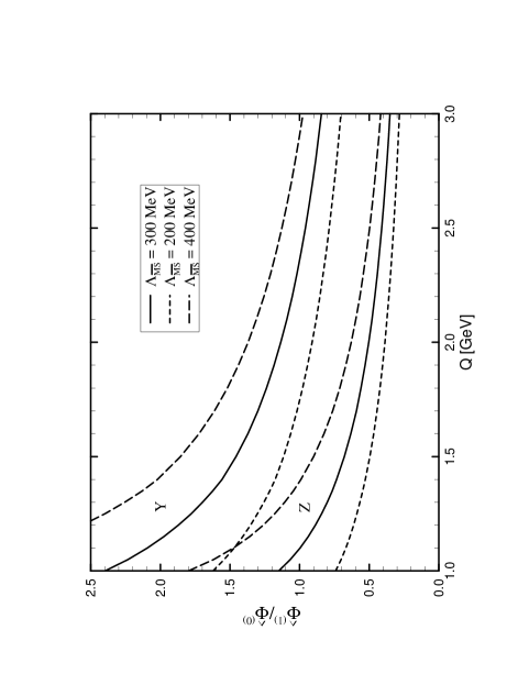
Figure 3: The ratios $\widehat{\Phi}^{(1)}_{z}/\widehat{\Phi}^{(0)}_{z}$ and $\widehat{\Phi}^{(1)}_{y}/\widehat{\Phi}^{(0)}_{y}$.

where the superscripts $(0)$ and $(1)$ refer to the leading as well as next-to-leading order respectively. In fig. 3, we plot the ratios $\widehat{\Phi}^{(1)}_{z}/\widehat{\Phi}^{(0)}_{z}$ and $\widehat{\Phi}^{(1)}_{y}/\widehat{\Phi}^{(0)}_{y}$ for $\Lambda_{\overline{MS}}=200,\,300$, and $400$ MeV. For simplicity, in fig. 3, we have not included the quark threshold at $m_{c}$, but we work in a theory with $f=3$ up to $3\,\mbox{\rm GeV}$. We have checked that these threshold effects only cause a small change in the NLO correction. Of course, as expected, the values for $\widehat{\Phi}_{z,\,y}$ in the HV and NDR scheme exactly agree.

From fig. 3, we can see that in the region $Q=1-3\,\mbox{\rm GeV}$, and for a central value $\Lambda_{\overline{MS}}=300\,\mbox{\rm MeV}$, the radiative QCD correction to $\widehat{\Phi}_{z}$ ranges approximately between 40% and 120%, whereas in the case of $\widehat{\Phi}_{y}$ we find a correction on the order of 100%–240%. Because the 2–point function is constructed as the square of the effective Hamiltonian, the actual corrections to ${\cal H}^{\Delta S=1}_{\mbox{\rm\scriptsize eff}}$ are only about half the corrections to the 2–point function. Therefore, the perturbative QCD correction to the real part of the effective Hamiltonian turns out to be 20%–60%, and for the imaginary part 50%–120%.

In sect. 3.3, we have demonstrated that the large $\alpha_{s}$ corrections correspond to the $\Delta I=1/2$ part of the effective weak Hamiltonian. The corrections to the $\Delta I=3/2$ part are identical to the ones in the $\Delta S=2$ correlator (both operators are in the same representation of the chiral group), which, as shown in sect. 3.3 and the next section, are quite moderate and negative. This implies that for the $\Delta I=1/2$–rule in $K\rightarrow\pi\pi$ decays, we receive an additional large and positive contribution, bringing theoretical calculations closer to the experimental value.

The calculation of the imaginary part of $\cal H_{\mbox{\rm\scriptsize eff}}$, no longer retains perturbative character, because of the large corrections. Nevertheless, this does not completely spoil existing determinations of weak matrix elements in the framework of the $1/N$ expansion or chiral perturbation theory, for there, to a given order in $1/N$ or the chiral expansion, the largest corrections in $\alpha_{s}$ are completely summed to all orders.

6 The $\Delta S=2$ operator

For the case of $\Delta S=2$ transitions, things are somewhat simpler because there is only one operator. We take this operator to be

$$Q_{\Delta S=2}\;\equiv\;\frac{1}{2}\,\Big{[}\,\left(\bar{s}d\right)_{\rm V-A}\left(\bar{s}d\right)_{\rm V-A}+\left(\bar{s}_{\alpha}d_{\beta}\right)_{\rm V-A}\left(\bar{s}_{\beta}d_{\alpha}\right)_{\rm V-A}\,\Big{]}\,.$$ (6.1)

This definition might seem unfamiliar, but we shall discuss in the following, why it is convenient. First, let us note that it renormalizes into itself, even in a general dimension, and it is obviously Fierz-symmetric. Apart from the quark content it has the same structure as $Q_{+}$.

Collecting the contributing diagrams, and making use of the relation (3.11), the 2–point function of $Q_{\Delta S=2}$ is given by

$$\Psi_{\Delta S=2}\;=\;\Psi_{11}+\Psi_{12}+\Psi_{13}+\Psi_{14}\,.$$ (6.2)

From this expression, we obtain the following values for $A$, $B$, and $X$:

$$A_{\Delta S=2} = \frac{8}{45}\,N\Big{(}N+1\Big{)}\,,$$ (6.3)

$$\vbox{\vskip 22.76219pt}B_{\Delta S=2}^{HV} = -\,\frac{3274}{1575}\,N\Big{(}N+1\Big{)}\,;\qquad B_{\Delta S=2}^{NDR}\;=\;-\,\frac{1246}{675}\,N\Big{(}N+1\Big{)}\,,$$ (6.4)

$$\vbox{\vskip 22.76219pt}X_{\Delta S=2}^{HV} = NC_{f}\,\biggl{(}\frac{4N}{15}-\frac{484}{225}\biggr{)}\,;\qquad X_{\Delta S=2}^{NDR}\;=\;NC_{f}\,\biggl{(}\frac{4N}{15}-\frac{188}{75}\biggr{)}\,.$$ (6.5)

As was already remarked at the end of the last section, up to a multiplicity factor 4, these quantities agree with the corresponding expressions for $\Psi_{++}$ of sect. 3.3, if we would refrain from performing the rotation of eq. (3.23) to a scheme-invariant basis. $C_{\Delta S=2}$ again respects eq. (2.10), and the relation between schemes (2.17) is also satisfied with

$$\Delta r_{\Delta S=2}\;=\;\frac{1}{2}\,\biggl{(}\,1-\frac{1}{N}\,\biggr{)}\,,$$ (6.6)

being easily obtained from ref. [8].

In the HV scheme, we could have worked with the operator

$$O_{\Delta S=2}\;\equiv\;\left(\bar{s}d\right)_{\rm V-A}\left(\bar{s}d\right)_{\rm V-A}\,,$$ (6.7)

in 4 dimensions being equivalent to $Q_{\Delta S=2}$, since in HV Fierz-symmetry is respected for current-current operators, and $O_{\Delta S=2}$ renormalizes into itself. This is not true for the NDR scheme and we would have to go through a similar procedure as described in sect. 3.2. Namely, augmenting the basis by an evanescent operator $E_{\Delta S=2}=\widetilde{O}_{\Delta S=2}-O_{\Delta S=2}$ and including this operator for renormalization, because it induces additional contributions to the physical subspace. We have checked that this treatment leads to the same value for $X^{NDR}_{\Delta S=2}$. Let us point out that this only concerns the quantities $B^{NDR}_{\Delta S=2}$ and $D^{NDR}_{\Delta S=2}$. The anomalous dimensions of $Q_{\Delta S=2}$ and $O_{\Delta S=2}$ in the NDR scheme agree even at NLO.

In order to be able to form the scheme-independent combination $\widehat{\Phi}_{\Delta S=2}(s)$, we need the Wilson-coefficient function for $\Delta S=2$ processes at NLO. It can be obtained from refs. [5, 6] for internal top and charm quark exchange in the box-diagram. The mixed charm-top contribution is not yet available at NLO. However, here we shall not pursue this any further, but use the strategy of ref. [5] of defining a scale- and scheme-invariant operator for $\Delta S=2$. This operator is given by

$$\widehat{Q}_{\Delta S=2}\;\equiv\;\alpha_{s}(\mu^{2})^{\gamma^{(1)}_{\Delta S=2}/\beta_{1}}\biggl{[}\,1-\frac{\alpha_{s}}{4\pi}\,Z\,\biggr{]}\,Q_{\Delta S=2}\,,$$ (6.8)

where $\gamma^{(1)}_{\Delta S=2}=\gamma^{(1)}_{+}$ is the LO anomalous dimension of $Q_{\Delta S=2}$. The finite NLO correction $Z$ depends on the scheme, and can be found in [5]. The matrix element of this operator is directly parametrized in terms of the scheme-invariant $B$-parameter $B_{K}$ for $K^{0}-\overline{K^{0}}$-mixing.

Calculating the spectral function $\widehat{\Phi}_{\Delta S=2}(s)$ for $\widehat{Q}_{\Delta S=2}$, we obtain

$$\widehat{\Phi}_{\Delta S=2}(s)\;=\;\theta(s)\,\frac{s^{4}}{(4\pi)^{6}}\,\alpha_{s}(s)^{2\gamma^{(1)}_{\Delta S=2}/\beta_{1}}\biggl{[}\,A_{\Delta S=2}+\frac{\alpha_{s}(s)}{\pi}\,\widehat{X}_{\Delta S=2}\,\biggr{]}\,,$$ (6.9)

with $\widehat{X}_{\Delta S=2}=4\,\widehat{X}_{+}$, and $\widehat{X}_{+}$ being given in eq. (3.29). This function is explicitly scheme-invariant, and for $N=3$ takes the form

$$\widehat{\Phi}_{\Delta S=2}(s)\;=\;\theta(s)\,\frac{32}{15}\,\frac{s^{4}}{(4\pi)^{6}}\,\alpha_{s}(s)^{-4/9}\biggl{[}\,1-\frac{3649}{1620}\,\frac{\alpha_{s}(s)}{\pi}\,\biggr{]}\,.$$ (6.10)

Because both, $Q_{+}$ and $Q_{\Delta S=2}$, have the same chiral representation, as expected, apart from a global factor, their spectral functions agree. We observe that the NLO QCD-correction is negative and on the order of 20%, for $\alpha_{s}(s)/\pi\approx 0.1$.

7 Discussion

Our work improves and completes the 2–point function evaluation of ref. [26] with two major additions: the recently calculated NLO corrections to the Wilson-coefficient functions have been taken into account and, moreover, we have incorporated the missing contributions from evanescent operators. The final results are then renormalization scheme- and scale-independent at the NLO, and, therefore, constitute the first complete calculation of weak non-leptonic observables at the NLO, without any hadronic ambiguity.

It is worthwhile to make a comparison with the results of ref. [26]. In this work, the NDR scheme was used and the calculation of the 2–point function for the $\Delta S=1$ case was performed in the basis

$$\widetilde{Q}\;=\;\Big{(}\,\widetilde{Q}_{1},\,Q_{2},\,Q_{3},\,\widetilde{Q}_{4},\,Q_{5},\,\widetilde{Q}_{6}\Big{)}\,,$$ (7.1)

not being plagued by problems with $\gamma_{5}$. The topologies present in that calculation were 1a, 1b, 2a, 2b, 2c, 2d, 2f, and 2g. We have reproduced the results for all these diagrams and we fully agree with ref. [26]. However, as already remarked in sects. 3 and 4, in the NDR scheme the basis (7.1) does not close under renormalization, and we had to add contributions from evanescent operators which were not included in [26]. In the notation of sect. 3, these evanescent contributions shift the matrices $\widetilde{B}^{NDR}$ and $\widetilde{D}^{NDR}$ to $B^{NDR}$ and $D^{NDR}$, and therefore the final correction $X^{NDR}$ gets changed. In addition, the relation $\widetilde{Q}_{4}=Q_{3}+Q_{2}-\widetilde{Q}_{1}$ for $f=3$ was used in ref. [26] to eliminate $\widetilde{Q}_{4}$. As it stands this relation is valid on the operator level.

Removing the entries for $Q_{4}$ from our matrices $B^{NDR}$, $D^{NDR}$, and $X^{NDR}$, and setting $f=3$, one can easily see the differences with the results of ref. [26]. The evanescent contributions have changed the entries (1,2), (1,3), and (6,6) of $B^{NDR}$, and (1,2) and (6,6) in $D^{NDR}$. The differences in $B^{NDR}$ propagate via the matrix products of eq. (2.9) into most entries of $X^{NDR}$: all entries except for (5,5) and the trivial zeros in (1,5), (2,5), and (3,5) are different. The final numerical differences are however not big, since the most sizeable $\alpha_{s}$ corrections were already included in the original calculation of ref. [26].

In the large-$N$ limit the operator $Q_{6}$ factorizes in the product of two current operators. Therefore, the 2–point function $\Psi_{66}$ can be calculated as a convolution of two current-correlators. This was used in [26] as a check for $\Psi_{66}$ at the leading order in $1/N$. In fact, the large-$N$ limit result of ref. [26] was already a full NLO calculation, since the corresponding anomalous dimension $\gamma_{66}$ was already known at the NLO (it is related to the quark-mass anomalous dimension in the large-$N$ limit) and it was correctly taken into account. Although our results for $B_{66}^{NDR}$ and $D_{66}^{NDR}$ show a discrepancy to the result of [26] even at the leading order in $1/N$, the combination $X_{66}^{NDR}$ only deviates from the result of [26] by subleading terms in the $1/N$-expansion, hence fulfilling the test in both cases. The differences at intermediate steps of the calculation ($B_{66}^{NDR}$ and $D_{66}^{NDR}$) stem from the fact that a different form of the operator ($Q_{6}$ or $\widetilde{Q}_{6}$) is being used, but the final physical result is of course identical.

For the $\Delta S=2$ operator the evanescent contributions result in changes in all next-to-leading quantities $B_{\Delta S=2}^{NDR}$, $D_{\Delta S=2}^{NDR}$, and $X_{\Delta S=2}^{NDR}$. The coefficient of the NLO correction to $\overline{\Phi}_{\Delta S=2}$, eq. (6.10), was found to be $-1217/810$ in ref. [26], compared to $-3649/1620$ in our case. This correction was used in ref. [25] for a sum rule determination of $B_{K}$. The effect of our new result would be to slightly further reduce the value of $B_{K}$ obtained in ref. [25].

Qualitatively, the conclusions of ref. [26] remain unchanged. At the NLO, the $\Delta I=1/2$ piece of the $\Delta S=1$ effective Hamiltonian gets a huge positive correction, while the gluonic effects in the $\Delta I=3/2$ (and $\Delta S=2$) operator are moderate and negative. Together with the previously known enhancement of the Wilson-coefficient [1, 2, 7, 4], this provides a very suggestive explanation of the observed enhancement of $\Delta I=1/2$ transitions in $K$ decays.

As explicitly shown in fig. 3, the NLO gluonic contributions are even more important in the CP-violating piece of the weak $\Delta S=1$ Hamiltonian; the reason being that this part is dominated by the penguin operator $Q_{6}$, which gets the largest correction. As shown in ref. [26], this enhancement is further reinforced at ${\cal O}(\alpha_{s}^{2})$, indicating a blow-up of the perturbative series in this case. Fortunately, this non-perturbative character does not completely prevent the feasibility of a reliable determination of CP-violating effects, since these leading contributions in $1/N$ can be resummed to all orders.

In a series of articles [34, 35, 36, 37] a more phenomenological description of the $\Delta I=1/2$–rule was advocated. The key idea is to rewrite the 4–quark operators as a product of diquark-anti-diquark operators by means of Fierz-transformations, and treating the diquark as an effective particle, similar to the constituent quarks. The important observation then lies in the dominance of pseudoscalar diquark matrix elements for low momentum transfer over axialvector meson matrix elements which are proportional to the momentum. All low energy decays in which diquarks can participate show the enhancement of $\Delta I=1/2$ amplitudes and a surprisingly good description of those processes was obtained.

An inspection of our results at the diagrammatic level reveals the following pattern for the origin of large corrections: all 2–point functions (except those which vanish at lowest order) receive contributions from the self-energy diagrams 2a or 2b, as well as from the quark-antiquark vertex corrections 2c, 2d, or 2e’. These contributions cancel to a fair amount:

$$C_{2\cdot 2a+2c}\;=\;C_{2\cdot 2a+2e^{\prime}}\;=\;C_{2\cdot 2b+2d} = 0\,,$$ (7.2)

$$\vbox{\vskip 22.76219pt}D^{NDR}_{2\cdot 2a+2c}\;=\;D^{NDR}_{2\cdot 2a+2e^{\prime}}\;=\;D^{NDR}_{2\cdot 2b+2d} = \frac{1}{15}\,,$$ (7.3)

$$\vbox{\vskip 22.76219pt}D^{HV}_{2\cdot 2a+2c}\;=\;D^{HV}_{2\cdot 2a+2e^{\prime}}\;=\;D^{HV}_{2\cdot 2b+2d} = \frac{7}{45}\,.$$ (7.4)

The quark-quark and antiquark-antiquark correlation diagrams 2e or 2f already by themselves are the biggest terms, and due to the partial cancellation of self-energy and current-vertex diagrams, we receive large corrections wherever quark-quark correlations can contribute. Note that these diagrams are subleading in $1/N$. The penguin diagrams 2g, 2g’, and 2g” generally have small impact on the 2-point functions.

This structure of the radiative corrections to 2–point functions of $\Delta S=1$ and $\Delta S=2$ operators allows for a deeper understanding, why the description of non-leptonic weak decays in terms of diquarks was so successful as far as the $\Delta I=1/2$–rule is concerned. In this framework, by working with effective diquarks, the quark-quark correlations were phenomenologically summed up to all orders in the strong coupling. Since these are the dominant corrections to the 2–point functions, summing them up provides us with a very good physical picture of the underlying QCD dynamics. As such, though, the statement in question, like the diquark-current itself, is gauge-dependent. In fact, the gauge-invariant combinations of diagrams are $(2\cdot 2a+2c)$, $(2\cdot 2a+2e^{\prime})$, $(2e+2e^{\prime})$, as well as their corresponding Fierz-conjugates. However, now the gauge-independent combination involving the quark-quark correlations dominates the other terms even more drastically (by one order of magnitude):

$$C_{2e+2e^{\prime}}\;=\;C_{2d+2f}\;=\;\frac{2}{15}\,,$$ (7.5)

$$D^{NDR}_{2e+2e^{\prime}}\;=\;-\,\frac{193}{90}\,,\qquad D^{NDR}_{2d+2f}\;=\;-\,\frac{181}{90}\,,$$ (7.6)

$$D^{HV}_{2e+2e^{\prime}}\;=\;D^{HV}_{2d+2f}\;=\;-\,\frac{1363}{630}\,.$$ (7.7)

A full QCD calculation has been possible because of the inclusive character of the defined 2–point functions. Although only qualitative conclusions can be directly extracted from these results, they are certainly important since they rigorously point to the QCD origin of the infamous $\Delta I=1/2$–rule, and, moreover, provide valuable information on the relative importance of the different operators, which can be very helpful to attempt more pragmatic calculations. Obviously, a direct application of our results would be the use of dispersion relations to extract “more exclusive” information from the 2–point functions, following the methods developed in refs. [20, 21, 22, 23, 24, 25, 26]. We plan to investigate this and other possible phenomenological applications in the future.

Acknowledgement

We would like to thank A. J. Buras and E. de Rafael for discussions and for reading the manuscript. M. J. would like to thank M. Neubert and P. H. Weisz for discussion. The Feynman diagrams were drawn with the aid of the program feynd, written by S. Herrlich. The work of A.P. has been supported in part by CICYT (Spain), under grant No. AEN93-0234.

Appendix

$$D^{NDR}=NC_{f}\!\left(\begin{array}[]{cccccc}\frac{2N}{15}&\frac{-187}{45}&\frac{2N}{15}&\frac{-35}{9}&0&0\\ \vbox{\vskip 17.07164pt}\frac{-187}{45}&\frac{2N}{15}-\frac{31}{81}&\frac{-377}{81}&\frac{2N}{15}-\frac{167f}{405}&0&\frac{-167f}{405}\\ \vbox{\vskip 17.07164pt}\frac{2N}{15}&\frac{-377}{81}&\frac{2fN}{15}-\frac{754}{81}&\frac{4N}{15}-\frac{2017f}{405}&0&\frac{-334f}{405}\\ \vbox{\vskip 17.07164pt}\frac{-35}{9}&\frac{2N}{15}-\frac{167f}{405}&\frac{4N}{15}-\frac{2017f}{405}&\frac{2fN}{15}-\frac{179f^{2}}{405}-\frac{70}{9}&0&\frac{-179f^{2}}{405}\\ \vbox{\vskip 17.07164pt}0&0&0&0&\frac{2fN}{15}&\frac{35f}{9}\\ \vbox{\vskip 17.07164pt}0&\frac{-167f}{405}&\frac{-334f}{405}&\frac{-179f^{2}}{405}&\frac{35f}{9}&\frac{187fN}{45}-\frac{179f^{2}}{405}\end{array}\right)$$

$$D^{HV}=NC_{f}\!\left(\begin{array}[]{cccccc}\frac{2N}{15}&\frac{-1321}{315}&\frac{2N}{15}&\frac{-1321}{315}&0&0\\ \vbox{\vskip 17.07164pt}\frac{-1321}{315}&\frac{2N}{15}-\frac{263}{567}&\frac{-14519}{2835}&\frac{2N}{15}-\frac{263f}{567}&\frac{4}{945}&\frac{-N}{105}-\frac{263f}{567}\\ \vbox{\vskip 17.07164pt}\frac{2N}{15}&\frac{-14519}{2835}&\frac{2fN}{15}-\frac{29038}{2835}&\frac{4N}{15}-\frac{14519f}{2835}&\frac{8}{945}&\frac{-2N}{105}-\frac{526f}{567}\\ \vbox{\vskip 17.07164pt}\frac{-1321}{315}&\frac{2N}{15}-\frac{263f}{567}&\frac{4N}{15}-\frac{14519f}{2835}&\frac{2fN}{15}-\frac{263f^{2}}{567}-\frac{2642}{315}&\frac{4f}{945}&\frac{-fN}{105}-\frac{263f^{2}}{567}\\ \vbox{\vskip 17.07164pt}0&\frac{4}{945}&\frac{8}{945}&\frac{4f}{945}&\frac{2fN}{15}-\frac{4}{105}&\frac{-2N}{105}+\frac{4387f}{945}\\ \vbox{\vskip 17.07164pt}0&\frac{-N}{105}-\frac{263f}{567}&\frac{-2N}{105}-\frac{526f}{567}&\frac{-fN}{105}-\frac{263f^{2}}{567}&\frac{-2N}{105}+\frac{4387f}{945}&\frac{1433fN}{315}-\frac{263f^{2}}{567}-\frac{4}{105}\end{array}\right)$$

Figures

Figure 1: Leading order diagrams for the 2–point function.

Figure 2: ${\cal O}(\alpha_{s})$ diagrams for the 2–point function.

References

[1]G. Altarelli, G. Curci, G. Martinelli, and S. Petrarca,
Nucl. Phys.B187 (1981) 461.
[2]A. J. Buras, M. Jamin, M. E. Lautenbacher, and P. H.
Weisz,
Nucl. Phys.B370 (1992) 69; add. ibid. B375 (1992)
501.
[3]M. Ciuchini, E. Franco, G. Martinelli, and L. Reina,
Phys. Lett.B301 (1993) 263.
[4]A. J. Buras, M. Jamin, and M. E. Lautenbacher,
Nucl. Phys.B408 (1993) 209.
[5]A. J. Buras, M. Jamin, and P. H. Weisz,
Nucl. Phys.B347 (1990) 491.
[6]S. Herrlich and U. Nierste,
Enhancement of the mass difference by short distance QCD
corrections beyond the leading order,
TU Munich preprint, TUM-T31-49/93, to appear in Nucl. Phys.B .
[7]A. J. Buras and P. H. Weisz,
Nucl. Phys.B333 (1990) 66.
[8]A. J. Buras, M. Jamin, M. E. Lautenbacher, and P. H.
Weisz,
Nucl. Phys.B400 (1993) 37.
[9]A. J. Buras, M. Jamin, and M. E. Lautenbacher,
Nucl. Phys.B400 (1993) 75.
[10]G. Curci and G. Ricciardi,
Phys. Rev.D47 (1993) 2991.
[11]M. Ciuchini, E. Franco, G. Martinelli, and L. Reina,
The Effective Hamiltonian Including Next-to-Leading
Order QCD and QED Corrections,
Rome preprint, 93/913, to appear in Nucl. Phys.B .
[12]R. Gupta, G. W. Kilcup, and S. R. Sharpe,
Nucl. Phys. B (Proc. Suppl.)26 (1992) 197.
[13]C. W. Bernard,
Heavy-light and light-light weak matrix elements on the lattice,
review presented at Lattice’93 (Dallas, 1993); and
references therein. .
[14]C. T. Sachrajda,
Lattice Phenomenology,
plenary talk at the EPS-93 Conference (Marseille 1993); and
references therein. .
[15]W. A. Bardeen, A. J. Buras, and J.-M. Gérard,
Nucl. Phys.B293 (1987) 787.
[16]W. A. Bardeen, A. J. Buras, and J.-M. Gérard,
Phys. Lett.B192 (1987) 138.
[17]W. A. Bardeen, A. J. Buras, and J.-M. Gérard,
Phys. Lett.B211 (1988) 343.
[18]J. Kambor, J. Missimer, and D. Wyler,
Phys. Lett.261B (1991) 496.
[19]J. Kambor, J. F. Donoghue, B. R. Holstein, J. Missimer,
and D. Wyler,
Phys. Rev. Lett.68 (1992) 1818.
[20]A. Pich and E. de Rafael,
Phys. Lett.158B (1985) 477.
[21]B. Guberina, A. Pich, and E. de Rafael,
Phys. Lett.163B (1985) 198.
[22]A. Pich, B. Guberina, and E. de Rafael,
Nucl. Phys.B277 (1986) 197.
[23]A. Pich and E. de Rafael,
Phys. Lett.B189 (1987) 369.
[24]A. Pich,
Nucl. Phys. B (Proc. Suppl.)7A (1989) 194.
[25]J. Prades, C. A. Dominguez, J. A. Peñarrocha, A. Pich, and E. de Rafael,
Z. Phys.C51 (1991) 287.
[26]A. Pich and E. de Rafael,
Nucl. Phys.B358 (1991) 311.
[27]G. ’t Hooft and M. Veltman,
Nucl. Phys.B44 (1972) 189.
[28]P. Breitenlohner and D. Maison,
Comm. Math. Phys.52 (1977) 11, 39, 55.
[29]M. K. Gaillard and B. W. Lee,
Phys. Rev. Lett.33 (1974) 108.
[30]G. Altarelli and L. Maiani,
Phys. Lett.52B (1974) 351.
[31]A. I. Vainshtein, V. I. Zakharov, and M. A. Shifman,
JEPT45 (1977) 670.
[32]F. J. Gilman and M. B. Wise,
Phys. Rev.D20 (1979) 2392.
[33]B. Guberina and R. D. Peccei,
Nucl. Phys.B163 (1980) 289.
[34]B. Stech,
Phys. Rev.D36 (1987) 975.
[35]H. G. Dosch, M. Jamin, and B. Stech,
Z. Phys.C42 (1989) 167.
[36]M. Neubert and B. Stech,
Phys. Lett.B231 (1989) 477.
[37]M. Neubert and B. Stech,
Phys. Rev.D44 (1991) 775.