(Published in “Progress in Particle and Nuclear Physics, 33 (1994) 201”.)

“The possibility that the universe was generated from nothing is very interesting and should be further studied. A most perplexing question relating to the singularity is this: what preceded the genesis of the universe? This question appears to be absolutely methaphysical, but our experience with metaphysics tells us that metaphysical questions are sometimes given answers by physics.”
A. Linde (1982)

Chapter 1 Introduction

The questions concerning the origin of our universe have long been thought of as metaphysical and hence outside the realm of physics.

However, tremendous advances in experimental techniques to study both the very large scale structures of the universe with space telescopes as well as the tiniest building blocks of matter – the quarks and leptons – with large accelerators, allow us “to put things together”, so that the creation of our universe now has become an area of active research in physics.

The two corner stones in this field are:

• Cosmology, i.e. the study of the large scale structure and the evolution of the universe. Today the central questions are being explored in the framework of the Big Bang Theory (BBT)[1, 2, 3, 4, 5], which provides a satisfactory explanation for the three basic observations about our universe: the Hubble expansion, the 2.7 K microwave background radiation, and the density of elements (74% hydrogen, 24% helium and the rest for the heavy elements).

• Elementary Particle Physics, i.e. the study of the building blocks of matter and the interactions between them. As far as we know, the building blocks of matter are pointlike particles, the quarks and leptons, which can be grouped according to certain symmetry principles; their interactions have been codified in the so-called Standard Model (SM)[6]. In this model all forces are described by gauge field theories[7], which form a marvelous synthesis of Symmetry Principles and Quantum Field Theories. The latter combine the classical field theories with the principles of Quantum Mechanics and Einstein’s Theory of Relativity.

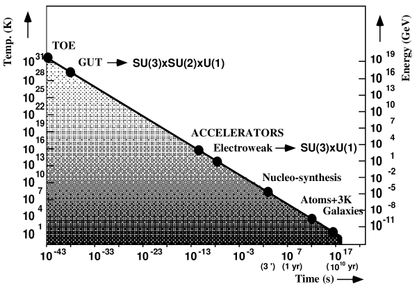
Figure 1.1: The evolution of the universe and the energy scale of some typical events: above the Planck scale of $10^{19}$   GeV gravity becomes so strong, that one cannot neglect gravity implying the need for a “Theory Of Everything” to describe all forces. Below that energy the well known strong and electroweak forces are assumed to be equally strong, implying the possibility of a Grand Unified Theory (GUT) with only a single coupling constant at the unification scale. After spontaneous symmetry breaking the gauge bosons of this unified force become heavy and ”freeze out”. The remaining forces correspond to the well known ${SU(3)_{C}\otimes\-SU(2)_{L}\otimes\-U(1)_{Y}}$  symmetry at lower energies with their coupling constants changing from the unified value at the GUT scale to the low energy values; this evolution is attributed to calculable radiative corrections. Future accelerators are expected to reach about 15 TeV corresponding to a temperature of $10^{15}$ K, which was reached about $10^{-12}$ s after the “Bang”. At about $10^{2}$  GeV the gauge bosons of the electroweak theory “freeze out” after getting mass through spontaneous symmetry breaking and only the strong and electromagnetic force play a role. About three minutes later the temperature has dropped below the nuclear binding energy and the strong force binds the quarks into nuclei (nucleosynthesis). Most of the particles annihilate with their antiparticles into a large number of photons after the photon energies become too low to create new particles again. After about hundred thousand years the temperature is below the electromagnetic binding energies of atoms, so the few remaining electrons and protons, which did not annihilate, form the neutral atoms. Then the universe becomes transparent for electromagnetic radiation and the many photons stream away into the universe. The photons released at that time are now observed as the 3 K microwave background radiation. Then the neutral atoms start to cluster slowly into stars and galaxies under the influence of gravity.

The basic observations, both in the Microcosm as well as in the Macrocosm, are well described by both models. Nevertheless, many questions remain unanswered. Among them:

• What is the origin of mass?

• What is the origin of matter?

• What is the origin of the Matter-Antimatter Asymmetry in our universe?

• Why is our universe so smooth and isotropic on a large scale?

• Why is the ratio of photons to baryons in the universe so extremely large, on the order of $10^{10}$?

• What is the origin of dark matter, which seems to provide the majority of mass in our universe?

• Why are the strong forces so strong and the electroweak forces so weak?

Grand Unified Theories (GUT)[8, 9], in which the known electromagnetic, weak, and strong nuclear forces are combined into a single theory, hold the promise of answering at least partially the questions raised above. For example, they explain the different strengths of the known forces by radiative corrections. At high energies all forces are equally strong. The Spontaneous Symmetry Breaking (SSB) of a single unified force into the electroweak and strong forces occurs in such theories through scalar fields, which “lock” their phases over macroscopic distances below the transition temperature. A classical analogy is the build-up of the magnetization in a ferromagnet below the Curie-temperature: above the transition temperature the phases of the magnetic dipoles are randomly distributed and the magnetization is zero, but below the transition temperature the phases are locked and the groundstate develops a nonzero magnetization. Translated in the jargon of particle physicists: the groundstate is called the vacuum and the scalar fields develop a nonzero “vacuum expectation value”. Such a phase transition might have released an enormous amount of energy, which would cause a rapid expansion (“inflation”) of the universe, thus explaining simultaneously the origin of matter, its isotropic distribution and the flatness of our universe.

Given the importance of the questions at stake, GUT’s have been under intense investigation during the last years.

The two directly testable predictions of the simplest GUT, namely

• the finite lifetime of the proton

• and the unification of the three coupling constants of the electroweak and strong forces at high energies

turned out to be a disaster for GUT’s. The proton was found to be much more stable than predicted and from the precisely measured coupling constants at the new electron-positron collider LEP at the European Laboratory for Elementary Particle Physics -CERN- in Geneva one had to conclude that the couplings did not unify, if extrapolated to high energies[10, 11, 12].

However, it was shown later, that by introducing a hitherto unobserved symmetry, called Supersymmetry (SUSY)[13, 14], into the Standard Model, both problems disappeared: unification was obtained and the prediction of the proton life time could be pushed above the present experimental lower limit!

The price to be paid for the introduction of SUSY is a doubling of the number of elementary particles, since it presupposes a symmetry between fermions and bosons, i.e. each particle with even (odd) spin has a partner with odd (even) spin. These supersymmetric partners have not been observed in nature, so the only way to save Supersymmetry is to assume that the predicted particles are too heavy to be produced by present accelerators. However, there are strong theoretical grounds to believe that they can not be extremely heavy and in the minimal SUSY model, the lightest so-called Higgs particle will be relatively light, which implies that it might even be detectable by upgrading the present LEP accelerator. But SUSY particles, if they exist, should be observable in the next generation of accelerators, since mass estimates from the unification of the precisely measured coupling constants are in the TeV region[11] and the lightest Higgs particle is expected to be of the order of ${M_{Z}}$, as will be discussed in the last chapter.

It is the purpose of the present paper to discuss the experimental tests of GUT’s. The following experimental constraints have been considered:

• Unification of the gauge coupling constants;

• Unification of the Yukawa couplings;

• Limits on proton decay;

• Electroweak breaking scale;

• Radiative $b\rightarrow s\gamma$ decays;

• Relic abundance of dark matter.

It is surprising that one can find solutions within the minimal SUSY model, which can describe all these independent results simultaneously. The constraints on the couplings, the unknown top-quark mass and the masses of the predicted SUSY particles will be discussed in detail.

The paper has been organized as follows: In chapters 2 to 4 the Standard Model, Grand Unified Theories (GUT) and Supersymmetry are introduced. In chapter 5 the problems in cosmology will be discussed and why cosmology “cries” for Supersymmetry. Finally, in chapter 6 the consistency checks of GUT’s through comparison with data are performed and in chapter 7 the results are summarized.

Chapter 2 The Standard Model.

2.1 Introduction.

The field of elementary particles has developed very rapidly during the last two decades, after the success of QED as a gauge field theory of the electromagnetic force could be extended to the weak– and strong forces. The success largely started with the November Revolution in 1974, when the charmed quark was discovered simultaneously at SLAC and Brookhaven, for which B. Richter and S.S.C Ting were awarded the Nobel prize in 1976. This discovery left little doubt that the pointlike constituents inside the proton and other hadrons are real, existing quarks and not some mathematical objects to classify the hadrons, as they were originally proposed by Gellman and independently by Zweig.

The existence of the charmed quark paved the way for a symmetry between quarks and leptons, since with charm one now had four quarks ($u,d,c$ and $s$) and four leptons ($e,\mu,\nu_{e}$ and $\nu_{\mu}$), which fitted nicely into the $SU(2)\otimes U(1)$ unified theory of the electroweak interactions proposed by Glashow, Salam and Weinberg (GSW) [6] for the leptonic sector and extended to include quarks as well as leptons by Glashow, Iliopoulis and Maiani (GIM) [16] as early as 1970. Actually, from the absence of flavour changing neutral currents, they predicted the charm quark with a mass around 1-3 GeV and indeed the charmed quark was found four years later with a mass of about 1.5 GeV. This discovery became known as the November Revolution, mentioned above.

The unification of the electromagnetic and weak interactions had already been forwarded by Schwinger and Glashow in the sixties. Weinberg and Salam solved the problem of the heavy gauge boson masses, required in order to explain the short range of the weak interactions, by introducing spontaneous symmetry breaking via the Higgs-mechanism. This introduced gauge boson masses without explicitly breaking the gauge symmetry.

The Glashow-Weinberg-Salam theory led to three important predictions:

• neutral currents, i.e. weak interactions without changing the electric charge. In contrast to the charged currents the neutral currents could occur with leptons from different generations in the initial state, e.g. $\nu_{\mu}e\rightarrow\nu_{\mu}e$ through the exchange of a new neutral gauge boson.

• the prediction of the heavy gauge boson masses around 90 GeV.

• a scalar neutral particle, the Higgs boson.

The first prediction was confirmed in 1973 by the observation of $\nu_{\mu}$ scattering without muon in the final state in the Gargamelle bubble chamber at CERN. Furthermore, the predicted parity violation for the neutral currents was observed in polarized electron-deuteron scattering and in optical effects in atoms. These successful experimental verifications[7] led to the award of the Nobel prize in 1979 to Glashow, Salam and Weinberg. In 1983 the second prediction was confirmed by the discovery of the $W$ and $Z$ bosons at CERN in $p\bar{p}$ collisions, for which C. Rubbia and S. van der Meer were awarded the Nobel prize in 1985.

The last prediction has not been confirmed: the Higgs boson is still at large despite intensive searches. It might just be too heavy to be produced with the present accelerators. No predictions for its mass exist within the Standard Model. In the supersymmetric extension of the SM the mass is predicted to be on the order of 100 GeV, which might be in reach after an upgrading of LEP to 210 GeV. These predictions will be discussed in detail in the last chapter, where a comparison with available data will be made.

In between the gauge theory of the strong interactions, as proposed by Fritzsch and Gell-Mann [17], had established itself firmly after the discovery of its gauge field, the gluon, in 3-jet production in ${e^{+}e^{-}}$ annihilation at the DESY laboratory in Hamburg. The colour charge of these gluons, which causes the gluon self-interaction, has been established firmly at CERN’s Large Electron Positron storage ring, called LEP. This gluon self-interaction leads to asymptotic freedom, as shown by Gross and Wilcek [18] and independently by Politzer [19], thus explaining why the quarks can be observed as almost free pointlike particles inside hadrons, and why they are not observed as free particles, i.e. they are confined inside these hadrons. This simultaneously explained the success of the Quark Parton Model, which assumes quasi-free partons inside the hadrons. In this case the cross sections, if expressed in dimensionless scaling variables, are independent of energy. The observation of scaling in deep inelastic lepton-nucleon scattering led to the award of the Nobel Prize to Freedman, Kendall and Taylor in 1990. Even the observation of logarithmic scaling violations, both in DIS and ${e^{+}e^{-}}$ annihilation, as predicted by QCD, were observed and could be used for precise determinations of the strong coupling constant of QCD[20, 21].

The discovery of the beauty quark at Fermilab in Batavia(USA) in 1976 and the $\tau$-lepton at SLAC, both in 1976, led to the discovery of the third generation of quarks and leptons, of which the expected top quark is still missing. Recent LEP data indicate that its mass is around 166 GeV[22], thus explaining why it has not yet been discovered at the present accelerators. The third generation had been introduced into the Standard Model long before by Kobayashi and Maskawa in order to be able to explain the observed CP violation in the kaon system within the Standard Model.

From the total decay width of the ${Z^{0}}$ bosons, as measured at LEP, one concludes that it couples to three different neutrinos with a mass below ${M_{Z}}/2\approx 45$ GeV. This strongly suggests that the number of generations of elementary particles is not infinite, but indeed three, since the neutrinos are massless in the Standard Model. The three generations have been summarized in table 2.1 together with the gauge fields, which are responsible for the low energy interactions.

The gluons are believed to be massless, since there is no reason to assume that the $SU(3)$ symmetry is broken, so one does not need Higgs fields associated with the low energy strong interactions. The apparent short range behaviour of the strong interactions is not due to the mass of the gauge bosons, but to the gluon self-interaction leading to confinement, as will be discussed in more detail afterwards.

This chapter has been organized as follows: after a short description of the SM, we discuss it shortcomings and unanswered questions. They form the motivation for extending the SM towards a Grand Unified Theory, in which the electroweak– and strong forces are unified into a new force with only a single coupling constant. The Grand Unified Theories will be discussed in the next chapter. Although such unification can only happen at extremely high energies – far above the range of present accelerators – it still has strong implications on low energy physics, which can be tested at present accelerators.

2.2 The Standard Model

Constructing a gauge theory requires the following steps to be taken:

• Choice of a symmetry group on the basis of the symmetry of the observed interactions.

• Requirement of local gauge invariance under transformations of the symmetry group.

• Choice of the Higgs sector to introduce spontaneous symmetry breaking, which allows the generation of masses without breaking explicitly gauge invariance. Massive gauge bosons are needed to obtain the short-range behaviour of the weak interactions. Adding ad-hoc mass terms, which are not gauge-invariant, leads to non-renormalizable field theories. In this case the infinities of the theory cannot be absorbed in the parameters and fields of the theory. With the Higgs mechanism the theory is indeed renormalizable, as was shown by G. ’t Hooft[23].

• Renormalization of the couplings and masses in the theory in order to relate the bare charges of the theory to known data. The Renormalization Group analysis leads to the concept of “running”, i.e. energy dependent coupling constants, which allows the absorption of infinities in the theory into the coupling constants.

	Interactions
	strong	electro-weak	gravitational	unified ?
Theory	QCD	GSW	quantum gravity ?	SUGRA ?
Symmetry	$SU(3)$	$SU(2)\times U(1)$	?	SU(5)?
Gauge	$g_{1}\cdots g_{8}$	photon	G	X,Y ?
bosons	gluons	$W^{\pm}$  ,$Z^{0}$  bosons	graviton	GUT bosons?
charge	colour	weak isospin	mass	?
		weak hypercharge

Table 2.1: The fundamental forces. The question marks indicate areas of intensive research.

2.2.1 Choice of the Group Structure.

Groups of particles observed in nature show very similar properties, thus suggesting the existence of symmetries. For example, the quarks come in three colours, while the weak interactions suggest the grouping of fermions into doublets. This leads naturally to the $SU(3)$ and $SU(2)$ group structure for the strong and weak interactions, respectively. The electromagnetic interactions don’t change the quantum numbers of the interacting particles, so the simple $U(1)$ group is sufficient.

Consequently, the Standard Model of the strong and electroweak interactions is based on the symmetry of the following unitary groups:

$${SU(3)_{C}\otimes\-SU(2)_{L}\otimes\-U(1)_{Y}}.$$ (2.1)

The need for three colours arose in connection with the existence of hadrons consisting of three quarks with identical quantum numbers. According to the Pauli principle fermions are not allowed to be in the same state, so labeling them with different colours solved the problem[7]. More direct experimental evidence for colour came from the decay width of the $\pi^{0}$ and the total hadronic cross section in ${e^{+}e^{-}}$ annihilation[7]. Both are proportional to the number of quark species and both require the number of colours to be three.

Although colour was introduced first as an ad-hoc quantum number for the reasons given above, it became later evident, that its role was much more fundamental, namely that it acted as the source of the field for the strong interactions (the “colour” field), just like the electric charge is the source of the electric field.

The “charge” of the weak interactions is the third component of the “weak” isospin $T_{3}$. The charged weak interactions only operate on left-handed particles, i.e. particles with the spin aligned opposite to their momentum (negative helicity), so only left-handed particles are given weak isospin $\pm$ 1/2 and right-handed particles are put into singlets (see table 2.2). Right-handed neutrinos do not exist in nature, so within each generation one has 15 matter fields: 2(1) left(right)-handed leptons and 2x3 (2x3) left(right)-handed quarks (factor 3 for colour).

The electromagnetic interactions originate both from the exchange of the neutral gauge boson of the $SU(2)$ group as well as the one from the $U(1)$ group. Consequently the “charge” of the $U(1)$ group cannot be identical with the electric charge, but it is the so-called weak hypercharge -$Y_{W}$-, which is related to the electric charge via the Gell-Mann-Nishijima relation:

$$Q=T_{3}+\frac{1}{2}Y_{W}.$$ (2.2)

The quantum number $Y_{W}$ is $(B-L)$ for left handed doublets and $2Q$ for righthanded singlets, where the baryon number $B$=1/3 for quarks and 0 for leptons, while the lepton number $L$ =1 for leptons and 0 for quarks. Since $T_{3}$ and $Q$ are conserved, $Y_{W}$ is also a conserved quantum number. The electro-weak quantum numbers for the elementary particle spectrum are summarized in table 2.2.

	Generations			Quantum Numbers
helicity	1.	2.	3.	Q	$T_{3}$	$Y_{W}$
	$\left(\begin{array}[]{c}\nu_{e}\\ e\end{array}\right)_{L}$	$\left(\begin{array}[]{c}\nu_{\mu}\\ \mu\end{array}\right)_{L}$	$\left(\begin{array}[]{c}\nu_{\tau}\\ \tau\end{array}\right)_{L}$	$\begin{array}[]{r}0\\ -1\end{array}$	$\begin{array}[]{r}1/2\\ -1/2\end{array}$	$\begin{array}[]{r}-1\\ -1\end{array}$
L
	$\left(\begin{array}[]{c}u\\ d^{\prime}\end{array}\right)_{L}$	$\left(\begin{array}[]{c}c\\ s^{\prime}\end{array}\right)_{L}$	$\left(\begin{array}[]{c}t\\ b^{\prime}\end{array}\right)_{L}$	$\begin{array}[]{r}2/3\\ -1/3\end{array}$	$\begin{array}[]{r}1/2\\ -1/2\end{array}$	$\begin{array}[]{r}1/3\\ 1/3\end{array}$
	$e_{R}$	$\mu_{R}$	$\tau_{R}$	-1	0	-2
$\begin{array}[]{c}R\\ \end{array}$	$\begin{array}[]{c}u_{R}\\ d_{R}\end{array}$	$\begin{array}[]{c}c_{R}\\ s_{R}\end{array}$	$\begin{array}[]{c}t_{R}\\ b_{R}\end{array}$	$\begin{array}[]{r}2/3\\ -1/3\end{array}$	$\begin{array}[]{r}0\\ 0\end{array}$	$\begin{array}[]{r}4/3\\ -2/3\end{array}$

Table 2.2: The electro-weak quantum numbers (electric charge $Q$, third component of weak isospin $T_{3}$ and weak hypercharge $Y_{W}$) of the particle spectrum. The neutrinos $\nu_{e}$, $\nu_{\mu}$ and $\nu_{\tau}$ are the weak isospin partners of the electron($e$), muon($\mu$) and tau($\tau$) leptons, respectively. The up($u$), down($d$), strange($s$), charm($c$), bottom($b$) and top($t$) quarks come in three colours, which have not been indicated. The primes for the left handed quarks $d^{\prime}$, $s^{\prime}$ and $b^{\prime}$ indicate the interaction eigenstates of the electro-weak theory, which are mixtures of the mass eigenstates, i.e. the real particles. The mixing matrix is the Cabibbo-Kobayshi-Maskawa matrix. The weak hypercharge $Y_{W}$ equals $B-L$ for the left-handed doublets and $2Q$ for the right-handed singlets.

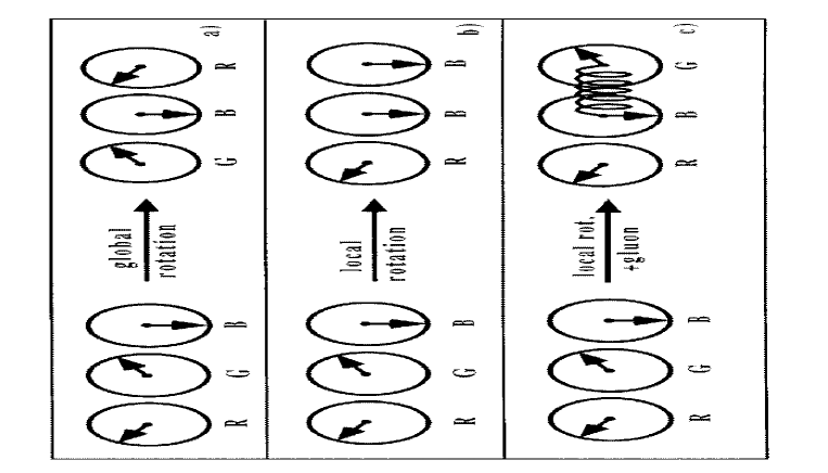
Figure 2.1: Global rotations leave the baryon colourless (a). Local rotations change the colour locally, thus changing the colour of the baryon (b), unless the colour is restored by the exchange of a gluon (c).

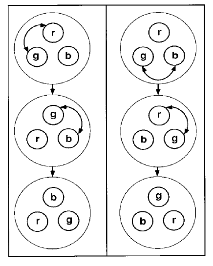
Figure 2.2: Demonstration of the non-abelian character of the SU(3) rotations inside a colourless baryon: on the left-hand side one first exchanges a red-green gluon, which exchanges the colours of the quarks, and then a green-blue gluon; on the right-hand side the order is reversed. The final result is not the same, so these operations do not commute.

2.3 Requirement of local gauge invariance.

The Lagrangian ${{\cal L}}$ of a free fermion can be written as:

$${{\cal L}}=i\overline{\Psi}\gamma^{\mu}\partial_{\mu}\Psi-m\overline{\Psi}\Psi,$$ (2.3)

where the first term represents the kinetic energy of the matter field $\Psi$ with mass $m$ and the second term is the energy corresponding to the mass $m$. The Euler-Lagrange equations for this ${{\cal L}}$ yield the Dirac equation for a free fermion.

The unitary groups $SU(N)$ introduced above represent rotations in $N$ dimensional space. The bases for the space are provided by the eigenstates of the matter fields, which are the colour triplets in case of $SU(3)$, weak isospin doublets in case of $SU(2)$ and singlets for $U(1)$.

Arbitrary rotations of the states can be represented by

$$U=exp(-i\vec{\alpha}\cdot\vec{F})=exp(-i\sum_{k=1}^{N^{2}-1}\alpha_{k}\cdot F_{k})$$ (2.4)

where $\alpha_{k}$ are the rotation parameters and $F_{k}$ the rotation matrices. $F_{k}$ are the eight 3x3 Gell-Mann matrices for $SU(3)$, denoted by $\lambda$ hereafter, and the well known Pauli matrices for $SU(2)$ denoted by $\tau$.

The Lagrangian is invariant under the $SU(N)$ rotation, if ${{\cal L}}(\Psi^{\prime})$ =${{\cal L}}(\Psi)$, where $\Psi^{\prime}=U\Psi$. The mass term is clearly invariant: $m\overline{\Psi}^{\prime}\Psi^{\prime}=m\overline{\Psi}U^{{\dagger}}U\Psi=m\overline{\Psi}\Psi$, since $U^{{\dagger}}U=1$ for unitary matrices. The kinetic term is only invariant under global transformations, i.e. transformations where $\alpha_{k}$ is everywhere the same in space-time. In this case $U$ is independent of $x$ and can be treated as a constant multiplying $\Psi$, which leads to: $\overline{\Psi}U^{{\dagger}}\gamma^{\mu}\partial_{\mu}U\Psi=\overline{\Psi}U^{{\dagger}}U\gamma^{\mu}\partial_{\mu}\Psi=\overline{\Psi}\gamma^{\mu}\partial_{\mu}\Psi$.

However, one could also require $\it local$ instead of global gauge invariance, implying that the interactions should be invariant under rotations of the symmetry group for each particle separately. The motivation is simply that the interactions should be the same for particles belonging to the same multiplet of a symmetry group. For example, the interaction between a green and a blue quark should be the same as the interaction between a green and a red quark; therefore it should be allowed to perform a local colour transformation of a single quark. The consequence of requiring local gauge invariance is dramatic: it requires the introduction of intermediate gauge bosons whose quantum numbers completely determine the possible interactions between the matter fields, as was first shown by Yang and Mills in 1957 for the isopin symmetry of the strong interactions.

Intuitively this is quite clear. Consider a hadron consisting of a colour triplet of quarks in a colourless groundstate. A global rotation of all quark fields will leave the groundstate invariant, as shown schematically in fig. 2.1. However, if a quark field is rotated locally, the groundstate is not colourless anymore, unless a “message” is mediated to the other quarks to change their colours as well. The “mediators” in $SU(3)$ are the gluons, which carry a colour charge themselves and the local colour variation of the quark field is restored by the gluons.

The colour charge of the gluons is a consequence of the non-abelian character of SU(3), which implies that rotations in colour space do not commute, i.e. $\lambda_{a}\lambda_{b}\neq\lambda_{b}\lambda_{a}$, as demonstrated in fig. 2.2. If the gluons would all be colourless, they would not change the colour of the quarks and their exchange would be commuting.

Mathematically, local gauge invariance is introduced by replacing the derivative $\partial_{\mu}$ with the covariant derivative $D_{\mu}$, which is required to have the following property:

$$D^{\prime}\Psi^{\prime}=UD\Psi,$$ (2.5)

i.e. the covariant derivative of the field has the same transformation properties as the field in contrast to the normal derivative. Clearly with this requirement ${{\cal L}}$ is manifestly gauge invariant, since in each term of eq. 2.3 the transformation leads to the product $U^{{\dagger}}U=1$ after substituting $\partial_{\mu}\rightarrow D_{\mu}.$

For infinitesimal transformations the covariant derivative can be written as[7]:

$$D_{\mu}=\partial_{\mu}+\frac{ig^{\prime}}{2}B_{\mu}{Y_{W}}+\frac{ig}{2}{\bf\vec{W}_{\mu}}\cdot{\bf\vec{\tau}}+\frac{ig_{s}}{2}{\bf\vec{G}_{\mu}}\cdot{\bf\vec{\lambda}},$$ (2.6)

where $B_{\mu},\bf\vec{W}_{\mu}$ and $\bf\vec{G}_{\mu}$ are the field quanta (“mediators”) of the $U(1)$, $SU(2)$ and $SU(3)$ groups and $g^{\prime},~{}g$ and $g_{s}$ the corresponding coupling constants.

The term ${\bf\vec{W}_{\mu}}\cdot{\bf\vec{\tau}}$ can be explicitly written as:

$$W^{1}_{\mu}\tau_{1}+W^{2}_{\mu}\tau_{2}+W^{3}_{\mu}\tau_{3}=W^{1}_{\mu}\left(\begin{array}[]{cc}0&1\\ 1&0\end{array}\right)+W^{2}_{\mu}\left(\begin{array}[]{cc}0&-i\\ i&0\end{array}\right)+W^{3}_{\mu}\left(\begin{array}[]{cc}1&0\\ 0&-1\end{array}\right)=$$

$$\left(\begin{array}[]{cc}W_{\mu}^{3}&W_{\mu}^{1}-iW_{\mu}^{2}\\ W_{\mu}^{1}+iW_{\mu}^{2}&-W_{\mu}^{3}\end{array}\right)\equiv\left(\begin{array}[]{cc}W_{\mu}^{3}&\sqrt{2}W^{+}\\ \sqrt{2}W^{-}&-W_{\mu}^{3}\end{array}\right)$$ (2.7)

The operators $W^{\pm}$ in the off-diagonal elements act as lowering- and raising operators for the weak isospin. For example, they transform an electron into a neutrino and vice-versa, while the operator $W_{\mu}^{3}$ represents the neutral current interactions between a fermion and antifermion.

After substituting the Gell-Mann matrices $\lambda$ the term ${\bf G_{\mu}\cdot\lambda}={\textstyle\sum_{k=1}^{8}}G_{k}\lambda_{k}$ can be written similarly as:

$$\left(\begin{array}[]{ccc}G_{\mu}^{3}+\frac{1}{\sqrt{3}}G^{8}&G^{1}-iG^{2}&G^{4}-iG^{5}\\ \\ G_{\mu}^{1}+iG^{2}&-G^{3}+\frac{1}{\sqrt{3}}G^{8}&G^{6}-iG^{7}\\ \\ G_{\mu}^{4}+iG^{5}&G^{6}+iG^{7}&-\frac{2}{\sqrt{3}}G^{8}\end{array}\right)\equiv\left(\begin{array}[]{ccc}G_{\mu}^{3}+\frac{1}{\sqrt{3}}G^{8}&\sqrt{2}G_{rg}&\sqrt{2}G_{rb}\\ \\ \sqrt{2}G_{gr}&-G^{3}+\frac{1}{\sqrt{3}}G^{8}&\sqrt{2}G_{gb}\\ \\ \sqrt{2}G_{br}&\sqrt{2}G_{bg}&-\frac{2}{\sqrt{3}}G^{8}\end{array}\right)$$

This term induces transitions between the colours. For example, the off-diagonal element $G_{rg}$ acts like a raising operator between a green $\Phi_{g}=(0,1,0)$ and red $\Phi_{r}=(1,0,0)$ field. The terms on the diagonal don’t change the colour. Since the trace of the matrix has to be zero, there are only two independent gluons, which don’t change the colour. They are linear combinations of the diagonal matrices $\lambda_{3}$ and $\lambda_{8}$.

The $W_{\mu}$ gauge fields cannot represent the mediators of the weak interactions, since the latter have to be massive. Mass terms for $W_{\mu}$, such as $M^{2}W_{\mu}W^{\mu}$, are not gauge invariant, as can be checked from the transformation laws for the fields. The real fields $\gamma,Z^{0},$ and $W^{\pm}$ can be obtained from the gauge fields after spontaneous symmetry breaking via the Higgs mechanism, as will be discussed in the next section.

2.4 The Higgs mechanism.

2.4.1 Introduction.

The problem of mass for the fermions and weak gauge bosons can be solved by assuming that masses are generated dynamically through the interaction with a scalar field, which is assumed to be present everywhere in the vacuum, i.e. the space-time in which interactions take place.

The vacuum or equivalently the groundstate, i.e. the state with the lowest potential energy, may have a non-zero (scalar) field value represented by $\Phi=v~{}exp(i\phi)$; $v$ is called the vacuum expectation value (vev). The same minimum is reached for an arbitrary value of the phase $\phi$, so there exists an infinity of different, but equivalent groundstates. This degeneracy of the ground state takes on a special significance in a quantum field theory, because the vacuum is required to be unique, so the phase cannot be arbitrarily at each point in space-time. Once a particular value of the phase is chosen, it has to remain the same everywhere, i.e. it cannot change locally. A scalar field with a nonzero vev therefore breaks local gauge invariance. More details can be found in the nice introduction by Moriyasu[7].

Nature has many examples of broken symmetries. Superconductivity is a well known example. Below the critical temperature the electrons bind into Cooper pairs. The density of Cooper pairs corresponds to the vev. Owing to the weak binding, the effective size of a Cooper pair is large, about $10^{-4}$ cm, so every Cooper pair overlaps with about $10^{6}$ other Cooper pairs and this overlap “locks” the phases of the wave function over macroscopic distances: “Superconductivity is a remarkable manifestation of Quantum Mechanics on a truly macroscopic scale” [24].

In the superconducting phase the photon gets an effective mass through the interaction with the Cooper pairs in the “vacuum”, which is apparent in the Meissner effect: the magnetic field has a very short penetration depth into the superconductor or equivalently the photon is very massive. Before the phase transition the vacuum would have zero Cooper pairs, i.e. a zero vev, and the magnetic field can penetrate the superconductor without attenuation as expected for massless photons.

This example of Quantum Mechanics and spontaneous symmetry breaking in superconductivity has been transferred almost literally to elementary particle physics by Higgs and others[25].

Figure 2.3: Shape of the Higgs potential for $\mu^{2}>0$ (a) and $\mu^{2}<0$ (b); $\phi_{1}$ and $\phi_{2}$ are the real and imaginary parts of the Higgs field.

For the self-interaction of the Higgs field one considers a potential analogous to the one proposed by Ginzburg and Landau for superconductivity:

$$V(\Phi)=\mu^{2}\;\Phi^{\dagger}\Phi+\lambda(\Phi^{\dagger}\Phi)^{2}$$ (2.8)

where $\mu^{2}$ and $\lambda$ are constants. The potential has a parabolic shape, if $\mu^{2}>0$, but takes the shape of a Mexican hat for $\mu^{2}<0$, as pictured in fig. 2.3. In the latter case the field free vacuum, i.e. $\Phi=0$, corresponds to a local maximum, thus forming an unstable equilibrium. The groundstate corresponds to a minimum with a nonzero value for the field:

$$|\Phi|=\sqrt{\frac{-\mu^{2}}{2\lambda}}.$$ (2.9)

In superconductivity $\mu^{2}$ acts like the critical temperature $T_{c}$: above $T_{c}$ the electrons are free particles, so their phases can be rotated arbitrarily at all points in space, but below $T_{c}$ the individual rotational freedom is lost, because the electrons form a coherent system, in which all phases are locked to a certain value. This corresponds to a single point in the minimum of the Mexican hat, which represents a vacuum with a nonzero vev and a well defined phase, thus defining a unique vacuum. The coherent system can still be rotated as a whole so it is invariant under global but not under local rotations.

2.4.2 Gauge Boson Masses and the Top Quark Mass.

After this general introduction about the Higgs mechanism, one has to consider the number of Higgs fields needed to break the $SU(2)_{L}\otimes U(1)_{Y}$ symmetry to the $U(1)_{em}$ symmetry. The latter must have one massless gauge boson, while the $W$ and $Z$ bosons must be massive. This can be achieved by choosing $\Phi$ to be a complex $SU(2)$ doublet with definite hypercharge ($Y_{W}=1$):

$$\Phi(x)=\left(\begin{array}[]{cc}\phi_{1}^{+}(x)&+i\phi^{+}_{2}(x)\\ \phi^{0}_{1}(x)&+i\phi^{0}_{2}(x)\end{array}\right)$$ (2.10)

In order to understand the interactions of the Higgs field with other particles, one considers the following Lagrangian for a scalar field:

$${{\cal L}}_{H}=(D_{\mu}\Phi)^{{\dagger}}(D^{\mu}\Phi)-V(\Phi).$$ (2.11)

The first term is the usual kinetic energy term for a scalar particle, for which the Euler-Lagrange equations lead to the Klein-Gordon equation of motion. Instead of the normal derivative, the covariant derivative is used in eq. 2.11 in order to ensure local gauge invariance under $SU(2)\otimes U(1)$ rotations.

The vacuum is known to be neutral. Therefore the groundstate of $\Phi$ has to be of the form (0,v). Furthermore $\Phi(x)$ has to be constant everywhere in order to have zero kinetic energy, i.e. the derivative term in ${{\cal L}}_{H}$ disappears.

The quantum fluctuations of the field around the ground state can be parametrised as follows, if we include an arbitrary $SU(2)$ phase factor:

$$\Phi=e^{i\vec{\zeta}(x)\cdot\vec{\tau}}\left(\begin{array}[]{c}0\\ v+h(x)\end{array}\right).$$ (2.12)

The (real) fields $\zeta(x)$ are excitations of the field along the potential minimum. They correspond to the massless Goldstone bosons of a global symmetry, in this case three for the three rotations of the $SU(2)$ group. However, in a local gauge theory these massless bosons can be eliminated by a suitable rotation:

$$\Phi^{\prime}=e^{-i\vec{\zeta}(x)\cdot\vec{\tau}}\Phi(x)=\left(\begin{array}[]{c}0\\ v+h(x)\end{array}\right).$$ (2.13)

Consequently the field $\zeta$ has no physical significance. Only the real field $h(x)$ can be interpreted as a real (Higgs) particle. The original field $\bf\Phi$ with four degrees of freedom has lost three degrees of freedom; these are recovered as the longitudinal polarizations of the three heavy gauge bosons.

The kinetic part of eq. 2.11 gives rise to mass terms for the vector bosons, which can be written as ($Y_{W}=1)$:

$${{\cal L}}_{H}=\frac{1}{4}\left[\left({g}(W_{\mu}^{1}\tau_{1}+W_{\mu}^{2}\tau_{2}+W_{\mu}^{3}\tau_{3})+g^{\prime}B_{\mu}\right)\Phi\right]^{{\dagger}}\left[\left({g}(W^{\mu 1}\tau_{1}+W^{\mu 2}\tau_{2}+W^{\mu 3}\tau_{3})+g^{\prime}B^{\mu}\right)\Phi\right]$$ (2.14)

or substituting for $\Phi$ its vacuum expectation value $v$ one obtains from the off-diagonal terms (by writing the $\tau$ matrices explicitly, see eq. 2.7)

$$\left(\frac{gv}{2}\right)^{2}\left((W_{\mu}^{1})^{2}+(W_{\mu}^{2})^{2}\right)$$ (2.15)

and from the diagonal terms:

$$\frac{1}{2}\left(\frac{v^{2}}{2}\right)\left(-gW_{\mu}^{3{\dagger}}+g^{\prime}B_{\mu}^{{\dagger}}\right)\left(-gW^{3\mu}+g^{\prime}B^{\mu}\right)=\\ \frac{1}{2}\left(\frac{v^{2}}{2}\right)\left(B_{\mu}^{{\dagger}}W_{\mu}^{3{\dagger}}\right)\left(\begin{array}[]{cc}+g^{\prime 2}&-gg^{\prime}\\ -gg^{\prime}&g^{2}\end{array}\right)\left(\begin{array}[]{c}B^{\mu}\\ W^{3\mu}\end{array}\right).$$

Since mass terms of physical fields have to be diagonal, one obtains the “physical” gauge fields of the broken symmetry by diagonalizing the mass term:

$$\left(B_{\mu}^{{\dagger}}W_{\mu}^{3{\dagger}}\right)~{}U^{-1}U~{}M~{}U^{-1}U~{}\left(\begin{array}[]{c}B^{\mu}\\ W^{3\mu}\end{array}\right)$$ (2.16)

where $U$ represents a unitary matrix

$$U=\frac{1}{\sqrt{g^{\prime 2}+g^{2}}}\left(\begin{array}[]{cc}g&g^{\prime}\\ -g^{\prime}&g\end{array}\right)\equiv\left(\begin{array}[]{cc}{\;\cos\theta_{W}}&{\;\sin\theta_{W}}\\ -{\;\sin\theta_{W}}&{\;\cos\theta_{W}}\end{array}\right)$$ (2.17)

Consequently the real fields become a mixture of the gauge fields:

$$\left(\begin{array}[]{c}A^{\mu}\\ Z^{\mu}\end{array}\right)~{}=~{}U~{}\left(\begin{array}[]{c}B^{\mu}\\ W^{3\mu}\end{array}\right)$$ (2.18)

and the matrix $UMU^{-1}$ becomes a diagonal matrix for a suitable mixing angle $\theta_{W}$.

In these fields the mass terms have the form

$$M_{W}^{2}W_{\mu}^{+}W^{-\mu}+\frac{1}{2}(A_{\mu},Z_{\mu})\left(\begin{array}[]{cc}0&0\\ 0&M_{Z}^{2}\end{array}\right)\left(\begin{array}[]{c}A^{\mu}\\ Z^{\mu}\end{array}\right)$$ (2.19)

with

$$M_{W}^{2}=\frac{1}{2}g^{2}v^{2}$$ (2.20)

$$M_{Z}^{2}=\frac{g^{\prime\;2}+g^{2}}{2}v^{2}.$$ (2.21)

Here $v$ is the vacuum expectation value of the Higgs potential, which for the known gauge boson masses and couplings can be calculated to be:

$$v\approx 174~{}{\rm GeV}.$$ (2.22)

The neutral part of the Lagrangian, if expressed in terms of the physical fields, can be written as:

$${{\cal L}}_{int}^{neutr} = -A_{\mu}[g^{\prime}\;{\;\cos\theta_{W}}(\overline{e}_{R}\gamma^{\mu}e_{R}+\frac{1}{2}\overline{\nu}_{L}\gamma^{\mu}\nu_{L}+\frac{1}{2}\overline{e}_{L}\gamma^{\mu}e_{L})-\frac{1}{2}g\;{\;\sin\theta_{W}}(\overline{\nu}_{L}\gamma^{\mu}\nu_{L}-\overline{e}_{L}\gamma^{\mu}e_{L})]$$

$$+Z_{\mu}[g^{\prime}{\;\sin\theta_{W}}(\overline{e}_{R}\gamma^{\mu}e_{R}+\frac{1}{2}\overline{\nu}_{L}\gamma^{\mu}\nu_{L}+\frac{1}{2}\overline{e}_{L}\gamma^{\mu}e_{L})+\frac{1}{2}g{\;\cos\theta_{W}}(\overline{\nu}_{L}\gamma^{\mu}\nu_{L}-\overline{e}_{L}\gamma^{\mu}e_{L})]$$

The photon field should only couple to the electron fields and not to the neutrinos, so the terms proportional to $g^{\prime}{\;\cos\theta_{W}}$ and $g{\;\sin\theta_{W}}$ should cancel and the coupling to the electrons has to be the electric charge $e$. This can be achieved by requiring:

$$g^{\prime}{\;\cos\theta_{W}}=g\;{\;\sin\theta_{W}}=e~{}.$$ (2.24)

Hence

$${\;\tan\theta_{W}}=\frac{g^{\prime}}{g}~{}~{};{\;\sin^{2}\theta_{W}}=\frac{g^{\prime 2}}{g^{2}+g^{\prime 2}}~{}~{}{\rm and}~{}~{}e=\frac{gg^{\prime}}{\sqrt{g^{2}+g^{\prime 2}}}.$$ (2.25)

Figure 2.4: Geometric picture of the relations between the electroweak coupling constants.

A geometric picture of these relations is shown in fig. 2.4. From these relations and the relations between masses and couplings (2.20 and 2.21) one finds the famous relation between the electroweak mixing angle and the gauge boson masses:

$$M_{W}={\;\cos\theta_{W}}\cdot M_{Z}\;\;\;{\rm or}~{}~{}~{}{\;\sin^{2}\theta_{W}}=1-\frac{M^{2}_{W}}{M^{2}_{Z}}\;.$$ (2.26)

The value of $M_{W}$ can also be related to the precisely measured muon decay constant $G_{\mu}=1.16639(2)\cdot 10^{-5}$ GeV^-2. If calculated in the SM, one finds:

$$\frac{G_{\mu}}{\sqrt{2}}=\frac{e^{2}}{8{\;\sin^{2}\theta_{W}}M_{W}^{2}}.$$ (2.27)

This relation can be used to calculate the gauge boson masses from measured coupling constants $\alpha$, $G_{\mu}$ and ${\;\sin\theta_{W}}$:

$$M_{W}^{2} = \frac{\pi\alpha}{\sqrt{2}G_{\mu}}\cdot\frac{1}{{\;\sin^{2}\theta_{W}}}$$ (2.28)

$$M_{Z}^{2} = \frac{\pi\alpha}{\sqrt{2}G_{\mu}}\cdot\frac{1}{{\;\sin^{2}\theta_{W}}{\;\cos^{2}\theta_{W}}}$$ (2.29)

Inserting ${\;\sin^{2}\theta_{W}}=0.23$ and $1/\alpha=137.036$ yields ${M_{Z}}$=88 GeV. However, these relations are only at tree level. Radiative corrections depend on the as yet unknown top mass. Fitting the unknown top mass to the measured ${M_{Z}}$ mass, the electroweak asymmetries and the cross sections at LEP yields[22]:

$$M_{top}=166^{+17~{}}_{-19~{}}(stat.)~{}^{+19~{}}_{-22~{}}~{}(unknown\;Higgs).$$ (2.31)

Also the fermions can interact with the scalar field, albeit not necessarily with the gauge coupling constant. The Lagrangian for the interaction of the leptons with the Higgs field can be written as:

$${{\cal L}}_{H-L}=-g_{Y}^{e}\left[{\overline{L}{\bf\Phi}e_{R}+\overline{e}_{R}{\bf\Phi}^{{\dagger}}L}\right].$$ (2.32)

Substituting the vacuum expectation value for $\Phi$ yields

$$\frac{-g_{Y}^{e}}{\sqrt{2}}\left[{(\overline{\nu}_{L},\overline{e}_{L})\left(\begin{array}[]{c}0\\ v\end{array}\right)e_{R}+\overline{e}_{R}~{}(0,v)~{}\left(\begin{array}[]{c}\nu_{L}\\ e_{L}\end{array}\right)}\right]\\ =\frac{-g_{Y}^{e}v}{\sqrt{2}}\left[{\overline{e}_{L}e_{R}+\overline{e}_{R}e_{L}}\right]=\frac{-g_{Y}^{e}v}{\sqrt{2}}{\overline{e}e}$$

The Yukawa coupling constant $g_{Y}^{e}$ is a free parameter, which has to be adjusted such that $m_{e}=g_{Y}^{e}v\sqrt{2}$. Thus the coupling $g_{Y}$ is proportional to the mass of the particle and consequently the coupling of the Higgs field to fermions is proportional to the mass of the fermion, a prediction of utmost importance to the experimental search for the Higgs boson.

Note that the neutrino stays massless with the choice of the Lagrangian, since no mass term for the neutrino appears in eq. 2.4.2.

2.4.3 Summary on the Higgs mechanism.

In summary, the Higgs mechanism assumed the existence of a scalar field $\Phi=\Phi_{0}~{}exp~{}(i\theta(x))$. After spontaneous symmetry breaking the phases are “locked” over macroscopic distances, so the field averaged over all phases is not zero anymore and $\Phi$ develops a vacuum expectation value. The interaction of the fermions and gauge bosons with this coherent system of scalar fields $\Phi$ gives rise to effective particle masses, just like the interaction of the electromagnetic field with the Cooper pairs inside a superconductor can be described by an effective photon mass.

The vacuum corresponds to the groundstate with minimal potential energy and zero kinetic energy. At high enough temperatures the thermal fluctuations of the Higgs particles about the groundstate become so strong that the coherence is lost, i.e. $\Phi(x)=constant$ is not true anymore. In other words a phase transition from the ground state with broken symmetry ($\Phi\neq 0$) to the symmetric groundstate takes place. In the symmetric phase the groundstate is invariant again under local $SU(2)$ rotations, since the phases can be adjusted locally without changing the groundstate with $<\Phi>=0$. In the latter case all masses disappear, since they are proportional to $<\Phi>=0$.

Both, the fermion and gauge boson masses are generated through the interaction with the Higgs field. Since the interactions are proportional to the coupling constants, one finds a relation between masses and coupling constants. For the fermions the Yukawa coupling constant is proportional to the fermion mass and the mass ratio of the $W$ and $Z$ bosons is only dependent on the electroweak mixing angle (see eq. 2.26). This mass relation is in excellent agreement with experimental data after including radiative corrections. Hence, it is the first indirect evidence that the gauge bosons masses are indeed generated by the interaction with a scalar field, since otherwise there is no reason to expect the masses of the charged and neutral gauge bosons to be related in such a specific way via the couplings.

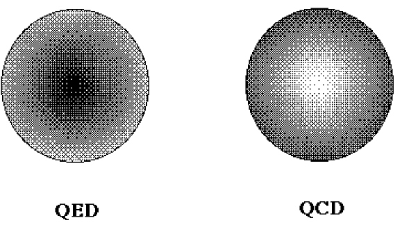
Figure 2.5: The effective charge distribution around an electric charge (QED) and colour charge (QCD). At higher $Q^{2}$ one probes smaller distances, thus observing a larger (smaller) effective charge, i.e. a larger (smaller) coupling constant in QED (QCD).

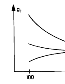
Figure 2.6: Running of the three coupling constants in the Standard Model owing to the different space charge distributions (compare fig. 2.5.

2.5 Running Coupling Constants

In a Quantum Field Theory the coupling constants are only effective constants at a certain energy. They are energy, or equivalently distance dependent through virtual corrections, both in QED and in QCD.

Figure 2.7: Loop corrections in QED (a) and QCD (b). In QED only the fermions contribute in the loops, which causes a screening of the bare charge. In QCD also the bosons contribute through the gluon selfinteraction, which enhances the bare charge. This antiscreening dominates over the screening.

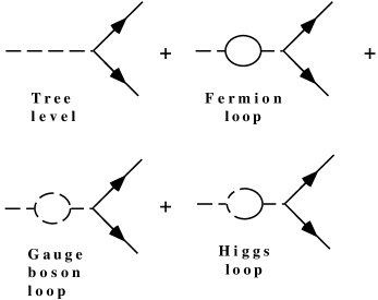
Figure 2.8: First order vacuum polarization diagrams.

However, in QED the coupling constant increases as function of $Q^{2}$, while in QCD the coupling constant decreases. A simple picture for this behaviour is the following:

• The electric field around a pointlike electric charge diverges like $1/r$. In such a strong field electron-positron pairs can be created with a lifetime determined by Heisenberg’s uncertainty relations. These virtual ${e^{+}e^{-}}$ pairs orient themselves in the electric field, thus giving rise to vacuum polarization, just like the atoms in a dielectric are polarized by an external electric field. This vacuum polarization screens the “bare” charge, so at a large distance one observes only an effective charge. This causes deviations from Coulomb’s law, as observed in the well-known Lamb shift of the energy levels of the hydrogen atom. If the electric charge is probed at higher energies (or shorter distances), one penetrates the shielding from the vacuum polarization deeper and observes more of the bare charge, or equivalently one observes a larger coupling constant.

• In QCD the situation is more complicated: the colour charge is surrounded by a cloud of gluons and virtual $q\overline{q}$  pairs; since the gluons themselves carry a colour charge, one has two contributions: a shielding of the bare charge by the $q\overline{q}$  pairs and an increase of the colour charge by the gluon cloud. The net effect of the vacuum polarization is an increase of the total colour charge, provided not too many $q\overline{q}$ pairs contribute, which is the case if the number of generations is below 16, see hereafter. If one probes this charge at smaller distances, one penetrates part of the “antishielding”, thus observing a smaller colour charge at higher energies. So it is the fact that gluons carry colour themselves which makes the coupling decrease at small distances (or high energies). This property is called asymptotic freedom and it explains why in deep inelastic lepton-nucleus scattering experiments the quarks inside a nucleus appear quasi free in spite of the fact that they are tightly bound inside a nucleus. The increase of $\alpha_{s}$  at large distances explains qualitatively why it is so difficult to separate the quarks inside a hadron: the larger the distance the more energy one needs to separate them even further. If the energy of the colour field is too high, it is transformed into mass, thus generating new quarks, which then recombine with the old ones to form new hadrons, so one always ends up with a system of hadrons instead of free quarks.

The space charges from the virtual pairs surrounding an electric charge and colour charge are shown schematically in fig. 2.5. The different vacuum polarizations lead to the energy dependence of the coupling constants sketched in fig. 2.6. The colour field becomes infinitely dense at the QCD scale $\Lambda\approx 200$ MeV (see hereafter). So the confinement radius of typical hadrons is $\cal{O}$(200 MeV) or one Fermi ($10^{-13}$ cm).

The vacuum polarization effects can be calculated from the loop diagrams to the gauge bosons. The main difference between the charge distribution in QED and QCD originates from the diagrams shown in fig. 2.7. In addition one has to consider diagrams of the type shown in fig. 2.8. The ultraviolet divergences ($Q^{2}\rightarrow\infty$) in these diagrams can be absorbed in the coupling constants in a renormalizable theory. All other divergences are canceled at the amplitude level by summing the appropriate amplitudes. The first step in such calculations is the regularization of the divergences, i.e. separating the divergent parts in the mathematical expressions. The second step is the renormalization of physical quantities, like charge and mass, to absorb the divergent parts of the amplitudes, i.e. replace the “bare” quantities of the theory with measured quantities. For example, the loop corrections to the photon propagator diverge, if the momentum transfer $k$ in the loop is integrated to infinity. If one introduces a cutoff $\mu_{0}$ for large values of $k$, one finds for the regularized amplitude of the sum of the Born term $M_{0}$ and the loop corrections[26]:

$$M^{1}=e^{2}\left(1-\frac{\alpha}{3\pi}\ln\frac{\mu_{0}^{2}}{m^{2}}\right)\left(1+\frac{\alpha}{3\pi}\ln\frac{Q^{2}}{m^{2}}\right)\;M^{0}~{}{\rm for}~{}Q^{2}>>m^{2}$$ (2.33)

The divergent part depending on the cutoff parameter $\mu_{0}$ disappears, if one replaces the “bare” charge $e$ by the renormalized charge $e_{R}$:

$$e_{R}^{2}\equiv e^{2}\left(1-\frac{\alpha}{3\pi}\ln\frac{\mu_{0}^{2}}{m^{2}}\right)$$ (2.34)

i.e. the “bare” charge, occurring in the Dirac equation, is renormalized to a measurable quantity $e_{R}$. For $e_{R}$ one usually takes the Thomson limit for Compton scattering, i.e. $\gamma e\rightarrow\gamma e$ for $k\rightarrow 0$:

$$\sigma_{T}=\frac{8\pi}{3}\frac{\alpha^{2}}{m_{e}^{2}}$$ (2.35)

with $\alpha={e_{R}^{2}}/{4\pi}=1/137.036$ and $m_{e}=0.00051$ GeV.

After regularization and renormalization to a measured quantity (in this case using the so called “on shell” scheme, i.e. one uses the mass and charge of a free electron as measured at low energy), one is left with a $Q^{2}$ dependent but finite part of the vacuum polarization. This can be absorbed in a $Q^{2}$ dependent coupling constant, which in case of QED becomes for $Q^{2}>>m^{2}$:

$$\alpha(Q^{2})=\alpha\left(1+\frac{\alpha}{3\pi}\ln\frac{Q^{2}}{m^{2}_{e}}\right)$$ (2.36)

If one sums more loops, this yields terms $(\frac{\alpha}{3\pi})^{n}(\ln\frac{Q^{2}}{m_{e}^{2}})^{m}$ and retaining only the leading logarithms (i.e. n=m), these terms can be summed to:

$$\alpha(Q^{2})=\frac{\alpha}{(1-\frac{\alpha}{3\pi}\ln\frac{Q^{2}}{m_{e}^{2}})}$$ (2.37)

since

$$\sum_{n=0}^{\infty}x^{n}=\frac{1}{1-x}.$$ (2.38)

Of course, the total $Q^{2}$ dependence is obtained by summing over all possible fermion loops in the photon propagator.

These vacuum polarization effects are non-negligible. For example, at LEP accelerator energies $\alpha$ has increased from its low energy value $1/137$ to 1/128 or about 6%.

The diagrams of fig. 2.7b yield similarly to eq. 2.37:

$${\alpha_{s}}(Q^{2})={\alpha_{s}}(\mu^{2})\left[1+\frac{{\alpha_{s}}(\mu^{2})}{4\pi}\left(11-\frac{2N_{f}}{3}\right)\ln\frac{Q^{2}}{\mu^{2}}\right]^{-1}$$ (2.39)

Note that $\alpha_{s}$  decreases with increasing $Q^{2}$ if $11-2N_{f}/3>0$ or $N_{f}<16$, thus leading to asymptotic freedom at high energy. This is in contrast to the $Q^{2}$ dependence of $\alpha(Q^{2})$ in eq. 2.37, which increases with increasing $Q^{2}$. Since $\alpha_{s}$  becomes infinite at small $Q^{2}$, one cannot take this scale as a reference scale. Instead one could choose as renormalization point the “confinement scale” $\Lambda$, i.e. ${\alpha_{s}}\rightarrow\infty$, if $Q^{2}\rightarrow\Lambda$. In this case eq. 2.39 becomes independent of $\mu$, since the 1 in brackets becomes negligible, so one obtains:

$${\alpha_{s}}(Q^{2})=\frac{4\pi}{(11-\frac{2n_{f}}{3})\ ln\frac{Q^{2}}{\Lambda^{2}}}$$ (2.40)

The definition of $\Lambda$ depends on the renormalization scheme. The most widely used scheme is the $\overline{MS}$ scheme[27], which we will use here. Other schemes can be used as well and simple relations between the definitions of $\Lambda$ exist[28].

The higher order corrections are usually calculated with the renormalization group technique, which yields for the $\mu$ dependence of a coupling constant $\alpha$ :

$$\mu\frac{\partial\alpha}{\partial\mu}=\beta_{0}\alpha^{2}+\beta_{1}\alpha^{3}+\beta_{2}\alpha^{4}+...$$ (2.41)

The first two terms in this perturbative expansion are renormalization-scheme independent. Their specific values are given in the appendix. The first order solution of eq. 2.41 is simple:

$$\frac{1}{\alpha(Q^{2})}=\frac{1}{\alpha(Q^{2}_{0})}-\beta_{0}\ln(\frac{Q^{2}}{Q_{0}^{2}})$$ (2.42)

where $Q^{2}_{0}$ is a reference energy. One observes a linear relation between the change in the inverse of the coupling constant and the logarithm of the energy. The slope depends on the sign of $\beta_{0}$, which is positive for QED, but negative for QCD, thus leading to asymptotic freedom in the latter case. The second order corrections are so small, that they do not change this conclusion. Higher order terms depend on the renormalization prescription. In higher orders there are also corrections from Higgs particles and gauge bosons in the loops. Therefore the running of a given coupling constant depends slightly on the value of the other coupling constants and the Yukawa couplings. These higher order corrections cause the RGE equations to be coupled, so one has to solve a large number of coupled differential equations. All these equations are summarized in the appendix.

Chapter 3 Grand Unified Theories.

3.1 Motivation

The Standard Model describes all observed interactions between elementary particles with astonishing precision. Nevertheless, it cannot be considered to be the ultimate theory because the many unanswered questions remain a problem. Among them:

• The Gauge Problem
  Why are there three independent symmetry groups?

• The Parameter Problem
  How can one reduce the number of free parameters? (At least 18 from the couplings, the mixing parameters, the Yukawa couplings and the Higgs potential.)

• The Fermion Problem
  Why are there three generations of quarks and leptons? What is the origin of the the symmetry between quarks and leptons? Are they composite particles of more fundamental objects?

• The Charge Quantization Problem
  Why do protons and electrons have exactly opposite electric charges?

• The Hierarchy Problem
  Why is the weak scale so small compared with the GUT scale, i.e. why is $M_{W}\approx 10^{-17}~{}M_{Planck}?$

• The Fine-tuning Problem
  Radiative corrections to the Higgs masses and gauge boson masses have quadratic divergences. For example, $\Delta M_{H}^{2}\approx{\cal{O}}(M_{Planck}^{2})$. In other words, the corrections to the Higgs masses are many orders of magnitude larger than the masses themselves, since they are expected to be of the order of the electroweak gauge boson masses. This requires extremely unnatural fine-tuning in the parameters of the Higgs potential. This “fine-tuning” problem is solved in the supersymmetric extension of the SM, as will be discussed afterwards.

3.2 Grand Unification

The problems mentioned above can be partly solved by assuming the symmetry groups $SU(3)_{C}\otimes SU(2)_{L}\otimes U(1)_{Y}$  are part of a larger group $G$, i.e.

$$G\supset{SU(3)_{C}\otimes\-SU(2)_{L}\otimes\-U(1)_{Y}}.$$ (3.1)

The smallest group $G$ is the SU(5) group[29], so the minimal extension of the SM towards a GUT is based on the $SU(5)$ group. Throughout this paper we will only consider this minimal extension. The group $G$ has a single coupling constant for all interactions and the observed differences in the couplings at low energy are caused by radiative corrections. As discussed before, the strong coupling constant decreases with increasing energy, while the electromagnetic one increases with energy, so that at some high energy they will become equal. Since the changes with energy are only logarithmic (eq. 2.42), the unification scale is high, namely of the order of $10^{15}-10^{16}$ GeV, depending on the assumed particle content in the loop diagrams.

In the $SU(5)$ group[29] the 15 particles and antiparticles of the first generation can be fit into the $\overline{5}$-plet and 10-plet:

$$\overline{5}=\left(\begin{array}[]{c}d_{g}^{C}\\ d_{r}^{C}\\ d_{b}^{C}\\ e^{-}\\ -\nu_{e}\end{array}\right)~{}~{}10=\frac{1}{\sqrt{2}}\left(\begin{array}[]{ccccc}0&+u_{b}^{C}&-u_{r}^{C}&-u_{g}&-d_{g}\\ -u_{b}^{C}&0&+u_{g}^{C}&-u_{r}&-d_{r}\\ +u_{r}^{C}&-u_{g}^{C}&0&-u_{b}&-d_{b}\\ +u_{g}&+u_{r}&+u_{b}&0&-e^{+}\\ +d_{g}&+d_{r}&+d_{b}&+e^{+}&0\end{array}\right)_{L}$$ (3.2)

The superscript $C$ indicates the charge conjugated particle, i.e. the antiparticle and all particles are chosen to be left-handed, since a left-handed antiparticle transforms like a right-handed particle. Thus the superscript $C$ implies a right-handed singlet with weak isospin equal zero.

With this multiplet structure the sum of the quantum numbers $Q$, $T_{3}$ and $Y$ is zero within one multiplet, as required, since the corresponding operators are represented by traceless matrices.

Note that there is no space for the antineutrino in these multiplets, so within the minimal $SU(5)$ the neutrino must be massless, since for a massive particle the right-handed helicity state is also present. Of course, it is possible to put a right-handed neutrino into a singlet representation.

$SU(5)$ rotations can be represented by $5\times 5$ matrices. Local gauge invariance requires the introduction of $N^{2}-1=24$ gauge fields (the “mediators”), which cause the interactions between the matter fields. The gauge fields transform under the adjoint representation of the $SU(5)$ group, which can be written in matrix form as (compare eqns. 2.7 and 2.3):

$$24=\left(\begin{array}[]{ccc|cc}G_{11}-\frac{2B}{\sqrt{30}}&G_{12}&G_{13}&X_{1}^{C}&Y_{1}^{C}\\ G_{21}&G_{22}-\frac{2B}{\sqrt{30}}&G_{23}&X_{2}^{C}&Y_{2}^{C}\\ G_{31}&G_{32}&G_{33}-\frac{2B}{\sqrt{30}}&X_{3}^{C}&Y_{3}^{C}\\ \hline\cr X_{1}&X_{2}&X_{3}&\frac{W^{3}}{\sqrt{2}}+\frac{3B}{\sqrt{30}}&W^{+}\\ Y_{1}&Y_{2}&Y_{3}&W^{-}&-\frac{W^{3}}{\sqrt{2}}+\frac{3B}{\sqrt{30}}\\ \end{array}\right)$$ (3.3)

The $G$’s represent the gluon fields of equation 2.3, while the $W$’s and $B$’s are the gauge fields of the $SU(2)$ symmetry groups. The $X$ and $Y$’s are new gauge bosons, which represent interactions, in which quarks are transformed into leptons and vice-versa, as should be apparent if one operates with this matrix on the $\overline{5}$-plet. Consequently, the $X$ ($Y$) bosons, which couple to the electron (neutrino) and $d$-quark must have electric charge $4/3$ (1/3).

Figure 3.1: GUT proton decays through the exchange of $X$ and $Y$ gauge bosons.

3.3 $SU(5)$ predictions

3.3.1 Proton decay

The $X$ and $Y$ gauge bosons can introduce transitions between quarks and leptons, thus violating lepton and baryon number. This can lead to the following proton and neutron decays (see fig. 3.1):

$$\begin{array}[]{cc}p\rightarrow e^{+}\pi^{0}&n\rightarrow e^{+}\pi^{-}\\ p\rightarrow e^{+}\rho^{0}&n\rightarrow e^{+}\rho^{-}\\ p\rightarrow e^{+}\omega^{0}&n\rightarrow{\nu}\omega^{0}\\ p\rightarrow e^{+}\eta&n\rightarrow\overline{\nu}\pi^{0}\\ p\rightarrow\overline{\nu}\pi^{+}&n\rightarrow\overline{\nu}_{\mu}K^{0}\\ p\rightarrow\overline{\nu}\rho^{+}&\\ p\rightarrow\overline{\nu}_{\mu}K^{+}\end{array}$$ (3.4)

The decays with kaons in the final state are allowed through flavour mixing, i.e. the interaction eigenstates are not necessarily the mass eigenstates.

For the lifetime of the nucleon one writes in analogy to muon decay:

$$\tau_{p}\approx\frac{M^{4}_{X}}{\alpha_{5}^{2}m_{p}^{5}}$$ (3.5)

The proton mass $m_{p}$ to the fifth power originates from the phase space in case the final states are much lighter than the proton, which is the case for the dominant decay mode: $p\rightarrow e^{+}\pi_{0}$. After this prediction of an unstable proton in grand unified theories, a great deal of activity developed and the lower limit on the proton life time increased to[30]

$$\tau_{p}>5\cdot 10^{32}~{}{\rm yrs}$$ (3.6)

for the dominant decay mode $p\rightarrow e^{+}\pi^{0}$. From equation 3.5 this implies (for $\alpha_{5}=1/24$, see chapter 6)

$$M_{X}\geq 10^{15}~{}{\rm GeV.}$$ (3.7)

From the extrapolation of the couplings in the $SU(5)$ model to high energies one expects the unification scale to be reached well below $10^{15}$ GeV, so the proton lifetime measurements exclude the minimal $SU(5)$ model as a viable GUT. As will be discussed later, the supersymmetric extension of the $SU(5)$ model has the unification point well above $10^{15}$ GeV.

3.3.2 Baryon Asymmetry

The heavy gauge bosons responsible for the unified force cannot be produced with conventional accelerators, but energies above $10^{15}$ were easily accessible during the birth of our universe. This could have led to an excess of matter over antimatter right at the beginning, since the $X$ and $Y$ bosons can decay into pure matter, e.g. $X\rightarrow uu$, which is allowed because the charge of the $X$ boson is 4/3. As pointed out by Sakharov[31] such an excess is possible if both C and CP are violated, if the baryon number B is violated, and if the process goes through a phase of non-equilibrium. All three conditions are possible within the $SU(5)$ model. The non-equilibrium phase happens if the hot universe cools down and arrives at a temperature, too low to generate $X$ and $Y$ bosons anymore, so only the decays are possible. Since the CP violation is expected to be small, the excess of matter over antimatter will be small, so most of the matter annihilated with antimatter into enormous number of photons. This would explain why the number of photons over baryons is so large:

$$\frac{N_{\gamma}}{N_{b}}\approx 10^{10}$$ (3.8)

However, later it was realized that the electroweak phase transition may wash out any (B+L) excess generated by GUT’s. One then has to explain the observed baryon asymmetry by the electroweak baryogenesis, which is actively studied[32].

3.3.3 Charge Quantization

From the fact that quarks and leptons are assigned to the same multiplet the charges must be related, since the trace of any generator has to be zero. For example, the charge operator Q on the fundamental representation yields:

$$TrQ=Tr(q_{\overline{d}},q_{\overline{d}},q_{\overline{d}},e,0)=0$$ (3.9)

or in other words, in $SU(5)$ the electric charge of the $d$-quark has to be 1/3 of the charge of an electron! Similarly, one finds the charge of the $u$-quark is 2/3 of the positron charge, so the total charge of the proton (=$uud$) has to be exactly opposite to the charge of an electron.

Figure 3.2: Radiative corrections to particle masses.

3.3.4 Prediction of $\;\sin^{2}\theta_{W}$

If the $SU(2)$ and $U(1)$ groups have equal coupling constants, the electroweak mixing angle can be calculated easily, since it is given by the ratio $g^{\prime\;2}/(g^{2}+g^{\prime\;2})$ (see eq. 2.25), which would be 1/2 for equal coupling constants. However, the argument is slightly more subtle, since for unitary transformations the rotation matrices have to be normalized such that

$$Tr\;{F_{k}F_{l}}=\delta_{kl}.$$ (3.10)

This normalization is not critical in case one has independent coupling constants for the subgroups, since a “wrong” normalization for a rotation matrix can always be corrected by a redefinition of the corresponding coupling constants, as is apparent from equation 2.6. This freedom is lost, if one has a single coupling constant, so one has to be careful about the relative normalization. It turns out, that the Gell-Mann and Pauli rotation matrices of the $SU(3)$ and $SU(2)$ groups have the correct normalization, but the normalization of the weak hypercharge operator needs to be changed. Defining $1/2Y_{W}=CT_{0}$ and substituting this into the Gell-Mann-Nishijima relation 2.2 yields:

$$Q=T_{3}+CT_{0}$$ (3.11)

Requiring the same normalization for $T_{3}$ and $T_{0}$ implies from equation 3.10:

$$Tr\;{Q^{2}}=(1+C^{2})~{}Tr\;{T_{3}^{2}}$$ (3.12)

or inserting numbers from the $\overline{5}$-plet of $SU(5)$ yields:

$$1+C^{2}=\frac{Tr\;Q^{2}}{Tr\;T_{3}^{2}}=\frac{3\cdot 1/9+1}{2\cdot 1/4}=\frac{8}{3}.$$ (3.13)

Replacing in the covariant derivative (eq. 2.6) $1/2Y_{W}$ with $CT_{0}$ implies $g^{\prime}CT_{0}\equiv g_{5}T_{0}$ or:

$$g_{5}=Cg^{\prime},$$ (3.14)

where $C^{2}={5}/{3}$ from eq. 3.13. With this normalization the electroweak mixing angle after unification becomes:

$${\;\sin^{2}\theta_{W}}=\frac{g^{\prime 2}}{(g^{2}+g^{\prime\;2})}=\frac{g_{5}^{2}/C^{2}}{(g_{5}^{2}+g^{2}_{5}/C^{2})}=\frac{1}{1+C^{2}}=\frac{3}{8}.$$ (3.15)

The manifest disagreement with the experimental value of 0.23 at low energies brought the $SU(5)$ model originally into discredit, until it was noticed that the running of the couplings between the unification scale and low energies could reduce the value of ${\;\sin^{2}\theta_{W}}$ considerably. As we will show in the last chapter, with the very precise measurement of ${\;\sin^{2}\theta_{W}}$ at LEP, unification of the three coupling constants within the $SU(5)$ model is excluded, and just as in the case of the proton life time, supersymmetry comes to the rescue and unification is perfectly possible within the supersymmetric extension of $SU(5)$.

Note that the prediction of ${\;\sin^{2}\theta_{W}}=3/8$ is not specific to the $SU(5)$ model, but is true for any group with ${SU(3)_{C}\otimes\-SU(2)_{L}\otimes\-U(1)_{Y}}$ as subgroups, implying that $Q$, $T_{3}$ and $Y_{W}$ are generators with traces equal zero and thus leading to the predictions given above.

3.4 Spontaneous Symmetry Breaking in $SU(5)$

The $SU(5)$ symmetry is certainly broken, since the new force corresponding to the exchange of the $X$ and $Y$ bosons would lead to very rapid proton decay, if these new gauge bosons were massless. As mentioned above, from the limit on the proton life time these $SU(5)$ gauge boson have to be very heavy, i.e. masses above $10^{15}$ GeV. The generation of masses can be obtained again in a gauge invariant way via the Higgs mechanism. The Higgs field is chosen in the adjoint representation $\underline{24}$ and the minimum $<\Phi_{24}>$ can be chosen in the following way:

$$<\Phi_{24}>=v_{24}~{}\left(\begin{array}[]{ccc|cc}1&&&&\\ &1&&&\\ &&1&&\\ \hline\cr&&&-\frac{3}{2}&\\ &&&&-\frac{3}{2}\end{array}\right)$$ (3.16)

The 12 X,Y gauge bosons of the $SU(5)$ group require a mass:

$$M_{X}^{2}=M_{Y}^{2}=\frac{25}{8}g_{5}^{2}v_{24}^{2}$$ (3.17)

after ‘eating’ 12 of the 24 scalar fields in the adjoint representation, thus providing the longitudinal degrees of freedom. The field $\Phi_{24}$ is invariant under the rotations of the ${SU(3)_{C}\otimes\-SU(2)_{L}\otimes\-U(1)_{Y}}$ group, so this symmetry is not broken and the corresponding gauge bosons, including the $W$ and $Z$ bosons, remain massless. after the first stage of $SU(5)$ symmetry breaking.

The usual breakdown of the electroweak symmetry to $SU(3)_{C}\otimes U(1)_{em}$ is achieved by a 5-plet $\Phi_{5}$ of Higgs fields, for which the minimum of the effective potential can be chosen at:

$$<\Phi_{5}>={v_{5}}\left(\begin{array}[]{c}0\\ 0\\ 0\\ 0\\ 1\end{array}\right)$$ (3.18)

The fourth and fifth component of $\Phi_{5}$ correspond to the $SU(2)$ doublet $(\Phi^{+},\Phi^{0})$ of the SM (see eq. 2.10). Since the total charge in a representation has to be zero again, the first triplet of complex fields in $\Phi_{5}$, which transforms as (3,1)_-2/3 and $(3^{*},1)_{2/3}$, must have charge $|1/3|$. Since they couple to all fermions with mass, they can induce proton decay:

$$u+d\rightarrow H^{1/3}\rightarrow\begin{array}[]{c}e^{+}+\overline{u}\\ \overline{\nu}_{e}+\overline{d}\end{array}$$ (3.19)

Such decays can be suppressed only by sufficiently high masses of the coloured Higgs triplet. These can obtain high masses through interaction terms between $\Phi_{5}$ and $\Phi_{24}$.

Note that from eq. 3.17 $<\Phi_{24}>$ has to be of the order of $M_{X}$, while $\Phi_{5}$ has to be of the order of $M_{W}$, since

$$M_{W}^{2}=\frac{1}{2}(g_{5}v_{5})^{2}$$ (3.20)

and

$$M_{Z}=\frac{M_{W}}{\cos\theta_{W}}$$ (3.21)

or more precisely $v_{5}=1/\sqrt{G_{F}}$= 174 GeV. The minimum of the Higgs potential involves both $\Phi_{5}$ and $\Phi_{24}$. Despite this mixing, the ratio $v_{5}/v_{24}\approx 10^{-13}$ has to be preserved (hierarchy problem). Radiative corrections spoil usually such a fine-tuning, so $SU(5)$ is in trouble. As will be discussed later, also here supersymmetry offers solutions for both this fine-tuning and the hierarchy problem.

3.5 Relations between Quark and Lepton Masses

The Higgs 5-plet $\Phi_{5}$ can be used to generate fermion masses. Since the $\overline{5}$-plet of the matter fields contains both leptons and down-type quarks, their masses are related, while the up-type quark masses are free parameters. At the GUT scale one expects:

$$m_{d} = m_{e}$$ (3.22)

$$m_{s} = m_{\mu}$$ (3.23)

$$m_{b} = m_{\tau}$$ (3.24)

Unfortunately the masses of the light quarks have large uncertainties from the binding energies in the hadrons, but the b-quark mass can be correctly predicted from the $\tau$-mass after including radiative corrections (see fig. 3.2 for typical graphs).

Since the corrections from graphs involving the strong coupling constant $\alpha_{s}$ are dominant, one expects in first order[33]

$$\frac{m_{b}}{m_{\tau}}={\cal{O}}\left(\frac{\alpha_{s}(m_{b})}{\alpha_{s}(M_{X})}\right)={\cal{O}}(3)$$ (3.25)

More precise formulae are given in the appendix and will be used in the last chapter in a quantitative analysis, since the b-quark mass gives a rather strong constraint on the evolution of the couplings and through the radiative corrections involving the Yukawa couplings on the top quark mass.

Chapter 4 Supersymmetry

4.1 Motivation

Supersymmetry[13, 14] presupposes a symmetry between fermions and bosons, which can be realized in nature only if one assumes each particle with spin j has a supersymmetric partner with spin j-1/2. This leads to a doubling of the particle spectrum (see table 4.1), which are assigned to two supermultiplets: the vector multiplet for the gauge bosons and the chiral multiplet for the matter fields. Unfortunately the supersymmetric particles or “sparticles” have not been observed so far, so either supersymmetry is an elegant idea, which has nothing to do with reality, or supersymmetry is not an exact symmetry, in which case the sparticles can be heavier than the particles.

$$\begin{array}[]{|c|c||c|c|}\hline\cr\vrule\lx@intercol\hfil\mbox{VECTOR MULTIPLET }\hfil\lx@intercol\vrule\lx@intercol\vrule\lx@intercol&\vrule\lx@intercol\hfil\mbox{CHIRAL MULTIPLET}\hfil\lx@intercol\vrule\lx@intercol\\ \hline\cr\hline\cr\rule{0.0pt}{17.07182pt}J=1&J=1/2&J=1/2&J=0\\ \hline\cr\rule{0.0pt}{17.07182pt}g&\tilde{g}&Q_{L},U_{L}^{C},D_{L}^{C}&\tilde{Q}_{L},\tilde{U}_{L}^{C},\tilde{D}_{L}^{C}\\ \rule{0.0pt}{17.07182pt}W^{\pm},W^{0}&\tilde{W}^{\pm},\tilde{W}^{0}&L_{L},E_{L}^{C}&\tilde{L}_{L},\tilde{E}_{L}^{C}\\ \rule{0.0pt}{17.07182pt}B&\tilde{B}&\tilde{H}_{1},\tilde{H}_{2}&H_{1},H_{2}\\ \hline\cr\end{array}$$

Table 4.1: Assignment of gauge fields to the vector superfield and the matter fields to the chiral superfield.

Many people opt for the latter way out, since there are many good reasons to believe in supersymmetry:

• SUSY solves the fine-tuning problem
  As mentioned before, the radiative corrections in the $SU(5)$ model have quadratic divergences from the diagrams in fig. 2.8, which lead to $\Delta M_{H}^{2}\approx{\cal{O}}(M_{X}^{2})$, where $M_{X}$ is a cutoff scale, typically the unification scale if no other scales introduce new physics beforehand.

  However, in SUSY the loop corrections contain both fermions (F) and bosons (B) in the loops, which according to the Feynman rules contribute with an opposite sign, i.e.

  $$\Delta M_{H}^{2}\approx{\cal{O}}(\alpha)~{}|M_{B}^{2}-M_{F}^{2}|\approx{\cal{O}}(10^{-2})M_{SUSY}^{2}$$ (4.1)

  where $M_{SUSY}$ is a typical SUSY mass scale. In other words, the fine-tuning problem disappears, if the SUSY partners are not too heavy compared with the known fermions. An estimate of the required SUSY breaking scale can be obtained by considering that the masses of the weak gauge bosons and Higgs masses are both obtained by multiplying the vacuum expectation value of the Higgs field (see previous chapter) with a coupling constant, so one expects $M_{W}\approx M_{H}$. Requiring that the radiative corrections are not much larger than the masses themselves, i.e. $\Delta M_{W}<M_{W}$, or replacing $M_{W}$ by $M_{H}$, $\Delta M_{H}<{\cal{O}}(10^{2})$, yields after substitution into eq. 4.1:

  $$M_{SUSY}\leq 10^{3}~{}{\rm GeV.}$$ (4.2)

• SUSY offers a solution for the hierarchy problem
  The possible explanation for the small ratio $M_{W}^{2}/M_{X}^{2}\approx 10^{-28}$ is simple in SUSY models: large radiative corrections from the top-quark Yukawa coupling to the Higgs sector drive one of the Higgs masses squared negative, thus changing the shape of the effective potential from the parabolic shape to the Mexican hat (see fig. 2.4) and triggering electroweak symmetry breaking[34]. Since radiative corrections are logarithmic in energy, this automatically leads to a large hierarchy between the scales. In the SM one could invoke a similar mechanism for the triggering of electroweak symmetry breaking, but in that case the quadratic divergences in the radiative corrections would upset the argument.

  In the MSSM the electroweak scale is governed by the starting values of the parameters at the GUT scale and the top-quark mass. This strongly constrains the SUSY mass spectrum, as will be discussed in the last chapter.

  

  Figure 4.1: Evolution of the inverse of the three coupling constants in the Standard Model (SM) (top) and in the supersymmetric extension of the SM (MSSM) (bottom). Only in the latter case unification is obtained. The SUSY particles are assumed to contribute only above the effective SUSY scale ${M_{SUSY}}$ of about one TeV, which causes the change in slope in the evolution of the couplings. The 68% C.L. for this scale is indicated by the vertical lines (dashed). The evolution of the couplings was calculated in second order (see section A.2 of the appendix with the constants $\beta_{i}$ and $\beta_{ij}$ calculated for the MSSM above ${M_{SUSY}}$ in the bottom part and for the SM elsewhere). The thickness of the lines represents the error in the coupling constants.

  

  Figure 4.2: $\chi^{2}$ distribution for ${M_{SUSY}}$ and${M_{GUT}}$.

• SUSY yields unification of the coupling constants
  After the precise measurements of the ${SU(3)_{C}\otimes\-SU(2)_{L}\otimes\-U(1)_{Y}}$ coupling constants, the possibility of coupling constant unification within the SM could be excluded, since after extrapolation to high energies the three coupling constants would not meet in a single point. This is demonstrated in the upper part of fig. 4.1, which shows the evolution of the inverse of the couplings as function of the logarithm of the energy. In this presentation the evolution becomes a straight line in first order, as is apparent from the solution of the RGE (eqn. 2.42). The second order corrections, which have been included in fig. 4.1 by using eqs. A.20 from the appendix, are so small, that they cause no visible deviation from a straight line.

  A single unification point is excluded by more than 8 standard deviations. The curve $1/\alpha_{3}$ meets the crossing point of the other two coupling constants only for a starting value at $\alpha_{s}(M_{Z})$ = 0.07, while the measured value is $0.12\pm 0.006$[22]. This is an exciting result, since it means unification can only be obtained, if new physics enters between the electroweak and the Planck scale!

  It turns out that within the SUSY model perfect unification can be obtained if the SUSY masses are of the order of one TeV. This is shown in the bottom part of fig. 4.1; the SUSY particles are assumed to contribute effectively to the running of the coupling constants only for energies above the typical SUSY mass scale, which causes the change in the slope of the lines near one TeV. From a fit requiring unification one finds for the breakpoint ${M_{SUSY}}$ and the unification point ${M_{GUT}}$[35, 36]:

  $${M_{SUSY}} = 10^{3.4~{}\pm~{}0.9~{}~{}\pm~{}0.4}~{}{{\rm GeV}}$$ (4.3)

  $${M_{GUT}} = 10^{15.8~{}\pm~{}0.3~{}\pm~{}0.1}~{}{{\rm GeV}}$$ (4.4)

  $${\alpha_{GUT}}^{-1} = 26.3~{}\pm~{}1.9~{}\pm~{}1.0,$$ (4.5)

  where ${\alpha_{GUT}}\equiv g_{5}^{2}/4\pi$. The first error originates from the uncertainty in the coupling constant, while the second error is due to the uncertainty in the mass splittings between the SUSY particles. The $\chi^{2}$ distributions of ${M_{SUSY}}$ and ${M_{GUT}}$ for the fit in the bottom part of fig. 4.1 are shown in fig. 4.2. These figures are an update of the published figures using the newest values of the coupling constants, as shown in the figure[36].

  Note that the parametrisation of the SUSY mass spectrum with a single mass scale is not adequate and leads to uncertainties. However, the errors in the coupling constants (mainly in ${\alpha_{s}}$) are large and the uncertainties from mass splittings between the sparticles are more than a factor two smaller (see eq. 4.3). In the last chapter the unification including a more detailed treatment of the mass splittings will be studied.

  One can ask: ’What is the significance of this observation? For many people it was the first “evidence” for supersymmetry, especially since ${M_{SUSY}}$ was found in the range where the fine-tuning problem does not reappear (see eq. 4.2). Consequently the results triggered a revival of the interest in SUSY, as was apparent from the fact that ref. [11] with the $\chi^{2}$ fit of the unification of the coupling constants, as exemplified in figs. 4.1 and 4.2, reached the Top-Ten of the citation list, thus leading to discussions in practically all popular journals[37].

  Non-SUSY enthusiasts were considering unification obvious: with a total of three free parameters (${M_{GUT}},~{}{\alpha_{GUT}}$ and ${M_{SUSY}}$) and three equations one can naively always find a solution. The latter statement is certainly not true: searching for other types of new physics with the masses as free particles yields only rarely unification, especially if one requires in addition that the unification scale is above $10^{15}$ GeV in order to be consistent with the proton lifetime limits and below the Planck scale in order to be in the regime where gravity can be neglected. From the 1600 models tried, only a handful yielded unification[35]. The reason is simple: introducing new particles usually alters all three couplings simultaneously, thus giving rise to strong correlations between the slopes of the three lines. For example, adding a fourth family of particles with an arbitrary mass will never yield unification, since it changes the slopes of all three coupling by the same amount, so if with three families unification cannot be obtained, it will not work with four families either, even if one has an additional free parameter! Nevertheless, unification does not prove supersymmetry, it only gives an interesting hint. The real proof would be the observation of the sparticles.

• Unification with gravity
  The space-time symmetry group is the Poincaré group. Requiring local gauge invariance under the transformations of this group leads to the Einstein theory of gravitation. Localizing both the internal and the space-time symmetry groups yields the Yang-Mills gauge fields and the gravitational fields. This paves the way for the unification of gravity with the strong and electroweak interactions. The only non-trivial unification of an internal symmetry and the space-time symmetry group is the supersymmetry group, so supersymmetric theories automatically include gravity[38]. Unfortunately supergravity models are inherently non-renormalizible, which prevents up to now clear predictions. Nevertheless, the spontaneous symmetry breaking of supergravity is important for the low energy spectrum of supersymmetry[39]. The most common scenario is the hidden sector scenario[40], in which one postulates two sectors of fields: the visible sector containing all the particles of the GUT’s described before and the hidden sector, which contains fields which lead to symmetry breaking of supersymmetry at some large scale $\Lambda_{SUSY}$. One assumes that none of the fields in the hidden sector contains quantum numbers of the visible sector, so the two sectors only communicate via gravitational interactions. Consequently, the effective scale of supersymmetry breaking in the visible sector is suppressed by a power of the Planck scale, i.e.

  $${M_{SUSY}}\approx\frac{\Lambda^{n}_{SUSY}}{M^{n-1}_{Planck}},$$ (4.6)

  where $n$ is model-dependent (e.g. $n=2$ in the Polonyi model). Thus the SUSY breaking scale can be large, above $10^{10}$ GeV, while still producing a small breaking scale in the visible sector. In this case the fine-tuning problem can be avoided in a natural way and it is gratifying to see that the first experimental hints for ${M_{SUSY}}$ are indeed in the mass range consistent with eq. 4.2.

  The hidden sector scenario leads to an effective low-energy theory with explicit soft breaking terms, where soft implies that no new quadratic divergences are generated[41]. The soft-breaking terms in string-inspired supergravity models have been studied recently in refs. [42]. A final theory, which simultaneously solves the cosmological constant problem[43] and explains the origin of supersymmetry breaking, needs certainly a better understanding of superstring theory.

• The unification scale in SUSY is large
  As discussed in chapter 3, the limits on the proton lifetime require the unification scale to be above $10^{15}$ GeV, which is the case for the MSSM. In addition, one has to consider proton decay via graphs of the type shown in fig. 4.3. These yield a strong constraint on the mixing in the Higgs sector[44], as will be discussed in detail in the last chapter.

• Prediction of dark matter
  The lightest supersymmetric particle (LSP) cannot decay into normal matter, because of R-parity conservation (see the next section for a definition of R-parity). In addition R-parity forbids a coupling between the LSP and normal matter.

  Consequently, the LSP is an ideal candidate for dark matter[45], which is believed to account for a large fraction of all mass in the universe (see next chapter). The mass of the dark matter particles is expected to be below one TeV[46].

Figure 4.3: Examples of proton decay in the minimal supersymmetric model via wino and Higgsino exchange.

4.2 SUSY interactions

The quantum numbers and the gauge couplings of the particles and sparticles have to be the same, since they belong to the same multiplet structure.

The interaction of the sparticles with normal matter is governed by a new multiplicative quantum number called R-parity, which is needed in order to prevent baryon- and lepton number violation. Remember that quarks, leptons and Higgses are all contained in the same chiral supermultiplet, which allows couplings between quarks and leptons. Such transitions, which could lead to rapid proton decay, are not observed in nature. Therefore, the SM particles are assigned a positive R-parity and the supersymmetric partners are R-odd. Requiring R-parity conservation implies that:

• sparticles can be produced only in pairs

• the lightest supersymmetric particle is stable, since its decay into normal matter would change R-parity.

• the interactions of particles and sparticles can be different. For example, the photon couples to electron-positron pairs, but the photino does not couple to selectron-spositron pairs, since in the latter case the R-parity would change from -1 to +1.

4.3 The SUSY Mass Spectrum

Obviously SUSY cannot be an exact symmetry of nature; or else the supersymmetric partners would have the same mass as the normal particles. As mentioned above, the supersymmetric partners should be not too heavy, since otherwise the hierarchy problem reappears.

Furthermore, if one requires that the breaking terms do not introduce quadratic divergences, only the so-called soft breaking terms are allowed[41].

Using the supergravity inspired breaking terms, which assume a common mass $m_{1/2}$ for the gauginos and another common mass $m_{0}$ for the scalars, leads to the following breaking term in the Lagrangian (in the notation of ref. [47]):

$${\cal L}_{Breaking} = -m_{0}^{2}\sum_{i}|\varphi_{i}|^{2}-m_{1/2}\sum_{\alpha}\lambda_{\alpha}\lambda_{\alpha}$$ (4.7)

$$- Am_{0}\left[h^{u}_{ab}Q_{a}U^{c}_{b}H_{2}+h^{d}_{ab}Q_{a}D^{c}_{b}H_{1}+h^{e}_{ab}L_{a}E^{c}_{b}H_{1}\right]-Bm_{0}\left[\mu H_{1}H_{2}\right].$$ (4.8)

Here

$h^{u,d,e}_{ab}$	are the Yukawa couplings,  $a,b=1,2,3$ run over the generations
$Q_{a}$	are the SU(2) doublet quark fields
$U_{a}^{c}$	are the SU(2) singlet charge-conjugated up-quark fields
$D_{b}^{c}$	are the SU(2) singlet charge-conjugated down-quark fields
$L_{a}$	are the SU(2) doublet lepton fields
$E_{a}^{c}$	are the SU(2) singlet charge-conjugated lepton fields
$H_{1,2}$	are the SU(2) doublet Higgs fields
$\varphi_{i}$	are all scalar fields
$\lambda_{\alpha}$	are the gaugino fields

The last two terms in ${\cal{L}}_{Breaking}$ originate from the cubic and quadratic terms in the superpotential with A, B and $\mu$ as free parameters. In total we now have three couplings $\alpha_{i}$ and five mass parameters

$$m_{0},~{}m_{1/2},~{}\mu(t),~{}A(t),~{}B(t)$$

with the following boundary conditions at ${M_{GUT}}$ $(t=0)$:

$${\rm scalars:} \tilde{m}^{2}_{Q}=\tilde{m}^{2}_{U}=\tilde{m}^{2}_{D}=\tilde{m}^{2}_{L}=\tilde{m}^{2}_{E}=m_{0}^{2};$$ (4.9)

$${\rm gauginos:} M_{i}=m_{1/2},\ \ \ i=1,2,3;$$ (4.10)

$${\rm couplings:} \tilde{\alpha}_{i}(0)=\tilde{\alpha}_{GUT},\ \ \ i=1,2,3.$$ (4.11)

Here $M_{1}$, $M_{2}$, and $M_{3}$ are the gauginos masses of the $U(1)$, $SU(2)$ and $SU(3)$ groups. In $N=1$ supergravity one expects at the Planck scale $B=A-1$. With these parameters and the initial conditions at the GUT scale the masses of all SUSY particles can be calculated via the renormalization group equations.

4.4 Squarks and Sleptons

The squark and slepton masses all have the same value at the GUT scale. However, in contrast to the leptons, the squarks get additional radiative corrections from virtual gluons (like the ones in fig. 3.2 for quarks), which makes them heavier than the sleptons at low energies. These radiative corrections can be calculated from the corresponding RGE, which have been assembled in the appendix. The solutions are:

$$\tilde{m}^{2}_{E_{L}}(t=66) = m^{2}_{0}+0.52m^{2}_{1/2}-0.27\cos(2\beta)M_{Z}^{2}$$ (4.12)

$$\tilde{m}^{2}_{\nu_{L}}(t=66) = m^{2}_{0}+0.52m^{2}_{1/2}+0.5\cos(2\beta)M_{Z}^{2}$$ (4.13)

$$\tilde{m}^{2}_{E_{R}}(t=66) = m^{2}_{0}+0.15m^{2}_{1/2}-0.23\cos(2\beta)M_{Z}^{2}$$ (4.14)

$$\tilde{m}^{2}_{U_{L}}(t=66) = m^{2}_{0}+6.6m^{2}_{1/2}+0.35\cos(2\beta)M_{Z}^{2}$$ (4.15)

$$\tilde{m}^{2}_{D_{L}}(t=66) = m^{2}_{0}+6.6m^{2}_{1/2}-0.42\cos(2\beta)M_{Z}^{2}$$ (4.16)

$$\tilde{m}^{2}_{U_{R}}(t=66) = m^{2}_{0}+6.2m^{2}_{1/2}+0.15\cos(2\beta)M_{Z}^{2}$$ (4.17)

$$\tilde{m}^{2}_{D_{R}}(t=66) = m^{2}_{0}+6.1m^{2}_{1/2}-0.07\cos(2\beta)M_{Z}^{2},$$ (4.18)

where $\beta$ is the mixing angle between the two Higgs doublets, which will be defined more precisely in section 4.6. The coefficients depend on the couplings as shown explicitly in the appendix. They were calculated for the parameters from the typical fit shown in table 6.1 ($\alpha_{GUT}=1/24.3$, ${M_{GUT}}=2.0\cdot 10^{16}$ GeV and ${\;\sin^{2}\theta_{W}}=0.2324$). For the third generation the Yukawa coupling is not necessarily negligible. If one includes only the correction from the top Yukawa coupling $Y_{t}$, one finds:

$$\tilde{m}^{2}_{b_{R}}(t=66) = \tilde{m}^{2}_{D_{R}}$$ (4.19)

$$\tilde{m}^{2}_{b_{L}}(t=66) = \tilde{m}^{2}_{D_{L}}-0.48m^{2}_{0}-1.21m^{2}_{1/2}$$ (4.20)

$$\tilde{m}^{2}_{t_{R}}(t=66) = \tilde{m}^{2}_{U_{R}}+m_{t}^{2}-0.96m^{2}_{0}-2.42m^{2}_{1/2}$$ (4.21)

$$\tilde{m}^{2}_{t_{L}}(t=66) = \tilde{m}^{2}_{U_{L}}+m_{t}^{2}-0.48m^{2}_{0}-1.21m^{2}_{1/2}$$ (4.22)

The numerical factors have been calculated for $A_{t}(0)=0$ and the explicit dependence on the couplings can be found in the appendix. Note that only the left-handed b-quark gets corrections from the top-quark Yukawa coupling through a loop with a charged Higgsino and a top-quark. The subscripts $L$ or $R$ do not indicate the helicity, since the squarks and sleptons have no spin. The labels just indicate in analogy to the non-SUSY particles, if they are $SU(2)$ doublets or singlets. The mass eigenstates are mixtures of the $L$ and $R$ weak interaction states. Since the mixing is proportional to the Yukawa coupling, we will only consider the mixing for the top quarks. After mixing the mass eigenstates are: (using the same numerical input as for the light quarks):

$$\tilde{m}^{2}_{t_{1,2}}(t=66) = \frac{1}{2}\left[\tilde{m}^{2}_{t_{L}}+\tilde{m}^{2}_{t_{R}}\pm\sqrt{(\tilde{m}^{2}_{t_{L}}-\tilde{m}^{2}_{t_{R}})^{2}+4m^{2}_{t}(A_{t}m_{0}+\mu/\tan\beta)^{2}}\right]$$

$$\approx \frac{1}{2}\left[0.6m_{0}^{2}+9.2m_{1/2}^{2}+2m_{t}^{2}-0.19\cos(2\beta)M_{Z}^{2}\right]$$

$$\pm\frac{1}{2}\sqrt{\left[1.6m_{1/2}^{2}+0.5m_{0}^{2}-0.5\cos(2\beta)M_{Z}^{2}\right]^{2}+4m_{t}^{2}(A_{t}m_{0}+\mu/\tan\beta)^{2}}$$

. (4.23)

where the values of $A_{t}$ and $\mu$ at the weak scale can be calculated as:

$$A_{t}(M_{Z})=4.6A_{t}(0)+1.7\frac{m_{1/2}}{m_{0}}$$ (4.24)

$$\mu(M_{Z})=0.63\mu(0)$$ (4.25)

Note that for large values of $A_{t}(0)$ or $\mu$ combined with a small $\tan\beta$ the splitting becomes large and one of the stop masses can become very small; since the stop mass lower limit is about 46 GeV[48], this yields a constraint on the possible values of $m_{t},~{}{m_{1/2}},~{}{\tan\beta}$ and $\mu$.

Figure 4.4: Typical running of the squark ($\tilde{q}$), slepton ($\tilde{e}_{L}$), and gaugino ($M_{1},~{}M_{2},~{}M_{3}$) masses (solid lines). The dashed lines indicate the running of the four neutralinos and two charginos.

4.5 Charginos and Neutralinos

The solutions of the RGE group equations for the gaugino masses are simple:

$$M_{i}(t)=\frac{\tilde{\alpha}_{i}(t)}{\tilde{\alpha}_{i}(0)}m_{1/2}.$$ (4.26)

Numerically at the weak scale $(t=2\ln({M_{GUT}}/{M_{Z}})=66)$ one finds (see fig. 4.4):

$$M_{3}(\tilde{g}) \approx 2.7m_{1/2},$$ (4.27)

$$M_{2}(M_{Z}) \approx 0.8m_{1/2},$$ (4.28)

$$M_{1}(M_{Z}) \approx 0.4m_{1/2}.$$ (4.29)

Since the gluinos obtain corrections from the strong coupling constant $\alpha_{3}$, they grow heavier than the gauginos of the ${SU(3)_{C}\otimes\-SU(2)_{L}\otimes\-U(1)_{Y}}$ group.

The calculation of the mass eigenstates is more complicated, since both Higgsinos and gauginos are spin 1/2 particles, so the mass eigenstates are in general mixtures of the weak interaction eigenstates. The mixing of the Higgsinos and gauginos, whose mass eigenstates are called charginos and neutralinos for the charged and neutral fields, respectively, can be parametrised by the following Lagrangian:

$${\cal L}_{Gaugino-Higgsino}=-\frac{1}{2}M_{3}\bar{\lambda}_{a}\lambda_{a}-\frac{1}{2}\bar{\chi}M^{(0)}\chi-(\bar{\psi}M^{(c)}\psi+h.c.)$$

where $\lambda_{a},a=1,2,\ldots,8,$ are the Majorana gluino fields and

$$\chi=\left(\begin{array}[]{c}\tilde{B}\\ \tilde{W}^{3}\\ \tilde{H}^{0}_{1}\\ \tilde{H}^{0}_{2}\end{array}\right),\ \ \ \psi=\left(\begin{array}[]{c}\tilde{W}^{+}\\ \tilde{H}^{+}\end{array}\right),$$

are the Majorana neutralino and Dirac chargino fields, respectively. Here all the terms in the Lagrangian were assembled into matrix notation (similarly to the mass matrix for the mixing between $B$ and $W^{0}$ in the SM, eq. 2.4.2). The mass matrices can be written as[14]:

$$M^{(0)}=\left(\begin{array}[]{cccc}M_{1}&0&-M_{Z}\cos\beta{\;\sin\theta_{W}}&M_{Z}\sin\beta{\;\sin\theta_{W}}\\ 0&M_{2}&M_{Z}\cos\beta{\;\cos\theta_{W}}&-M_{Z}\sin\beta{\;\cos\theta_{W}}\\ -M_{Z}\cos\beta{\;\sin\theta_{W}}&M_{Z}\cos\beta{\;\cos\theta_{W}}&0&-\mu\\ M_{Z}\sin\beta{\;\sin\theta_{W}}&-M_{Z}\sin\beta{\;\cos\theta_{W}}&-\mu&0\end{array}\right)$$ (4.30)

$$M^{(c)}=\left(\begin{array}[]{cc}M_{2}&\sqrt{2}M_{W}\sin\beta\\ \sqrt{2}M_{W}\cos\beta&\mu\end{array}\right)$$ (4.31)

The last matrix leads to two chargino eigenstates $\tilde{\chi}_{1,2}^{\pm}$ with mass eigenvalues

$$M^{2}_{1,2}=\frac{1}{2}\left[M^{2}_{2}+\mu^{2}+2M^{2}_{W}\mp\sqrt{(M^{2}_{2}-\mu^{2})^{2}+4M^{4}_{W}\cos^{2}2\beta+4M^{2}_{W}(M^{2}_{2}+\mu^{2}+2M_{2}\mu\sin 2\beta)}\right].$$ (4.32)

The dependence on the parameters at the GUT scale can be estimated by substituting for $M_{2}$ and $\mu$ their values at the weak scale: $M_{2}(M_{Z})\approx 0.8m_{1/2}$ and $\mu(M_{Z})\approx 0.63\mu(0)$. In the case favoured by the fit discussed in chapter 6 one finds $\mu>>M_{2}\approx M_{Z}$, in which case the charginos eigenstates are approximately $M_{2}$ and $\mu$.

The four neutralino mass eigenstates are denoted by $\tilde{\chi}_{i}^{0}(i=1,2,3,4)$ with masses $M_{\tilde{\chi}_{1}^{0}}\leq\cdot\cdot\cdot\leq M_{\tilde{\chi}_{4}^{0}}$. The sign of the mass eigenvalue corresponds to the CP quantum number of the Majorana neutralino state.

In the limiting case $M_{1},M_{2},\mu>>M_{Z}$ one can neglect the off-diagonal elements and the mass eigenstates become:

$$\tilde{\chi}_{i}^{0}=[\tilde{B},\tilde{W}_{3},\frac{1}{\sqrt{2}}(\tilde{H}_{1}-\tilde{H}_{2}),\frac{1}{\sqrt{2}}(\tilde{H}_{1}+\tilde{H}_{2})]$$ (4.33)

with eigenvalues $|M_{1}|,|M_{2}|,|\mu|,$ and $|\mu|$, respectively. In other words, the bino and neutral wino do not mix with each other nor with the Higgsino eigenstates in this limiting case. As we will see in a quantitative analysis, the data indeed prefer $M_{1},M_{2},\mu>M_{Z}$, so the LSP is bino-like, which has consequences for dark matter searches.

4.6 Higgs Sector

The Higgs sector of the SUSY model has to be extended with respect to the one of the SM for two reasons:

• the Higgsinos have spin 1/2, which implies they contribute to the gauge anomaly, unless one has pairs of Higgsinos with opposite hypercharge, so in addition to the Higgs doublet with $Y_{W}$=1 one needs a second one with $Y_{W}$=-1:

  $$H_{1}(1,2,-1)=\left(\begin{array}[]{c}H^{0}_{1}\\ H^{-}_{1}\end{array}\right),\ \ \ H_{2}(1,2,1)=\left(\begin{array}[]{c}H^{+}_{2}\\ H^{0}_{2}\end{array}\right)$$ (4.34)

• The introduction of the second Higgs doublet solves simultaneously the problem that a single doublet can give mass to only either the up- or down-type quarks, as is apparent from the fact that only the neutral components have a non zero vev, since else the vacuum would not be neutral. So one can write:

  $$<H_{1}>=\left(\begin{array}[]{c}v_{1}\\ 0\end{array}\right),\ \ \ <H_{2}>=\left(\begin{array}[]{c}0\\ v_{2}\end{array}\right).$$ (4.35)

  In the SM the conjugate field can give mass to the other type. However, supersymmetry is a spin-symmetry, in which the matter - and Higgs fields are contained in the same chiral supermultiplet. This forbids couplings between matter fields and conjugate Higgs fields. With the two Higgs fields introduced above, $H_{1}$ generates mass to the down-type matter fields, while $H_{2}$ generates mass for the up-type matter fields.

The supersymmetric model with two Higgs doublets is called the Minimal Supersymmetric Standard Model (MSSM). The mass spectrum can be analyzed by considering again the expansion around the vacuum expectation value, given by eq. 4.35:

$$H_{1}=\left(\begin{array}[]{c}v_{1}+\frac{1}{\sqrt{2}}\left(H^{0}\cos\alpha-h^{0}\sin\alpha+iA^{0}\sin\beta-iG^{0}\sin\beta\right)\\ H^{-}\sin\beta-G^{-}\cos\beta\end{array}\right)$$ (4.36)

$$H_{2}=\left(\begin{array}[]{c}H^{+}\cos\beta+G^{+}\sin\beta\\ v_{2}+\frac{1}{\sqrt{2}}\left(H^{0}\sin\alpha+h^{0}\cos\alpha+iA^{0}\cos\beta+iG^{0}\sin\beta\right)\end{array}\right)$$ (4.37)

Here $H,h$ and $A$ represent the fluctuations around the vacuum corresponding to the real Higgs fields, while the $G$’s represent the Goldstone fields, which disappear in exchange for the longitudinal polarization components of the heavy gauge bosons. The imaginary and real sectors do not mix, since they have different CP-eigenvalues; $\alpha$ and $\beta$ are the mixing angles in these different sectors. The mass eigenvalues of the imaginary components are CP-odd, so one is left with 2 neutral CP-even Higgs bosons $H^{0}$ and $h^{0}$, 1 CP-odd neutral Higgs bosons $A^{0}$, and 2 CP-even charged Higgs bosons.

The complete tree level potential for the neutral Higgs sector, assuming colour and charge conservation, reads:

$$V(H_{1}^{0},H_{2}^{0})=\frac{g^{2}+g^{{}^{\prime}2}}{8}(|H_{1}^{0}|^{2}-|H_{2}^{0}|^{2})^{2}+m^{2}_{1}|H_{1}^{0}|^{2}+m^{2}_{2}|H_{2}^{0}|^{2}-m^{2}_{3}(H_{1}^{0}H_{2}^{0}+h.c.)$$ (4.38)

Note that in comparison with the potential in the SM, the first terms do not have arbitrary coefficients anymore, but these are restricted to be the gauge coupling constants in supersymmetry, again because the Higgses belong to the same chiral multiplet as the matter fields. The last three terms in the potential arise from the soft breaking terms with the following boundary conditions at the GUT scale:

$$m_{1}^{2}(0)=m^{2}_{2}(0)=\mu(0)^{2}+m_{0}^{2},\ m^{2}_{3}(0)=-B\mu(0)m_{0},$$ (4.39)

where $\mu(0)$ is the value of $\mu$ at the GUT scale. Since $\mu$ generates mass for the Higgsinos, one expects $\mu$ to be small compared with the GUT scale. A low $\mu$  value can be obtained dynamically, if one adds a singlet scalar field to the MSSM. This will not be considered further. Instead $\mu$ is considered to be a free parameter to be determined from data (see chapter 6).

From the potential one can derive easily the five Higgs masses in terms of these parameters by diagonalization of the mass matrices:

$$M_{ij}^{2}=\frac{1}{2}\frac{\partial^{2}V_{H}}{\partial\phi_{j}\partial\phi_{j}}$$ (4.40)

where $\phi_{i}$ is a generic notation for the real or imaginary part of the Higgs field. Since the Higgs particles are quantum field oscillations around the minimum, eq. 4.40 has to be evaluated at the minimum. One finds zero masses for the Goldstone bosons. These would-be Goldstone bosons $G^{\pm}$ and $G^{0}$ are “eaten” by the $SU(2)$ gauge bosons. For the masses of the five remaining Higgs particles one finds[14]:
CP-odd neutral Higgs $A$:

$$m^{2}_{A}=m^{2}_{1}+m^{2}_{2}.$$ (4.41)

Charged Higgses $H^{\pm}$:

$$m^{2}_{H^{\pm}}=m^{2}_{A}+M^{2}_{W}.$$ (4.42)

CP-even neutral Higgses $H,h$:

$$m^{2}_{H,h}=\frac{1}{2}\left[m^{2}_{A}+M^{2}_{Z}\pm\sqrt{(m^{2}_{A}+M_{Z}^{2})^{2}-4m^{2}_{A}M_{Z}^{2}\cos^{2}2\beta}\right].$$ (4.43)

By convention $m_{H}>m_{h}$. The mixing angles $\alpha$ and $\beta$ are related by

$$\tan~{}2\alpha=-\frac{m^{2}_{A}+M_{Z}^{2}}{m^{2}_{A}-M_{Z}^{2}}\tan~{}2\beta$$ (4.44)

$v_{1}$ and $v_{2}$ have been chosen real and positive, which implies $0\leq\beta\leq\pi/2$. Furthermore, the electroweak breaking conditions require $\tan\beta>1$, so

$$\pi/4<\beta<\pi/2.$$ (4.45)

From the mass formulae at tree level one obtains the once celebrated SUSY mass relations:

$$m_{H^{\pm}}\geq M_{W}$$ (4.46)

$$m_{h}\leq m_{A}\leq M_{H}$$ (4.47)

$$m_{h}\leq M_{Z}\cos 2\beta\leq M_{Z}$$ (4.48)

$$m_{h}^{2}+m_{H}^{2}=m_{A}^{2}+M_{Z}^{2}.$$ (4.49)

After including radiative corrections the lightest neutral Higgs $m_{h}$ becomes considerably heavier and these relations are not valid anymore. The mass formulae including the radiative corrections are given in the appendix.

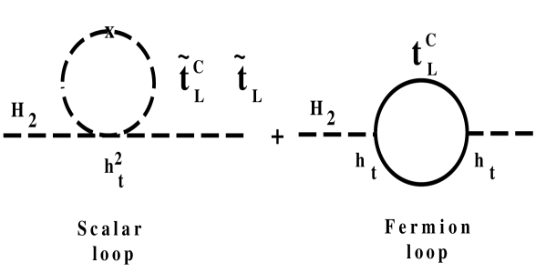
Figure 4.5: Corrections to the Higgs self-energy from Yukawa type interactions.

4.7 Electroweak Symmetry Breaking

The coupling $\mu$ plays an important role in the shape of the potential and consequently in the pattern of electroweak symmetry breaking, which occurs if the minimum of the potential is not obtained for $<H_{1}>$=$<H_{2}>$=0. In the SM this condition could be introduced ad-hoc by requiring the coefficient of the quadratic term to be negative. In supersymmetry this term is restricted by the gauge couplings[34]. A non-trivial minimum can only be obtained by the soft breaking terms, if the mass matrix for the Higgs sector, given by $M_{ij}^{2}=\frac{\partial^{2}V}{\partial H_{i}\partial H_{j}}$, has a negative eigenvalue. This is obtained if the determinant is negative, i.e.

$$|m_{3}^{2}(t)|^{2}>m_{1}^{2}(t)~{}m_{2}^{2}(t).$$ (4.50)

In order that the new minimum is below the trivial minimum with $<H_{1}>$=$<H_{2}>$=0, one has to require in addition $V_{H}(v_{1},v_{2})<V_{H}(0,0)<V_{H}(\infty,\infty)$, which is fulfilled if

$$m_{1}^{2}(t)+m_{2}^{2}(t)\geq 2|m_{3}^{2}(t)|.$$ (4.51)

If one compares eqns. 4.50 and 4.51 and notices from eq. 4.39 that $m_{1}=m_{2}$, one realizes that these conditions cannot be fulfilled simultaneously, at least not at the GUT scale.

However, at lower energies there are substantial radiative corrections, which can cause differences between $m_{2}$ and $m_{1}$, since the first one involves mass corrections proportional to the top Yukawa coupling $Y_{t}(0)$, while for the latter these corrections are proportional to the bottom Yukawa coupling. Typical diagrams are shown in fig. 4.5. From the RGE for the mass parameters in the Higgs potential one finds at the weak scale:

$$\mu^{2}(t=66) = 0.40\mu^{2}(0)$$ (4.52)

$$m_{1}^{2}(t=66) = m_{0}^{2}+0.40\mu^{2}(0)+0.52m^{2}_{1/2}$$ (4.53)

$$m^{2}_{2}(t=66) = -0.44m_{0}^{2}+0.40\mu^{2}(0)-3.11m^{2}_{1/2}$$ (4.54)

$$-0.09A_{t}(0)m_{0}m_{1/2}-0.02A_{t}(0)^{2}m_{0}^{2}$$

$$m^{2}_{3}(t=66) = 0.63m^{2}_{3}(0)+0.04\mu(0)m_{1/2}+0.19A_{t}(0)m_{0}\mu(0).$$ (4.55)

The coefficients were evaluated for the parameters of the fit to the experimental data (central column of table 6.1 in chapter 6). The explicit dependence of the coefficients on the coupling constants is given in the appendix. The coefficients of the last three terms in $m_{2}$ depend on the top Yukawa coupling. This dependence disappears if the masses of the stop and top quarks in the diagrams of fig. 4.5 are equal. However, if the stop mass is heavier, the negative contribution of the diagram with the top quarks dominates; in this case $m_{2}$ decreases much faster than $m_{1}$ with decreasing energy and the potential takes the form of a mexican hat, as soon as conditions 4.50 and 4.51 are satisfied. Since $A(t)$ is expected to be small, the dominant negative contribution is proportional to $m_{1/2}$ (see eq. 4.54), so the electroweak breaking scale is a sensitive function of both the initial conditions, the top Yukawa coupling and the gaugino masses.

The minimum of the potential can be found by requiring:

$$\frac{\partial V}{\partial|H_{1}^{0}|} = 2m_{1}^{2}v_{1}-2m_{3}^{2}v_{2}+\frac{g^{2}+g^{{}^{\prime}2}}{2}(v_{1}^{2}-v_{2}^{2})v_{1}=0$$

$$\frac{\partial V}{\partial|H_{2}^{0}|} = 2m_{2}^{2}v_{2}-2m_{3}^{2}v_{1}-\frac{g^{2}+g^{{}^{\prime}2}}{2}(v_{1}^{2}-v_{2}^{2})v_{2}=0$$

Here we substituted

$$<H_{1}>\equiv v_{1}=v\cos\beta,\ \ <H_{2}>\equiv v_{2}=v\sin\beta,$$

where

$$v^{2}=v_{1}^{2}+v_{2}^{2}~{}~{}(v\approx 174~{}{\rm GeV}),\ \ \tan\beta\equiv\frac{v_{2}}{v_{1}}.$$

From the minimization conditions given above one can derive easily:

$$v^{2} = \frac{\displaystyle 4}{\displaystyle(g^{2}+g^{{}^{\prime}2})(\tan^{2}\beta-1)}\left\{m_{1}^{2}-m_{2}^{2}\tan^{2}\beta\right\}$$ (4.56)

$$2m_{3}^{2} = (m_{1}^{2}+m_{2}^{2})\sin 2\beta$$ (4.57)

$$M^{2}_{Z}\equiv\frac{g^{2}+g^{{}^{\prime}2}}{2}v^{2} = 2\frac{\displaystyle m^{2}_{1}-m^{2}_{2}\tan^{2}\beta}{\tan^{2}\beta-1}$$ (4.58)

$$M^{2}_{W}\equiv\frac{g^{2}}{2}v^{2} = M_{Z}^{2}{\;\cos^{2}\theta_{W}}$$ (4.59)

The derivation of these formulae including the one-loop radiative corrections is given in the appendix.

Chapter 5 The Big Bang Theory

5.1 Introduction

In the 1920’s Hubble discovered that most galaxies showed a redshift in the visible spectra, implying that they were moving away from each other. This observation is one of the basic building blocks of the Big Bang Theory[4], which assumes the universe is expanding, thus solving the problem that a static universe cannot be stable according the Einstein’s equations of general relativity.

Figure 5.1: Spectrum of the microwave background radiation as measured by the COBE satellite. The curve is the black body radiation corresponding to a temperature of $2.726$ K.

Figure 5.2: Big Bang nucleosynthesis predictions for the primordial abundance of the light elements as function of the primordial ratio $\eta$ of baryons and photons. From ref. [49].

An expanding universe will cool down, so at the beginning the universe might have been hot. The remnants of the radiation of such a hot universe can still be observed today as microwave background radiation corresponding to a temperature of a few degrees. This radiation was first predicted by Gamow, but accidentally observed in 1963 by Penzia and Wilson from Bell Laboratories as noise in microwave antennas used for communication with early satellites. Such an antenna is only sensitive to a single frequency. Recently, the whole spectrum was measured by the COBE satellite and it was found to be indeed describable by a black body radiation, as shown in fig. 5.1 (from ref. [1]). The deviation from perfect isotropy, if one ignores the dipole anisotropy from the Doppler shift caused by the movement of the earth through the microwave background, is a few times $10^{-6}$. This has strong implications for theories concerning the clustering of galaxies, since this radiation was released soon after the “bang” and hardly interacted afterwards, so the inhomogeneities in this radiation are proportional to the density fluctuations in the early universe! These density fluctuations are the seeds for the final formation of galaxies. As will be discussed later, such small anisotropies have strong implications for the models trying to understand the formation of galaxies and the nature of the dark matter in the universe. Direct evidence that the temperature from the microwave background is indeed the temperature of the universe came from the measurement of the temperature of gas clouds deep in space. As it happens, the rotational energy levels of cyanogen $(CN)$ are such that the 3K background radiation can excite these molecules. From the detection of the relative population of the groundstate and the higher levels the excitation temperature was determined to be $T_{CN}=2.729^{+0.023}_{-0.031}$ K[50], which is in excellent agreement with the direct measurement of the microwave background of $2.726\pm 0.010$ K by COBE[51].

Other evidence that the universe was indeed very hot at the beginning came from the measurement of the natural abundance of the light elements: the universe consists for 74% out of hydrogen, 24% helium and 1% for the remaining elements. Both the rarity of heavy elements and the large abundance of helium are hard to explain, unless one assumes a hot universe at the beginning.

The reason for the low abundance of the heavier elements in a hot universe is simple: they are cracked by the intense radiation around. The abundance of the light elements is plotted in fig. 5.2 as function of the ratio $\eta$ of primordial baryons and photons (from ref. [49]). Agreement with experimental observations can only be obtained for $\eta$ in the range $3-7\cdot 10^{-10}$.

The very heavy elements can be produced only at much lower temperatures, but high pressure, so it is usually assumed that the heavy elements on earth and in our bodies were cooked by the high pressure inside the cores of collapsing stars, which exploded as supernovae and put large quantities of these elements into the heavens. They clustered into galaxies under the influence of gravity.

Figure 5.3: The $Z^{0}$ lineshape for different number of neutrino types. The data (black points) exclude more than three types with mass below $M_{Z}/2\approx 45$ GeV.

The ratio of helium and hydrogen is determined by the number of neutrons available for fusion into deuterium and subsequently into helium at the freeze-out temperature of about 1 MeV or $10^{10}$ K. At these high temperatures no complex nuclei can exist, only free protons and neutrons. They can be converted into each other via charged weak interactions like $ep\leftrightarrow\nu_{e}n$ and $\overline{e}n\leftrightarrow\overline{\nu}_{e}p$. Note that this is the same interaction which is responsible for the decay of a free neutron into a proton, electron and antineutrino. The weak interactions maintain thermal equilibrium between the protons and neutrons as long as the density and temperature are high enough, thus leading to a Boltzmann distribution:

$$\frac{n}{p}=e^{-Q/kT},$$ (5.1)

where $Q=(m_{n}-m_{p})c^{2}=1.29$ MeV is the energy difference between the states. Thermal equilibrium is not guaranteed anymore if the weak interaction rates $\Gamma$ are slower than the expansion rate of the universe given by the Hubble constant, i.e. freeze-out occurs when $\Gamma<H(t)$. This happens by the time the temperature is about $10^{9}$ K or 0.1 MeV. Then the ratio $n/p$ is about 1/7. Since the photon energies at these temperatures are too low to crack the heavier nuclei, nuclei can form through reactions like $n+p\leftrightarrow^{2}H+\gamma$, ${}^{2}H+p\leftrightarrow^{3}H+\gamma$ and ${}^{2}H+n\leftrightarrow^{3}H+\gamma$, which in turn react to form ${}^{4}He$. The latter is a very stable nucleus, which hardly can be cracked, so the chain essentially stops till all neutrons are bound inside ${}^{4}He$! Heavier nuclei are hardly produced at this stage, since there are no stable elements with 5 or 8 nuclei, so as soon as ${}^{4}He$ catches another nuclei it will decay. Consequently the $n/p$ ratio 1/7, as determined from the Boltzmann distribution, yields a ${}^{4}He$ mass fraction $Y_{He}$

$$Y_{he}=\frac{2n/p}{n/p+1}\approx\frac{1}{4}.$$ (5.2)

Experimentally the mass fraction $Y_{P}$ of ${}^{4}He$ is $23\pm 1\%$ [52]! The mass fractions of deuterium, ${}^{3}He$, and ${}^{7}Li$ are many orders of magnitude smaller[1, 2]. The concentration of the latter elements is a strong function of the primordial baryon density (see fig. 5.2), since at high enough density all the deuterium will fuse into ${}^{4}He$, thus eliminating the “components” for ${}^{3}He$ and ${}^{7}Li$.

As said above, freeze-out occurs, if $\Gamma<H(t)$. Thus the expansion rate $H(t)$ around $T\approx 1$ MeV determines the ${}^{4}He$ abundance. The expansion rate in turn is determined by the fraction of relativistic particles, like neutrinos, light photinos etc. Roughly for each additional species the primordial ${}^{4}He$ abundance increases by 1%, as shown in fig. 5.2 for a neutron half-life time of 10.6 minutes (from ref. [49]). The neutron lifetime is not negligible on the scale of the first three minutes, so it has to be taken into account. If one wants to reconcile the abundance of all light elements, there can only be three neutrino species (see fig. 5.2) with practically no room for other weakly interacting relativistic particles like light photinos! Present collider data confirm that there are indeed only three light neutrinos[30]:

$$N_{\nu}=2.99\pm 0.04.$$ (5.3)

The strongest constraint comes from the $Z^{0}$ resonance data at LEP[54]. An example of the quality of the data is shown in fig. 5.3. Note that collider data limit the number of neutrino generations, while nucleosynthesis is sensitive to all kinds of light particles, where light means about one MeV or less. Happily enough the collider data require the lightest neutralino to be above 18.4 GeV[30], so there is no conflict between cosmology and supersymmetry.

Note that this is a beautiful example of the interactions between cosmology and elementary particle physics: from the Big Bang Theory the number of relativistic neutrinos is restricted to three (or four if one takes the more conservative upper limit on the ${}^{4}He$ abundance to be 0.25) and at the LEP accelerator one observes that the number of light neutrinos is indeed three! Alternatively, one can combine the accelerator data and the abundance of the light elements to “postdict” the primordial helium abundance to be 24% and use it to obtain an upper limit on the baryonic density[52]:

$$\rho_{b}\leq 0.1\rho_{c},$$ (5.4)

where $\rho_{c}$ is the critical density needed for a flat universe. The critical density will be calculated in section 5.4. Thus LEP data in combination with baryogenesis strengthens the argument that we need non-baryonic dark matter in a flat universe, for which $\rho=\rho_{c}$. Other arguments for dark matter will be discussed in section 5.12.

In spite of the marvelous successes of this model of the universe, many questions and problems remain, as mentioned in the Introduction. However, GUT’s can provide amazingly simple solutions, at least in principle, since many details are still open.

These problems will be discussed more quantitatively in the next sections, starting with Einsteins equations in a homogeneous and isotropic universe, conditions which have been well verified in the present universe and which make the solutions to Einstein’s equations particularly simple. Especially, it is easy to see that a phase transition can lead to inflation, the key in all present cosmological theories.

5.2 Predictions from General Relativity

At large distances the universe is homogeneous, i.e. one finds the same mass density everywhere in the universe, typically

$$\rho_{univ}=(4-16)~{}10^{-27}~{}{\rm kg/m^{3}},$$ (5.5)

which corresponds to 2.5 -10 hydrogen atoms per cubic meter. (In comparison, an extremely good vacuum of $10^{-9}N/m^{2}$ at 300 K contains about $2~{}10^{11}$ molecules per cubic meter. Of course, the volume to be averaged over should be chosen to be much larger than the size of clusters of galaxies. Furthermore, the same density and temperature is observed in all directions, i.e. the universe is very isotropic. If no point and no direction is preferred in the universe, the possible geometry of the universe becomes very simple: the curvature has to be the same everywhere, i.e. instead of a curvature tensor one needs only a single number, usually written as $K(t)=k/R^{2}(t)$, where $R(t)$ is the so-called scale factor. This factor can be used to define dimensionless time-independent (comoving) coordinates in an expanding universe: the proper (or real) distance $D(t)$ between two galaxies scales as

$$D(t)=R(t)d,$$ (5.6)

where $d$ is the distance at a given time $t_{0}$. The factor $k$ introduced above defines the sign of the curvature: $k=0$ implies no curvature, i.e. a flat universe, while $k=+1(-1)$ corresponds to a space with a positive curvature (spherical) and $k=-1$ corresponds to a space with a negative curvature (hyperbolic).

The movement of a galaxy in a homogeneous universe can be compared to the molecules in a gas; the stars are just the atoms of a molecule and the molecules are homogeneously distributed. Differentiating equation 5.6 results in

$$v=\dot{R}(t)d,$$ (5.7)

or substituting $d$ from eq. 5.6 results in the famous relation between the velocity and the distance of two galaxies:

$$v=\frac{\dot{R}(t)}{R(t)}D(t)\equiv H(t)D(t),$$ (5.8)

where $H(t)$ is the famous Hubble constant.

This relation between the velocity and the distance of the galaxies was first observed experimentally by Hubble in the 1920’s. He observed that all neighbouring galaxies showed a redshift in the spectral lines of the light emitted by specific elements and the redshift was roughly proportional to the distance. So this was the first evidence that we are living in an expanding universe, which might have been created by a “Big Bang”.

The Hubble relation 5.8 is a direct consequence of the homogeneity and isotropy of the universe, since the scale factor cannot be a constant in that case. This follows directly from Einstein’s field equations of general relativity, which can be written as:

$$\ddot{R}(t) = -\frac{4\pi~{}G}{3c^{2}}(u(t)+3p(t))R(t),$$ (5.9)

$$\frac{\dot{R}(t)^{2}}{R^{2}(t)}-\frac{8\pi~{}G}{3c^{2}}u(t) = -\frac{kc^{2}}{R^{2}},$$ (5.10)

where $G=6.67\cdot 10^{-11}{\rm Nm^{2}/kg^{2}}$ is the gravitational constant, $\dot{R}$ and $\ddot{R}$ are the derivatives of $R$ with respect to time, $p$ is the pressure and $u$ is the energy density.

A static universe, in which the derivatives and pressure are zero, implies $u(t)=0$, so a static universe cannot exist unless one introduces additional potential energy in the universe, e.g. Einstein’s cosmological constant. At present there is no experimental evidence for such a term[43].

5.3 Interpretation in terms of Newtonian Mechanics

Since the energy density, and correspondingly the curvature, is small in our present universe, relativistic effects can be neglected and the field equations 5.9 and 5.10 have a simple interpretation in terms of Newtonian mechanics. Consider a spherical shell with radius R and mass $m$. The mass inside this sphere can be related the average density $\rho$:

$$M=\frac{4}{3}\pi R^{3}\rho.$$ (5.11)

For an expanding universe the total mechanical energy of the mass shell can be written as the sum of the kinetic and potential energy:

$$E_{tot} = \frac{1}{2}m\dot{R}^{2}-\frac{GMm}{R}$$ (5.12)

$$= \frac{1}{2}mR^{2}\left[\frac{\dot{R}^{2}}{R^{2}}-\frac{8}{3}\pi G\rho\right].$$

The expression in brackets is just the left hand side of eq. 5.10, so the sum of kinetic – and potential energy determines the sign of the curvature $k$. If $k=1$, then $E_{tot}<0$, implying that the universe will recollapse under the influence of gravity (“Big Crunch”), just like a rocket which is launched with a speed below the escape velocity, will return to the earth; $k=-1$, on the other hand, implies that the universe will expand and cool forever (“Big Chill”). In case of $k=0$ the total energy equals zero (flat Euclidean space), in which case the gravitational energy, or equivalently the mass density, is sufficient to halt the expansion.

The first field equation (eq. 5.9) follows from the second equation (eq. 5.10) by differentiation and taking into account that in an expanding universe energy is converted into gravitational potential energy: when the volume increases by an infinitesimal amount $\Delta V$, then the remaining energy in the gas decreases by an amount $p\Delta V_{phys}$, where $p$ denotes the pressure. Therefore

$$\dot{E}(t)=-p(t)\dot{V}_{phys}(t)=-3\frac{\dot{R}(t)}{R(t)}p(t)V_{phys}(t).$$ (5.13)

Here we used $V_{phys}=V_{0}R^{3}(t)$, where $V_{0}$ is the volume in comoving time-independent coordinates analogous to eq. 5.6. On the other hand follows from $E(t)=u(t)V_{phys}(t)$

$$\dot{E}(t)=\dot{u(t)}V_{phys}(t)+3\frac{\dot{R}(t)}{R(t)}u(t)V_{phys}(t).$$ (5.14)

Combining eqs. 5.13 and 5.14 results in:

$$\dot{u}(t)=-3\frac{\dot{R}(t)}{R(t)}(u(t)+p(t)).$$ (5.15)

Substituting this equation for $\dot{u}(t)$ after differentiation of eq. 5.10 yields eq. 5.9.

5.4 Time Evolution of the Universe

To find out how the universe will evolve in time, one needs to know the equation of state, which relates the energy density to pressure. Usually energy and pressure are proportional, i.e. $p=\alpha\rho c^{2}$, where $\alpha=0$ for cold non-relativistic matter ($p=0)$ and $\alpha=1/3$ for a relativistic hot gas, as follows from elementary Thermodynamics. From eq. 5.15 given above, it follows immediately that

$$\rho\propto R^{-3(1+\alpha)}$$ (5.16)

and substituting this into eq. 5.10 results in:

$$R\propto t^{\frac{2}{3(1+\alpha)}},$$ (5.17)

if we neglect the curvature term, i.e. either $R$ is large or $k$ small. As we will see, both are true after the inflationary phase of the universe.

$\begin{array}[]{|c|c|c|c|}\hline\cr hot~{}relativistic&t>t_{1}&R\propto t^{1/2}&\rho=D_{1}/R^{4}\\ \hline\cr inflation&t_{1}>t>t_{2}&R\propto e^{Ht}&\rho=const.\\ \hline\cr hot~{}relativistic&t_{2}>t>t_{3}&R\propto t^{1/2}&\rho=D_{2}/R^{4}\\ \hline\cr cold~{}non-relativ.&t>t_{3}&R\propto t^{2/3}&\rho=D_{3}/R^{3}\\ \hline\cr\end{array}$

Table 5.1: The time dependence of the scale factor and energy density during various stages in the evolution of the universe. Typically, $t_{1}\approx 10^{-43}$ s, $t_{2}\approx 10^{-35}$ s, and $t_{3}\approx 10^{5}$ yrs. The constants $D_{i}$ are integration constants.

The time dependence has been summarized in table 5.1 for various stages of the universe. The inflationary period will be discussed in the next section. One observes that the scale factor vanishes at some time $t=0$ and the energy density becomes infinite at that time. This singularity explains the popular name “Big Bang” theory for the evolution of the universe. The solutions for $R(t)$ are shown graphically in fig. 5.4 for three cases: a flat universe ($k=0$), an open universe ($k=-1$) and a closed universe ($k=1$) (from ref.[3]).

Figure 5.4: Evolution of the radius of the universe for a closed (C), flat (F) or open (O) universe with and without inflation. From ref. [3].

An open or flat universe will expand forever, since the kinetic energy is larger than the gravitational attraction. A closed universe will recollapse. The lifetime of a closed universe with $p>-\rho/3$ and a total mass M of cold non-relativistic matter is[3]:

$$t_{c}=\frac{4MG}{3}\approx\frac{M}{M_{P}}~{}10^{-43}s,$$ (5.18)

so the present lifetime of the universe of at least $10^{10}$ yrs gives a strong upper limit on the density of the universe.

The lifetime can easily be calculated, if we assume a flat universe: from table 5.1 it follows that $R(t)\propto t^{2/3}$ for most of the time. Substituting this and its time derivative into the definition of the Hubble constant (eq. 5.8 ) results in:

$$H(t)=\frac{2}{3t}.$$ (5.19)

With the presently accepted value of the measured Hubble constant:

$$H=100~{}h_{0}~{}(\frac{km}{s~{}Mpc})\approx h_{0}~{}(3~{}10^{17})^{-1}s^{-1}\approx h_{0}~{}10^{-10}~{}yrs^{-1},$$ (5.20)

where $h$ indicates the experimental uncertainty ($0.4\leq h_{0}\leq 1$), one finds for the age of the universe:

$$t_{universe}=2/3H=2/(3h_{0})\cdot 10^{10}{\rm yrs}.$$ (5.21)

The critical density, which is the density corresponding to a flat universe, can be calculated from eqn. 5.12 by requiring $E_{tot}=0$ (or equivalently $k=0$) and substituting for $\dot{R}/R$ the Hubble constant (see eq. 5.8):

$$\rho_{c}=\frac{3H^{2}}{8\pi G}=2\cdot 10^{-26}~{}h_{0}^{2}~{}kg/m^{3},$$ (5.22)

where the numerical value of $H$ from eq. 5.20 was used.

The size of the observable universe, the horizon distance $D_{h}$, can be calculated in the following way: the proper distance between two points is $R(t)d$ (eq. 5.6), where $d$ is the distance in comoving coordinates. Light propagates on the light-cone. This can be studied most easily by considering the time $\eta$ in comoving coordinates with

$$dt=R(t)d\eta.$$ (5.23)

In comoving coordinates the distance $d_{h}$ light can propagate is $cd\eta$, so $d_{h}\equiv c\int d\eta=c\int dt/R(t)$ or the proper distance $D_{h}=R(t)d_{h}$ equals:

$$D_{h}=cR(t)\int_{0}^{t^{\prime}}\frac{dt^{\prime}}{R(t^{\prime})}.$$ (5.24)

For most of the time $R(t)=at^{2/3}$ (see table 5.1). Substituting this into eq. 5.24 yields:

$$D_{h}=3ct=2c/H(t)=0.9h_{0}^{-1}\cdot 10^{26}~{}{\rm m},$$ (5.25)

where for the lifetime $t$ of the universe eqs. 5.19 and 5.20 were used.

5.5 Temperature Evolution of the Universe

In the previous section the scale factor and the energy density were calculated as function of time. The energy density has two components: the energy density from the photon radiation in the microwave background $\rho_{rad}$ and the energy density of the non-relativistic matter $\rho_{matter}.$ At present $\rho_{rad}$ is negligible, but at the beginning of the universe it was the dominating energy. Assuming this radiation to be in thermal equilibrium with matter implies a black body radiation with a frequency distribution given by Planck’s law and an energy density

$$\rho_{rad}=aT^{4},$$ (5.26)

where $a=7.57\cdot 10^{-16}~{}J~{}m^{-3}K^{-4}.$ Since $\rho_{rad}\propto 1/R^{4}$ (see table 5.1) one finds from eq. 5.26:

$$T\propto 1/R(t),$$ (5.27)

from which follows immediately: $\dot{R}/R=-\dot{T}/T$ and $R^{-2}\propto T^{2}$. Substituting these expressions and eq. 5.26 into the second field equation (eq. 5.10) leads to:

$$\left(\frac{\dot{T}}{T}\right)^{2}=\frac{8\pi aG}{3c^{2}}T^{4},$$ (5.28)

since the term with $kc^{2}$ is only proportional to $T^{2}$, so it can be neglected at high temperatures. Integrating eq. 5.28 yields:

$$T=\left(\frac{3c^{2}}{32\pi aG}\right)^{1/4}\cdot\frac{1}{\sqrt{t}}=1.5\cdot 10^{10}~{}K\cdot\sqrt{\frac{1~{}s}{t}}=1.3~{}MeV\sqrt{\frac{1~{}s}{t}},$$ (5.29)

so the temperature drops as $1/\sqrt{t}.$

From this equation one observes that about one microsecond after the Big Bang the temperature has dropped from a value above the Planck temperature, corresponding to an energy of $10^{19}$ GeV to a temperature of about one GeV, so after about one microsecond the temperature is already too low to generate protons and after about one second the lightest matter particles, the electrons, are “frozen” out. After about three minutes the temperature is so low that the light elements become stable, and after about $10^{5}$ years atoms can form.

At this moment all matter becomes neutral and the photons can escape. These are the photons, which are still around in the form of the microwave background radiation!

Figure 5.5: The flatness of the universe after inflation is easily understood if one thinks about the inflation of a balloon.

Figure 5.6: The space-time diagram of the microwave background radiation, which was released at the time $t_{r}$. Photons observed in point P from opposite directions traveled some $10^{10}$ yrs with hardly any interactions from the points A and B, respectively. The distance light could have traveled between the Big Bang and $t_{r}$ is only $ab$, which is much smaller than the distance $AB$. Consequently the points A and B could never have been in causal contact with each other. Nevertheless, the radiation from A and B have the $same$ temperature, although the horizon $ab$ is much smaller (horizon problem). The problem can be solved if one assumes the region of causal contact was much larger than $ab$ through inflation of space-time via a phase transition.

After the discovery of the microwave background radiation, the Big Bang theory gained widespread acceptance. Nevertheless, the simplest model as formulated here, has several serious problems, which can only be solved by the so-called inflationary models. These models have the bizarre property that the expansion of the universe goes faster than the speed of light! This is not a contradiction of special relativity, since these regions are causally disconnected, so no information will be transmitted. Special relativity does not restrict the velocities of causally disconnected objects. However, such inflationary scenarios require the introduction of a scalar field, e.g. the Higgs field discussed in the previous chapter. For certain conditions of the potential of this field, the gravitational force becomes repulsive, as can be derived directly from the Einstein equations given above. This will be discussed in more detail after a short summary of the main problems and questions of the simple Big Bang theory.

5.6 Flatness Problem

At present we do not know if the universe is open or closed, but experimentally the ratio of the actual density to the critical density is bound as follows[2]:

$$0.1\leq\Omega=\rho/\rho_{c}\leq 2.$$ (5.30)

The luminous matter contributes only about 1% to $\Omega$, but from the dynamics of the galaxies one estimates that the galaxies contribute between 0.1 and 0.3, so the lower limit on $\Omega$ stems from these observations. The upper limit is obtained from the lower limit on the lifetime of the universe. From the dating of the oldest stars and the elements one knows that the universe is at least $10^{10}$ years old, which gives an upper limit on the Hubble constant (eq. 5.19) and consequently on the density[2]. This does look like a perfectly acceptable number and the universe might even be perfectly flat, since $\Omega=1$ is not excluded. However, it can be shown easily, that $\Omega-1$ grows with time as $t^{2/3}$ and for the present lifetime $t\approx 10^{17}s$ this number becomes big, unless very special initial conditions limit the proportionality constant to be exceedingly small. This constant can be calculated easily: From eq. 5.10 and the definition of $\rho_{c}$ (eq. 5.22) one finds:

$$\Omega(t)-1=\frac{kc^{2}}{R^{2}(t)H^{2}(t)}$$ (5.31)

Since $R\propto t^{2/3}$ for the longest time of the universe (see table 5.1) and $H(t)\propto 1/t$ (eq. 5.21) one observes that $\Omega-1\propto kt^{2/3}$. For this number to come out close to zero for $t$ very large implies that $k$ must have been very close to zero, right from the beginning. Remember that $k$ is proportional to the sum of potential and kinetic energy in the non-relativistic approximation. One can show[3] that in order for $\Omega$ to lie in the range close to 1 now, implies that in the early universe $|\Omega-1|\leq 10^{-59}M_{P}^{2}/T^{2}$, or for $T\approx M_{P}$,

$$\frac{|\Omega-1|}{\Omega}\leq 10^{-59}.$$ (5.32)

In other words, if the density of the initial universe was above the critical density say by $10^{-55}\rho_{c}$, the universe would have collapsed long ago! On the other hand, would the density have been below the critical density by a similar amount, the present density in the universe would have been negligible small and life could not exist!

5.7 Horizon Problem

Since the horizon increases linearly with time but the expansion only with $t^{2/3}$, most of the presently visible universe was causally disconnected at the time $t=10^{5}$ years, when the microwave background was released. Nevertheless, the temperature of the microwave background radiation is the same in all directions! How did these photons thermalize after being emitted some $10^{10}$ years ago? One should realize that the density in the universe is exceedingly low, so photons from opposite directions have traveled some $2\cdot 10^{10}$ lightyears without interactions. Since the distance scales as $t^{2/3}$, these regions were about $10^{7}$ light years apart at the time they were released, i.e. the distance $AB$ in fig. 5.6, which is two orders of magnitude larger than the horizon of the universe at that time (distance $ab$), so no signal could have been transmitted. Nevertheless, the temperature difference $\Delta T/T$ between these regions is less than $10^{-5}$ as shown by the recent COBE data. As with the flatness problem, one can impose an accidental temperature isotropy in the universe as an initial condition, but with all the hefty fluctuations during the Big Bang, this is a very unsatisfactory explanation. As we will see later, inflation solves both problems in a very elegant way.

5.8 Magnetic Monopole Problem

Magnetic monopoles are predicted by GUT’s as topological defects in the Higgs field: after spontaneous symmetry breaking the vacuum obtains a non-zero vacuum expectation value in a given region. Different regions may have different orientations of the phases of the Higgs field and the borderlines of these regions have the properties expected for magnetic monopoles[55]. Unfortunately the magnetic monopole density is very small, if not zero. Their absence has to be explained in any theory based on GUT’s with SSB. The first attack was made by Alan Guth, who invented inflation for this problem. Although the original model did not solve the monopole problem, it provided a perfectly reasonable solution for the horizon and flatness problem. An alternative version of inflation, the so-called new inflation, which was invented by A.D. Linde[3] and independently by Albrecht and Steinhardt[56], provided also a solution of the monopole problem, as will be discussed in section 5.10.

5.9 The smoothness Problem

Our universe has density inhomogeneities in the form of galaxies. On a large scale the spectrum of inhomogeneities is approximately scale-invariant, which can be understood in the inflationary scenario as follows: the inflation smoothens out any inhomogeneities which might have been present in the initial conditions. Then in the course of the phase transition inhomogeneities are generated by the quantum fluctuations of the Higgs field on a very small scale of length, namely the scale where quantum effects are important. These density fluctuations are then enlarged to an astronomical scale by inflation and they stay scale invariant as is obvious if one thinks about a little circle on a balloon, which stays a circle after inflation, but just on a larger scale.

5.10 Inflation

The deceleration in the universe is given by eq. 5.9. In case the energy density only consists of kinetic and gravitational energy, the sign of $\ddot{R}$ is negative, since both the pressure and energy density are positive. However, the situation can change drastically, if the universe undergoes a first-order phase transition. In Grand Unified Theories such phase transitions are expected: e.g. the highly symmetric phase might have been an SU(5) symmetric state, while the less symmetric state corresponds to the ${SU(3)_{C}\otimes\-SU(2)_{L}\otimes\-U(1)_{Y}}$ symmetry of the Standard Model. The description of the spontaneous symmetry breaking by the Higgs mechanism leads to a specific picture of this phase-transition: the Higgs field $\phi$ is a scalar field, which fills the vacuum with a potential energy $V(\phi)$. The value of the potential is temperature dependent: at high temperatures the minimum occurs for $\phi=0$, but for temperatures below the critical temperature, the ground state, i.e. the state with the lowest energy, is reached for a value of the field $\phi\neq 0$. This is completely analogous to other phase transitions, e.g. in superconductivity the scalar field corresponds to the density of spin 0 Cooper pairs or in ferromagnetism it would be the magnetization.

If during the expansion of the universe the energy density falls below the energy density of this scalar field, something dramatic can happen: the deceleration can become an acceleration, leading to a rapid expansion of the universe, usually called “inflation”.

This can be understood as follows: if the vacuum is filled with this potential energy of the scalar field with an energy density $\rho_{vac}$, the work $W$ done during the expansion is $p\Delta V$. However, the gain in energy is $\rho_{vac}\Delta V$, since the potential energy of the vacuum does not change (a “void” stays a “void” as long as no phase transition takes place), so an increase in volume implies an increase in energy. Since no external energy is supplied, the total energy of the system must stay constant, i.e. $p\Delta V+\rho_{vac}\Delta V=0,$ or

$$p=-\rho_{vac}.$$ (5.33)

This is the famous equation of state in case of a potential dominated vacuum. In this case eq. 5.10 reduces to:

$$\ddot{R}=\frac{8}{3}\pi GR(t){\rho}.$$ (5.34)

This equation has the solution:

$$R(t)\propto e^{t/\tau},$$ (5.35)

where

$$\tau=\sqrt{\frac{3}{8\pi G\rho}}.$$ (5.36)

As we have seen in the previous chapter, the symmetry breaking of a GUT happens at an energy of $10^{16}$ GeV. The energy density at this energy is extremely high:

$$u=\rho c^{2}=\frac{E^{4}_{GUT}}{(\hbar c)^{3}}=10^{100}~{}{\rm Jm^{-3}},$$ (5.37)

where the powers are derived from dimensional analysis. Inserting this result into eq. 5.36 yields:

$$\tau=10^{-37}s.$$ (5.38)

Thus the universe inflates extremely rapidly: its diameter doubles every $\tau\ln 2$ s! The behaviour of the Hubble constant during the inflationary era is then determined by eq. 5.8, which yields:

$$H(t)=\frac{1}{\tau}.$$ (5.39)

Clearly, the inflationary scenario provides in an elegant way solutions for many of the shortcomings of the BBT:

• The rapid expansion removes all curvature in space-time, thus providing a solution for the flatness problem.

• After expansion the universe reheats because of the quantum fluctuations around the new minimum of the vacuum, thus thermalizing a region much larger than the visible region at that time. This explains why all visible regions in the present universe were in causal contact during the time the 2.7 K background microwave radiation was released.

• The rapid expansion explains the absence of magnetic monopoles, since after sufficiently large inflation the monopoles are diluted to a negligible level.

However, the whole idea of inflation only works if one assumes the inflation to go smoothly from a single homogenous region to a large homogenous region many times the size of our universe (so-called new inflation). This requires rather special conditions for the shape of the potential, as was pointed out by Linde[3] and independently by Albrecht and Steinhardt[56] after the original introduction of inflation by Guth[56]. The problem is that the corresponding scalar fields providing the potential energy of the vacuum have to be weakly interacting, since otherwise the phase transition will involve only microscopic distances according to the uncertainty relation. The Higgs fields providing spontaneous symmetry breaking are interacting too strongly, so one has to introduce additional weakly interacting scalar fields. It is non-trivial to combine the requirement of a negligible small cosmological constant, which represents the potential energy of the vacuum, with a vacuum filled with Higgs fields to generate masses. This requires large cancellations of positive and negative contributions, which occur e.g. in unbroken supersymmetric theories. However, these theories, if they describe the real world, have to be broken. Details on these problems are discussed by Olive[49] and in the recent text books by Börner[1] and Kolb and Turner[2]. In spite of these problems the arguments in favour of inflation are so strong, that it has become the only acceptable paradigm of present cosmology.

5.11 Origin of Matter

As discussed above, matter in our universe consists largely of hydrogen (75%) and helium (24%) (typically $10^{78}$ nucleons). The absence of antimatter can be explained if one has phase transitions and among others CP-violation, as discussed in chapter 3. At present the nuclei dominate the energy density in the universe in contrast to the first $10^{5}$ years, when the energy density of the radiation dominated. The reason for this change is simply the fact that the energy density of the many photons around decreases $\propto T^{4}$, while the energy density of the nuclei decreases $\propto T^{3}$ (see eq. 5.16).

Large amounts of matter can be created from the energy release during the inflationary phase of the universe. This can be easily estimated as follows. After inflation the universe has a macroscopic size, typically the size of a football or larger. The large energy density in this volume (see eq. 5.37) yields a total energy many times the mass in our present universe.

Thus within the inflationary scenario the universe could originate as a quantum fluctuation, starting from absolute “nothing”, i.e. a state devoid of space, time and matter with a total energy equal to zero. Most matter was created after the inflationary phase from the decay of the field quanta of the fields responsable for the inflation. Of course, a quantum description of space-time can be discussed only in the context of quantum gravity, so these ideas must be considered speculative until a theory of quantum gravity is formulated and proven by experiment. Nevertheless, it is fascinating to contemplate that physical laws may determine not only the evolution of our universe, but they may remove also the need for assumptions about the initial conditions.

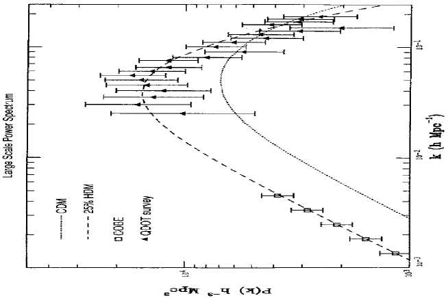
Figure 5.7: Models including 25% hot dark matter (HDM) can describe the large scale structure of the universe, as probed by the galaxy surveys (QDOT) and COBE temperature anisotropy, better than models with only dark matter (DM). From Schaefer and Shafi [57].

5.12 Dark Matter

The visible matter is clustered in large galaxies, which are themselves clustered in clusters and superclusters with immense voids in between. From the movements of the galaxies one is forced to conclude that there must be much more matter than the observed visible matter, if we want to stick to Newtonian mechanics. The most impressive evidence for the dark, i.e. not visible matter comes from the so-called flat rotation curves [58]: the orbital velocities of luminous matter around the central of spiral galaxies remain constant out to the far edges of the galaxies in apparent contradiction to velocity distributions expected from Keppler’s law:

$$v^{2}(r)=G\frac{M(r)}{r},$$ (5.40)

where $r$ is the radial distance to the centre of the galaxy, $M(r)$ the mass of the galaxy inside a sphere with radius $r$, and $G$ the gravitational constant. From this law one expects the velocities to decrease with $1/\sqrt{r}$, if the mass is concentrated in the centre, which is certainly the case for the visible matter. Velocities independent of $r$ imply $M(r)/r$ to be constant or $M(r)\propto r$! Such a behaviour is expected for weakly interacting matter, like neutrinos, gravitinos or photinos, since strongly interacting matter would be attracted to the centre by gravity, interact, loose energy, and concentrate in the centre, just like the visible matter does. Also the dynamical properties of galaxies in large clusters require large amounts of dark matter. To make the speeds work out consistently, one has to assume that the total density of ’dark’ matter is an order of magnitude more than the visible matter. Recent reviews for the experimental evidence of dark matter can be found in ref. [59].

From the concentration of light elements, as shown in fig. 5.2, one has to conclude that the total baryonic density is only about 10% of the critical density (see eq. 5.4). The critical density is the density for a flat universe, which naturally occurs after inflation. Consequently, in the inflationary scenario the dark matter makes up about 90% of the total mass in the universe and it has to be non-baryonic.

Possible candidates for dark matter are the MACHO’s, which have been observed recently through their microlensing effect on the light of stars behind them[60]. But since they cluster in heavy compact objects, they are likely to be remnants of collapsed stars or light dwarfs, which have too little mass to start nuclear burning. In these cases they would be baryonic and make up 10% of the critical density, required by baryogenesis. Note that the visible baryonic matter in stars represents at most 1% of the critical density.

So one needs additional dark matter, if one believes in inflation and takes the value of $\Omega_{b}=0.1$ from baryogenesis. Candidates for this additional dark matter are neutrinos with a mass in the $eV$ range[61]:

$$9<m_{\nu}<35~{}{\rm eV}.$$ (5.41)

Such small masses are experimentally not excluded[30], but they would be relativistic or “hot”. Unfortunately, all dark matter cannot be relativistic, since this is inconsistent with the extremely small anisotropy in the microwave background as observed by the COBE satellite [62].

This anisotropy in the temperature is proportional to the anisotropy in the mass density at the time of release of this radiation shortly after the Big Bang. Through gravity the galaxies were formed around these fluctuations (“seeds”) in the mass density. So the present structure of the universe has to follow from the spectrum of fluctuations in the early universe, which can be probed by the microwave background anisotropy. The best fit is obtained for a mixture of 75% cold and 25% hot dark matter[62], as shown in fig. 5.7 (from ref. [57]).

The lightest supersymmetric particles are ideal candidates for cold dark matter, provided they are not too numerous and too heavy. Otherwise they would provide a density above the critical density[63, 64, 65] in which case the universe would be closed and the lifetime would be very short (see fig. 5.4). The LSP can annihilate sufficiently rapidly into fermion-antifermion pairs, if the masses of the SUSY particles are not too heavy, as will be discussed in chapter 6.

5.13 Summary

The Big Bang theory is remarkably successful in explaining the basic observations of the universe, i.e. the Hubble expansian, the microwave background radiation and the abundance of the elements. From the measured Hubble constant one can derive such basic quantities as the the size and the age of the universe. Nevertheless many questions remain unanswered. They can be answered by postulating phase transitions during the evolution of the universe from the Planck temperature of $10^{32}$ K to the 2.7 K observed today. Among the questions:

• The Matter-Antimatter Asymmetry in our Universe
  As first spelled out by Sakharov[31], any theory trying to explain the preponderance of matter in our universe must necessarily implement:

  • Baryon- and Lepton number violation;

  • C- and CP- violation;

  • Thermal non-equilibrium conditions, as expected after phase transitions.

• The Dominance of Photons over Baryons
  If the excess of matter originates from small CP-violation effects, most matter and antimatter will have enough time to annihilate into photons thus providing an explanation why the number of photons as observed in the 3K microwave background radiation is about $10^{9}$ to $10^{10}$ times as high as the number of baryons in our universe.

• Inflation
  An inflationary phase, i.e. a rapid expansion generated by a potential energy term, which, according to Einstein’s equations of General Relativity, provides a repulsive instead of attractive gravitational force, is the only viable explanation to solve the following problems:

  • Horizon Problem
    The fact that the observed temperature of the 2.7 K microwave background radiation is to a very high degree the same in all directions can only be explained if we assumes that all regions were in causal contact with each other at the beginning. However, the size of our universe is larger than the “horizon”, i.e. the distance light could have traveled since the beginning. Therefore, one can only explain the temperature isotropy, if one assumes that all regions were in causal contact at the beginning and that space expanded faster than the speed of light. This is indeed the case in the inflationary scenario.

  • Flatness Problem
    Experimentally the observed density in our universe is close to the so-called critical density, which is the density, where the total energy of the universe is zero, i.e. the kinetic energy of the expanding universe is just compensated by the gravitational potential energy. This corresponds to a “flat” universe, i.e. zero curvature. The inflationary scenario naturally explains, why the universe is so flat: the rapid expansion by more than 50 orders of magnitude drives all curvature to zero.

  • Magnetic Monopole Problem
    Magnetic monopoles are predicted by GUT’s. Their absence in our universe is explained by the inflationary models, if one assumes the inflation to go smoothly from a single homogeneous region to a large homogeneous region many times the size of our universe (so-called new inflation).

  • The Smoothness Problem
    Experimentally the cosmic background radiation shows the features in accord with the Harrison-Zel’dovich scale-invariant spectrum (n=1)[51], which is the spectrum expected after inflation. The scale invariance can be understood as follows: the inflation smoothens out out any inhomogeneities which might have been present in the initial conditions. Then in the course of the phase transition inhomogeneities are generated by the quantum fluctuations of the Higgs field on a very small scale of length, namely the scale where quantum effects are important. These density fluctuations are then enlarged to an astronomical scale by inflation and they stay scale invariant as is obvious if one thinks about e.g. a little circle on a balloon, which stays a circle after inflation, but just on a larger scale.

In Grand Unified Theories the conditions needed for the inflationary Big Bang Theory are naturally met: at least two phase transitions, which generate mass and thus provide non-equilibrium conditions, are expected: one at the unification scale of $10^{16}$ GeV, i.e. at temperature of about $10^{28}$ K and one at the electroweak scale, i.e. a temperature of about $10^{16}$ K. Furthermore, a potential energy term in the vacuum is expected from the scalar fields in these theories, which are needed to generate particle masses in a gauge-invariant way. In the minimal model at least 29 scalar fields are required. Unfortunately, none have been discovered so far, so little is known about the scalar sector.

Nevertheless, the arguments in favour of inflation are so strong, that it has become the only acceptable paradigm of present cosmology. Experimental observation of scalar fields would provide a great boost in the acceptance of the role of scalar fields, both in cosmology and particle physics.

Chapter 6 Comparison of GUT’s with Experimental Data

In this chapter the various low energy GUT predictions are compared with data. The most restrictive constraints are the coupling constant unification combined with the lower limits on the proton lifetime. They exclude the SM[66, 11, 67] as well as many other models[11, 35, 68] with either a more complicated Higgs sector or models, in which one searches for the minimum number of new particles required to fulfil the constraints mentioned above. From the many models tried, only a few yielded unification at the required energies, but these models have particles introduced ad-hoc without the appealing properties of Supersymmetry. Therefore we will concentrate here on the supersymmetric models and ask if the predictions of the simplest, i.e. minimal models[69] are consistent with all the constraints described in the previous chapters. The relevant RG equations for the running of the couplings and the masses are given in the appendix. Assuming soft symmetry breaking at the GUT scale, all SUSY masses can be expressed in terms of 5 parameters and the masses at low energies are then determined by the well known Renormalization Group (RG) equations. So many parameters cannot be derived from the unification condition alone, However, further constraints can be considered:

• $M_{Z}$ predicted from electroweak symmetry breaking[34, 70, 71, 64, 72].

• b-quark mass predicted from the unification of Yukawa couplings[73, 74, 75].

• Constraints from the lower limit on the proton lifetime [44, 76, 77].

• Constraints on the relic density in the universe [76, 64].

• Constraints on the top mass  [78, 70, 71, 75].

• Experimental lower limits on SUSY masses [30, 79].

• Constraints from $b\rightarrow s\gamma$ decays[80, 81, 82, 64].

Of course, in many of the references given above, several constraints are studied simultaneously, since considering one constraint at a time yields only one relation between parameters. Trying to find complete solutions with only a few constraints requires then additional assumptions, like naturalness, no-scale models, fixed ratios for gaugino- and scalar masses or a fixed ratio for the Higgs mixing parameter and the scalar mass, or combinations of these assumptions.

Several ways to study the constraints simultaneously have been pursued. One can either sample the whole parameter space in a systematic or random way and check the regions which are allowed by the experimental constraints.

Alternatively, one can try a statistical analysis, in which all the constraints are implemented in a $\chi^{2}$ definition and try to find the most probable region of the parameter space by minimizing the $\chi^{2}$ function.

In the first case one has to ask: which weight should one give to the various regions of parameter space and how large is the parameter space? Some sample the space only logarithmically, thus emphasizing the low energy regions[64], others provide a linear sampling[83, 84, 85, 86]. In the second case one is faced with the difficulty, that the function to be minimized is not monotonous, because of the experimental limits on the particle masses, proton lifetime, relic density and so on. At the transitions where these constraints become effective, the derivative of the $\chi^{2}$ function is not defined. Fortunately, good minimizing programs in multidimensional parameter space, which do not rely on the derivatives, exist[87]. The advantage of such a statistical analysis is that one obtains probabilities for the allowed regions of the parameter space and can calculate confidence levels. The results of such an analysis[88] will be presented after a short description of the experimental input values. Other analysis have obtained similar mass spectra for the predicted particles in the MSSM[70, 89, 64, 85, 90] or extended versions of the MSSM[91].

6.1 Unification of the Couplings

In the SM based on the group $\rm SU(3)\times SU(2)\times U(1)$ the couplings are defined as:

$${\matrix{\alpha_{1}&=&(5/3)g^{\prime 2}/(4\pi)&=&5\alpha/(3\cos^{2}\theta_{W})\cr\alpha_{2}&=&\hfill g^{2}/(4\pi)&=&\alpha/\sin^{2}\theta_{W}\hfill\cr\alpha_{3}&=&\hfill g_{s}^{2}/(4\pi)\cr}}$$ (6.1)

where $g^{\prime}~{},g$ and $g_{s}$ are the $U(1)$, $SU(2)$ and $SU(3)$ coupling constants; the first two coupling constants are related to the fine structure constant by (see fig. 2.5):

$$e=\sqrt{4\pi\alpha}=g\sin\theta_{W}=g^{\prime}\cos\theta_{W}.$$ (6.2)

The factor of $5/3$ in the definition of $\alpha_{1}$ has been included for the proper normalization at the unification point (see eq. 3.14). The couplings, when defined as effective values including loop corrections in the gauge boson propagators, become energy dependent (“running”). A running coupling requires the specification of a renormalization prescription, for which one usually uses the modified minimal subtraction (${\overline{MS}}$) scheme[27].

In this scheme the world averaged values of the couplings at the Z⁰ energy are

$$\alpha^{-1}(M_{\rm Z}) = 127.9\pm 0.1$$ (6.3)

$$\sin^{2}\theta_{\overline{MS}} = 0.2324\pm 0.0005$$ (6.4)

$$\alpha_{3} = 0.123\pm 0.006.$$ (6.5)

The value of $\alpha^{-1}$ is given in ref. [92] and the value of $\sin^{2}\theta_{\overline{MS}}$ has been been taken from a detailed analysis of all available data by Langacker and Polonsky[93], which agrees with the latest analysis of the LEP data[22]. The error includes the uncertainty from the top quark. We have not used the smaller error of 0.003 for a given value of ${m_{t}}$, since the fit was only done within the SM, not the MSSM, so we prefer to use the more conservative error including the uncertainty from ${m_{t}}$.

The $\alpha_{3}$ value corresponds to the value at $M_{Z}$ as determined from quantities calculated in the “Next to Leading Log Approximation”[94]. These quantities are less sensitive to the renormalization scale, which is an indicator of the unknown higher order corrections; they are the dominant uncertainties in quantities relying on second order QCD calculations. This $\alpha_{s}$ value is in excellent agreement with a preliminary value of $0.120\pm 0.006$ from a fit to the ${Z^{0}}$ cross sections and asymmetries measured at LEP[22], for which the third order QCD corrections have been calculated too; the renormalization scale uncertainty is correspondingly small.

The top quark mass was simultaneously fitted and found to be[22]:

$$M_{top}=166^{+17~{}+19}_{-19~{}-22}~{}{\rm GeV},$$ (6.6)

where the first error is statistical and the second error corresponds to a variation of the Higgs mass between 60 and 1000 GeV. The central value corresponds to a Higgs mass of 300 GeV.

For SUSY models, the dimensional reduction ${\overline{DR}}$ scheme is a more appropriate renormalization scheme[95]. This scheme also has the advantage that all thresholds can be treated by simple step approximations. Thus unification occurs in the ${\overline{DR}}$ scheme if all three $\alpha_{i}^{-1}(\mu)$ meet exactly at one point. This crossing point then gives the mass of the heavy gauge bosons. The ${\overline{MS}}$ and ${\overline{DR}}$ couplings differ by a small offset

$${{1\over\alpha_{i}^{\overline{DR}}}={1\over\alpha_{i}^{\overline{MS}}}-{C_{i}\over 12\pi}}$$ (6.7)

where the $C_{i}$ are the quadratic Casimir coefficients of the group ($C_{i}=N$ for SU($N$) and 0 for U(1) so $\alpha_{1}$ stays the same). Throughout the following, we use the ${\overline{DR}}$ scheme for the MSSM.

6.2 $M_{Z}$  Constraint from Electroweak Symmetry Breaking

As discussed in chapter 4 the electroweak breaking in the MSSM is triggered by the large negative corrections to the mass of one of the Higgs doublets[34]. After including the one-loop corrections to the Higgs potential[96, 72], the following expression for $M_{Z}$ can be found (see appendix):

$$M^{2}_{Z} = 2\frac{\displaystyle m^{2}_{1}-m^{2}_{2}\tan^{2}\beta-\Delta^{2}_{Z}}{\tan^{2}\beta-1},$$ (6.8)

$$\Delta^{2}_{Z} = \frac{3g^{2}}{32\pi^{2}}\frac{m^{2}_{t}}{M^{2}_{W}}\left[f(\tilde{m}^{2}_{t1})+f(\tilde{m}^{2}_{t2})+2m^{2}_{t}+(A^{2}_{t}m_{0}^{2}-\mu^{2}\cot^{2}\beta)\frac{f(\tilde{m}^{2}_{t1})-f(\tilde{m}^{2}_{t2})}{\tilde{m}^{2}_{t1}-\tilde{m}^{2}_{t2}}\right]$$ (6.9)

where $m_{1}$ and $m_{2}$ are the mass parameters in the Higgs potential, $\tan\beta$ is the mixing angle between the Higgs doublets and the function $f$ has been defined in the appendix. The corrections $\Delta_{Z}$ are zero if the top- and stop quark masses are identical, i.e. if supersymmetry would be exact. They grow with the difference $\tilde{m}^{2}_{t}-{m_{t}}^{2}$, so these corrections become unnaturally large for large values of the stop masses, as will be discussed later. In addition to relation 6.8 one finds from the minimzation of the potential a relation between $\tan\beta$ and $m_{3}$ (see appendix), so requiring electroweak breaking effectively reduces the original 5 free mass parameters to only 3.

6.3 Evolution of the Masses

In the soft breaking term of the Lagrangian $m_{0}$  and $m_{1/2}$  are the universal masses of the gauginos and scalar particles at the GUT scale, respectively and $\mu$ constrains the masses of the Higgsinos. At lower energies the masses of the SUSY particles start to differ from these universal masses due to the radiative corrections. E.g. the coloured particles get contributions proportional to ${\alpha_{s}}^{2}$ from gluon loops, while the non-coloured ones get contributions depending on the electroweak coupling constants only. The evolution of the masses is given by the renormalization group equations[97, 71], which have been summarized in the appendix. Approximate numerical mass formulae for the squarks and sleptons, mass mixing between the top quarks, gauginos, and the Higgs mass parameters are given in chapter 4.The exact formulae can be found in the appendix.

6.4 Proton Lifetime Constraints

GUT’s predict proton decay and the present lower limits on the proton lifetime $\tau_{p}$ yield quite strong constraints on the GUT scale and the SUSY parameters. As mentioned at the beginning, the direct decay $p\rightarrow e^{+}\pi^{0}$ via s-channel exchange requires the GUT scale to be above $10^{15}$ GeV. This is not fulfilled in the Standard Model (SM), but always fulfilled in the Minimal Supersymmetric Standard Model (MSSM). Therefore we do not consider this constraint. However, the decays via box diagrams with winos and Higgsinos predict much shorter lifetimes, especially in the preferred mode $p\rightarrow\overline{\nu}K^{+}$. From the present experimental lower limit of $10^{32}$ yr[30] for this decay mode Arnowitt and Nath[44] deduce an upper limit on the parameter B, which is proportional to $1/\tau_{p}$:

$$B<293\pm 42(M_{H_{3}}/3{M_{GUT}})\ {\rm GeV}^{-1}.$$ (6.10)

Here $M_{H_{3}}$ is the Higgsino mass, which is expected to be above ${M_{GUT}}$; else it would induce too rapid proton decay. If $M_{H_{3}}$ would become much larger than ${M_{GUT}}$, one would enter the non-perturbative regime. Arnowitt and Nath[98] give the following acceptable range:

$$3<M_{H_{3}}/{M_{GUT}}<10$$ (6.11)

To obtain a conservative upper limit on $B$, we allow $M_{H_{3}}$ to become an order of magnitude heavier than ${M_{GUT}}$, so we require

$$B<977\pm 140\ {\rm GeV}^{-1}.$$ (6.12)

The uncertainties from the unknown heavy Higgs mass are large compared with the contributions from the first and third generation, which contribute through the mixing in the CKM matrix. Therefore we only consider the second order generation contribution, which can be written as[44] :

$$B=-2(\alpha_{2}/(\alpha_{3}\sin(2\beta))(m_{\tilde{g}}/m^{2}_{\tilde{q}})~{}10^{6}~{}{\rm GeV}^{-1}.$$ (6.13)

One observes that the upper limit on $B$ favours small gluino masses $m_{\tilde{g}}$, large squark masses $m_{\tilde{q}}$, and small values of $\tan\beta$. To fulfil this constraint requires

$${\tan\beta}<10$$ (6.14)

for the whole parameter space and requires a minimal value of the parameter ${m_{0}}$ in case ${m_{1/2}}$ is not too large, since $m_{\tilde{g}}\approx 2.7{m_{1/2}}$ and $m_{\tilde{q}}^{2}\approx{m_{0}}^{2}+7{m_{1/2}}^{2}$ (see eq. 4.15). The constraint can always be fulfilled for very large values of ${m_{1/2}}$. However, the finetuning constraint 4.2 implies $m_{\tilde{g}}\leq 1000$ GeV or ${m_{1/2}}\leq 350$ GeV. In this case eq. 6.12 requires ${m_{0}}$ to be above a few hundred GeV, if ${m_{1/2}}$ becomes of the order of 100 GeV or below, as will be discussed below.

6.5 Top Mass Constraints

The top mass can be expressed as:

$${m_{t}}^{2}=(4\pi)^{2}\ Y_{t}(t)\ v^{2}\ \sin^{2}(\beta),$$ (6.15)

where the running of the Yukawa coupling as function of $t=log(\frac{M_{X}^{2}}{Q^{2}})$ is given by[97]:

$$Y_{t}(t)=\frac{\displaystyle Y_{t}(0)E(t)}{\displaystyle 1+6Y_{t}(0)F(t)}.$$ (6.16)

One observes that $Y_{t}(t)$ becomes independent of $Y_{t}(0)$ for large values of $Y_{t}(0)$, implying an upper limit on the top mass[71, 78]. Requiring electroweak symmetry breaking implies a minimal value of the top Yukawa coupling, typically $Y_{t}(0)\geq{\cal O}(10^{-2})$. In this case the term $6Y_{t}(0)F(t)$ in the denominator of 6.16 is much larger than one, since $F(t)\approx 290$ at the weak scale, where $t\approx 66$. In this case $Y_{t}(t)=E(t)/6F(t)$, so from eq. 6.15 it follows:

$$m_{t}^{2}=\frac{(4\pi)^{2}\ E(t)}{6F(t)}\ v^{2}\ \sin^{2}(\beta)\approx(190~{}{\rm GeV})^{2}\sin^{2}(\beta),$$ (6.17)

where $E$ and $F$ are functions of the couplings only (see appendix). The physical (pole) mass is about 6% larger than the running mass[99, 100]:

$$M_{t}^{pole}=m_{t}\left(1+\frac{4}{3}\frac{{\alpha_{s}}}{\pi}\right)\approx(200~{}{\rm GeV})\sin\beta,.$$ (6.18)

The electroweak breaking conditions require $\pi/4<\beta<\pi/2$ (eq. 4.45); hence the equation above implies for the MSSM approximately:

$$145<M_{t}^{pole}<200~{}{\rm GeV},$$ (6.19)

which is consistent with the experimental value of 166 GeV as determined at LEP (see eq. 6.6). Although the latter value was determined from a fit using the SM, one does not expect shifts outside the errors, if the fit would be made for the MSSM.

As will be shown in chapter 6 for such large top masses, the b-quark mass becomes a sensitive function of ${m_{t}}$ and of the starting values of the gauge couplings at ${M_{GUT}}$.

6.6 b-quark Mass Constraint

As discussed in chapter 3 the masses of the up-type quarks are arbitrary in the $SU(5)$ model, but the masses of the down-type quarks are related to the lepton masses within a generation, if one assumes unification of the Yukawa couplings at the GUT scale. This does not work for the light quarks, but the ratio of b-quark and $\tau$-lepton masses can be correctly predicted by the radiative corrections to the masses[33, 73].

To calculate the experimentally observed mass ratio the second order renormalization group equations for the running masses have to be used. These equations are integrated between the value of the physical mass and ${M_{GUT}}$.

For the running mass of the b-quark we used[99]:

$$m_{b}=4.25\pm 0.3~{}{\rm GeV}.$$ (6.20)

This mass depends on the choice of scale and the value of ${\alpha_{s}}(m_{b})$. Consequently, we have assigned a rather conservative error of 0.3 GeV instead of the proposed value of 0.1 GeV[99]. Note that the running mass (in the $\overline{MS}$ scheme) is related to the physical (pole) mass $M_{b}^{pole}$ by[100]:

$$m_{b}=M_{b}^{pole}\left(1-\frac{4}{3}\frac{{\alpha_{s}}}{\pi}-12.4(\frac{{\alpha_{s}}}{\pi})^{2}\right)\approx 0.825\;M_{b}^{pole},$$ (6.21)

so $m_{b}=4.25$ corresponds to $M_{b}^{pole}\approx 5$ GeV. We ignore the running of $m_{\tau}$ below $m_{b}$ and use for the pole mass: $M_{\tau}=1.7771\pm 0.0005$ GeV[101].

6.7 Dark Matter Constraint

As discussed in chapter 5 there is abundant evidence for the existence of non-relativistic, neutral, non-baryonic dark matter in our universe. The lightest supersymmetric particle (LSP) is supposedly stable and would be an ideal candidate for dark matter.

The present lifetime of the universe is at least $10^{10}$ years, which implies an upper limit on the expansion rate (see eq. 5.19) and correspondingly on the total relic abundance (compare eq. 5.22). Assuming $h_{0}>0.4$ one finds that for each relic particle species $\chi$[2]:

$$\Omega_{\chi}h^{2}_{0}<1.$$ (6.22)

This bound can only be obeyed, if most of the LSP’s annihilated into fermion-antifermion pairs, which in turn would annihilate into photons again. As will be shown below, the LSP is most likely a gaugino-like neutralino $\chi_{0}$. In this case the annihilation rate $\chi_{0}\chi_{0}\rightarrow f\overline{f}$ depends most sensitively on the mass of the lightest (t-channel) exchanged sfermion: $\Omega_{\chi}h^{2}_{0}\propto m_{f}^{4}/m_{\chi}^{2}$[102]. Consequently, the upper limit on the relic density implies an upper limit on the sfermion mass. However, as discussed in chapter 4, the neutralinos are mixtures of gauginos and higgsinos. The higgsino component also allows s-channel exchange of the $Z^{0}$ and Higgs bosons. The size of the Higgsino component depends on the relative sizes of the elements in the mixing matrix 4.30, especially on the mixing angle ${\tan\beta}$ and the size of the parameter $\mu$ in comparison to $M_{1}\approx 0.4m_{1/2}$ and $M_{2}\approx 0.8m_{1/2}$. Consequently, the relic density is a complicated function of the SUSY parameters, especially if one takes into account the resonances and thresholds in the annihilation cross sections[103], but in general one finds a large region in parameter space where the universe is not overclosed[76]. In the preferred gaugino-like neutralino region the relic density constraint translates into an upper bound of about 1000 GeV on ${m_{0}}$ [64], except for large ${m_{1/2}}$, where some SUSY masses become much larger than 1 TeV and are therefore disfavoured by the fine-tuning criterion (see eq. 4.2).

6.8 Experimental lower Limits on SUSY Masses

SUSY particles have not been found so far and from the searches at LEP one knows that the lower limit on the charged leptons and charginos is about half the $Z^{0}$  mass (45 GeV)[30] and the Higgs mass has to be above 62 GeV[79]. The lower limit on the lightest neutralino is 18.4 GeV[30], while the sneutrinos have to be above 41 GeV[30]. These limits require minimal values for the SUSY mass parameters.

There exist also limits on squark and gluino masses from the hadron colliders[30], but these limits depend on the assumed decay modes. Furthermore, if one takes the limits given above into account, the constraints from the limits of all other particles are usually fulfilled, so they do not provide additional reductions of the parameter space in case of the minimal SUSY model.

6.9 Decay $b\rightarrow s\gamma$

Recently CLEO has published an upper bound for this transition $b\rightarrow s\gamma<5.4\cdot 10^{-4}$[104]. Furthermore a central value of $3.5\cdot 10^{-4}$ and a lower limit of $1.5\cdot 10^{-4}$ can be extracted from the observed process $B\rightarrow K^{*}\gamma$[104] and assuming that the branching ratio for this process is 15% (using lattice calculations)[105].

In the SM the transition $b\rightarrow s\gamma$ can happen through one-loop diagrams with a quark (charge 2/3) and a charged gauge boson. SUSY allows for additional loops involving a charged Higgs and the charginos and neutralinos[80, 81, 106, 82]. In SUSY large cancellations occur, since the $W-t$ and $H^{\pm}-t$ loops have an opposite sign as compared to the $\chi^{\pm}-\tilde{t}$ loop and all loops are of the same order of magnitude.

Kane et al.[64] find acceptable rates for the $b\rightarrow s\gamma$   transition in the MSSM for a large range of parameter space, even if they include constraints from electroweak symmetry breaking and unification of gauge and Yukawa couplings. They do not find as strong lower limits on the charged Higgs boson masses as others[82]. Similar conclusions were reached by Borzumati[107], who used the more complete calculations including the flavour changing neutral currents[106]. It turns out that with the present errors the combination of all constraints discussed above are more restrictive than the limits on $b\rightarrow s\gamma$, so we have not included it in the analyses discussed below.

6.10 Fit Strategy

As mentioned before, given the five parameters in the MSSM plus ${\alpha_{GUT}}$ and ${M_{GUT}}$, all other SUSY masses, the b-quark mass, and ${M_{Z}}$ can be calculated by performing the complete evolution of the couplings including all thresholds.

The proton lifetime prefers small values of ${\tan\beta}$ (eq. 6.14), while all SUSY masses are expected to be below 1 TeV from the fine-tuning argument (see eq. 4.2).

Therefore the following strategy was adopted: $m_{0}$ and $m_{1/2}$ were varied between 0 and 1000 GeV and ${\tan\beta}$ between 1 and 10. The trilinear coupling $A_{t}(0)$ at ${M_{GUT}}$ was kept mostly at zero, but the large radiative corrections to it were taken into account, so at lower energies it is unequal zero. Varying $A_{t}(0)$ between $+3{m_{0}}$ and $-3{m_{0}}$ did not change the results significantly, so the following results are quoted for $A_{t}(0)$.

The remaining four parameters - ${\alpha_{GUT}},\ {M_{GUT}},\ \mu,\$ and $Y_{t}(0)$ - were fitted with the MINUIT program[87] by minimizing the following $\chi^{2}$ function:

$$\chi^{2} = {\sum_{i=1}^{3}\frac{(\alpha_{i}^{-1}({M_{Z}})-\alpha^{-1}_{MSSM_{i}}({M_{Z}}))^{2}}{\sigma_{i}^{2}}}$$

$$+\frac{({M_{Z}}-91.18)^{2}}{\sigma_{Z}^{2}}$$

$$+\frac{({m_{b}}-4.25)^{2}}{\sigma_{b}^{2}}$$

$$+{\frac{(B-997)^{2}}{\sigma_{B}^{2}}}{(for~{}B>997)}$$

$$+{\frac{(D(m1m2m3))^{2}}{\sigma_{D}^{2}}}{(for~{}D>0)}$$

$$+{\frac{(\tilde{M}-\tilde{M}_{exp})^{2}}{\sigma_{\tilde{M}}^{2}}}{(for~{}\tilde{M}>\tilde{M}_{exp})}.$$

The first term is the contribution of the difference between the three calculated and measured gauge coupling constants at $M_{Z}$ and the following two terms are the contributions from the $M_{Z}$-mass  and $m_{b}$-mass constraints. The last three terms impose constraints from the proton lifetime limits, from electroweak symmetry breaking, i.e. $D=V_{H}(v_{1},v_{2})-V_{H}(0,0)<0$ (see eq. 4.51), and from experimental lower limits on the SUSY masses. The top mass, or equivalently, the top Yukawa coupling enters sensitively into the calculation of ${m_{b}}$ and ${M_{Z}}$. Instead of the top Yukawa coupling one could have taken the top mass as a parameter. However, if the couplings are evolved from ${M_{GUT}}$ downwards, it is more convenient to run also the Yukawa coupling downward, since the RGE of the gauge and Yukawa couplings form a set of coupled differential equations in second order (see appendix). Once the Yukawa coupling is known at ${M_{GUT}}$, the top mass can be calculated at any scale. The top mass can be taken as an input parameter too using the value from the LEP data. Unfortunately, the value from the LEP data (eq. 2.31) is not yet very precise compared with the range expected in the MSSM (eq. 6.19), so it does not provide a sensitive constraint. Instead, we prefer to fit the Yukawa coupling in order to obtain the most probable top mass in the MSSM. As it turns out, the resulting parameter space from the minimization of this $\chi^{2}$ includes the space allowed by the dark matter and the $b\rightarrow s\gamma$ constraints, which have been discussed above.

The following errors were attributed: $\sigma_{i}$ are the experimental errors in the coupling constants, as given above, $\sigma_{b}$=0.3 GeV, $\sigma_{B}$=0.14 GeV, while $\sigma_{D}$ and $\sigma_{\tilde{M}}$ were set to 10 GeV. The values of the latter errors are not critical, since the corresponding terms in the numerator are zero in case of a good fit and even for the 90% C.L. limits these constraints could be fulfilled and the $\chi^{2}$ was determined by the other terms, for which one knows the errors.

For unification in the ${\overline{DR}}$ scheme, all three couplings $\alpha_{i}^{-1}(\mu)$ must cross at a single unification point ${M_{GUT}}$[108]. Thus in these models one can fit the couplings at ${M_{Z}}$ by extrapolating from a single starting point at ${M_{GUT}}$ back to ${M_{Z}}$ for each of the $\alpha_{i}$’s and taking into account all light thresholds. The fitting program[87] will then adjust the starting values of the four high energy parameters (${M_{GUT}}\ ,{\alpha_{GUT}},\ \mu$ and $Y_{t}(0)$) until the five low energy values (three coupling constants, ${M_{Z}}$ and ${m_{b}}$) are “hit”. The fit is repeated for all values of ${m_{0}}$ and ${m_{1/2}}$ between 0 and 1000 GeV and ${\tan\beta}$ between 1 and 10. Alternatively, fits were performed in which ${m_{1/2}}$ was left free too.

The light thresholds are taken into account by changing the coefficients of the RGE at the value $Q=m_{i}$, where the threshold masses $m_{i}$ are obtained from the analytical solutions of the corresponding RGE (see section 4.4). These solutions depend on the integration range, which was chosen between $m_{i}$ and ${M_{GUT}}$. However, since one does not know $m_{i}$ at the beginning, an iterative procedure has to be used: one first uses ${M_{Z}}$ as a lower integration limit, calculates $m_{i}$, and uses this as lower limit in the next iteration. Of course, since the coupling constants are running, the latter have to be iterated too, so the values of $\alpha_{i}(m_{i})$ have to be used for calculating the mass at the scale $m_{i}$[70, 109]. Usually three iterations are enough to find a stable solution.

Following Ellis, Kelley and Nanopoulos[66] the possible effects from heavy thresholds are set to zero, since proton lifetime forbids Higgs triplet masses to be below ${M_{GUT}}$ (see eq. 6.11). These heavy thresholds have been considered by other authors for different assumptions[110, 93, 111].

SUSY particles influence the evolution only through their appearance in the loops, so they enter only in higher order. Therefore it is sufficient to consider the loop corrections to the masses in first order, in which case simple analytical solutions can be found, even if the one-loop correction to the Higgs potential from the top Yukawa coupling is taken into account (see appendix). There is one exception: the corrections to the bottom and tau mass are compared directly with data, which implies that the second order solutions have to be taken for the RGE predicting the ratio of the bottom and tau mass. Since this ratio involves the top Yukawa coupling $Y_{t}$, the RGE for $Y_{t}$ has to be considered in second order too. These second order corrections are important for the bottom mass, since the strong coupling constant becomes large at the small scale of the bottom mass, i.e. $\alpha_{s}(m_{b})\approx 0.2$.

In total one has to solve a system of 18 coupled differential equations: 5 second order ones(for the 3 gauge couplings, $Y_{t}$ and $Y_{b}/Y_{\tau}$) and 13 first order ones (for the masses and parameters in the Higgs sector, see appendix). The second order ones are solved numerically taking into account the thresholds of the light particles using the iteration procedure discussed above. Note that from the starting values of all parameters at ${M_{GUT}}$ one can calculate all light thresholds from the simple first order equations before one starts the numerical integration of the five second order equations. Consequently, the program is fast in finding the optimum solution, even if before each iteration the light thresholds have to be recalculated.

6.11 Results

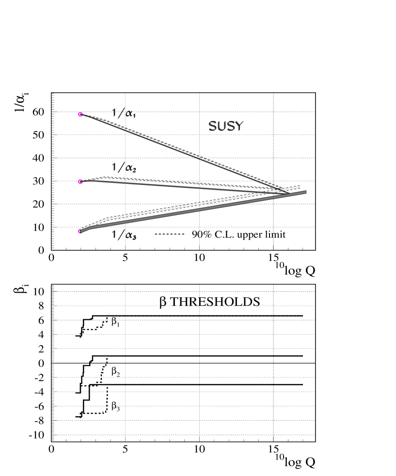
Figure 6.1: Evolution of the inverse of the three couplings in the MSSM. The line above $M_{\rm GUT}$ follows the prediction from the supersymmetric SU(5) model. The SUSY thresholds have been indicated in the lower part of the curve: they are treated as step functions in the first order $\beta$ coefficients in the renormalization group equations, which correspond to a change in slope in the evolution of the couplings in the top figure. The dashed lines correspond to the 90% C.L. upper limit for the SUSY thresholds.

The upper part of fig. 6.1 shows the evolution of the coupling constants in the MSSM for two cases: one for the minimum value of the $\chi^{2}$ function given in eq. LABEL:chi2 (solid lines) and one corresponding to the 90% C.L. upper limit of the thresholds of the light SUSY particles (dashed lines). The position of the light thresholds is shown in the bottom part as jumps in the first order $\beta$ coefficients, which are increased according to the entries in table A.1 as soon as a new threshold is passed. Also the second order coefficients are changed correspondingly (see table A.2), but their effect on the evolution is not visible in the top figure in contrast to the first order effects, which change the slope of the lines considerably in the top figure. One observes that the changes in the coupling constants occur in a rather narrow energy regime, so qualitatively this picture is very similar to fig. 4.1, in which case all sparticles were assumed to be degenerate at an effective SUSY mass scale ${M_{SUSY}}$[11]. Since the running of the couplings depends only logarithmically on the sparticle masses, the 90% C.L. upper limits are as large as several TeV, as shown by the dashed lines in fig. 6.1 and more quantitatively in table 6.1. In this table the initial choices of ${m_{0}}$ and ${\tan\beta}$ as well as the fitted parameters ${\alpha_{GUT}},\ {M_{GUT}},\ {m_{1/2}},\ \mu,\ Y_{t}(0)$ (and the corresponding top mass after running down $Y_{t}$ from ${M_{GUT}}$ to ${m_{t}}$) are shown at the top and given these parameters the corresponding masses of the SUSY particles can be calculated. Their values are given in the lower part of the table. Note we fitted here five parameters with five constraints, so the $\chi^{2}$=0, if a good solution can be found. This is indeed the case. The upper and lower limits in table 6.1 will be discussed below.

Only the value of the top Yukawa coupling is given, since for the ratio of bottom and tau mass only the ratio of the Yukawa couplings enters, not their absolute values. For the running of the gauge couplings and the mixing in the quark sector, only the small contribution from the top Yukawa coupling is taken into account, since for the range of ${\tan\beta}$ considered, all other Yukawa contributions are negligible.

As mentioned before, varying $A_{t}(0)$ between $+3{m_{0}}$ and $-3{m_{0}}$ does not influence the results very much, so its value at the unification scale was kept at 0, but its non-zero value at lower energies due to the large radiative corrections was taken into account. The fits are shown for positive values of the Higgs mixing paramter $\mu$, but similar values are obtained for negative values of $\mu$ with an equally good $\chi^{2}$ value for the fit.

The parameters ${m_{0}},~{}{m_{1/2}}$ and $\mu$ are correlated, as shown in fig. 6.2, where the value of $\mu$ is shown for all combinations of ${m_{0}}$ and ${m_{1/2}}$ between 100 and 1000 GeV. One observes that $\mu$ increases with increasing $m_{0}$  and ${m_{1/2}}$. The strong correlation between ${m_{1/2}}$ and $\mu$ originates mainly from the electroweak symmetry breaking condition, but also from the fact that the thresholds in the running of the gauge couplings all have to occur at a similar scale. For example, from fig. 6.1 it is obvious that the dashed lines for $1/\alpha_{1}$ and $1/\alpha_{2}$ will not meet with the solid line of $1/\alpha_{3}$, simply because the thresholds are too different; the thresholds in $1/\alpha_{3}$ are mainly determined by ${m_{1/2}}$, while the thresholds for the upper two lines include the winos and higgsinos too, so one obtains automatically a positive correlation between $\mu$ and ${m_{1/2}}$.

The $\chi^{2}$ value is acceptable in the whole region, except for the regions where either ${m_{0}}$ or ${m_{1/2}}$ or both become very small, as shown in fig. 6.3. The increase in this corner is completely due to the constraint from the proton lifetime (see section 6.5). This plot was made for ${\tan\beta}=2$. For larger values the region excluded by proton decay quickly increases; for ${\tan\beta}=10$ practically the whole region is excluded.

One notices from fig. 6.2 already a strong correlation between $\mu$ and ${m_{1/2}}$. This is explicitly shown in fig. 6.4. The steep walls originate from the experimental lower limits on the SUSY masses and the requirement of radiative symmetry breaking. In the minimum the $\chi^{2}$ value is zero, but one notices a long valley, where the $\chi^{2}$ is only slowly increasing. Consequently, the upper limits on the sparticle masses, which grow with increasing values of $\mu$ and ${m_{1/2}}$, become several TeV, as shown in table 6.1. The 90% C.L. upper limits were obtained by requiring an increase in $\chi^{2}$ of 1.64. so the rather The upper limits are a sensitive function of the central value of ${\alpha_{s}}$: decreasing the central value of ${\alpha_{s}}$ by two standard deviations (i.e. 0.012) can increase the thresholds of sparticles several TeV. Acceptable fits are only obtained for input ${\alpha_{s}}$ values between 0.108 and 0.132, if the error is kept at 0.006. Outside this range all requirements cannot be met simultaneously any more, so the MSSM predicts ${\alpha_{s}}$ in this range.

As discussed previously, sparticle masses in the TeV range spoil the cancellation of the quadratic divergences. This can be seen explicitly in the corrections to ${M_{Z}}$: $\Delta_{Z}$ is exactly zero if the masses of stop– and top quarks are identical, but the corrections grow quickly if the degeneracy is removed, as shown in fig. 6.5. For the SUSY masses at the minimum value of $\chi^{2}$ the corrections to ${M_{Z}}$ are small. If one requires that only solutions are allowed for which the corrections to ${M_{Z}}$ are not large compared with ${M_{Z}}$ itself, one has to limit the mass of the heaviest stop quark to about one TeV. The corresponding 90% C.L. upper limits of the individual sparticles masses are given in the right hand column of table 6.1. The correction to ${M_{Z}}$ is 6 times $M_{Z}$  in this case. The limits are obtained by scanning ${m_{0}}$ and ${m_{1/2}}$ till the $\chi^{2}$ value increases by 1.64, while optimizing the values of ${\tan\beta},~{}\mu,~{},{\alpha_{GUT}},~{}Y_{t}(0)$ and ${M_{GUT}}$. The lower limits on the SUSY parameters are shown in the left column of table 6.1. The lowest values of ${m_{0}}=45$ GeV and ${m_{1/2}}$=85 GeV are required to have simultaneously a sneutrino mass above 42 GeV and a wino mass above 45 GeV. If the proton lifetime is included, the minimum value of either ${m_{0}}$ or ${m_{1/2}}$ have to increase (see fig. 6.2). Since the squarks and gauginos are much more sensitive to ${m_{1/2}}$, one obtains the lower limits by increasing ${m_{0}}$. The minimum value for ${m_{0}}$ is about 400 GeV in this case. But in both cases the $\chi^{2}$ increase for the lower limits is due to the b-mass, which is predicted to be 4.6 GeV from the parameters determining the lower limits.

The b-quark mass is a strong function of both ${\tan\beta}$ and ${m_{t}}$, as shown in fig. 6.6; this dependence originates from the $W-t$ loop to the bottom quark. The horizontal band corresponds to the mass of the b-quark after QCD corrections: ${m_{b}}=4.25\pm 0.3$ GeV (see eq. 6.20). Since also ${M_{Z}}$ is a strong function of the same parameters, the requirement of gauge and Yukawa coupling unification together with electroweak symmetry breaking strongly constrains the SUSY particle spectrum. A typical fit with a $\chi^{2}$ equal zero is given in the central column of table 6.1, but is should be noted that the values in the other columns provide acceptable fits too at the 90% C.L..

The mass of the lightest Higgs particle, called $h$ in table 6.1, is a rather strong function of $m_{t}$, as shown in fig. 6.7 for various choices of ${\tan\beta}$, ${m_{0}}$ and ${m_{1/2}}$. All other parameters were optimized for these inputs and after the fit the values of the Higgs and top mass were calculated and plotted. One observes that the mass of the lightest Higgs particle varies between 60 and 150 GeV and the top mass between 134 and 190 GeV. Furthermore, it is evident that ${\tan\beta}$ almost uniquely determines the value of ${m_{t}}$, since even if ${m_{1/2}}$ and ${m_{0}}$ are varied between 100 and 1000 GeV, one finds the practically the same ${m_{t}}$ for a given ${\tan\beta}$ and the value of ${m_{t}}$ varies between 134 and 190 GeV, if ${\tan\beta}$ is varied between 1.2 and 5. This range is in excellent agreement with the estimates given in eq. 6.19, if one takes into account that $M_{t}^{pole}\approx 1.06{m_{t}}$ (see eq. 6.18).

Note the strong correlation between ${\tan\beta}$ and ${m_{t}}$ in fig. 6.7: for a given value of ${\tan\beta}$ ${m_{t}}$ is constrained to a vary narrow range almost independent of ${m_{1/2}}$ and ${m_{0}}$. Furthermore one observes a rather strong positive correlation between $m_{h}iggs$ and all other parameters (${\tan\beta},~{}{m_{0}},~{}$ and ${m_{1/2}}$) originating from the loop corrections to the potential.

In summary, the following parameter ranges are allowed (if the limit on proton lifetime is obeyed and extreme finetuning is to be avoided, i.e. $\tilde{m}_{t2}<1$ TeV):

$$400~{}< ~{}m_{0}~{} <~{}1000~{}\mbox{GeV}$$

$$80~{}< ~{}m_{1/2}~{} <~{}475~{}\mbox{GeV}$$

$$330~{}< ~{}\mu~{} <~{}1100~{}\mbox{GeV}$$

$$1~{}< ~{}\tan\beta~{} <~{}10$$

$$134~{}< ~{}m_{t}~{} <~{}190~{}\mbox{GeV~{}(from fig. \ref{f67}.)}$$

$$0.108~{}< ~{}\alpha_{s}~{} <~{}0.132$$

The corresponding constraints on the SUSY masses are (see table 6.1 for details):

$$25~{}< \chi^{0}_{1}(\tilde{\gamma}) <~{}202~{}\mbox{GeV}$$

$$48~{}< \chi^{0}_{2}(\tilde{Z}),\chi^{\pm}_{1}(\tilde{W}) <~{}386~{}\mbox{GeV}$$

$$217~{}< \tilde{g} <~{}1104~{}\mbox{GeV}$$

$$440~{}< \tilde{q} <~{}1070~{}\mbox{GeV}$$

$$240~{}< \tilde{t}_{1} <~{}725~{}\mbox{GeV}$$

$$414~{}< \tilde{t}_{2} <~{}1000~{}\mbox{GeV}$$

$$406~{}< \tilde{e}_{L} <~{}521~{}\mbox{GeV}$$

$$401~{}< \tilde{e}_{R} <~{}440~{}\mbox{GeV}$$

$$400~{}< \tilde{\nu}_{L} <~{}516~{}\mbox{GeV}$$

$$291~{}< \chi^{0}_{3}(\tilde{H}_{1}) <~{}799~{}\mbox{GeV}$$

$$313~{}< \chi^{0}_{4}(\tilde{H}_{2}) <~{}812~{}\mbox{GeV}$$

$$315~{}< \chi^{\pm}_{2}(\tilde{H}^{\pm}) <~{}831~{}\mbox{GeV}$$

$$527~{}< H^{\pm} <~{}1034~{}\mbox{GeV}$$

$$523~{}< {H} <~{}1033~{}\mbox{GeV}$$

$$521~{}< {A} <~{}1031~{}\mbox{GeV}$$

$$60~{}< {h} <~{}150~{}\mbox{GeV ~{}(from fig. \ref{f67}.)}$$

The lower limits will all increase as soon as the LEP limits on sneutrinos, winos and the lightest Higgs increase.

The lightest Higgs particle is certainly within reach of experiments at present or future accelerators[112, 113]. Its observation in the predicted mass range of 60 to 150 GeV would be a strong case in support of this minimal version of a supersymmetric grand unified theory.

Figure 6.2: The fitted MSSM parameter $\mu$ as function of ${m_{0}}$ and ${m_{1/2}}$ for ${\tan\beta}=2$.

Figure 6.3: The $\chi^{2}$ of the fit as function of ${m_{0}}$ and ${m_{1/2}}$ for ${\tan\beta}=2$. The sharp increase in $\chi^{2}$ in the corner is caused by the lower limit on the proton lifetime.

Figure 6.4: The correlation between ${m_{1/2}}$ and $\mu$ for ${m_{0}}$=500 GeV.

Figure 6.5: The one-loop correction factor to ${M_{Z}}$ as function of ${m_{0}}$ and ${m_{1/2}}$.

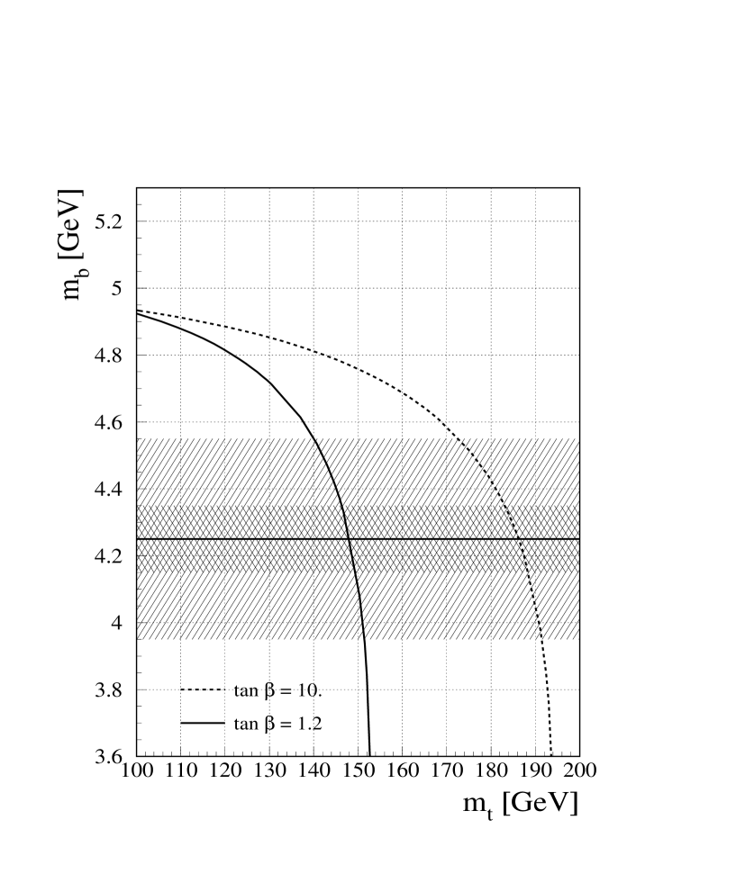
Figure 6.6: The correlation between ${m_{b}}$ and ${m_{t}}$ for ${m_{0}}$=400 GeV and two values of ${\tan\beta}$. The hatched area indicates the experimental value for $m_{b}$.

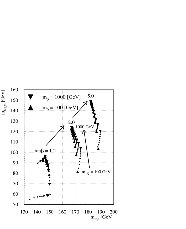
Figure 6.7: The mass of the lightest Higgs particle as function of the top quark mass for values of ${\tan\beta}$ between 1.2 and 5 and values of ${m_{0}}$ and ${m_{1/2}}$ between 100 and 1000 GeV. The parameters of $\mu,~{}{M_{GUT}},~{}{\alpha_{GUT}}$ and $Y_{t}(0)$ are optimized for each choice of these parameters; the corresponding values of the top and lightest Higgs mass are shown as symbols. For small values of ${m_{1/2}}$ the Higgs mass increases with ${m_{0}}$, as shown for a “string” of points, each representing a step of 100 GeV in ${m_{0}}$ for a given value of ${m_{1/2}}$, which is increasing in steps of 100 GeV, starting with the low values for the lowest strings. At high values of ${m_{1/2}}$ the value of ${m_{0}}$ becomes irrelevant and the “string” shrinks to a point. Note the strong positive correlation between $m_{higgs}$ and all other parameters: the highest value of the Higgs mass corresponds to the maximum values of the input parameters, i.e. ${\tan\beta}=5$, ${m_{0}}={m_{1/2}}=1000$ GeV; this value does not correspond to the minimum $\chi^{2}$. More likely values correspond to $m_{higgs}\approx 92$ GeV for ${m_{1/2}}=100$, ${m_{0}}=400$ and ${\tan\beta}=2$.

Symbol	Lower limits		Typical fit	90% C.L. Upper limits
Constraints	GEY	GEY+P	GEY+(PF)	GEY+ (P)	GEY+(P)+F
Fitted SUSY parameters
$m_{0}$	45	400	400	400	400
$m_{1/2}$	85	80	111	1600	475
$\mu$	170	330	633	1842	1101
$\tan\beta$	20.	3.0	2.3	8.5	2.9
$Y_{t}(0)$	0.0047	0.0035	0.0140	0.0023	0.0084
$m_{t}$	184	172	177	168	178
$1/\alpha_{GUT}$	24.0	24.3	24.5	25.9	25.2
$M_{GUT}$	$2.0\;10^{16}$	$2.0\;10^{16}$	${\bf 2.0\;10^{16}}$	$0.8\;10^{16}$	$1.3\;10^{16}$
SUSY masses in [GeV]
$\chi^{0}_{1}(\tilde{\gamma})$	28	25	40	720	202
$\chi^{0}_{2}(\tilde{Z})$	52	52	78	1346	386
$\chi^{\pm}_{1}(\tilde{W})$	49	48	76	1347	386
$\tilde{g}$	235	217	293	3377	1105
$\tilde{e}_{L}$	90	406	410	1160	521
$\tilde{e}_{R}$	56	401	402	729	440
$\tilde{\nu}_{L}$	42	400	404	1157	516
$\tilde{q}_{L}$	221	443	477	3030	1071
$\tilde{q}_{R}$	213	440	471	2872	1030
$\tilde{b}_{L}$	200	352	370	2610	903
$\tilde{b}_{R}$	215	440	471	2862	1027
$\tilde{t}_{1}$	181	240	213	2333	725
$\tilde{t}_{2}$	311	414	450	2817	1008
$\chi^{0}_{3}(\tilde{H}_{1})$	157	292	404	1771	799
$\chi^{0}_{4}(\tilde{H}_{2})$	181	313	423	1780	812
$\chi^{\pm}_{2}(\tilde{H}^{\pm})$	186	315	429	1816	831
$h$	105	96	97	146	127
$H$	145	523	629	2218	1033
$A$	145	521	627	2217	1031
$H^{\pm}$	165	527	631	2219	1034

Table 6.1: Values of SUSY masses and parameters for various constraints: G=gauge coupling unification; E=electroweak symmetry breaking; Y=Yukawa coupling unification; P=Proton lifetime constraint; F=finetuning constraint. Constraints in brackets indicate that they are fulfilled but not required. The value of the lightest Higgs $h$ can be lower than indicated (see text).

Chapter 7 Summary.

Many of the questions posed by cosmology suggest phase transitions during the evolution of the universe from the Planck temperature of $10^{32}$ K to the 2.7 K observed today. Among them the baryon asymmetry in our universe and inflation, which is the only viable solution to explain the horizon problem, the flatness problem, the magnetic monopole problem, and the smoothness problem (see chapter 5).

In Grand Unified Theories (GUT) phase transitions are expected: one at the unification scale of $10^{16}$ GeV, i.e. at a temperature of about $10^{28}$ K and one at the electroweak scale, i.e. at a temperature of about $10^{14}$ K. Furthermore, scalar fields, which are a prerequisite for inflation, are included in GUT’s. In the minimal model at least 29 scalar fields are required. Unfortunately, none have been discovered so far, so little is known about the scalar sector, although the verification of the relation between the couplings and the masses of the electroweak gauge bosons indeed are indirect evidence that their mass is generated by the interaction with a scalar field. Experimental observation of these scalar fields would provide a great boost for cosmology and particle physics. First estimates of the required mass spectra of the scalar fields can be obtained by comparing the experimental consequences of Grand Unified Theories (GUT) with low energy phenomenology.

One of the interesting “discoveries” of LEP was the fact that within the Standard Model (SM) unification of the gauge couplings could be excluded (see fig. 4.1). In contrast, the minimal supersymmetric extension of the SM (MSSM) provided perfect unification. This observation boosted the interest in Supersymmetry enormously, especially since the MSSM was not “designed” to provide unification, but it was invented many years ago and turned out to have very interesting properties:

• Supersymmetry automatically provides gravitational interactions, thus paving the road for a “Theory Of Everything”.

• The symmetry between bosons and fermions alleviates the divergences in the radiative corrections, in which case these corrections can be made responsible for the electroweak symmetry breaking at a much lower scale than the GUT scale.

• The lightest supersymmetric partner (LSP) is a natural candidate for non-relativistic dark matter in our universe.

Other non-supersymmetric models can yield unification too,but they do not exhibit the elegant symmetry properties of supersymmetry, they offer no explanation for dark matter and no explanation for the electroweak symmetry breaking. Furthermore the quadratic divergences in the radiative corrections do not cancel.

The Minimal Supersymmetric Standard Model (MSSM) model has many predictions, which can be compared with experiment, even in the energy range where the predicted SUSY particles are out of reach. Among these predictions:

• $M_{Z}$.

• $m_{b}$.

• Proton decay.

• Dark matter.

It is surprising, that in addition to the unification of the coupling c onstants the minimal supersymmetric model can fulfil all experimental constraints from these predictions. As far as we know, supersymmetric models are the only ones, which are consistent with all these observations simultaneously.

Figure 7.1: Possible evolution of the radius of the universe and the coupling constants. Before $t=10^{-38}$ s spontaneous symmetry breaking occurs, which breaks the symmetry of the GUT into the well known symmetries at low energies. In the mean time the universe inflates to a size far above the distance light could have traveled as indicated by the dashed line. From [114].

Within the MSSM the evolution of the universe can be traced back to about $10^{-38}$ seconds after the ‘bang’, as sketched in fig. 7.1. If we believe in the inflationary scenario even the actual creation of the universe is describable by physical laws. In this view the universe would originate as a quantum fluctuation, starting from absolute “nothing”, i.e. a state devoid of space, time and matter with a total energy equal to zero. Indeed, estimates of the total positive non-gravitational energy and negative potential energy are about equal in our universe, i.e. according to this view the universe is the ultimate “free lunch”. All this mass was generated from the potential energy of the vacuum, which also caused the inflationary phase.

Of course, a quantum description of space-time can be discussed only in the context of quantum gravity, so these ideas must be considered speculative until a renormalizable theory of quantum gravity is formulated and proven by experiment. Nevertheless, it is fascinating to contemplate that physical laws may determine not only the evolution of our universe, but they may remove also the need for assumptions about the initial conditions.

From the experimental constraints at low energies the mass spectra for the SUSY particles can be predicted (see table 6.1 in the previous chapter). The lightest Higgs particle is certainly within reach of experiments at present or future accelerators. Its observation in the predicted mass range of 60 to 150 GeV would be a strong case in support of this minimal version of the supersymmetric grand unified theory. Discovering also the heavier SUSY particles implies that the known strong, electromagnetic and weak forces were all unified into a single “primeval” force during the birth of our universe. Future experiments will tell!

Acknowledgments.

I want to thank sincerely Ugo Amaldi, Hermann Fürstenau, Ralf Ehret and Dmitri Kazakov for their close collaboration in this exciting field. Without their enthusiasm, work and sharing of ideas many of our common results presented in this review would not have been available. Furthermore, I thank John Ellis, Gian Giudice, Howie Haber, Gordy Kane, Stavros Katsanevas, Sergey Kovalenko, Hans Kühn, Jorge Lopez, Dimitri Nanopoulos, Pran Nath, Dick Roberts, Leszek Roszkowski, Mikhail Shaposhnikov, William Trischuk, and Fabio Zwirner for helpful discussions and/or commenting parts of the manuscript.

Last, but not least, I want to thank Prof. Faessler for inviting me to a seminar in Tübingen and his encouragement to write down the results presented there in this review.

Appendix A

A.1 Introduction

In this appendix all the Renormalization Group Equations (RGE) for the evolution of the masses and the couplings are given. SUSY particles influence the evolution only through their appearance in the loops, so they enter only in higher order. Therefore it is sufficient to consider the loop corrections to the masses only in first order, in which case a simple analytical solution can be found, even if the one-loop correction to the Higgs potential from the top Yukawa coupling is taken into account. There is one exception: the corrections to the bottom and tau mass are compared directly with data, which implies that the second order solutions have to be taken for the RGE predicting the ratio of the bottom and tau mass. Since this ratio involves the top Yukawa coupling $Y_{t}$, the RGE for $Y_{t}$ has to be considered in second order too. These second order corrections are important for the bottom mass, since the strong coupling constant becomes large at the small scale of the bottom mass, i.e. $\alpha_{s}(m_{b})\approx 0.2$.

So in total one has to solve a system of 18 coupled differential equations (5 second order, 13 first order):

• 3 second order equations for the running of the gauge coupling constants $\alpha_{i},~{}i=1,3$;

• 2 second order equations for the running of the top Yukawa coupling $Y_{t}$ and the ratio of bottom and tau Yukawa coupling $R_{b\tau}$;

• 1 first order equation for the masses of the left-handed doublet of an u-type and d-type squark pair $Q$;

• 1 first order equation for the masses of the right-handed up-type squarks $U$;

• 1 first order equation for the masses of the right-handed down-type squarks $D$;

• 1 first order equation for the masses of the left-handed doublet of sleptons $L$;

• 1 first order equation for the masses of the right-handed singlet of a charged lepton $E$;

• 4 first order equations for the 4 mass parameters of the Higgs potential ($m_{1},m_{2},m_{3},$ and $\mu$);

• 3 first order equations for the (Majorana) masses of the gauginos ($M_{1},M_{2}$ and $M_{3}$).

• 1 first order equation for the trilinear coupling between left- and right handed squarks and the Higgs field $A_{t}$, where the subscript indicates that one only considers this coupling for the third generation.

Note that the absolute values of the bottom and tau Yukawa couplings need not to be known, if one neglects their small contribution to the running of the gauge couplings. If one wants to include these, one has to integrate the RGE for $Y_{b}$ and $Y_{\tau}$ separately (they are given below too) instead of the RGE for their ratio only. Integrating the ratio has the advantage, that the boundary condition at ${M_{GUT}}$ is known to be one, if one assumes Yukawa coupling unification.

The particle masses are related directly to the Yukawa couplings:

$$Y_{t}(m_{t}) = \frac{h_{t}^{2}}{(4\pi)^{2}};\ \ \ \ \ m_{t}=h_{t}(m_{t})\ v\ \sin\beta$$ (A.1)

$$Y_{b}(m_{b}) = \frac{h_{b}^{2}}{(4\pi)^{2}};\ \ \ \ \ \ m_{b}=h_{b}(m_{b})\ v\ \cos\beta$$ (A.2)

$$Y_{\tau}(m_{\tau}) = \frac{h_{\tau}^{2}}{(4\pi)^{2}};\ \ \ \ \ \ m_{\tau}=h_{\tau}(m_{\tau})\ v\ \cos\beta.$$ (A.3)

It follows that

$$\frac{Y_{t}}{Y_{b}}=\frac{m_{t}^{2}}{m_{b}^{2}}\frac{1}{\tan^{2}\beta}.$$ (A.4)

For ${\tan\beta}<10$, as required by proton decay limits, one observes that $Y_{b}$ is at least an order of magnitude smaller than $Y_{t}$ for the values of $m_{t}$ considered. Hence its contribution is indeed negligible in the running of the gauge couplings, so below we will only consider the contribution of $Y_{b}$ in the ratio of $Y_{b}/Y_{\tau}$, which is independent of the absolute value of $Y_{b}(0)$.

Below we collect all the RGE’s in a coherent notation and consider the coefficients for the various threshold regions, i.e. virtual particles with mass $m_{i}$ are considered to contribute to the running of the gauge coupling constants effectively only for $Q$ values above $m_{i}$. Thus the thresholds are treated as simple step functions in the coefficients of the RGE.

Furthermore, all first order solutions are given in an analytical form, including the corrections from the top Yukawa coupling[115]. Note that a more demanding analysis requires a numerical solution of the first five second order equations, in which the coefficients are changed according to the thresholds found as analytical solutions of the first order equations for the evolution of the masses. The results given in chapter 6 all use the numerical solution of these second order equation.

Using the supergravity inspired breaking terms, which assume a common mass $m_{1/2}$ for the gauginos and another common mass $m_{0}$ for the scalars, leads to the following breaking term in the Lagrangian:

$${\cal L}_{Breaking} = -m_{0}^{2}\sum_{i}|\varphi_{i}|^{2}-m_{1/2}\sum_{\alpha}\lambda_{\alpha}\lambda_{\alpha}$$ (A.5)

$$- Am_{0}\left[h^{u}_{ab}Q_{a}U^{c}_{b}H_{2}+h^{d}_{ab}Q_{a}D^{c}_{b}H_{1}+h^{e}_{ab}L_{a}E^{c}_{b}H_{1}\right]-Bm_{0}\left[\mu H_{1}H_{2}\right].$$ (A.6)

Here

$h^{u,d,e}_{ab}$	are the Yukawa couplings,  $a,b=1,2,3$ run over the generations
$Q_{a}$	are the SU(2) doublet quark fields
$U_{a}^{c}$	are the SU(2) singlet charge-conjugated up-quark fields
$D_{b}^{c}$	are the SU(2) singlet charge-conjugated down-quark fields
$L_{a}$	are the SU(2) doublet lepton fields
$E_{a}^{c}$	are the SU(2) singlet charge-conjugated lepton fields
$H_{1,2}$	are the SU(2) doublet Higgs fields
$\varphi_{i}$	are all scalar fields
$\lambda_{\alpha}$	are the gaugino fields

The last two terms in ${\cal{L}}_{Breaking}$ originate from the cubic and quadratic terms in the superpotential with A, B and $\mu$ as free parameters. In total we now have three couplings $\alpha_{i}$ and five mass parameters:

$$m_{0},~{}m_{1/2},~{}\mu(t),~{}A(t),~{}B(t).$$

with the following boundary conditions at ${M_{GUT}}$ $(t=0)$:

$${\rm scalars:} \tilde{m}^{2}_{Q}=\tilde{m}^{2}_{U}=\tilde{m}^{2}_{D}=\tilde{m}^{2}_{L}=\tilde{m}^{2}_{E}=m_{0}^{2};$$ (A.7)

$${\rm gauginos:} M_{i}=m_{1/2},\ \ \ i=1,2,3;$$ (A.8)

$${\rm couplings:} \tilde{\alpha}_{i}(0)=\tilde{\alpha}_{GUT},\ \ \ i=1,2,3.$$ (A.9)

Here $M_{1}$, $M_{2}$, and $M_{3}$ are the gauginos masses of the $U(1)$, $SU(2)$ and $SU(3)$ groups.In $N=1$ supergravity one expects at the Planck scale $B=A-1$.

With these parameters and the initial conditions at the GUT scale the masses of all SUSY particles can be calculated via the renormalization group equations.

A.2 Gauge Couplings

The following definitions are used:

$$\tilde{\alpha}_{i} = \frac{\alpha_{i}}{4\pi}$$ (A.10)

$$t = \ln(\frac{{M_{GUT}^{2}}}{Q^{2}})$$ (A.11)

$$\beta_{i} = b_{i}~{}\tilde{\alpha}_{GUT}$$ (A.12)

$$f_{i}(t) = \frac{1}{\beta_{i}}\left(1-\frac{1}{(1+\beta_{i}t)^{2}}\right)$$ (A.13)

$$h_{i}(t) = \frac{t}{(1+\beta_{i}t)},$$ (A.14)

where $\alpha_{i}$ (i=1,3) denote the three gauge coupling constants of $U(1)$, $SU(2)andSU(3)$, respectively, $\alpha_{GUT}$ is the common gauge coupling at the GUT scale ${M_{GUT}}$ and $b_{i}$ are the coefficients of the RGE, as defined below.

The second order RGE’s for the gauge couplings including the effect of the Yukawa couplings are[97, 71, 116]:

$$\frac{d\tilde{\alpha}_{i}}{dt} = -b_{i}\tilde{\alpha}_{i}^{2}-\tilde{\alpha}_{i}^{2}\left(\sum_{j}b_{ij}\tilde{\alpha}_{j}-a_{i}Y_{t}\right),$$ (A.15)

where $a_{1}=\frac{26}{5},a_{2}=6,a_{3}=4$ for SUSY and $a_{1}=\frac{17}{10},a_{2}=\frac{3}{2},a_{3}=2$ for the SM.

The first order coefficients for the SM are[117]:

$$b_{i}=\left(\begin{array}[]{r}b_{1}\\ b_{2}\\ b_{3}\end{array}\right)=\left(\begin{array}[]{r}0\\ -22/3\\ -11\end{array}\right)+N_{Fam}\left(\begin{array}[]{r}4/3\\ 4/3\\ 4/3\end{array}\right)+N_{Higgs}\left(\begin{array}[]{r}1/10\\ 1/6\\ 0\end{array}\right),$$ (A.16)

while for the supersymmetric extension of the SM (to be called MSSM in the following)[117]:

$$b_{i}=\left(\begin{array}[]{r}b_{1}\\ b_{2}\\ b_{3}\end{array}\right)=\left(\begin{array}[]{r}0\\ -6\\ -9\end{array}\right)+N_{Fam}\left(\begin{array}[]{r}2\\ 2\\ 2\end{array}\right)+N_{Higgs}\left(\begin{array}[]{r}3/10\\ 1/2\\ 0\end{array}\right),$$ (A.17)

Here $N_{Fam}$ is the number of families of matter supermultiplets and $N_{Higgs}$ is the number of Higgs doublets. We use $N_{Fam}=3$ and $N_{Higgs}=1$ or 2, which corresponds to the minimal SM or minimal SUSY model, respectively.

The second order coefficients are:

$$b_{ij}=\left(\begin{array}[]{rrr}\rule{0.0pt}{14.22636pt}0&0&0\\ \rule{0.0pt}{14.22636pt}0&-\frac{136}{3}&0\\ \rule{0.0pt}{14.22636pt}0&0&-102\end{array}\right)+N_{Fam}\left(\begin{array}[]{rrr}\rule{0.0pt}{14.22636pt}\frac{19}{15}&\frac{3}{5}&\frac{44}{15}\\ \rule{0.0pt}{14.22636pt}\frac{1}{5}&\frac{49}{3}&4\\ \rule{0.0pt}{14.22636pt}\frac{11}{30}&\frac{3}{2}&\frac{76}{3}\end{array}\right)+N_{Higgs}\left(\begin{array}[]{rrr}\rule{0.0pt}{14.22636pt}\frac{9}{50}&\frac{9}{10}&0\\ \rule{0.0pt}{14.22636pt}\frac{3}{10}&\frac{13}{6}&0\\ \rule{0.0pt}{14.22636pt}0&0&0\end{array}\right).$$ (A.18)

For the SUSY model they become:

$$b_{ij}=\left(\begin{array}[]{rrr}\rule{0.0pt}{14.22636pt}0&0&0\\ \rule{0.0pt}{14.22636pt}0&-24&0\\ \rule{0.0pt}{14.22636pt}0&0&-54\end{array}\right)+N_{Fam}\left(\begin{array}[]{rrr}\rule{0.0pt}{14.22636pt}\frac{38}{15}&\frac{6}{5}&\frac{88}{15}\\ \rule{0.0pt}{14.22636pt}\frac{2}{5}&14&8\\ \rule{0.0pt}{14.22636pt}\frac{11}{15}&3&\frac{68}{3}\end{array}\right)+N_{Higgs}\left(\begin{array}[]{rrr}\rule{0.0pt}{14.22636pt}\frac{9}{50}&\frac{9}{10}&0\\ \rule{0.0pt}{14.22636pt}\frac{3}{10}&\frac{7}{2}&0\\ \rule{0.0pt}{14.22636pt}0&0&0\end{array}\right).$$ (A.19)

The contributions for the individual thresholds to $b_{i}$ and $b_{ij}$ are listed in tables A.1 (from ref. [66]) and A.2, respectively.

The running of each $\alpha_{i}$ depends on the values of the two other coupling constants, if the second order effects are taken into account. However, these effects are small, because the $b_{ij}$’s are multiplied by ${\alpha_{j}}/{4\pi}\leq 0.01$. Higher orders are presumably even smaller.

If the small Yukawa couplings are neglected, the RGE’s A.15 can be solved by integration to obtain $\alpha_{i}^{\prime}(\mu^{\prime})$ at a scale $\mu^{\prime}$ for a given $\alpha_{i}(\mu)$:

$$\alpha_{i}^{\prime}(\mu^{\prime})=\left[\beta_{0}\cdot\ln\frac{\mu^{\prime 2}}{\mu^{2}}+\frac{1}{\alpha_{i}(\mu)}+\frac{\beta_{1}}{\beta_{0}}\ln\left(\frac{1/\alpha_{i}^{\prime}(\mu^{\prime})+\beta_{1}/\beta_{0}}{1/\alpha_{i}(\mu)+\beta_{1}/\beta_{0}}\right)\right]^{-1}$$ (A.20)

with

$$\beta_{0} = \frac{-1}{2\pi}\left(b_{i}+\frac{b_{ij}}{4\pi}\alpha_{j}(\mu)+\frac{b_{ik}}{4\pi}\alpha_{k}(\mu)\right)$$ (A.21)

$$\beta_{1} = \frac{-2\cdot b_{ii}}{(4\pi)^{2}}.$$ (A.22)

This exact solution to the second order renormalization group equation can be used to calculate the coupling constants at an arbitrary energy, if they have been measured at a given energy, i.e. one calculates $\alpha_{i}(\mu^{\prime})$ from a given $\alpha_{i}(\mu)$. This transcendental equation is most easily solved numerically by iteration. If the Yukawa couplings are included, their running has to be considered too and one can solve the coupled equations of gauge couplings and Yukawa couplings only numerically.

A.3 Yukawa Couplings

In order to calculate the evolution of the Yukawa coupling for the b quark in the region between $m_{b}$ and ${M_{GUT}}$, one has to consider four different threshold regions:

• Region I between the typical sparticle masses ${M_{SUSY}}$ and the GUT scale.

• Region II between ${M_{SUSY}}$ and the top mass $m_{t}$.

• Region III between $m_{t}$ and $M_{Z}$.

• Region IV between $M_{Z}$ and $m_{b}$.

A.3.1 RGE for Yukawa Couplings in Region I

The second order RGE for the three Yukawa couplings of the third generation in the regions between ${M_{SUSY}}$ and ${M_{GUT}}$ are[118]:

$$\frac{dY_{t}}{dt} = Y_{t}\left(\frac{16}{3}\tilde{\alpha}_{3}+3\tilde{\alpha}_{2}+\frac{13}{15}\tilde{\alpha}_{1}-6Y_{t}\right.$$ (A.23)

$$-(\frac{16}{3}b_{3}+\frac{128}{9})\tilde{\alpha}_{3}^{2}-(3b_{2}+\frac{9}{2})\tilde{\alpha}_{2}^{2}-(\frac{13}{15}b_{1}+\frac{169}{450})\tilde{\alpha}_{1}^{2}-8\tilde{\alpha}_{3}\tilde{\alpha}_{2}-\frac{136}{45}\tilde{\alpha}_{3}\tilde{\alpha}_{1}-\tilde{\alpha}_{2}\tilde{\alpha}_{1}$$

$$\left.-16\tilde{\alpha}_{3}Y_{t}-6\tilde{\alpha}_{2}Y_{t}-\frac{6}{5}\tilde{\alpha}_{1}Y_{t}+22Y_{t}^{2}\right)$$

$$\frac{dY_{b}}{dt} = Y_{b}\left(\frac{16}{3}\tilde{\alpha}_{3}+3\tilde{\alpha}_{2}+\frac{7}{15}\tilde{\alpha}_{1}-Y_{t}\right.$$ (A.24)

$$-(\frac{16}{3}b_{3}+\frac{128}{9})\tilde{\alpha}_{3}^{2}-(3b_{2}+\frac{9}{2})\tilde{\alpha}_{2}^{2}-(\frac{7}{15}b_{1}+\frac{49}{450})\tilde{\alpha}_{1}^{2}-8\tilde{\alpha}_{3}\tilde{\alpha}_{2}-\frac{8}{9}\tilde{\alpha}_{3}\tilde{\alpha}_{1}-\tilde{\alpha}_{2}\tilde{\alpha}_{1}$$

$$\left.-\frac{4}{5}\tilde{\alpha}_{1}Y_{t}+5Y_{t}^{2}\right)$$

$$\frac{dY_{\tau}}{dt} = Y_{\tau}\left(+3\tilde{\alpha}_{2}+\frac{9}{5}\tilde{\alpha}_{1}\right.$$ (A.25)

$$\left.-(3b_{2}+\frac{9}{2})\tilde{\alpha}_{2}^{2}-(\frac{9}{5}b_{1}+\frac{81}{50})\tilde{\alpha}_{1}^{2}-\frac{9}{5}\tilde{\alpha}_{2}\tilde{\alpha}_{1}\right)$$

If one assumes Yukawa coupling unification for particles belonging to the same multiplet, i.e. $Y_{b}=Y_{\tau}$ at the GUT scale, one can calculate easily the RGE for the ratio $R_{b\tau}(t)=m_{b}/m_{\tau}=\sqrt{Y_{b}(t)/Y_{\tau}(t)}$:

$$\frac{dR_{b\tau}}{dt} = R_{b\tau}\left(\frac{8}{3}\tilde{\alpha}_{3}-\frac{2}{3}\tilde{\alpha}_{1}-\frac{1}{2}Y_{t}\right.$$ (A.26)

$$-(\frac{8}{3}b_{3}+\frac{64}{9})\tilde{\alpha}_{3}^{2}+(\frac{2}{3}b_{1}+\frac{34}{45})\tilde{\alpha}_{1}^{2}-4\tilde{\alpha}_{3}\tilde{\alpha}_{2}-\frac{4}{9}\tilde{\alpha}_{3}\tilde{\alpha}_{1}+\frac{2}{5}\tilde{\alpha}_{2}\tilde{\alpha}_{1}$$

$$\left.-\frac{2}{5}\tilde{\alpha}_{1}Y_{t}+\frac{5}{2}Y_{t}^{2}\right)$$

A.3.2 RGE for Yukawa Couplings in Region II

For the region between $M_{SUSY}$ and $m_{t}$ one finds[119]:

$$\frac{dY_{t}}{dt} = Y_{t}\left(8\tilde{\alpha}_{3}+\frac{9}{4}\tilde{\alpha}_{2}+\frac{17}{20}\tilde{\alpha}_{1}-\frac{9}{2}Y_{t}\right.$$ (A.27)

$$+108\tilde{\alpha}_{3}^{2}+\frac{23}{4}\tilde{\alpha}_{2}^{2}-\frac{1187}{600}\tilde{\alpha}_{1}^{2}-9\tilde{\alpha}_{3}\tilde{\alpha}_{2}-\frac{19}{15}\tilde{\alpha}_{3}\tilde{\alpha}_{1}+\frac{9}{20}\tilde{\alpha}_{2}\tilde{\alpha}_{1}$$

$$\left.-36\tilde{\alpha}_{3}Y_{t}-\frac{225}{16}\tilde{\alpha}_{2}Y_{t}-\frac{393}{80}\tilde{\alpha}_{1}Y_{t}+12Y_{t}^{2}\right)$$

$$\frac{dY_{b}}{dt} = Y_{b}\left(8\tilde{\alpha}_{3}+\frac{9}{4}\tilde{\alpha}_{2}+\frac{1}{4}\tilde{\alpha}_{1}-\frac{3}{2}Y_{t}\right.$$ (A.28)

$$+108\tilde{\alpha}_{3}^{2}+\frac{23}{4}\tilde{\alpha}_{2}^{2}+\frac{127}{600}\tilde{\alpha}_{1}^{2}-9\tilde{\alpha}_{3}\tilde{\alpha}_{2}-\frac{31}{15}\tilde{\alpha}_{3}\tilde{\alpha}_{1}+\frac{27}{20}\tilde{\alpha}_{2}\tilde{\alpha}_{1}$$

$$\left.-4\tilde{\alpha}_{3}Y_{t}-\frac{99}{16}\tilde{\alpha}_{2}Y_{t}-\frac{91}{80}\tilde{\alpha}_{1}Y_{t}+\frac{1}{4}Y_{t}^{2}\right)$$

$$\frac{dY_{\tau}}{dt} = Y_{\tau}\left(\frac{9}{4}\tilde{\alpha}_{2}+\frac{9}{4}\tilde{\alpha}_{1}-3Y_{t}\right.$$ (A.29)

$$+\frac{23}{4}\tilde{\alpha}_{2}^{2}-\frac{1371}{200}\tilde{\alpha}_{1}^{2}-\frac{27}{20}\tilde{\alpha}_{2}\tilde{\alpha}_{1}$$

$$\left.-20\tilde{\alpha}_{3}Y_{t}-\frac{45}{8}\tilde{\alpha}_{2}Y_{t}-\frac{17}{8}\tilde{\alpha}_{1}Y_{t}+\frac{27}{4}Y_{t}^{2}\right)$$

$$\frac{dR_{b\tau}}{dt} = R_{b\tau}\left(4\tilde{\alpha}_{3}-\tilde{\alpha}_{1}+\frac{3}{4}Y_{t}\right.$$ (A.30)

$$+54\tilde{\alpha}_{3}^{2}+\frac{53}{15}\tilde{\alpha}_{1}^{2}-\frac{9}{2}\tilde{\alpha}_{3}\tilde{\alpha}_{2}-\frac{31}{30}\tilde{\alpha}_{3}\tilde{\alpha}_{1}+\frac{27}{20}\tilde{\alpha}_{2}\tilde{\alpha}_{1}$$

$$\left.+8\tilde{\alpha}_{3}Y_{t}-\frac{9}{32}\tilde{\alpha}_{2}Y_{t}+\frac{79}{160}\tilde{\alpha}_{1}Y_{t}-\frac{13}{4}Y_{t}^{2}\right)$$

A.3.3 RGE for Yukawa Couplings in Region III

For the region between ${m_{t}}$ and ${M_{Z}}$ one finds:

$$\frac{dY_{b}}{dt} = Y_{b}\left(8\tilde{\alpha}_{3}+\frac{9}{4}\tilde{\alpha}_{2}+\frac{1}{4}\tilde{\alpha}_{1}\right.$$ (A.31)

$$\left.+108\tilde{\alpha}_{3}^{2}+\frac{23}{4}\tilde{\alpha}_{2}^{2}+\frac{127}{600}\tilde{\alpha}_{1}^{2}-9\tilde{\alpha}_{3}\tilde{\alpha}_{2}-\frac{31}{15}\tilde{\alpha}_{3}\tilde{\alpha}_{1}+\frac{27}{20}\tilde{\alpha}_{2}\tilde{\alpha}_{1}\right)$$

$$\frac{dY_{\tau}}{dt} = Y_{\tau}\left(\frac{9}{4}\tilde{\alpha}_{2}+\frac{9}{4}\tilde{\alpha}_{1}\right.$$ (A.32)

$$\left.+\frac{23}{4}\tilde{\alpha}_{2}^{2}-\frac{1371}{200}\tilde{\alpha}_{1}^{2}-\frac{27}{20}\tilde{\alpha}_{2}\tilde{\alpha}_{1}\right)$$

$$\frac{dR_{b\tau}}{dt} = R_{b\tau}\left(4\tilde{\alpha}_{3}-\tilde{\alpha}_{1}\right.$$ (A.33)

$$\left.+54\tilde{\alpha}_{3}^{2}+\frac{53}{15}\tilde{\alpha}_{1}^{2}-\frac{9}{2}\tilde{\alpha}_{3}\tilde{\alpha}_{2}-\frac{31}{30}\tilde{\alpha}_{3}\tilde{\alpha}_{1}+\frac{27}{20}\tilde{\alpha}_{2}\tilde{\alpha}_{1}\right)$$

A.3.4 RGE for Yukawa Couplings in Region IV

$$\frac{dR_{b\tau}}{dt} = R_{b\tau}\left(4\tilde{\alpha}_{3}-\tilde{\alpha}_{1}+54\tilde{\alpha}_{3}^{2}+\frac{53}{15}\tilde{\alpha}_{1}^{2}-\frac{31}{30}\tilde{\alpha}_{3}\tilde{\alpha}_{1}\right)$$ (A.34)

A.4 Squark and Slepton Masses

Using the notation introduced at the beginning, the RGE equations for the squarks and sleptons can be written as[97]:

$$\frac{d\tilde{m}^{2}_{L}}{dt} = \left(3\tilde{\alpha}_{2}M^{2}_{2}+\frac{3}{5}\tilde{\alpha}_{1}M^{2}_{1}\right)$$ (A.35)

$$\frac{d\tilde{m}^{2}_{E}}{dt} = (\frac{12}{5}\tilde{\alpha}_{1}M^{2}_{1})$$ (A.36)

$$\frac{d\tilde{m}^{2}_{Q}}{dt} = (\frac{16}{3}\tilde{\alpha}_{3}M^{2}_{3}+3\tilde{\alpha}_{2}M^{2}_{2}+\frac{1}{15}\tilde{\alpha}_{1}M^{2}_{1})-\delta_{i3}Y_{t}(\tilde{m}^{2}_{Q}+\tilde{m}^{2}_{U}+m^{2}_{2}+A^{2}_{t}m_{0}^{2}-\mu^{2})$$

$$\frac{d\tilde{m}^{2}_{U}}{dt} = \left(\frac{16}{3}\tilde{\alpha}_{3}M^{2}_{3}+\frac{16}{15}\tilde{\alpha}_{1}M^{2}_{1}\right)-\delta_{i3}2Y_{t}(\tilde{m}^{2}_{Q}+\tilde{m}^{2}_{U}+m^{2}_{2}+A^{2}_{t}m_{0}^{2}-\mu^{2})$$ (A.38)

$$\frac{d\tilde{m}^{2}_{D}}{dt} = \left(\frac{16}{3}\tilde{\alpha}_{3}M^{2}_{3}+\frac{4}{15}\tilde{\alpha}_{1}M^{2}_{1}\right)$$ (A.39)

The $\delta_{i3}$ factor ensures that this term is only included for the third generation.

A.4.1 Solutions for the squark and slepton masses.

The solutions for the RGE given above are [71]:

$$\tilde{m}^{2}_{E_{L}} = m^{2}_{0}+m^{2}_{1/2}\tilde{\alpha}_{GUT}\left(\frac{3}{2}f_{2}(t)+\frac{3}{10}f_{1}(t)\right)-\cos(2\beta)M_{Z}^{2}(\frac{1}{2}-\sin^{2}\theta_{W})$$ (A.40)

$$\tilde{m}^{2}_{\nu_{L}} = m^{2}_{0}+m^{2}_{1/2}\tilde{\alpha}_{GUT}\left(\frac{3}{2}f_{2}(t)+\frac{3}{10}f_{1}(t)\right)+\cos(2\beta)\frac{1}{2}M_{Z}^{2}$$ (A.41)

$$\tilde{m}^{2}_{E_{R}} = m^{2}_{0}+m^{2}_{1/2}\tilde{\alpha}_{GUT}\left(\frac{6}{5}f_{1}(t)\right)-\cos(2\beta)M_{Z}^{2}\sin^{2}\theta_{W}$$ (A.42)

$$\tilde{m}^{2}_{U_{L}} = m^{2}_{0}+m^{2}_{1/2}\tilde{\alpha}_{GUT}\left(\frac{8}{3}f_{3}(t)+\frac{3}{2}f_{2}(t)+\frac{1}{30}f_{1}(t)\right)-\cos(2\beta)M_{Z}^{2}(-\frac{1}{2}+\frac{2}{3}\sin^{2}\theta_{W})$$

$$\tilde{m}^{2}_{D_{L}} = m^{2}_{0}+m^{2}_{1/2}\tilde{\alpha}_{GUT}\left(\frac{8}{3}f_{3}(t)+\frac{3}{2}f_{2}(t)+\frac{1}{30}f_{1}(t)\right)-\cos(2\beta)M_{Z}^{2}(\frac{1}{2}-\frac{1}{3}\sin^{2}\theta_{W})$$

$$\tilde{m}^{2}_{U_{R}} = m^{2}_{0}+m^{2}_{1/2}\tilde{\alpha}_{GUT}\left(\frac{8}{3}f_{3}(t)+\frac{8}{15}f_{1}(t)\right)+\cos(2\beta)M_{Z}^{2}(\frac{2}{3}\sin^{2}\theta_{W})$$ (A.45)

$$\tilde{m}^{2}_{D_{R}} = m^{2}_{0}+m^{2}_{1/2}\tilde{\alpha}_{GUT}\left(\frac{8}{3}f_{3}(t)+\frac{2}{15}f_{1}(t)\right)-\cos(2\beta)M_{Z}^{2}(\frac{1}{3}\sin^{2}\theta_{W})$$ (A.46)

For the third generation the effect of the top Yukawa coupling needs to be taken into account, in which case the solution given above are changed to[115]:

$$\tilde{m}^{2}_{b_{R}} = \tilde{m}^{2}_{D_{R}}$$ (A.48)

$$\tilde{m}^{2}_{b_{L}} = \tilde{m}^{2}_{D_{L}}+\left[\frac{1}{3}(m^{2}_{2}-\mu^{2}-m^{2}_{0})-\frac{1}{2}\tilde{\alpha}_{GUT}\left(f_{2}(t)+\frac{1}{5}f_{1}(t)\right)m^{2}_{1/2}\right]$$ (A.49)

$$\tilde{m}^{2}_{t_{R}} = \tilde{m}^{2}_{U_{R}}+2\left[\frac{1}{3}(m^{2}_{2}-\mu^{2}-m^{2}_{0})-\frac{1}{2}\tilde{\alpha}_{GUT}\left(f_{2}(t)+\frac{1}{5}f_{1}(t)\right)m^{2}_{1/2}\right]+m_{t}^{2}$$ (A.50)

$$\tilde{m}^{2}_{t_{L}} = \tilde{m}^{2}_{U_{L}}+\left[\frac{1}{3}(m^{2}_{2}-\mu^{2}-m^{2}_{0})-\frac{1}{2}\tilde{\alpha}_{GUT}\left(f_{2}(t)+\frac{1}{5}f_{1}(t)\right)m^{2}_{1/2}\right]+m_{t}^{2}$$ (A.51)

A non-negligible Yukawa coupling causes a mixing between the weak interaction eigenstates. The mass matrix is[97]:

$$\left(\begin{array}[]{cc}\tilde{m}^{2}_{t_{R}}&-h_{t}(A_{t}\ m_{0}\ |H_{2}^{0}|+\mu|H_{1}^{0}|)\\ -h_{t}(A_{t}\ m_{0}\ |H_{2}^{0}|+\mu|H_{1}^{0}|)&\tilde{m}^{2}_{t_{L}}\end{array}\right)$$ (A.52)

and the mass eigenstates are:

$$\tilde{m}^{2}_{t_{1,2}} = \frac{1}{2}\left[\tilde{m}^{2}_{t_{L}}+\tilde{m}^{2}_{t_{R}}\pm\sqrt{(\tilde{m}^{2}_{t_{L}}-\tilde{m}^{2}_{t_{R}})^{2}+4m^{2}_{t}(A_{t}m_{0}+\mu\cot\beta)^{2}}\right]$$ (A.53)

A.5 Higgs Sector

A.5.1 Higgs Scalar Potential

The MSSM has two Higgs doublets ($Q=T_{3}+Y_{W}/2$):

$$H_{1}(1,2,-1)=\left(\begin{array}[]{c}H^{0}_{1}\\ H^{-}_{1}\end{array}\right),\ \ \ H_{2}(1,2,1)=\left(\begin{array}[]{c}H^{+}_{2}\\ H^{0}_{2}\end{array}\right),$$

The tree level potential for the neutral sector can be written as:

$$V(H_{1}^{0},H_{2}^{0})=m^{2}_{1}|H_{1}^{0}|^{2}+m^{2}_{2}|H_{2}^{0}|^{2}-m^{2}_{3}(H_{1}^{0}H_{2}^{0}+h.c.)+\frac{g^{2}+g^{{}^{\prime}2}}{8}(|H_{1}^{0}|^{2}-|H_{2}^{0}|^{2})^{2}$$ (A.54)

with the following boundary conditions at the GUT scale $m_{1}^{2}=m^{2}_{2}=\mu^{2}+m_{0}^{2},\ m^{2}_{3}=-B\mu m_{0}$, where the value of $\mu$ is the one at the GUT scale.

The renormalization group equations for the mass parameters in the Higgs potential can be written as[97]:

$$\frac{d\mu^{2}}{dt} = 3(\tilde{\alpha}_{2}+\frac{1}{5}\tilde{\alpha}_{1}-Y_{t})\mu^{2}$$ (A.55)

$$\frac{dm^{2}_{1}}{dt} = 3(\tilde{\alpha}_{2}M^{2}_{2}+\frac{1}{5}\tilde{\alpha}_{1}M^{2}_{1})+3(\tilde{\alpha}_{2}+\frac{1}{5}\tilde{\alpha}_{1}-Y_{t})\mu^{2}$$ (A.56)

$$\frac{dm^{2}_{2}}{dt} = 3(\tilde{\alpha}_{2}M^{2}_{2}+\frac{1}{5}\tilde{\alpha}_{1}M^{2}_{1})+3(\tilde{\alpha}_{2}+\frac{1}{5}\tilde{\alpha}_{1})\mu^{2}-3Y_{t}(\tilde{m}^{2}_{Q}+\tilde{m}^{2}_{U}+m^{2}_{2}+A^{2}_{t}m_{0}^{2})$$

$$\frac{dm^{2}_{3}}{dt} = \frac{3}{2}(\tilde{\alpha}_{2}+\frac{1}{5}\tilde{\alpha}_{1}-Y_{t})m^{2}_{3}+3\mu m_{0}Y_{t}A_{t}-3\mu(\tilde{\alpha}_{2}M_{2}+\frac{1}{5}\tilde{\alpha}_{1}M_{1})$$ (A.58)

A.5.2 Solutions for the Mass Parameters in the Higgs Potential

The solutions for the RGE given above are [97]:

$$\mu^{2}(t) = {\displaystyle q(t)^{2}\mu^{2}(0)}$$ (A.59)

$$m_{1}^{2}(t) = m_{0}^{2}+\mu^{2}(t)+m^{2}_{1/2}\tilde{\alpha}_{GUT}(\frac{3}{2}f_{2}(t)+\frac{3}{10}f_{1}(t))$$ (A.60)

$$m^{2}_{2}(t) = q(t)^{2}\mu^{2}(0)+m^{2}_{1/2}e(t)+A_{t}(0)m_{0}m_{1/2}f(t)+m_{0}^{2}(h(t)-k(t)A_{t}(0)^{2})$$ (A.61)

$$m^{2}_{3}(t) = q(t)m^{2}_{3}(0)+r(t)\mu(0)m_{1/2}+s(t)A_{t}(0)m_{0}\mu(0)$$ (A.62)

where

$$q(t) = \frac{\displaystyle 1}{\displaystyle(1+6Y_{t}(0)F(t))^{1/4}}(1+\beta_{2}t)^{3/(2b_{2})}(1+\beta_{1}t)^{3/(10b_{1})}$$

$$h(t) = \frac{1}{2}(\frac{3}{D(t)}-1)$$

$$k(t) = \frac{3Y_{t}(0)F(t)}{D^{2}(t)}$$

$$f(t) = -\frac{6Y_{t}(0)H_{3}(t)}{D^{2}(t)}$$

$$D(t) = 1+6Y_{t}(0)F(t)$$

$$e(t) = \frac{3}{2}\left[\frac{G_{1}(t)+Y_{t}(0)G_{2}(t)}{D(t)}+\frac{(H_{2}(t)+6Y_{t}(0)H_{4}(t))^{2}}{3D^{2}(t)}+H_{8}(t)\right]$$

$$s(t) = \frac{3Y_{t}(0)F(t)}{D(t)}q(t)$$

$$r(t) = \left(\frac{3Y_{t}(0)H_{3}(t)}{D(t)}-H_{7}(t)\right)q(t)$$

$$E(t) = (1+\beta_{3}t)^{16/(3b_{3})}(1+\beta_{2}t)^{3/b_{2}}(1+\beta_{1}t)^{13/(15b_{1})}$$

$$F(t) = \int\limits_{0}^{t}E(t^{\prime})dt^{\prime}$$

$$H_{2}(t) = \tilde{\alpha}_{GUT}(\frac{16}{3}h_{3}(t)+3h_{2}(t)+\frac{13}{15}h_{1}(t))$$

$$H_{3}(t) = tE(t)-F(t)$$

$$H_{4}(t) = F(t)H_{2}(t)-H_{3}(t)$$

$$H_{5}(t) = \tilde{\alpha}_{GUT}(-\frac{16}{3}f_{3}(t)+6f_{2}(t)-\frac{22}{15}f_{1}(t))$$

$$H_{6}(t) = \int\limits_{0}^{t}H_{2}^{2}(t^{\prime})E(t^{\prime})dt^{\prime}$$

$$H_{7}(t) = \tilde{\alpha}_{GUT}(3h_{2}(t)+\frac{3}{5}h_{1}(t))$$

$$H_{8}(t) = \tilde{\alpha}_{GUT}(-\frac{8}{3}f_{3}(t)+f_{2}(t)-\frac{1}{3}f_{1}(t))$$

$$G_{1}(t) = F_{2}(t)-\frac{1}{3}H^{2}_{2}(t)$$

$$G_{2}(t) = 6F_{3}(t)-F_{4}(t)-4H_{2}(t)H_{4}(t)+2F(t)H^{2}_{2}(t)-2H_{6}(t)$$

$$F_{2}(t) = \tilde{\alpha}_{GUT}(\frac{8}{3}f_{3}(t)+\frac{8}{15}f_{1}(t))$$

$$F_{3}(t) = F(t)F_{2}(t)-\int\limits_{0}^{t}E(t^{\prime})F_{2}(t^{\prime})dt^{\prime}$$

$$F_{4}(t) = \int\limits_{0}^{t}E(t^{\prime})H_{5}(t^{\prime})dt^{\prime}$$

The functions $f_{i}$ and $h_{i}$ have been defined before. The Higgs mass spectrum can be obtained from the potential given above by diagonalizing the mass matrix:

$$M_{ij}^{2}=\frac{1}{2}\frac{\partial^{2}V_{H}}{\partial\phi_{j}\partial\phi_{j}}$$ (A.63)

where $\phi_{i}$ is a generic notation for the real or imaginary part of the Higgs field. Since the Higgs particles are quantum field oscillations around the minimum, eq. A.63 has to be evaluated at the minimum. The mass terms at tree level haven been given in the text. However, as discovered a few years ago, the radiative corrections to the Higgs mass spectrum are not small and one has to take the corrections from a heavy top quark into account. In this case the effective potential for the neutral sector can be written as[96]:

$$V(H_{1}^{0},H_{2}^{0}) = m^{2}_{1}|H_{1}^{0}|^{2}+m^{2}_{2}|H_{2}^{0}|^{2}-m^{2}_{3}(H_{1}^{0}H_{2}^{0}+h.c.)+\frac{g^{2}+g^{{}^{\prime}2}}{8}(|H_{1}^{0}|^{2}-|H_{2}^{0}|^{2})^{2}$$

$$+ \frac{3}{32\pi^{2}}\left[\tilde{m}_{t1}^{4}(\ln\frac{\tilde{m}_{t1}^{2}}{Q^{2}}-\frac{3}{2})+\tilde{m}_{t2}^{4}(\ln\frac{\tilde{m}_{t2}^{2}}{Q^{2}}-\frac{3}{2})-{m}_{t}^{4}(\ln\frac{{m}_{t}^{2}}{Q^{2}}-\frac{3}{2})\right],$$

where $\tilde{m}_{ti}$ are field dependent masses, which are obtained from eqns. A.53 by substituting ${m}_{t}^{2}=h_{t}^{2}\ H_{2}^{2}.$

The minimum of the potential can be found by requiring:

$$\frac{\partial V}{\partial|H_{1}^{0}|} = 2m_{1}^{2}v_{1}-2m_{3}^{2}v_{2}+\frac{g^{2}+g^{{}^{\prime}2}}{2}(v_{1}^{2}-v_{2}^{2})v_{1}$$ (A.64)

$$+\frac{3}{8\pi^{2}}h_{t}^{2}\mu(A_{t}m_{0}v_{2}+\mu v_{1})\frac{f(\tilde{m}^{2}_{t1})-f(\tilde{m}^{2}_{t2})}{\tilde{m}^{2}_{t1}-\tilde{m}^{2}_{t2}}=0$$

$$\frac{\partial V}{\partial|H_{2}^{0}|} = 2m_{2}^{2}v_{2}-2m_{3}^{2}v_{1}-\frac{g^{2}+g^{{}^{\prime}2}}{2}(v_{1}^{2}-v_{2}^{2})v_{2}$$ (A.65)

$$+\frac{3}{8\pi^{2}}\left\{h_{t}^{2}A_{t}m_{0}(A_{t}m_{0}v_{2}+\mu v_{1})\frac{f(\tilde{m}^{2}_{t1})-f(\tilde{m}^{2}_{t2})}{\tilde{m}^{2}_{t1}-\tilde{m}^{2}_{t2}}\right.$$

$$\left.+[(f(\tilde{m}^{2}_{t1})+f(\tilde{m}^{2}_{t2})-2f(m^{2}_{t})]h_{t}^{2}v_{2}\right\}=0,$$

where

$$f(m^{2})=m^{2}(\ln\frac{m^{2}}{m^{2}_{t}}-1)$$ (A.66)

From the minimization conditions given above one obtains:

$$v^{2} = \frac{\displaystyle 4}{\displaystyle(g^{2}+g^{{}^{\prime}2})(\tan^{2}\beta-1)}\Bigg{\{}m_{1}^{2}-m_{2}^{2}\tan^{2}\beta$$

$$-\frac{3h_{t}^{2}}{16\pi^{2}}\left[[f(\tilde{m}^{2}_{t1})+f(\tilde{m}^{2}_{t2})-2f(m^{2}_{t})]\tan^{2}\beta+(A_{t}^{2}m_{0}^{2}\tan^{2}\beta-\mu^{2})\frac{f(\tilde{m}^{2}_{t1})-f(\tilde{m}^{2}_{t2})}{\tilde{m}^{2}_{t1}-\tilde{m}^{2}_{t2}}\right]\Bigg{\}}$$

$$2m_{3}^{2} = (m_{1}^{2}+m_{2}^{2})\sin 2\beta+\frac{3h_{t}^{2}\sin 2\beta}{16\pi^{2}}\left\{f(\tilde{m}^{2}_{t1})+f(\tilde{m}^{2}_{t2})-2f(m^{2}_{t})\right.$$

$$\left.+(A_{t}m_{0}+\mu\tan\beta)(A_{t}m_{0}+\mu\cot\beta)\frac{f(\tilde{m}^{2}_{t1})-f(\tilde{m}^{2}_{t2})}{\tilde{m}^{2}_{t1}-\tilde{m}^{2}_{t2}}\right\}$$

From the above equations one can derive easily:

$$M^{2}_{Z} = 2\frac{\displaystyle m^{2}_{1}-m^{2}_{2}\tan^{2}\beta-\Delta^{2}_{Z}}{\tan^{2}\beta-1},$$ (A.69)

$$\Delta^{2}_{Z} = \frac{3g^{2}}{32\pi^{2}}\frac{m^{2}_{t}}{M^{2}_{W}\cos^{2}\beta}\left[f(\tilde{m}^{2}_{t1})+f(\tilde{m}^{2}_{t2})+2m^{2}_{t}+(A^{2}_{t}m_{0}^{2}-\mu^{2}\cot^{2}\beta)\frac{f(\tilde{m}^{2}_{t1})-f(\tilde{m}^{2}_{t2})}{\tilde{m}^{2}_{t1}-\tilde{m}^{2}_{t2}}\right]$$

Here all $m_{i}$ are evaluated at $M_{Z}$ using eqns A.60-A.62. Only the splitting in the stop sector has been taken into account, since this splitting depends on the large Yukawa coupling for the top quark (see the mixing matrix (eq. A.52)). More general formulae are given in ref. [72]. The Higgs masses corresponding to this one loop potential are[96]:

$$m^{2}_{A} = m_{1}^{2}+m_{2}^{2}+\Delta^{2}_{A},$$ (A.71)

$$\Delta^{2}_{A} = \frac{3g^{2}}{32\pi^{2}}\frac{m^{2}_{t}}{M^{2}_{W}\sin^{2}\beta}\left[f(\tilde{m}^{2}_{t1})+f(\tilde{m}^{2}_{t2})+2m^{2}_{t}+(A^{2}_{t}m_{0}^{2}+\mu^{2})\frac{f(\tilde{m}^{2}_{t1})-f(\tilde{m}^{2}_{t2})}{\tilde{m}^{2}_{t1}-\tilde{m}^{2}_{t2}}\right]$$ (A.72)

$$m^{2}_{H^{\pm}} = m^{2}_{A}+M^{2}_{W}+\Delta^{2}_{H},$$ (A.73)

$$\Delta^{2}_{H} = -\frac{3g^{2}}{32\pi^{2}}\frac{m^{4}_{t}\mu^{2}}{\sin^{4}\beta M^{2}_{W}}\frac{h(\tilde{m}^{2}_{t1})-h(\tilde{m}^{2}_{t2})}{\tilde{m}^{2}_{t1}-\tilde{m}^{2}_{t2}}$$ (A.74)

$$m^{2}_{h,H} = \frac{1}{2}\left[m^{2}_{A}+M^{2}_{Z}+\Delta_{11}+\Delta_{22}\right.$$ (A.78)

$$\left.\pm\sqrt{\begin{array}[]{ll}(m^{2}_{A}+M_{Z}^{2}+\Delta_{11}+\Delta_{22})^{2}&-4m^{2}_{A}M_{Z}^{2}\cos^{2}2\beta-4(\Delta_{11}\Delta_{22}-\Delta_{12}^{2})\\ -4(\cos^{2}\beta M^{2}_{Z}+\sin^{2}\beta M^{2}_{A})\Delta_{22}&-4(\sin^{2}\beta M^{2}_{Z}+\cos^{2}\beta M^{2}_{A})\Delta_{11}\\ -4\sin 2\beta(M^{2}_{Z}+M^{2}_{A})\Delta_{12}&\end{array}}\right]$$

$$\Delta_{11} = \frac{3g^{2}}{16\pi^{2}}\frac{m^{4}_{t}}{\sin^{2}\beta M^{2}_{W}}\left[\frac{\mu(A_{t}m_{0}+\mu\cot\beta)}{\tilde{m}^{2}_{t1}-\tilde{m}^{2}_{t2}}\right]^{2}d(\tilde{m}^{2}_{t1},\tilde{m}^{2}_{t2}),$$ (A.79)

$$\Delta_{22} = \frac{3g^{2}}{16\pi^{2}}\frac{m^{4}_{t}}{\sin^{2}\beta M^{2}_{W}}\left[\ln(\frac{\tilde{m}^{2}_{t1}\tilde{m}^{2}_{t2}}{m^{4}_{t}})+\frac{2A_{t}m_{0}(A_{t}m_{0}+\mu\cot\beta)}{\tilde{m}^{2}_{t1}-\tilde{m}^{2}_{t2}}\ln(\frac{\tilde{m}^{2}_{t1}}{\tilde{m}^{2}_{t2}})\right.$$ (A.80)

$$\left.+\left[\frac{A_{t}m_{0}(A_{t}m_{0}+\mu\cot\beta)}{\tilde{m}^{2}_{t1}-\tilde{m}^{2}_{t2}}\right]^{2}d(\tilde{m}^{2}_{t1},\tilde{m}^{2}_{t2})\right],$$

$$\Delta_{12} = \frac{3g^{2}}{16\pi^{2}}\frac{m^{4}_{t}}{\sin^{2}\beta M^{2}_{W}}\frac{\mu(A_{t}m_{0}+\mu\cot\beta)}{\tilde{m}^{2}_{t1}-\tilde{m}^{2}_{t2}}\left[\ln(\frac{\tilde{m}^{2}_{t1}}{\tilde{m}^{2}_{t2}})+\frac{A_{t}m_{0}(A_{t}m_{0}+\mu\cot\beta)}{\tilde{m}^{2}_{t1}-\tilde{m}^{2}_{t2}}d(\tilde{m}^{2}_{t1},\tilde{m}^{2}_{t2})\right],$$

where

$$h(m^{2})=\frac{m^{2}}{m^{2}-\tilde{m}^{2}_{q}}\ln\frac{m^{2}}{\tilde{m}^{2}_{q}},$$

$$d(m^{2}_{1},m^{2}_{2})=2-\frac{m^{2}_{1}+m^{2}_{2}}{m^{2}_{1}-m^{2}_{2}}\ln\frac{m^{2}_{1}}{m^{2}_{2}},$$

and $\tilde{m}^{2}_{q}$ is the mass of a light squark.

A.6 Charginos and Neutralinos

The RGE group equations for the gaugino masses of the $SU(3)$, $SU(2)$ and $U(1)$ groups are simple:

$$\frac{dM_{i}}{dt}=-{b_{i}}{\tilde{\alpha}_{i}}M_{i}$$ (A.82)

with as boundary condition at ${M_{GUT}}$: $M_{i}(t=0)={m_{1/2}}$. The solutions are:

$$M_{i}(t)=\frac{\tilde{\alpha}_{i}(t)}{\tilde{\alpha}_{i}(0)}m_{1/2}$$ (A.83)

Since the gluinos obtain corrections from the strong coupling constant $\alpha_{3}$, they grow heavier than the gauginos of the $SU(2)$ group. There is an additional complication to calculate the mass eigenstates, since both Higgsinos and gauginos are spin 1/2 particles, so the mass eigenstates are in general mixtures of the weak interaction eigenstates.

The mixing of the Higgsinos and gauginos, whose mass eigenstates are called charginos and neutralinos for the charged and neutral fields, can be parametrized by the following Lagrangian:

$${\cal L}_{Gaugino-Higgsino}=-\frac{1}{2}M_{3}\bar{\lambda}_{a}\lambda_{a}-\frac{1}{2}\bar{\chi}M^{(0)}\chi-(\bar{\psi}M^{(c)}\psi+h.c.)$$

where $\lambda_{a},a=1,2,\ldots,8,$ are the Majorana gluino fields and

$$\chi=\left(\begin{array}[]{c}\tilde{B}\\ \tilde{W}^{3}\\ \tilde{H}^{0}_{1}\\ \tilde{H}^{0}_{2}\end{array}\right),\ \ \ \psi=\left(\begin{array}[]{c}\tilde{W}^{+}\\ \tilde{H}^{+}\end{array}\right),$$

are the Majorana neutralino and Dirac chargino fields, respectively. Here all the terms in the Lagrangian were assembled into matrix notation (similarly to the mass matrix for the mixing between $B$ and $W^{0}$ in the SM, eq. 2.4.2). The mass matrices can be written as [14]:

$$M^{(0)}=\left(\begin{array}[]{cccc}M_{1}&0&-M_{Z}\cos\beta{\;\sin\theta_{W}}&M_{Z}\sin\beta{\;\sin\theta_{W}}\\ 0&M_{2}&M_{Z}\cos\beta{\;\cos\theta_{W}}&-M_{Z}\sin\beta{\;\cos\theta_{W}}\\ -M_{Z}\cos\beta{\;\sin\theta_{W}}&M_{Z}\cos\beta{\;\cos\theta_{W}}&0&-\mu\\ M_{Z}\sin\beta{\;\sin\theta_{W}}&-M_{Z}\sin\beta{\;\cos\theta_{W}}&-\mu&0\end{array}\right)$$ (A.84)

$$M^{(c)}=\left(\begin{array}[]{cc}M_{2}&\sqrt{2}M_{W}\sin\beta\\ \sqrt{2}M_{W}\cos\beta&\mu\end{array}\right)$$ (A.85)

The last matrix has two chargino eigenstates $\tilde{\chi}_{1,2}^{\pm}$ with mass eigenvalues

$$M^{2}_{1,2}=\frac{1}{2}\left[M^{2}_{2}+\mu^{2}+2M^{2}_{W}\mp\sqrt{(M^{2}_{2}-\mu^{2})^{2}+4M^{4}_{W}\cos^{2}2\beta+4M^{2}_{W}(M^{2}_{2}+\mu^{2}+2M_{2}\mu\sin 2\beta)}\right]$$ (A.86)

The four mass eigenstates of the neutralino mass matrix are denoted by $\tilde{\chi}_{i}^{0}(i=1,2,3,4)$ with masses $M_{\tilde{\chi}_{1}^{0}}\leq\cdot\cdot\cdot\leq M_{\tilde{\chi}_{4}^{0}}$. The sign of the mass eigenvalue corresponds to the CP quantum number of the Majorana neutralino state.

In the limiting case $M_{1},M_{2},\mu>>M_{Z}$ one can neglect the off-diagonal elements and the mass eigenstates become:

$$\tilde{\chi}_{i}^{0}=[\tilde{B},\tilde{W}_{3},\frac{1}{\sqrt{2}}(\tilde{H}_{1}-\tilde{H}_{2}),\frac{1}{\sqrt{2}}(\tilde{H}_{1}+\tilde{H}_{2})]$$ (A.87)

with eigenvalues $|M_{1}|,|M_{2}|,|\mu|,$ and $|\mu|$, respectively. In other words, the bino and neutral wino do not mix with each other nor with the Higgsino eigenstates in this limiting case. As we will see in a quantitative analysis, the data indeed prefers $M_{1},M_{2},\mu>M_{Z}$, so the LSP is bino-like, which has consequences for dark matter searches.

A.7 RGE for the Trilinear Couplings in the Soft Breaking Terms

The Lagrangian for the soft breaking terms has two free parameters $A$ and $B$ for the trilinear coupling and the mixing between the two Higgs doublets, respectively.

Since the $A$ parameter always occurs in conjunction with a Yukawa coupling, we will only consider the trilinear coupling for the third generation, called $A_{t}$. The evolutions of the $A$ and $B$ parameters are given by the following RGE[71]:

$$\frac{dA_{t}}{dt} = \left(\frac{16}{3}\tilde{\alpha}_{3}\frac{M_{3}}{m_{0}}+3\tilde{\alpha}_{2}\frac{M_{2}}{m_{0}}+\frac{13}{15}\tilde{\alpha}_{1}\frac{M_{1}}{m_{0}}\right)-6Y_{t}A_{t}$$ (A.88)

$$\frac{dB}{dt} = 3\left(\tilde{\alpha}_{2}\frac{M_{2}}{{m_{0}}}+\frac{1}{5}\tilde{\alpha}_{1}\frac{M_{1}}{{m_{0}}}\right)-3Y_{t}A_{t}$$ (A.89)

The $B$ parameter can be replaced by ${\tan\beta}$ through the minimization conditions of the potential. The solution for $A_{t}(t)$ is:

$$A_{t}(t) = \frac{\displaystyle A_{t}(0)}{\displaystyle 1+6Y_{t}(0)F(t)}+\frac{{m_{1/2}}}{{m_{0}}}\left(H_{2}-\frac{\displaystyle 6Y_{t}(0)H_{3}}{\displaystyle 1+6Y_{t}(0)F(t)}\right)$$ (A.90)

$$\begin{array}[]{|c|c|c|c|}\hline\cr Particle&b_{1}&b_{2}&b_{3}\\ \hline\cr\rule{0.0pt}{14.22636pt}\tilde{g}&0&0&2\\ \rule{0.0pt}{14.22636pt}\tilde{l}_{l}&\frac{3}{10}&\frac{1}{2}&0\\ \rule{0.0pt}{14.22636pt}\tilde{l}_{r}&\frac{3}{5}&0&0\\ \rule{0.0pt}{14.22636pt}\tilde{w}&0&\frac{4}{3}&0\\ \rule{0.0pt}{14.22636pt}\tilde{q}-\tilde{t}&\frac{49}{60}&1&\frac{5}{3}\\ \rule{0.0pt}{14.22636pt}\tilde{t}_{l}&\frac{1}{60}&\frac{1}{2}&\frac{1}{6}\\ \rule{0.0pt}{14.22636pt}\tilde{t}_{r}&\frac{4}{15}&0&\frac{1}{6}\\ \rule{0.0pt}{14.22636pt}\tilde{h}&\frac{2}{5}&\frac{2}{3}&0\\ \rule{0.0pt}{14.22636pt}H&\frac{1}{10}&\frac{1}{6}&0\\ \rule{0.0pt}{14.22636pt}t&\frac{17}{30}&1&\frac{2}{3}\\ &&&\\ \hline\cr&&&\\ \rule{0.0pt}{14.22636pt}Standard~{}Model&\frac{41}{10}&-\frac{19}{6}&-7\\ \rule{0.0pt}{14.22636pt}Minimal~{}SUSY&\frac{33}{5}&1&-3\\ &&&\\ \hline\cr\end{array}$$

Table A.1: Contributions to the first order coefficients of the RGE for the gauge coupling constants.

$$\begin{array}[]{|c|c|}\hline\cr&\\ Particles&b_{ij}\\ &\\ \hline\cr\hline\cr&\\ \tilde{g}&\left(\begin{array}[]{rrr}\rule{0.0pt}{14.22636pt}0&0&0\\ \rule{0.0pt}{14.22636pt}0&0&0\\ \rule{0.0pt}{14.22636pt}0&0&48\end{array}\right)\\ &\\ \hline\cr&\\ \tilde{w}&\left(\begin{array}[]{rrr}\rule{0.0pt}{14.22636pt}0&0&0\\ \rule{0.0pt}{14.22636pt}0&\frac{64}{3}&0\\ \rule{0.0pt}{14.22636pt}0&0&0\end{array}\right)\\ &\\ \hline\cr&\\ \tilde{q},\tilde{l}&\left(\begin{array}[]{rrr}\rule{0.0pt}{14.22636pt}\frac{19}{15}&\frac{3}{5}&\frac{44}{15}\\ \rule{0.0pt}{14.22636pt}\frac{1}{5}&-\frac{7}{3}&4\\ \rule{0.0pt}{14.22636pt}\frac{11}{30}&\frac{3}{2}&-\frac{8}{3}\end{array}\right)\\ &\\ \hline\cr&\\ \begin{array}[]{l}Heavy~{}Higgses\\ and~{}Higgsinos\end{array}&\left(\begin{array}[]{rrr}\rule{0.0pt}{14.22636pt}\frac{9}{50}&\frac{9}{10}&0\\ \rule{0.0pt}{14.22636pt}\frac{3}{10}&\frac{29}{6}&0\\ \rule{0.0pt}{14.22636pt}0&0&0\end{array}\right)\\ &\\ \hline\cr\end{array}$$

Table A.2: Contributions to the second order coefficients of the RGE for the gauge couplings.

Bibliography

- [1] G. Börner, The early Universe, Springer Verlag (1991).
- [2] E.W. Kolb and M.S. Turner, The early Universe, Addison-Wesley (1990).
-
[3]
A.D. Linde, Particle Physics and Inflationary Cosmology, Harwood
Academic Publishers, Chur, Switzerland, (1990);
A.D. Linde, Inflation and Quantum Cosmology, Academic Press, San Diego, USA, (1990). -
[4]
T. Padmanabhan, Structure Formation in the Universe, Cambridge
University Press (1993);
P.J.E. Peebles, Principles of Physical Cosmology, Princeton University Press, N.J. (1993);
A.R. Liddle and D.H. Lyth, Phys. Rep. 231 (1993) 1;
M.S. Turner, Toward the inflationary paradigm: Lectures on Inflationary Cosmology in ”Gauge Theory and the early Universe, Eds. P. Galeotti and D.N. Schramm, Kluwer Academic Publishers, Dordrecht, The Netherlands, (1986), p. 5;
Ya. B. Zeldovich and I.D. Novikov, Relativistic Astrophysics, Vol. II, Univ. of Chicago Press, Chicago (1983);
M. Berry, Principles of Cosmology and Gravitation Adam Hilger, Bristol, (1989);
S. Weinberg, Gravitation and Cosmology, John Wiley Sons, USA, (1972). -
[5]
More popular accounts can be found in: S. W. Hawking, Black Holes and
Baby Universes and Other Essays, Bantam Books, New York, (1993);
M. Riordan and D.N. Schramm, The Shadows of Creation, W.H. Freeman and Company, New York, USA, (1990);
J. Silk, The Big Bang, W.H. Freeman and Company, New York, USA, (1989);
L.Z. Fang and X.S. Li, Creation of the Universe, Singapore, World Scientific (1989);
B. Parker, Creation, Plenum Press, New York , (1986). -
[6]
S.L. Glashow, Nucl. Phys. 22, 579 (1967),
S. Weinberg, Phys. Rev. Lett. 19, 1264 (1967),
S. Salam in Elementary Particle Theory, 367 Stockholm. (1968). -
[7]
Details and references can be found in standard text books. E.g.:
P. Renton, Electroweak Interactions, Cambridge univ. Press (1990);
G. Kane, Modern Elementary Particle Physics, Addison Wesley Publ. Comp., 1987;
D.H. Perkins, Introduction to High Energy Physics, Addison Wesley Publ. Comp., 1987;
C. Quigg, Gauge Theories of the strong, weak and electromagnetic Forces, Benjamin-Cummings Publ. Comp. Inc., 1983;
K. Moriyasu, An elementary Primer for Gauge Field Theory, World Scientific (1983). - [8] G.G. Ross, Grand Unified Theories (Addison-Wesley Publishing Company, Reading, MA, (1984).
- [9] P. Langacker, Phys. Rep. 72 (1981) 185.
- [10] J. Ellis, S. Kelley, D. V. Nanopoulos, Phys. Lett. B260 (1991) 131.
- [11] U. Amaldi, W. de Boer, H. Fürstenau, Phys. Lett. B260 (1991) 447.
- [12] P. Langacker, M. Luo, Phys. Rev. D44 (1991) 817.
-
[13]
Introductions and original references can be found in the following
textbooks:
J. Wess and J. Bagger, Introduction to Supersymmetry, Princeton University Press, Princeton, NJ, 1991.
R.N. Mohapatra, Unification and Supersymmetry, Springer Verlag, New York, 1991;
P.C. West, Introduction to Supersymmetry and Supergravity, World Scientific, Singapore, 1990;
H.J.W. Müller-Kirsten and A. Wiedemann, Supersymmetry, Vol. 7, World Scientific, Singapore, 1987;
P.P. Srivastava, Supersymmetry and Superfields, Adam-Hilger Publishing, Bristol, England, 1986;
P.G.O. Freund, Introduction to Supersymmetry, Cambridge University Press, Cambridge, England, 1986;
P. Nath, R. Arnowitt, and A.H. Chamseddine, Applied N=1 Supergravity, World Scientific, Singapore, 1984. -
[14]
Reviews and original references can be found in:
H.E. Haber, Lectures given at Theoretical Advanced Study Institute, University of Colorado, June 1992, Preprint Univ. of Sante Cruz, SCIPP 92/33; see also SCIPP 93/22;
Perspectives on Higgs Physics, G. Kane (Ed.), World Scientific, Singapore (1993);
Int. Workshop on Supersymmetry and Unification, P. Nath (Ed.), World Scientific, Singapore (1993);
Phenomenological Aspects of Supersymmetry, W. Hollik, R. Rückl and J. Wess (Eds.), Springer Verlag (1993);
R. Barbieri, Riv. Nuovo Cim. 11 (1988) 1;
A.B. Lahanus and D.V. Nanopoulos, Phys. Rep. 145 (1987) 1;
H.E. Haber and G.L. Kane, Phys. Rep. 117 (1985) 75;
M.F. Sohnius, Phys. Rep. 128 (1985) 39;
H.P. Nilles, Phys. Rep. 110 (1984) 1;
P. Fayet and S. Ferrara, Phys. Rep. 32 (1977) 249. -
[15]
G. Zweig, CERN-Reports 8182/TH401 (1964);
G. Zweig, CERN-Reports 8419/TH412 (1964). - [16] S.L. Glashow, J. Iliopoulos and L. Maiani, Phys. Rev. D2 (1970) 1285.
-
[17]
H. Fritzsch and M. Gell-Mann, 16th Int. Conf. on High Energy Physics,
Chicago (1972)
H. Fritzsch, M. Gell-Mann and H. Leutwyler, Phys. Lett. 47B (1973) 365. - [18] D.J. Gross and F. Wilczek, Phys. Rev. Lett. 30 (1973) 1343.
- [19] H.D. Politzer, Phys. Rev. Lett. 30 (1973) 1346.
-
[20]
A.D. Martin, R.G. Roberts, W.J. Stirlin, Phys. Lett. B266 (1991)
273;
M. Virchaux, A. Milsztajn, Phys. Lett. B274 (1992) 221. -
[21]
DELPHI Coll. P. Abreu et al., Phys. Lett. B311 (1993) 408;
W. de Boer and T. Kußmaul, Karlsruhe preprint IEKP-KA/93-8 (1993). -
[22]
The LEP Collaborations: ALEPH, DELPHI, L3 and OPAL, Phys. Lett. 276B
(1992) 247;
An update is given in CERN/PPE/93-157. -
[23]
G. ’t Hooft, Nucl. Phys. B 35 (1971) 167;ibid. B61 (1973) 455;
ibid. B79 (1974) 276;
G. ’t Hooft, M. Veltman, Nucl. Phys. B44, (1972) 189. - [24] F. London, Superfluids, Vol. 1, Wiley, New York, 1950.
-
[25]
P.W.B. Higgs, Phys. Lett. 12 (1964) 132;
T.W.B. Kibble, Phys. Rev. 13 (1964) 585;
P.W. Anderson, Phys. Rev. 130 (1963) 439;
F. Englert and R. Brout, Phys. Rev. 13 (1964) 321. - [26] J.D. Bjorken and S.D. Drell, Relativistic Quantum Mechanics, Mac Graw Hill, New York (1964).
-
[27]
G. ’t Hooft, M. Veltman, Nucl. Phys. B61, (1973) 455;
M. Dine, J. Sapirstein, Phys. Rev. Lett. 43, (1979) 668;
K.G. Chetyrkin, A.L. Kataev, F.V. Tkachov, Phys. Lett. B85, (1979) 277;
W. Celmaster, R.J. Gensalves, Phys. Rev. Lett. 44, (1979) 560;
W.A. Bardeen, A. Buras, D. Duke, T. Muta, Phys. Rev. D 18, (1978) 3998. - [28] D.W. Duke, R.G. Roberts, Phys. Reports 120 (1985) 275.
-
[29]
H. Georgi, S.L Glashow, Phys. Rev. Lett. 32 (1974) 438;
A.J. Buras, J. Ellis, M.K. Gaillard, D.V. Nanopoulos, Nucl. Phys. B135 (1978) 66. - [30] Review of Particle Properties, Phys. Rev. D45 (1992).
- [31] A.D. Sakharov, ZhETF Pis’ma 5 (1967) 32.
-
[32]
For reviews and original refs. see M.E. Shaposhnikov, CERN-TH.6497/92;
A.G. Cohen, D.B. Kaplan and A.E. Nelson, San Diego preprint UCSD-93-02;
M. Dine and S. Thomas, Santa Cruz preprint SCIPP 94-01;
F.R. Klinkhamer, Nucl. Phys. A456 (1992) 165c. -
[33]
M. Chanowitz, J. Ellis, and M. Gaillard, Nucl. Phys. B128 (1977)
506;
A. J. Buras, J. Ellis, M.K. Gaillard, and D.V. Nanopoulos, Nucl. Phys. B135 (1978) 66;
K. Inoue, A. Kakuto, H. Komatsu, and S. Takeshita, Prog. Theor. Phys. 68 (1982) 927;
D.V. Nanopoulos and D.A. Ross, Nucl. Phys. B157 (1979) 273; Phys. Lett. B108 (1982) 351; Phys. Lett. 118 (1982) 99;
L. E. Ibáñez and C. López, Phys. Lett. 126B (1983) 54; Nucl. Phys. B233 (1984) 511. -
[34]
K. Inoue, A. Kakuto, H. Komatsu, and S. Takeshita, Prog. Theor. Phys. 68 (1982) 927; ERR. ibid. 70 (1983) 330;
L.E. Ibáñez, C. Lopéz, Phys. Lett. 126B (1983) 54; Nucl. Phys. B233 (1984) 511;
L. Alvarez-Gaumé, J. Polchinsky, and M. Wise, Nucl. Phys. 221 (1983) 495;
J. Ellis, J.S. Hagelin, D.V. Nanopoulos, K. Tamvakis, Phys. Lett. 125B (1983) 275;
G.Gamberini, G. Ridolfi and F. Zwirner, Nucl. Phys. B331 (1990) 331. - [35] U. Amaldi, W. de Boer, P.H. Frampton, H. Fürstenau, J.T. Liu, Phys. Lett. B281 (1992) 374.
- [36] H. Fürstenau, Ph.D. thesis, Univ. of Karlsruhe, IEKP-KA/92-16 and private communication.
-
[37]
N. Hall, New Scientist, 6 April (1991) 13;
J.S. Stirling, Physics World, May (1991) 19;
D. P. Hamilton, Science, 253 (1991) 272;
G.G. Ross, Nature 352 (1991) 21;
S. Dimopoulos, S.A. Raby and F. Wilczek, Physics Today, October (1991) 25;
W. de Boer and J. Kühn, Phys. Bl. 47 (1991) 995. -
[38]
D.Z. Freedman, P. van Niewenhuizen, S. Ferrara, Phys. Rev. D16
(1976) 3214;
P. van Niewenhuizen, Phys. Rep. 68C (1981) 189;
S. Deser, B. Zumino, Phys. Lett. 62B (1976) 335;
P. van Niewenhuizen, Phys. Rep. 68C (1981) 189. -
[39]
R. Barbieri, S. Ferrara, C.A. Savoy, Phys. Lett. 119B (1982) 343;
H.-P. Nilles, M. Srednicki and D. Wyler, Phys. Lett. 120B (1983) 346; ibid. 124B (1983) 337;
E. Cremmer, P. Fayet and L. Girardello, Phys. Lett. 122B (1983) 41;
L.E. Ibáñez, Phys. Lett. 118B (1982) 73; Nucl.Phys. B218 (1983) 514;
J. Ellis, D.V. Nanopoulos, K. Tamvakis, Phys. Lett. 121B (1983) 123;
L. Alvarez-Gaumé, J. Polchinski, M. Wise, Nucl. Phys. B221 (1983) 495;
L.E. Ibáñez and G.G. Ross, Phys. Lett. 131B (1983) 335;
L.E. Ibáñez, C. Lopéz, C. Muños, Nucl. Phys. B256 (1985) 218. -
[40]
L. Hall, J. Lykken and S. Weinberg, Phys. Rev. D27 (1983) 2359;
S. K. Soni and H.A. Weldon, Phys. Lett. 126B (1983) 215. - [41] L. Girardello and M.T. Grisaru, Nucl. Phys. B194 (1984) 419.
-
[42]
V.S. Kaplunovsky and J. Louis, Phys. Lett. B306 (1993) 269;
L. E. Ibáñez, (Madrid, Autonoma U.), FTUAM-35-93; L. E. Ibáñez and D. Lüst, Nucl. Phys. B382 (1992) 305;
A. Brignole, L.E. Ibáñez, C. Muñoz (Madrid, Autonoma U.), FTUAM-26-93, Aug 1993;
J. L. Lopez, D.V. Nanopoulos, A. Zichichi, CERN-TH-6926/93-REV; CERN-TH-6903/93; CTP-TAMU-33-93; CTP-TAMU-40-93. - [43] S. Weinberg, Rev. Mod. Phys. 61 (1989) 1 and references therein.
-
[44]
R. Arnowitt and P. Nath, Phys. Rev. Lett. 69 (1992) 725; Phys. Lett.
B287 (1992) 89;
For a review, see P. Langacker, Univ. of Penn. Preprint, UPR-0539-T. - [45] J. Ellis et al., Nucl. Phys. B238 (1984) 453.
- [46] S. Dimopoulos, Phys. Lett. B246 (1990) 347.
- [47] R. Barbieri and G.F. Giudice, Nucl. Phys. B306 (1988) 63.
- [48] DELPHI Coll., R. Keränen, Search for a light Stop, DELPHI Note 92-172 PHYS 255.
- [49] K. A. Olive, Phys. Rep. 190 (1990) 307.
- [50] K.C. Roth, D. M. Meyer and I. Hawkins, ApJ 413 (1993) L67.
- [51] G.F. Smoot et al., Astrophys. J. Lett. 396 (1992) L1.
- [52] D.N. Schramm, in The Birth and Early Evolution of our Universe, Phys. Scripta T36 (1991) 22; G. Steigman, ibid. p. 55.
- [53] J. Gribbon, New Scientist, March 1993, p. 41.
- [54] The LEP Collaborations: Phys. Lett. B276 (1992) 247.
-
[55]
G. ’t Hooft, Nucl. Phys. B79 (1974) 276;
A. M. Polyakov, JETP Lett. 20 (1974) 194. -
[56]
A. Guth and P. Steinhardt in The new Physics, P. Davis (Ed.),
Cambridge University Press (1989), p. 34.
A. Albrecht, Cosmology for High Energy Physicists , Fermilab-Conf-87/206-A, Proc. of the 1987 Theoretical Advanced Studies Institute, Sante Fe, New Mexico. - [57] R. K. Schaefer and Q. Shafi, A Simple Model of Large Structure Formation, Bartol preprint BA-93-53, (Oct. 1993).
- [58] J.R. Primack, D. Seckel and B.A. Sadoulet, Rev. Nucl. Part. Sci. 38 (1988) 751.
-
[59]
A. Tyson, Physics Today, (June 1992), 110;
K. Pretzl, Bern Preprint BUHE-93-3. - [60] C. Alcock et al., Nature 365 (1993) 621; E. Aubourg et al., ibid. p. 623.
- [61] M.S. Turner, Toward the inflationary paradigm: Lectures on Inflationary Cosmology in ”Gauge Theory and the early Universe”, Eds. P. Galeotti and D.N. Schramm, Kluwer Academic Publishers, Dordrecht, The Netherlands, (1986), p. 211.
-
[62]
A.N. Taylor and M. Rowan-Robinson, Nature 359 (1992) 396-399;
K. M. Gorski, R. Stompor, R. Juszkiewicz, Kyoto Univ. Preprint YITP-U-92-36, Dec 1992.
R. K. Schaefer, Q. Shafi, Phys. Rev. 47 (1993) 1333;
J. Silk, A. Stebbins, UC Berkeley Preprint, CFPA-TH-92-09 (1992). -
[63]
G. Steigman, K.A. Olive, D.N. Schramm, M.S. Turner, Phys. Lett. B176
(1986) 33;
J. Ellis, K. Enquist, D.V. Nanopoulos, S. Sarkar, Phys. Lett. B167 (1986) 457. - [64] G. L. Kane, C. Kolda, L. Roszkowski, and J.D. Wells, Univ. of Michigan Preprint UM-TH-93-24.
- [65] R.G. Roberts and Roszkowski, Phys. Lett. B309 (1993) 329.
- [66] J. Ellis, S. Kelley, D.V. Nanopoulos, Nucl. Phys. B373 (1992) 55.
- [67] P. Langacker, M. Luo, Phys. Rev. D44 (1991) 817.
-
[68]
H. Murayama, T. Yanagida, Preprint Tohoku University, TU-370 (1991);
T.G. Rizzo, Phys. Rev. D45 (1992) 3903;
T. Moroi, H. Murayama, T. Yanagida, Preprint Tohoku University, TU-438 (1993). -
[69]
S. Dimopoulos, H. Georgi, Nucl. Phys. B193 (1981) 150;
N. Sakai, Z. Phys. C11 (1981) 153;
A.H. Chamseddine, R. Arnowitt, P. Nath, Phys. Rev. Lett. 49 (1982) 970. - [70] G.G. Ross and R.G. Roberts, Nucl. Phys. B377 (1992) 571.
- [71] L. E. Ibáñez and G. G. Ross, CERN-TH-6412-92, (1992), appeared in Perspectives on Higgs Physics, G. Kane (Ed.), p. 229 and references therein.
- [72] R. Arnowitt and P. Nath, Phys. Rev. D46 (1992) 3981.
-
[73]
S. Kelley, J. L. Lopez, D.V. Nanopoulos Phys. Lett. B274 (1992)
387;
V. Barger, M. Berger, and P. Ohmann, Phys. Rev. D47 (1993) 1093;
P. Langacker and N. Polonsky, (Penn U.), UPR-0556-T, May 1993. - [74] H. Arason et al., Phys. Rev. D46 (1991) 3945.
- [75] H. Arason et al., Phys. Rev. Lett. 67 (1991) 2933.
-
[76]
M. Drees and M. M. Nojiri, Phys. Rev. D47 (1993) 376;
J. L. Lopez, D.V. Nanopoulos, and H. Pois, Phys. Rev. D47 (1993) 2468;
P. Nath and R. Arnowitt, Phys. Rev. Lett. 70 (1993) 3696;
J. L. Lopez, D.V. Nanopoulos, and K. Yuan, Phys. Rev. D48 (1993) 2766. - [77] P. Langacker, N. Polonski, Univ. of Pennsylvania Preprint UPR-0556-T, (1993).
-
[78]
B. Pendleton and G.G. Ross, Phys. Lett. B98 (1981) 291;
C.T. Hill, Phys. Rev. D24 (1981) 691;
M. Carena, M. Olechowski, S. Pokorski, C.E.M. Wagner, CERN-TH-7060-93 (1993);
V. Barger, M.S. Berger, and P. Ohmann, Phys. Lett. B314 (1993) 351. - [79] D. Buskulic et al., ALEPH Coll., Phys. Lett. B313 (1993) 312.
-
[80]
R. Barbieri and G. Giudice, Phys. Lett. B309 (1993) 86;
R. Garisto and J.N. Ng, Phys. Lett. B315 (1993) 372. - [81] J. L. Lopez, D.V. Nanopoulos, G. T. Park Phys. Rev. D48 (1993) 974.
-
[82]
J.L. Hewett, Phys. Rev. Lett. 70 (1993) 1045;
V. Barger, M.S. Berger, and R.J.N. Phillips, Phys. Rev. Lett. 70 (1993) 1368;
M.A. Diaz, Phys. Lett. B304 (1993) 278. -
[83]
M. Carena, S. Pokorski, C.E.M. Wagner, Nucl. Phys. B406 (1993) 59;
M. Olechowski, S. Pokorski, Nucl. Phys. B404 (1993) 590; and private communication. - [84] J.L. Lopez, D.V. Nanopoulos and A. Zichichi, CERN-TH.6667/92; CERN-TH.6903/93.
- [85] F.M. Borzumati in Phenomenological Aspects of Supersymmetry, W. Hollik, R. Rückl and J. Wess (Eds.), Springer Verlag, (1992).
- [86] J. Ellis and F. Zwirner, Nucl. Phys. B338 (1990) 317.
- [87] F. James, M. Roos, MINUIT Function Minimization and Error Analysis, CERN Program Library Long Writeup D506; Release 92.1, March 1992; Our has discontinuities due to the experimental bounds on various quanitities, which become “active” only for specific regions of the parameter space. Consequently the derivatives are not everywhere defined. The option SIMPLEX, which does not rely on derivatives, can be used to find the monotonous region and the option MIGRAD to optimize inside this region.
- [88] W. de Boer, R. Ehret, and D. Kazakov, Contr. to the Int. Conf. on High Energy Physics, Cornell, USA, (1993), Preprint Karlsruhe, IEKP/93-12.
- [89] R. Arnowitt and P. Nath, Phys. Lett. B299 (1993) 58, ERRATUM-ibid. B307 (1993) 403; Phys. Rev. Lett. 70 (1993) 3696; Phys. Rev. Lett. 69 (1992) 725.
-
[90]
S.P. Martin and P. Ramond, Univ. of Florida preprint, UFIFT-HEP-93-16,
(June, 1993);
D.J. Castano, E.J. Piard, and P. Ramond, Univ. of Florida preprint, UFIFT-HEP-93-18, (August, 1993). -
[91]
J. L. Lopez, D.V. Nanopoulos, A. Zichichi, CTP-TAMU-40-93 (1993);
CTP-TAMU-33-93 (1993); CERN-TH-6934-93 (1993); CERN-TH-6926-93-REV (1993);
CERN-TH-6903-93 (1993);
J. L. Lopez, et al., Phys. Lett. B306 (1993) 73. - [92] G. Degrassi, S. Fanchiotti, A. Sirlin, Nucl. Phys. B351 (1991) 49.
- [93] P. Langacker, N. Polonsky, Phys. Rev. D47 (1993) 4028.
- [94] For a review see e.g. S. Bethke, Univ. of Heidelberg preprint HD-PY 93/7, Lectures at the Scottish Univ. Summerschool in Physics (August, 1993).
- [95] I. Antoniadis, C. Kounnas, K. Tamvakis, Phys. Lett. 119B (1982) 377.
-
[96]
J. Ellis, G. Ridolfi, F. Zwirner, Phys. Lett. B262 (1991) 477;
A. Brignole, J. Ellis, G. Ridolfi and F. Zwirner, Phys. Lett. B271 (1991) 123;
H.E. Haber, R. Hempfling, Phys. Rev. Lett. 66 (1991) 83;
J. R. Espinosa, M. Quiros, Phys. Lett. B266 (1991) 389;
M. Drees, M. M. Nojiri, Phys. Rev. D45 (1992) 2482;
Z. Kunszt and F. Zwirner, Nucl. Phys. B 385 (1992) 3;
P. H. Chankowski, S. Pokorski, J. Rosiek, MPI-PH-92-116 (1992); MPI-PH-92-117 (1992); ERRATUM DFPD-92-TH-60-ERR. - [97] L.E. Ibáñez, C. Lopez, and C. Muñoz, Nucl. Phys. B256 (1985) 218.
- [98] R. Arnowitt and P. Nath, Northeastern University Preprint NUB-TH-3062/92.
-
[99]
J. Gasser and H. Leutwyler, Phys. Rep. 87C (1982) 77;
S. Narison, Phys. Lett. B216 (1989) 191. - [100] N. Gray, D.J. Broadhurst, W. Grafe and K. Schilcher, Z. Phys. C48 (1990) 673.
-
[101]
H. Marsiske, SLAC-PUB-5977 (1992);
J.Z. Bai et al., Phys. Rev. Lett. 69 (1992) 3021. - [102] L. Roszkowski, Univ. of Michigan Preprint, UM-TH-93-06.
- [103] K. Griest and D. Seckel, Phys. Rev. D47 (1991) 3191.
- [104] E. Thorndike et al., CLEO Collaboration, CLEO Preprints CLN 93/1212; CLEO 93-06.
- [105] C. Bernard, P.Hsieh, and A. Soni, Washington Univ. preprint HEP/93-35 (July 1993).
-
[106]
S. Bertolini, F. Borzumati, A.Masiero, and G. Ridolfi, Nucl. Phys. B353 (1991) 591 and references therein;
N. Oshimo, Nucl. Phys. B404 (1993) 20. - [107] F. Borzumati, DESY preprint DESY 93-090.
- [108] I. Antoniadis, C. Kounnas, K. Tamvakis, Phys. Lett. 119B, (1982) 377.
- [109] F. Anselmo, L. Cifarelli, A. Peterman, and A. Zichichi, Il Nuovo Cimento 105 (1992) 1179 and references therein.
- [110] R. Barbieri, L.J. Hall, Phys. Rev. Lett. 68 (1992) 752.
- [111] F. Anselmo, L. Cifarelli, and A. Zichichi, Il Nuovo Cimento 105A (1992) 1335 and references therein.
-
[112]
P. Janot, Higgs Boson Search at a 500 GeV e+e- Collider, Orsay
preprint LAL-93-38;
A. Sopczak, Higgs Boson Discovery Potential at LEP200, CERN preprint CERN-PPE/93-86;
K. Fujii, SUSY at JLC, KEK preprint 92-206. - [113] J.F.Gunion, H.E. Haber, G. Kane, S. Dawson, The Higgs Hunter’s Guide, Addison Wesley, (1990) and references therein.
- [114] U. Amaldi, W. de Boer, H. Fürstenau, to be published.
- [115] W. de Boer, R. Ehret, and D. Kazakov, to be published.
- [116] V. Barger, M.S. Berger, and P. Ohmann, Phys. Rev. D47 (1993) 1093.
-
[117]
M. B. Einhorn, D. R. T. Jones, Nucl. Phys. B196 (1982) 475;
M. E. Machacek, M. T. Vaughn, Nucl. Phys. B222 (1983) 83; Nucl. Phys. B236 (1984) 221; Nucl. Phys. B249 (1985) 70. - [118] J.E. Björkman and D.R.I. Jones, Nucl. Phys. B259 (1985) 533 and references therein.
- [119] M. Fischler and J. Oliensis, Phys. Lett. 119 B (1982) 385.