TTP93-34
December 1993

HADRON RADIATION IN LEPTONIC $Z$ DECAYS
A.H. Hoang^a, M. Jeżabek${}^{a,}\,{}^{b}$, J.H. Kühn^a and T. Teubner^a,
a Institut für Theoretische Teilchenphysik,Universität Karlsruhe, 76128 Karlsruhe

^b Institute of Nuclear Physics, Kawiory 26a, PL-30055 Cracow

Abstract
The rate for the final state radiation of hadrons in leptonic $Z$ decays is evaluated, using as input experimental data for $\sigma(e^{+}e^{-}\to hadrons)$ in the low energy region. Configurations with a lepton pair of large and a hadronic state of low invariant mass are dominant. A relative rate $\Gamma_{l\bar{l}had}/\Gamma_{l\bar{l}}=6.3\times 10^{-4}$ is calculated. This result is about twice the prediction based on a parton model calculation with a quark mass of $300$ MeV. The rate for secondary production of heavy quarks is calculated in the same formalism.

Introduction. Rare decay modes of the $Z$ boson into final states with two fermion–antifermion pairs could provide the first signal for new physics, in particular for the production of a new scalar boson. They are, however, also predicted in the context of the Standard Model. A thorough understanding of production rates and distributions is, therefore, mandatory. The final states can be sorted into three classes: Into a class (i) with quarks only, another class (ii) which involves a quark plus a lepton pair and finally, a class (iii) with leptons only. Class (i) contributes in order $\alpha^{2}$ to the purely hadronic final state and is part of the hadronic decay rate calculated in [1, 2, 3]. Class (iii) can be treated by standard methods of perturbation theory. These formulae have also been applied to [3] class (ii) final states, assigning a mass of 300 MeV to the light quarks. However, in practice the dominant contributions consist of a few pions with low invariant masses. A treatment, based on the experimental knowledge of $R_{had}$, the rate for hadron production through the virtual photon, should complement and in fact superseed the purely perturbative treatment.
The techniques employed in this paper have been developed [4] in the context of initial state radiation. They are based on the observation that the information relevant for the production of low mass hadronic states through the virtual photon can be encoded in a few moments of $R_{had}$. For hadrons these have to be calculated numerically. For leptons, however, they can be calculated analytically, providing a convenient test of results that can be found in the literature.
The subsequent treatment will be limited to contributions induced by virtual photons only. Contributions to the rate where the secondary fermions are produced through neutral current interactions can safely be neglected.

Figure 1: Typical diagram, describing the radiation of hadronic states from the $l\bar{l}$ final state.

Hadronic final state radiation. Neglecting the mass of leptons, the rate for $Z\to l\bar{l}+hadrons$ which is induced through the amplitude depicted in Fig.1 can be cast into the following form:

$$\ \frac{\Gamma_{l\bar{l}had}}{\Gamma_{l\bar{l}}}=\frac{1}{6}\left(\frac{\alpha}{\pi}\right)^{2}\int_{0}^{s}\frac{{\rm d}s^{\prime}}{s^{\prime}}R(s^{\prime})F(s^{\prime}/s)\,,$$ (1)

with

$$F(\lambda) = (\lambda+1)^{2}\left[-2\ln^{2}(\lambda+1)-4{\rm Li}_{2}\left(\frac{1}{1+\lambda}\right)+\ln^{2}\lambda\right]+$$ (2)

$$(3\lambda^{2}+4\lambda+3)\ln\lambda+\frac{1}{3}(1+\lambda)^{2}\pi^{2}-5(\lambda^{2}-1)\,,$$

where ${\rm Li}_{2}$ denotes the dilogarithm ${\rm Li}_{2}(y)=-\int_{0}^{y}\frac{\ln(1-x)}{x}{\rm d}x$. Neglecting trivial factors, $F(s^{\prime}/s)$ gives the rate for the decay of a vector boson of mass $s$ into a vector boson of mass $s^{\prime}$ plus a pair of massless fermions $(l\bar{l}\,)$. The formula is valid, as long as the fermion mass $m_{l}$ is far smaller than $\sqrt{s^{\prime}}$. Eq.1 can be viewed as a representation of the rate for $l\bar{l}+hadrons$ through a superposition of a series of resonances with masses $s^{\prime}$, distributed with weight $R(s^{\prime})$.
Since the threshold for pion production is located at $2m_{\pi}$ and the minimal $s^{\prime}$ is far larger than $4m_{l}^{2}$ this approach is well justified if $l$ is an electron. The approximation can also be applied for muons, since $R(s^{\prime})$ starts to contribute significantly for $\sqrt{s^{\prime}}\stackrel{{\scriptstyle>}}{{{\scriptstyle\sim}}}m_{\rho}$, which is significantly larger than the muon mass. However, it is not applicable for $\tau^{+}\tau^{-}+hadrons$. It is valid for the contribution to the rate for $l_{1}\bar{l}_{1}l_{2}\bar{l}_{2}$ where the heavier lepton is radiated off the light leptons, and more generally, if the invariant mass of the ”secondary” lepton pair is constrained through appropriate cuts.
The final state under consideration consists typically of a lepton pair with large and a hadronic state with low invariant mass which is emitted collinear with the lepton momentum. [The converse possibility, where the virtual photon is radiated off the quark can be formally treated with a similar technique. However, the final state consists mostly of relatively soft and collinear photons of low invariant mass and the corresponding hadronic amplitudes are difficult to tackle. Since this configuration leads, typically, to a lepton pair of low invariant mass, it can be easily distinguished from the former configuration.]
The evaluation of (1) proceeds as follows. The integral can be split into a part which is governed by the large $s^{\prime}$ behaviour of $R$ and a remainder which is sensitive to the details of the threshold behaviour:

$$\int_{0}^{s}\frac{{\rm d}s^{\prime}}{s^{\prime}}R(s^{\prime})F\left(s^{\prime}/s\right)=R(\infty)\int_{(2\mu)^{2}/s}^{1}\frac{{\rm d}\lambda}{\lambda}F(\lambda)+\int_{(2\mu)^{2}}^{s}\frac{{\rm d}s^{\prime}}{s^{\prime}}\left[R(s^{\prime})-R(\infty)\right]F\left(s^{\prime}/s\right)\,,$$ (3)

with

$$R(s)\stackrel{{\scriptstyle s\to\infty}}{{\longrightarrow}}R(\infty)+{\cal O}(\ln^{-3}s)\,.$$ (4)

At this point it is useful to observe that for $\mu$ one may take any positive value, as long as the function $R(s)$ vanishes by definition below $2m_{\pi}$ . However, for the following discussion $\mu$ will be simply identified with $m_{\pi}$ . The first integral can be evaluated in a straightforward way.

$$\int_{1/y}^{1}\frac{{\rm d}\lambda}{\lambda}F(\lambda) = -\frac{19}{2}+6\zeta_{3}+8{\rm Li}_{3}(-1/y)-\frac{1}{3}\ln^{3}(1/y)+\frac{6}{y}+\frac{7}{2y^{2}}-$$ (5)

$$\left(5-2\zeta_{2}+4{\rm Li}_{2}(-1/y)+\frac{6}{y}+\frac{2}{y^{2}}\right)\ln(1/y)-$$

$$\left(3+\frac{4}{y}+\frac{1}{y^{2}}\right)\left(-\zeta_{2}-2{\rm Li}_{2}(-1/y)+\frac{1}{2}\ln^{2}(1/y)-2\ln(1/y)\ln(1+1/y)\right)$$

where the trilogarithm ${\rm Li}_{3}$ is defined by ${\rm Li}_{3}(y)=\int_{0}^{y}\frac{{\rm Li}_{2}(x)}{x}{\rm d}x$, $\zeta_{2}={\rm Li}_{2}(1)=\frac{\pi^{2}}{6}$, $\zeta_{3}={\rm Li}_{3}(1)=1.2020569...$ .
For large $y=s/(2\mu)^{2}$ one obtains

$$\int_{1/y}^{1}\frac{{\rm d}\lambda}{\lambda}F(\lambda)=\left[\frac{1}{3}\ln^{3}y-\frac{3}{2}\ln^{2}y+\left(-2\zeta_{2}+5\right)\ln y+\left(6\zeta_{3}+3\zeta_{2}-19/2\right)\right]\,.$$ (6)

The second integral is dominated by low $s^{\prime}$. The function $R(s^{\prime})$ approaches rapidly the asymptotic value $R(\infty)$ and the remaining integral can be extended to infinity. Only small values of $s^{\prime}/s$ contribute to the integral, and $F(\lambda)$ can be approximated by its behaviour for small $\lambda$

$$F(\lambda)\stackrel{{\scriptstyle\lambda\to 0}}{{\longrightarrow}}\ln^{2}\lambda+3\ln\lambda-2\zeta_{2}+5\,.$$ (7)

Hence

$$\int_{(2\mu)^{2}}^{s}\frac{{\rm d}s^{\prime}}{s^{\prime}}\left[R(s^{\prime})-R(\infty)\right]F(s^{\prime}/s)\longrightarrow\int_{0}^{1}\frac{{\rm d}x}{x}\left[R\left((2\mu)^{2}/x\right)-R(\infty)\right]\left[\ln^{2}xy-3\ln xy-2\zeta_{2}+5\right].$$ (8)

Combining the two contributions one arrives at

$$\frac{\Gamma_{l\bar{l}had}}{\Gamma_{l\bar{l}}} = \frac{1}{6}\left(\frac{\alpha}{\pi}\right)^{2}\biggl{\{}R(\infty)\left[\frac{1}{3}\ln^{3}y-\frac{3}{2}\ln^{2}y+\left(-2\zeta_{2}+5\right)\ln y+\left(6\zeta_{3}+3\zeta_{2}-19/2\right)\right]+$$ (9)

$$R_{0}\left(\ln^{2}y-3\ln y-2\zeta_{2}+5\right)+R_{1}\left(2\ln y-3\right)+2R_{2}\biggr{\}}\,,$$

where the moments $R_{n}$ are defined through

$$R_{n}=\int_{0}^{1}\frac{{\rm d}x}{x}\frac{\ln^{n}x}{n!}\left(R(4m^{2}/x)-R(\infty)\right)\,.$$ (10)

This result can be used to predict the inclusive hadronic rate, if we employ $R(s)$ as provided from experiment [5].

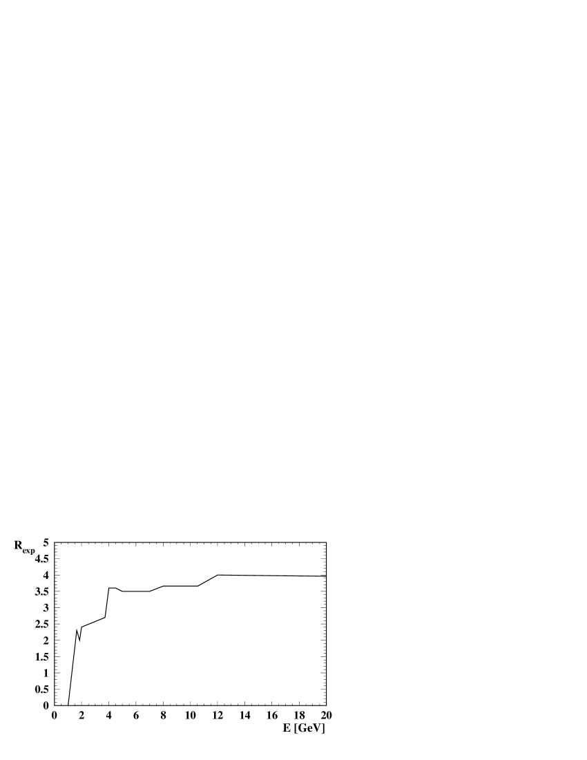
Figure 2: Parametrisation of $R(s)$ in the threshold region, without resonances, as provided by [5].

A convenient approach adopted to the experimental procedures is to decompose the final states into continuum (Fig.2) and resonance contributions. For the continuum one finds

$$R(\infty)=11/3\,,\ R_{0}=-13.240\,,\ R_{1}=20.875\,,\ R_{2}=-3.587\,.$$ (11)

For the two pion ($\widehat{=}\rho$) contribution the parametrisation derived in [6] (set 1) is employed which leads to the following moments:

$$R(\infty)=0\,,\ R_{0}=4.319\,,\ R_{1}=-8.422\,,\ R_{2}=8.547\,.$$ (12)

For the remaining resonances the narrow width approximation can be applied

$$R(s)=\frac{9\pi\Gamma_{e^{+}e^{-}}M_{R}}{\alpha^{2}}\delta(s-M_{R}^{2})\,.$$ (13)

The input parameters are listed in table 1, together with the predicted relative rate.

Table 1: Input parameters used for the narrow resonances and relative rates of hadronic radiation.

Channel	$\Gamma_{e^{+}e^{-}}\ [{\rm keV}]$	$M\ [{\rm MeV}]$	Relative Rate
$2\pi$			$2.55\times 10^{-4}$
Continuum			$2.86\times 10^{-4}$
$\omega$	$0.60$	$781.95$	$2.34\times 10^{-5}$
$\phi$	$1.37$	$1019.41$	$3.56\times 10^{-5}$
$\psi$	$5.36$	$3096.93$	$2.25\times 10^{-5}$
$\psi^{\prime}$	$2.14$	$3686.00$	$6.55\times 10^{-6}$
$\Upsilon$	$1.34$	$9460.32$	$5.85\times 10^{-7}$

In total we find the following result

$$\frac{\Gamma_{l\bar{l}had}}{\Gamma_{l\bar{l}}}=6.30\times 10^{-4}\,.$$ (14)

Table 2: Contributions of different energy ranges to the relative rate $\Gamma_{l\bar{l}had}/\Gamma_{l\bar{l}}$.

Energy range	Contribution to $\Gamma_{l\bar{l}had}/\Gamma_{l\bar{l}}$
$0\leq m_{had}\leq 2$ GeV	$3.88\times 10^{-4}$
$2\ {\rm GeV}\leq m_{had}\leq 3$ GeV	$5.87\times 10^{-5}$
$3\ {\rm GeV}\leq m_{had}\leq 10$ GeV	$1.52\times 10^{-4}$
$10\ {\rm GeV}\leq m_{had}\leq M_{Z}$	$3.16\times 10^{-5}$

It should be reiterated that this contribution corresponds to configurations where the invariant mass of the lepton pair is typically large and the mass of the hadronic system small. This is evident from table 2 where the contribution for $m_{had}\geq 10\ {\rm GeV}$ is also shown separately.
The numbers listed in tables 1 and 2 are difficult to compare with those from [3]. There the calculation was performed numerically for a $q\bar{q}l\bar{l}$ final state with a fixed quark mass of $300$ MeV. For $l=e$ and to lesser extend for $l=\mu$ their result is necessarily dominated by final states with large hadronic mass, that is a multi–hadron final state plus a lepton pair of low invariant mass. It seems experimentally difficult to isolate these events among the multi–hadron states, which occur with a relative rate below $10^{-3}$. It is however an interesting exercise to apply (9) and the formulas discussed below to $l\bar{l}q\bar{q}$ production where again the hadrons are radiated off the lepton. These can experimentally isolated by considering events with large invariant mass of the lepton pair. Adopting the quark mass values of [3], viz. $m_{u}=m_{d}=m_{s}=300\ {\rm MeV}$, $m_{c}=1.5\ {\rm GeV}$ and $m_{b}=4.5\ {\rm GeV}$ one predicts

$$\frac{\Gamma_{l\bar{l}u\bar{u}}}{\Gamma_{l\bar{l}}} = 4\frac{\Gamma_{l\bar{l}d\bar{d}}}{\Gamma_{l\bar{l}}}=4\frac{\Gamma_{l\bar{l}s\bar{s}}}{\Gamma_{l\bar{l}}}=2.256\times 10^{-4}\,,$$

$$\frac{\Gamma_{l\bar{l}c\bar{c}}}{\Gamma_{l\bar{l}}} = 5.259\times 10^{-5}\,,$$

$$\frac{\Gamma_{l\bar{l}b\bar{b}}}{\Gamma_{l\bar{l}}} = 2.858\times 10^{-6}\,,$$

$$\frac{\Gamma_{l\bar{l}had}}{\Gamma_{l\bar{l}}} = 3.938\times 10^{-4}\,.$$ (15)

We find that this model which has been used in [3], underestimates the rate for radiation by a factor $0.63$. An experimental analysis based on this model could, therefore, lead to drastically wrong conclusions. The reason for the discrepancy is fairly evident: The events are dominated by hadronic states with low invariant mass, where the parton model provides a poor approximation. This is reflected in a strong sensitivity of the results towards the choice for $m_{q}$.
Four lepton final states. The same formalism can also be applied to purely leptonic final states, using the analytical results for the moments [4]

$$R(\infty) = 1\,,\quad R_{0}=\ln 4-\frac{5}{3}\,,$$

$$R_{1} = \frac{1}{2}\ln^{2}4-\frac{5}{3}\ln 4+\left[\frac{28}{9}-\zeta_{2}\right]\,,$$

$$R_{2} = \frac{1}{6}\ln^{3}4-\frac{5}{6}\ln^{2}4+\left[\frac{28}{9}-\zeta_{2}\right]\ln 4+2\zeta_{3}+\frac{5}{3}\zeta_{2}-\frac{164}{27}\,.$$ (16)

The numerical results for $\Gamma_{e^{+}e^{-}l\bar{l}}/\Gamma_{e^{+}e^{-}}$ are $3.319\times 10^{-4}$ for $l=\mu$ and $3.214\times 10^{-5}$ for $l=\tau$. It should be reiterated that this result refers to final states where the $l\bar{l}$ is radiated off the $e^{+}e^{-}$ pair and hence is dominated by $l\bar{l}$ with low invariant mass. Eq.9 can be also used to predict the rate for lepton pair radiation if a cut $s_{l^{+}l^{-}}>s_{0}\gg 4m_{l}^{2}$ is employed. In this case one may simply put $R_{0}=R_{1}=R_{2}=0$ and $y=s/s_{0}$ . Characteristical examples are $\Gamma_{e^{+}e^{-}l^{+}l^{-}}/\Gamma_{e^{+}e^{-}}=5.321\times 10^{-4}/1.268\times 10^{-4}/8.716\times 10^{-6}$ for $\sqrt{s_{0}}=0.1/1/10\ {\rm GeV}$ respectively.

Secondary radiation of heavy quarks. Replacing the factor $(\alpha/\pi)^{2}$ by $(\alpha_{s}/\pi)^{2}\,2/3$, the perturbative result of eq.9 combined with eq.16 can be applied to predict the rate for secondary production of heavy quarks in $Z\to q\bar{q}$ events, where $q$ denotes a light quark. For $m_{b}=4.5/4.8/5.0$ GeV one predicts a relative rate of $1.545\times 10^{-3}/1.391\times 10^{-3}/1.301\times 10^{-3}$. The corresponding numbers for secondary charm production $(m_{c}=1.3/1.5/1.8\ {\rm GeV})$ are significantly larger and amount to $8.339\times 10^{-3}/7.107\times 10^{-3}/5.729\times 10^{-3}$ respectively. These rates should be well observable with present day statistics.

Combination with virtual corrections. The third and second power of the logarithm of $y$ cancel after combining real radiation of hadrons (or leptons) with the corresponding virtual corrections to the form factor [4]

$${\rm Re}F^{(4)} = R(\infty)\left\{-\frac{1}{36}\ln^{3}y+\frac{1}{8}\ln^{2}y+\left[\frac{1}{6}\zeta_{2}-\frac{7}{24}\right]\ln y-\frac{1}{4}\zeta_{2}+\frac{5}{16}\right\}+$$ (17)

$$R_{0}\left[-\frac{1}{12}\ln^{2}y+\frac{1}{4}\ln y+\frac{1}{6}\zeta_{2}-\frac{7}{24}\right]+R_{1}\left(-\frac{1}{6}\ln y+\frac{1}{4}\right)-\frac{1}{6}R_{2}\,,$$

and one obtains for the correction to the total rate

$$\frac{\delta\Gamma^{(4)}}{\Gamma} = 2\left(\frac{\alpha}{\pi}\right)^{2}{\rm Re}F^{(4)}+\frac{\Gamma_{e^{+}e^{-}l\bar{l}}}{\Gamma_{e^{+}e^{-}}}$$ (18)

$$= \left(\frac{\alpha}{\pi}\right)^{2}\left\{R(\infty)\left[\frac{1}{4}\ln y-\frac{23}{24}+\zeta_{3}\right]+\frac{1}{4}R_{0}\right\}\,.$$

The coefficient of the remaining logarithm can be easily understood: The lowest order correction (from real and virtual photon radiation) is given by a factor $(1+\frac{3}{4}\frac{\alpha}{\pi})$. The fine structure constant $\alpha$ can be replaced by the running $\alpha(s)=\alpha/(1-\Pi(s))$. The vacuum polarisation from hadronic (or leptonic) intermediate states can be expressed in terms of $R$ through

$${\rm Re}\Pi(s) = \frac{\alpha}{\pi}\frac{s}{3}\int_{4\mu^{2}}^{\infty}\frac{{\rm d}s^{\prime}}{s^{\prime}}\frac{R(s^{\prime})}{s-s^{\prime}}$$ (19)

$$\approx \frac{\alpha}{\pi}\left(\frac{1}{3}R(\infty)\ln\frac{s}{4\mu^{2}}+\frac{1}{3}R_{0}\right)\,,$$

and one obtains for the complete correction (without ${\cal O}(\alpha^{2})$ photonic terms)

$$1+\frac{3}{4}\frac{\alpha(s)}{\pi}+\frac{1}{6}\left(\frac{\alpha}{\pi}\right)^{2}\left(6\zeta_{3}-\frac{23}{4}\right)\,.$$ (20)

An amusing test of (18), combined with the moments from (16), is provided by the results of [1]. If one replaces the $SU(3)$ factors in this paper by the corresponding abelian coefficients, and, furthermore, relates the $\overline{MS}$ coupling $\alpha_{\overline{MS}}$ to the conventionally defined fine structure constant

$${\overline{\alpha}}=\alpha\left(1+\alpha\frac{1}{3}\ln\frac{\mu^{2}}{m^{2}}\right)$$ (21)

one obtains agreement between the two results.

References

References

[1] K.G. Chetyrkin, A.L. Kataev and F.V. Thachov,
Phys. Lett. B 85 (1979) 277
[2] B.A. Kniehl and J.H. Kühn, Nucl. Phys. B 329 (1990) 547
[3] E.W.N. Glover, R. Kleiss and J. van der Bij,
Z. Phys. C 47 (1990) 435 and refs. therein
[4] B.A. Kniehl, M. Krawczyk, J.H. Kühn and
R.G. Stuart, Phys. Lett. B 209 (1988) 337
[5] H. Burkhardt, Radiative Corrections, edited by
N. Dombey and F. Boudjema, Plenum Press, New York, 1990;
H. Burkhardt, privat communication
[6] J.H. Kühn and A. Santamaria, Z. Phys. C 48 (1990) 449