$\bar{p}p$ partial-wave analysis and
$\overline{N}\!N$ potentials

Abstract

A review is given of the different ways to describe $\bar{p}p$ scattering. Next the Nijmegen partial-wave analyses of the $\bar{p}p$ data as well as the corresponding Nijmegen $\overline{N}\!N$ database are discussed. These partial-wave analyses are finally used as a tool to construct a better $\overline{N}\!N$ potential model and also to clarify questions raised in the literature.

1 Introduction

Starting with an antiproton beam directed on a proton target many reactions are possible. First of all is the elastic scattering $\bar{p}p\rightarrow\bar{p}p$. For this reaction differential cross sections $\sigma_{el}(\theta)$, analyzing-power data $A_{el}(\theta)$ [1, 2], and even some depolarization data $D_{yy}(\theta)$ [3] have been measured. We will discuss these extensively in this talk. The annihilation channel, $\bar{p}p\rightarrow$ mesons, is studied very intensively by theorists as well as by experimentalists. Many different reactions can be distinguished. For our purposes, however, only a global description will turn out to be sufficient. The charge-exchange reaction $\bar{p}p\rightarrow\bar{n}n$ has its threshold at $p_{L}=99$ MeV/c. Important is that in the one-boson-exchange (OBE) picture only charged mesons can be exchanged. The most important of these are the $\pi^{\pm}$ and $\rho^{\pm}$ mesons. The study of this reaction allowed us to determine the coupling constant of the charged pion to the nucleons [4]. Recently, excellent data for this charge-exchange reaction has been obtained at LEAR for the differential cross section $\sigma_{ce}(\theta)$ and for the analyzing power $A_{ce}(\theta)$ [5]. Very recently, even charge-exchange depolarization data have become available [6]. Excellent data are also available for the strangeness-exchange reaction $\bar{p}p\rightarrow\bar{\Lambda}\Lambda$ with threshold $p_{L}=1.435$ GeV/c [7]. More data for this reaction are forthcoming as well as data for the other strangeness-exchange reactions $\bar{p}p\rightarrow\bar{\Lambda}\Sigma,\bar{\Sigma}\Lambda$ [8] and $\bar{\Sigma}\Sigma$. These reactions are very important for the precise determination of the $\Lambda N\!K$ and $\Sigma N\!K$ coupling constants and combining these with the $N\!N\pi$ coupling constant gives us information about flavor SU(3) [9].

2 Antinucleon-nucleon potentials

It is customary to start with some meson-theoretic $N\!N$ potential and then apply the $G$-parity transformation [10] to get the corresponding $\overline{N}\!N$ potential. This is a straightforward, but rather cumbersome procedure. When you ask people about details, then most people must confess that they do not know.

We would like to point out that just charge conjugation, together with charge independence, without actually combining them to $G$, is sufficient for our purposes. To understand this, let us look at the $ppm^{0}$ vertex describing the coupling of a neutral meson $m^{0}$ to the proton $p$ with a coupling constant $g$. When we apply charge conjugation $C$ we have

$$\bar{p}=Cp\rule{28.45274pt}{0.0pt}{\rm and}\rule{28.45274pt}{0.0pt}\overline{m^{0}}=Cm^{0}\ ,$$

and we describe now the $\bar{p}\bar{p}\overline{m^{0}}$ vertex. For nonstrange, neutral mesons $m^{0}$ one can define the charge parity $\eta_{c}$ by $\overline{m^{0}}=\eta_{c}m^{0}$. Charge-conjugation invariance of the interaction Lagrangian describing this $ppm^{0}$ vertex requires that the coupling constant $g$ of the meson $m^{0}$ to the proton $p$ is equal to the coupling constant of the antimeson $\overline{m^{0}}$ to the antiproton $\bar{p}$. The coupling constant $\bar{g}$ of the meson $m^{0}$ to the antiproton is then given by

$$\bar{g}=\eta_{c}g\ .$$

For mesons of the type $Q\overline{Q}$, with relative orbital angular momentum $L$ and total spin $S$ the charge parity is

$$\eta_{c}=(-)^{L+S}\ .$$

Therefore the pseudoscalar (${}^{1}S_{0}$) mesons have $J^{PC}=0^{-+}$, the vector (${}^{3}S_{1}$) mesons have $J^{PC}=1^{--}$, the scalar (${}^{3}P_{0}$) mesons have $J^{PC}=0^{++}$, etc.

We see that from the important mesons only the vector mesons have negative charge parity and therefore the coupling constants of the vector mesons change sign when going from the nucleons to the antinucleons. In the OBE picture the $pp$ potential $V(pp)$ is the sum of the exchanges of the pseudoscalar meson $\pi$, the vector mesons $\rho$ and $\omega$, the scalar meson $\varepsilon(760)$, etc. That is

$$V(pp)=V_{\pi}+V_{\rho}+V_{\omega}+V_{\varepsilon}+\ldots$$

The potential $V(\bar{p}p)$ described in the same OBE picture is then given by

$$V(\bar{p}p)=V_{\pi}-V_{\rho}-V_{\omega}+V_{\varepsilon}+\ldots$$

In these reactions only neutral mesons are exchanged. When we want to describe the charge-exchange reaction $\bar{p}p\rightarrow\bar{n}n$, then it is easiest to recall charge independence. Charge independence requires that the coupling constant $g_{c}$ of the charged meson to the nucleons is given by $g_{c}=g\sqrt{2}$, and to the antinucleons by $\bar{g}_{c}=\bar{g}\sqrt{2}$. The charge-exchange potential is therefore given by

$$V_{ce}=2(V_{\pi}-V_{\rho}+\ldots)\ .$$

The diagonal potential in the $\bar{n}n$ channel is, using charge independence, given by $V(\bar{n}n)=V(\bar{p}p)$.

What can we learn from the $N\!N$ potentials about the $\overline{N}\!N$ potentials?
The $pp$ central force is relatively weak due to the cancellations between the repulsive contribution of the vector mesons $\omega$ and $\rho$ and the attractive contribution of the scalar mesons $\varepsilon(760)$, etc. The $\bar{p}p$ central force is strongly attractive, because the vectors mesons have now an attractive contribution which adds coherently to the attractive contribution of the scalar mesons, giving a very strong overall central force. Also the tensor force in $N\!N$ is relatively weak, because $\pi$ and the important $\rho$ contributions have opposite sign. In the $\overline{N}\!N$ case these mesons add coherently again to give a very strong tensor force. This strong tensor force is responsible for the importance of the transitions

$$\ {}^{3}S_{1}\leftrightarrow\ ^{3}D_{1}\rule{28.45274pt}{0.0pt},\rule{28.45274pt}{0.0pt}\ ^{3}P_{2}\leftrightarrow\ ^{3}F_{2}\rule{28.45274pt}{0.0pt},\rule{28.45274pt}{0.0pt}\ ^{3}D_{3}\leftrightarrow\ ^{3}G_{3}\rule{28.45274pt}{0.0pt}{\rm etc.}$$

3 Various models

3.1 Black-disk model

One of the simplest models for the description of the elastic and inelastic cross section is the black-disk model. This model gives

$$\sigma_{el}=\sigma_{ann}=\frac{1}{2}\sigma_{T}=\pi R^{2}\ ,$$

where $R$ is the radius of the black disk. This relation is satisfied very approximately. It shows that the annihilation cross section predicts radii for the black disk which are energy dependent and pretty large. In the momentum interval 200 MeV/c $<p_{L}<$ 1 GeV/c this radius $R$ varies from more than 2 fm to about 1.4 fm.

3.2 Boundary-condition model

The boundary-condition model in $\overline{N}\!N$ was first introduced by M. Spergel in 1967 [11]. Later many more people used this now more than a quarter century old model (see e.g. Refs. [12, 13]). The model is based on the observation that the interaction for large values of the radius is often well-known, while the interaction for small radii is very hard to describe. This problem is then solved by just specifying a boundary condition at $r=b$. For this boundary condition one takes the logarithmic derivative of the radial wave function at the boundary radius $b$

$$P=b\left(\frac{d\psi}{dr}/\psi\right)_{r=b}\ .$$

Outside this radius one assumes that the interaction can be described by a known potential $V_{L}$. This long-range interaction is made of meson exchanges as described in section 2 and it contains of course also the electromagnetic interaction.

A nice, instructive example is the modified black disk, where $V_{L}=0$ and $P=-ipb$. The $P$ matrix contains a negative imaginary part, implying absorption of flux at the boundary. The boundary $b$ is a measure for the annihilation radius. This modified black disk is specified by only one parameter: the radius $b$.

When one looks how these boundary-condition models have been used, then one sees that in these extremely simple models every time only very few parameters have been introduced. The conclusion is that such a few-parameter model can fit possibly some data, but it will never be able to fit all the available $\overline{N}\!N$ data, with the same set of only a few parameters.

3.3 Optical-potential model

The optical-potential models have become quite an industry in the $\overline{N}\!N$ community. The first such model was from R. Bryan and R. Phillips in 1968 [14]. In the optical-potential model the interaction between the antinucleon and the nucleon is described by a complex potential from $r=0$ to infinity. For the basic potential one takes a meson-theoretic potential, obtained from some known $N\!N$ potential by using the charge-conjugation operation. Then, in order to get annihilation, to this potential is added another complex potential,

$$V(r)=(U-iW)f(r)\ .$$

Here $U$ and $W$ are constants and $f(r)$ is some radial function. This radial function can be the Woods-Saxon form, a Gaussian form, or even a square well. Let us give you a DO-IT-YOURSELF-KIT called:

How to make your own optical potential?

Instructions:
1. Look through the literature and decide which $N\!N$ potential your want to use.
2. Apply to this potential charge conjugation, so that you obtain the corresponding $\overline{N}\!N$ potential.
3. Pick your favored functional form for $f(r)$. This will contain a range parameter $b$. After you have made this choice, find some arguments, which sound like QCD, to justify this chosen form.
4. Pick one of the beautiful differential cross sections as measured by Eisenhandler et al. [15] and adjust $U$, $W$, and $b$ such that a reasonable fit (at least at sight) is obtained for this particular cross section.
Your model is now a three-parameter model, which fits some of the data (at least the Eisenhandler data at one energy) reasonably well (at sight), but it cannot possibly fit all the $\overline{N}\!N$ data, because the model does not have enough freedom.

After Bryan and Phillips many people have constructed similar models (see e.g. Refs. [16, 17, 18, 19]). Also in Nijmegen we made such an optical-potential model, which we optimized by making a least-squares fit to our database, which contained at that time $N_{d}=3309$ data. Because we actually performed a fit to all the $\overline{N}\!N$ data we think that we will have about the lowest $\chi^{2}$ of all the available two- or three-parameter optical-potential models. For our model $\chi_{\rm min}^{2}=6\ 10^{9}$. This enormously large number is NOT a printing error, but just an expression of the total failure of such simple models. It is, therefore, astonishing to see that regularly new measurements from LEAR are compared to one or more of these few-parameter optical-potential models (see e.g. Ref. [3]), as if something can be learned from such a comparison!

There is only one group, the theory group of R. Vinh Mau in Paris, that has seriously tried to fit all available $\overline{N}\!N$ data with an optical-potential model. In 1982 they got a fit with $\chi^{2}/N_{d}=2.8$, where they compared with the then available pre-LEAR data [20]. In 1991 they published an update [21], where they fitted now also the LEAR data. For the real part of the potential they took the $G$-conjugated Paris $N\!N$ potential [22]. Because the inner region of this $N\!N$ potential is treated totally phenomenologically it is impossible to take that over to $\overline{N}\!N$, so something has been done there and probably some extra parameters have been introduced. The imaginary part of the potential they write as

$$W(r) = \left\{\rule{0.0pt}{17.07164pt}g_{c}(1+f_{c}T_{L})+g_{ss}(1+f_{ss}T_{L})\,\mbox{\boldmath$\sigma$}_{1}\cdot\mbox{\boldmath$\sigma$}_{2}\right.$$

$$\left.+\,g_{T}S_{12}+g_{LS}\ {\bf L}\cdot{\bf S}\ \frac{1}{4m^{2}r}\frac{d}{dr}\right\}\frac{K_{0}(2mr)}{r}\ ,$$

where $T_{L}$ is the lab kinetic energy and the parameters are the $g$’s and the $f$’s. For each isospin a set of 6 parameters is fitted, so that the imaginary part is described by about 12 real parameters. In total the Paris $\overline{N}\!N$ potential uses at least 12, possibly about 22, parameters. The correct number used is not so important, what is important, is that the number is much larger than 3. The Paris group do fit then to 2714 data and get $\chi^{2}/N_{d}=6.7$. The quality of this fit is very hard to assess, because the Paris group did not try to make their own selection of the data, but tried to fit all the available data, many of which are contradictory. It would be interesting to see their fit to the Nijmegen $\bar{p}p$ database [30] (see section 5), where all the contradictory sets have been removed.

An important lesson could have been learned already in 1982 from this Paris work. An optical-potential model needs at least about 15 parameters to be able to give a reasonable fit to the $\overline{N}\!N$ data. This means that practically all few-parameter optical-potential models published after 1982 should have been rejected by the journals.

3.4 Coupled-channels model

Another way to introduce inelasticity in our formalism is to introduce explicitly couplings from the $\overline{N}\!N$ channels to annihilation channels. This was done in 1984 by P. Timmers et al. in the Nijmegen coupled-channels model: CC84 [23]. Fitting to the then available pre-LEAR data resulted in a quite satisfactory fit with $\chi^{2}/N_{d}=1.39$. Several people have have later tried similar models [24, 25]. An update of the old model CC84 was made in 1991 in Nijmegen in the thesis of R. Timmermans [26]. This new coupled-channels model, which we would like to call the Nijmegen model CC93, gives $\chi^{2}/N_{d}=1.58$, when fitted to $N_{d}=3646$ data. We will come back to this model somewhat later.

4 Antiproton-proton partial-wave analysis

In Nijmegen we have for almost 15 years been busy with partial-wave analyses of the $N\!N$ data. We have now developed rather sophisticated and accurate methods to do these PWA’s [27, 28, 29]. A few years ago we realized that it was possible to do a PWA of all the available $\bar{p}p$ data in exactly the same way as our $N\!N$ PWA. Before this realization we always thought that such a PWA would be almost impossible in $\overline{N}\!N$. Luckily, it is not impossible. We will try to give a short description of our PWA [30].

In an energy-dependent partial-wave analysis one needs a model to describe the energy dependence of the various partial-wave amplitudes. Our model is a mixture of the boundary-condition model and the optical-potential model. We choose the boundary at $b=1.3$ fm. This value is determined by the width of the diffraction peak and cannot be chosen differently, without deteriorating the fit to the data. The long-range potential $V_{L}$ for $r>b$ is

$$V_{L}=V_{\overline{N}\!N}+V_{C}+V_{M\!M}\ .$$

Here $V_{C}$ is the relativistic Coulomb potential, $V_{M\!M}$ the magnetic-moment interaction, and $V_{\overline{N}\!N}$ is the charge-conjugated Nijmegen $N\!N$ potential, Nijm78 [31]. We solve the relativistic Schrödinger equation [32] for each energy and for each partial wave, subject to the boundary condition

$$P=b\left(\frac{d\psi}{dr}/\psi\right)_{r=b}\ ,$$

at $r=b$. This boundary condition may be energy dependent. To get the value of $P$ as a function of the energy we use for the spin-uncoupled waves (like ${}^{1}S_{0}$, ${}^{1}P_{1}$, ${}^{1}D_{2}$, $\ldots$ and ${}^{3}P_{0}$, ${}^{3}P_{1}$, ${}^{3}D_{2}$, $\ldots$) the optical-potential picture. We take a square-well optical potential for $r\leq b$. This short-ranged potential $V_{S}$ we write as

$$V_{S}=U_{S}-iW_{S}\ .$$

In this way we get in each partial wave and for each isospin the parameters $U_{S}$ and $W_{S}$. Using these potentials we can calculate easily the boundary condition $P$ and the scattering amplitudes. For example in all singlet waves ${}^{1}S_{0}$, ${}^{1}P_{1}$, ${}^{1}D_{2}$, $\ldots$, we get $U=0$ and $W\approx 100$ MeV. For the triplet waves we take $W$ independent of the isospin. The parameters for the ${}^{3}P_{0}$ wave are e.g. $W=159\pm 9$ MeV and independent of the isospin, and $U(I=0)=-132\pm 9$ MeV and $U(I=1)=178\pm 19$ MeV. To describe all relevant partial waves we need in our $\overline{N}\!N$ PWA 30 parameters. In our fit to the data we use all available data in the momentum interval 119 MeV/c $<p_{L}<$ 923 MeV/c. The lowest momentum is determined by the fact that for lower momenta no data are available. The highest momentum is determined by several considerations. In $N\!N$ we use all data up to $T_{L}=350$ MeV, which corresponds to $p_{L}=810$ MeV/c. Because we wanted to include all the elastic backward cross sections of Alston-Garnjost et al. [33], we need to go to $p_{L}=923$ MeV/c which corresponds to $T_{L}=454$ MeV. At this energy the potential description in $N\!N$ is still valid, and therefore we feel that also here our description must work at least up to this momentum.

Our final dataset contains $N_{d}=3646$ experimental data. In our analyses we need to determine $N_{n}=113$ normalizations and $N_{p}=30$ parameters. This leads to the number $N_{df}$ of degrees of freedom $N_{df}=N_{d}-N_{n}-N_{p}=3503$. When the dataset is a perfect statistical ensemble and when the model to describe the data is totally correct, then one expects for $\chi^{2}_{\rm min}$:

$$\langle\chi^{2}_{\rm min}\rangle=N_{df}\pm\sqrt{2N_{df}}\ .$$

Thus expected is $\langle\chi^{2}_{\rm min}(\bar{p}p)\rangle/N_{df}=1.000\pm.024$.
In our PWA we obtain $\chi^{2}_{\rm min}(\bar{p}p)/N_{df}=1.085$. We see that we are about 3.5 standard deviations away from the expectation value. To get a feeling for these numbers let us compare with the $pp$ data and the $pp$ PWA. The number of data is now $N_{d}=1787$ and we expect

$$\langle\chi^{2}_{\rm min}(pp)\rangle/N_{df}=1.000\pm 0.035\ .$$

In the latest Nijmegen analysis, NijmPWA93 [29], we get

$$\chi^{2}_{\rm min}(pp)/N_{df}=1.108,$$

which is 3 standard deviations too high. We see that our $\bar{p}p$ analysis compares favorable with a similar analysis for the $pp$ data. This means therefore that we have a statistically rather good solution and also that this solution will be essentially correct.

5 The Nijmegen ${\bf\overline{N}\!N}$ database

An essential ingredient in our successfully completed PWA, as well as an important product of this PWA, is the Nijmegen $\overline{N}\!N$ database [30]. As pointed out before, we use all data with $p_{L}<925$ MeV/c or $T_{L}<454$ MeV. This means that our momentum range is similar to the momentum range used in the Nijmegen $N\!N$ PWA’s. We will compare regularly with the $N\!N$ case to show that the same methods, which work well in $N\!N$, work also well in $\overline{N}\!N$ and that the results are also similar.

The number of data $N_{d}$ in the various final datasets are $N_{d}(\bar{p}p)=3543$, $N_{d}(pp)=1787$, and $N_{d}(np)=2514$. In the processes to come to these final datasets we had to reject data. We do not want to go into details [27] about what are the various criteria to remove data from the dataset. We would like to point out, however, that in $pp$ scattering there is a long history about which datasets are reliable, and which not. We did not invent the method of discarding incorrect data, we just followed common practice and used common sense. In the $\bar{p}p$ case we needed to reject 744 data, which is 17% of our final dataset. In the $pp$ case we discarded 292 data or 14% of the final dataset, and in the $np$ case we rejected 932 data, which amounts to 27% of the final dataset. It is clear that the $\bar{p}p$ case does not seem to be out of bounds. Of course, it is unfortunate that so many data have to be rejected, because these data represented many man-years of work and a lot of money and effort. However, when one wants to treat the data in a statistically correct manner, then often one cannot handle all datasets, but one must reject certain datasets. This does not mean that all these rejected datasets are “bad” data, it only means, that if we want to apply statistical methods, then, unfortunately, certain datasets cannot be used.

	elastic		charge exchange
	LEAR	rest	LEAR	rest
$\sigma_{T},\sigma_{A}$	124	-	-	63
$\sigma(\theta)$	281	2507	91	154
$A(\theta)$	200	29	89	-
$D$	5	-	9	-
total	610	2536	189	217

Table 1: Number of elastic and charge-exchange data divided over various categories.

In Table 1 we give the number of data points divided into elastic versus charge exchange, LEAR versus the rest, and total cross sections $\sigma_{T}$, annihilation cross sections $\sigma_{A}$, differential cross sections $\sigma(\theta)$, analyzing-power data $A(\theta)$, and depolarization data $D(\theta)$. This table give some interesting information.
The most striking fact is that:
Of the final dataset only $22$% of the data comes from LEAR.
This is after 10 years operation of LEAR. Remember the promises (or were it boasts) from CERN, made before LEAR was built. They were something like: “Only one day running of LEAR will produce more scattering data then all other methods together.” Unfortunately, this promise of CERN did not work out. Also it is clear that LEAR has not given much valuable information about $\sigma(\theta)$ for the elastic reaction. A lot of the elastic $\sigma(\theta)$ data from LEAR unfortunately needed to be rejected [30]! This does not mean that LEAR did not produce beautiful data. Some of the charge-exchange data and the strangeness-exchange data are really of high quality.

Another striking fact is the virtual absence of spin-transfer and spin-correlation data. For the elastic reaction below 925 MeV/c there are only 5 depolarizations measured with enormous errors [3]. Very recently, some depolarization data of good quality have become available for the charge-exchange reaction [6].

A valid question is therefore:
Can one do a PWA of the $\bar{p}p$ data, when there are essentially no “spin data”?
The answer is yes! The proof that it can be done lies in the fact that we actually produced a $\bar{p}p$ PWA with a very good $\chi^{2}/N_{d}$. We have also checked this at length in our $pp$ PWA’s. We convinced ourselves that a $pp$ PWA using only $\sigma(\theta)$ and $A(\theta)$ data gives a pretty good solution. Of course, adding spin-transfer and spin-correlation data was helpful and tightened the error bands. However, most spin-transfer and spin-correlation data in the $pp$ dataset actually did not give any additional information.

6 Fits to the data

It is of course impossible to show here how well the various experimental data are fitted. From our final $\chi^{2}/N_{d}=1.085$ one can draw the conclusion, that almost every dataset will have a contribution to $\chi^{2}$ which is roughly equal to the number of data points as is required by statistics. Let us look at some of the experimental data. In Fig. 1 we present total cross sections from PS172 [34]. The fit gives for these 75 data points $\chi^{2}=88.4$. In the same Fig. 1 one can also find 52 annihilation cross sections from PS173 [35]. These points contributed $\chi^{2}=65.3$ to the total $\chi^{2}$.

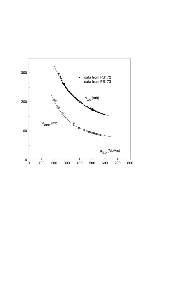
Figure 1: Total cross sections (PS172) and annihilation cross sections (PS173) with the curves from the Nijmegen PWA.

In Fig. 2 we plot the elastic differential cross section $\sigma(\theta)$ at $p_{L}=790$ MeV/c as measured in 1976 by Eisenhandler et al. [15] The 95 data points contribute $\chi^{2}=101.5$. The vertical scale is logarithmic. The nice fit reflects the high quality of these pre-LEAR data.

Figure 2: Elastic differential cross section at 790 MeV/c from Eisenhandler et al., with the curve from the Nijmegen PWA.

The differential cross section of the charge-exchange reaction $\bar{p}p\rightarrow\bar{n}n$ at $p_{L}=693$ MeV/c as measured by PS199 is given in Fig. 3. The 33 data contribute $\chi^{2}=39.3$. This dataset can be considered important, because it is very constraining. One needs all partial waves up to $L=10$ to get a satisfactory fit to these data.

Figure 3: Charge-exchange differential cross section at 693 MeV/c from PS199, with the curve from the Nijmegen PWA.

7 Coupled-channels potential model

Having finished our discussion of the Nijmegen $\bar{p}p$ partial-wave analysis we can look at the $\overline{N}\!N$ potentials. We decided to update the old coupled-channels model Nijmegen CC84 of Timmers et al. [23]. Because of our experience with the various datasets this was not very difficult, just very computer-time consuming. The result was the new Nijmegen CC93 model [26]. In this model we treat the $\overline{N}\!N$ coupled channels on the particle basis. We therefore have a $\bar{p}p$ channel as well as a $\bar{n}n$ channel. This allows us to introduce the charge-independence breaking effects of the Coulomb interaction in the $\bar{p}p$ channel and of the mass differences between the proton and neutron as well as between the exchanged $\pi^{0}$ and $\pi^{\pm}$.

These $\overline{N}\!N$ channels are coupled to annihilation channels. We assume here that annihilation can happen only into two fictitious mesons; into one pair of mesons with total mass 1700 MeV/c², and into another pair with total mass 700 MeV/c². Moreover, we assume that these annihilation channels appear in both isospins $I=0$ as well as $I=1$. We end up with 6 coupled channels for each of the $\bar{p}p$ channels: ${}^{1}S_{0}$, ${}^{1}P_{1}$, ${}^{1}D_{2}$, ${}^{1}F_{3}$, etc. and ${}^{3}P_{0}$, ${}^{3}P_{1}$, ${}^{3}D_{2}$, ${}^{3}F_{3}$, etc. Due to the tensor force we end up with 12 coupled channels for each of the $\bar{p}p$ coupled channels: ${}^{3}S_{1}+\,^{3}D_{1}$, ${}^{3}P_{2}+\,^{3}F_{2}$, ${}^{3}D_{3}+\,^{3}G_{3}$, etc.

We use the relativistic Schrödinger equation in coordinate space. The interaction is then described by either a $6\times 6$ or a $12\times 12$ potential matrix

$$V=\left(\begin{array}[]{cc}V_{\overline{N}\!N}&V_{\!A}\\[5.69054pt] \widetilde{V}_{\!A}&0\end{array}\right)\ .$$

The $2\times 2$ (or $4\times 4$) submatrix $V_{\overline{N}\!N}$ we write as

$$V_{\overline{N}\!N}=V_{C}+V_{M\!M}+V_{O\!B\!E}\ ,$$

where for $V_{C}$ we use the relativistic Coulomb potential, $V_{M\!M}$ describes the magnetic-moment interaction, and for $V_{O\!B\!E}$ we use the charge-conjugated Nijmegen $N\!N$ potential Nijm78 [31]. We have assumed that we may neglect the diagonal interaction in the annihilation channels. The annihilation potential $V_{\!A}$ connects the $\overline{N}\!N$ channels to the two-meson annihilation channels. It is either a $2\times 4$ matrix or a $4\times 8$ matrix. This potential we write as

$$V_{\!A}(r)=\left(V_{C}+V_{SS}\mbox{\boldmath$\sigma$}_{1}\cdot\mbox{\boldmath$\sigma$}_{2}+V_{T}S_{12}m_{a}r+V_{SO}{\bf L}\cdot{\bf S}\frac{1}{m_{a}^{2}r}\frac{d}{dr}\right)\frac{1}{1+e^{m_{a}r}}\ .$$

The factor $m_{a}r$ is introduced in the tensor force to make this potential identically zero at the origin. Here $m_{a}$ is the mass of the meson (either 850 MeV/c² or 350 MeV/c²). This annihilation potential depends on the spin structure of the initial state. For each isospin and for each meson channel five parameters are introduced: $V_{C}$, $V_{SS}$, $V_{T}$, $V_{SO}$, and $m_{a}$. This gives a model with in total $4\times 5=20$ parameters. These parameters can then be fitted to the $\overline{N}\!N$ data. Doing this we obtained $\chi^{2}/N_{d}=3.5$. It is clear, of course, that although the old Nijmegen soft-core potential Nijm78 is a pretty good $N\!N$ potential, it is definitely not the ultimate potential. We decided therefore to introduce now as extra parameters the coupling constants of the $\rho$, $\omega$, $\varepsilon(760)$, pomeron, and $a_{0}(980)$. Adding these parameters allowed us quite a drop in $\chi^{2}$. Now we reached

$$\chi^{2}/N_{d}=1.58\ ,$$

with a total of 26 parameters.

8 The reaction $\bar{p}p\rightarrow\bar{\Lambda}\Lambda$

It is perhaps not superfluous to point out here, that we also made a PWA of the strangeness-exchange reaction $\bar{p}p\rightarrow\bar{\Lambda}\Lambda$ [9, 36]. Fitting the $N_{d}=142$ data, we get $\chi^{2}_{\rm min}/N_{d}=1.027$.

The first theoretical treatments of this reaction were by F. Tabakin and R.A. Eisenstein [37] and independently by P. Timmers in his thesis [38]. Many other treatments of this reaction can be found (see e.g. Refs. [39, 40, 41, 42, 43, 44, 45]). In the meson-exchange models it is clear that next to $K(494)$ exchange, there is also the exchange of the vector meson $K^{*}(892)$. In Nijmegen we have been able to determine the $\Lambda N\!K$ coupling constant at the pole [9]. We found $f^{2}_{\Lambda N\!K}=0.071\pm 0.007$. This value is in agreement with the value $f^{2}_{\Lambda N\!K}=0.0734$ used in the recent soft-core Nijmegen hyperon-nucleon potential [46]. When we determine also the mass of the exchanged pseudoscalar meson we find $m(K)=480\pm 60$ MeV in good agreement with the experimental value $m(K)=493.646(9)$ MeV. This shows that we are actually looking at the one-kaon-exchange mechanism in the reaction $\bar{p}p\rightarrow\bar{\Lambda}\Lambda$.

When the data for the reactions $\bar{p}p\rightarrow\bar{\Lambda}\Sigma$ and $\bar{\Sigma}\Lambda$ are available, then also the $\Sigma N\!K$ coupling constant can be determined. When this can be done with sufficient accuracy, then information about the SU(3) ratio $\alpha=F/(F+D)$ can be obtained, and SU(3) for these coupling constants can then actually be studied.

9 PWA as a TOOL

We have presented here some of the results of the first, energy-dependent partial-wave analysis of the elastic and charge-exchange $\bar{p}p$ scattering data [30]. We also discussed the Nijmegen $\overline{N}\!N$ dataset, where we removed the contradictory or otherwise not so good data from the world $\bar{p}p$ dataset.

The main reason that we have been able to perform a PWA of the $\bar{p}p$ scattering data is that practically all partial-wave amplitudes are dominated by the potential outside $r=1.3$ fm. This long range potential consists of the electromagnetic potential, the OPE potential, and the exchange potentials of the mesons like $\rho,\ \omega,\ \varepsilon$, etc. This long-range potential is therefore well known. In our PWA of the $N\!N$ scattering data [29] it was noticed by us that the long-range potential in the $N\!N$ case dominated the $N\!N$ partial-wave scattering amplitudes. In the $\bar{p}p$ case the long-range potential is much stronger (see section 2), and the dominance in the $\bar{p}p$ case is therefore more marked. One could formulate this the following way. The important $\bar{p}p$ partial-wave amplitudes are “$\pi,\ \rho,\ \varepsilon$, and $\omega$ dominated.” This gives the most important energy dependence of these amplitudes. The slower energy dependence due to the short-range interaction can easily be parametrized.

A second reason for the successful PWA is the availability and easy access to computers, because the methods used are very computer intensive.

We want to stress the fact that our multienergy PWA can now be used as a tool. This tool allows us first of all to judge the quality of a particular dataset. This enabled to us to set up the Nijmegen $\overline{N}\!N$ database. Secondly, it can be used in the study of the $\overline{N}\!N$ interaction.

To demonstrate these things let us look at the Meeting Report of the Archamps meeting from October 1991 [47]. Beforehand the participants were asked to discuss at the meeting such questions as:
What is the evidence for one-pion exchange in the $\overline{N}\!N$ interaction?
In Nijmegen we determined [4, 30], using the PWA as a tool, the $N\!N\pi$ coupling constant for charged pions from the data of the charge-exchange reaction $\bar{p}p\rightarrow\bar{n}n$. We found [30]

$$f_{c}^{2}=0.0732\pm 0.0011\ .$$

This is only 64 standard deviations away from zero!! Using analogous techniques we could also determine this coupling constant for charged pions in our analyses of the $np$ scattering data. We found there [48]

$$f_{c}^{2}=0.0748\pm 0.0003\ .$$

The same coupling constant can also be seen in analyses of the $\pi^{\pm}p$ scattering data. There the VPI&SU group finds $f_{c}^{2}=0.0735\pm 0.0015$ [49]. In $pp$ scattering we have determined the $pp\pi^{0}$ coupling constant. Our latest determination gives [48]

$$f_{p}^{2}=0.0745\pm 0.0006\ .$$

The nice agreement between these different values shows
(1) the charge independence for these coupling constants and its shows that
(2) the presence of OPE in the $\overline{N}\!N$ interaction is a 64 s.d. effect.
What more evidence does one wants?
We also played around with the pion masses. In $N\!N$ scattering we were able to determine the masses of the $\pi^{0}$ and $\pi^{\pm}$. We found there $m_{\pi^{0}}=135.6(1.3)$ and $m_{\pi^{\pm}}=139.4(1.0)$ MeV/c², to be compared to the particle-data values
$m_{\pi^{0}}=134.9739$ and $m_{\pi^{\pm}}=139.56755$ MeV/c². We did not try to determine these masses again in $\overline{N}\!N$ scattering. However, we think we could have. We checked that changing the correct pion masses to an averaged $\pi$-mass raised our $\chi^{2}_{\rm min}(\bar{p}p)$ with 9.

Another question posed before that meeting was “What is the evidence for the $G$-parity rule?” In our determination of the $N\!N\pi$ coupling constant in the charge-exchange reaction this G-parity rule was of course implicitly assumed. Our determination of $f_{c}^{2}$ and its agreement with the expected value can therefore be seen as a proof of this rule for pion exchange.

When one looks through the literature one finds several, what we think, artificially created problems. Why is this done? Only to get beamtime? One of such problems is the statement: “The OBE model does not work.” We would like to point out that the OBE model works excellently [26]. Other examples can be found in the already mentioned Archamps Meeting Report [47]. The authors of this report claim that the charge-exchange differential cross sections at low energy pose a challenge for every model. Let us look at those data. Contrary to what is stated in the Meeting Report these data are a part of our dataset, so we have sufficient knowledge to discuss them. The discussion concerns data of PS173 [50]. At four momenta the differential cross section for $\bar{p}p\rightarrow\bar{n}n$ was measured. The results of our PWA for these measurements are:
At $p_{L}=183$ MeV/c there are 13 $d\sigma_{ce}/d\Omega$ data. 4 of these data are rejected because each of them contributes more than 9 to our $\chi^{2}$. This is the three-standard-deviation rule. The remaining 9 data contribute $\chi^{2}=8.3$.
At $p_{L}=287$ MeV/c there are 14 $d\sigma_{ce}/d\Omega$ data, where 1 of these data points is discarded because it contributes more than 9 to our $\chi^{2}$. The remaining 13 data contribute $\chi^{2}=24.0$.
At $p_{L}=505$ MeV/c there are 14 $d\sigma_{ce}/d\Omega$ data. One of them is discarded because of its too large $\chi^{2}$ contribution. The remaining 13 data contribute $\chi^{2}=30.1$.
At $p_{L}=590$ MeV/c there are 15 $d\sigma_{ce}/d\Omega$ data, where 2 of them are discarded. The remaining 13 data points contribute $\chi^{2}=32.8$.

What can we conclude? At the lowest momentum we rejected 30% of the data and the remaining dataset is then OK. However, at the other three momenta we find rather large contributions to $\chi^{2}$. A dataset of 13 data is, according to the three-standard-deviation rule, not allowed to contribute more than $\chi^{2}_{\rm max}=31.7$ to the $\chi^{2}_{\rm min}$ of our database. This means that we really should reject the data at $p_{L}=590$ MeV/c. When we combine the 4 datasets to one dataset with 47 data points, we see that these data points contribute $\chi^{2}=95.2$ to $\chi^{2}_{\rm min}$ of our database. The rule says that a set of 47 data may not have a $\chi^{2}$-contribution larger than 78.5. This means that this whole dataset should be rejected. The only reason, that these dubious data are still contained in the Nijmegen $\overline{N}\!N$ database and not discarded, is that there are no other charge-exchange data at such low momenta. Our philosophy here was that these imperfect data are perhaps better than no data at all. The authors of the Archamps Meeting Report [47], two experimentalists and a phenomenologist, are obviously incorrect. Our PWA shows clearly that these data cannot pose “a challenge for every model,” because these data should really be discarded!

Another challenge for models seems to be that “the strangeness-exchange reaction $\bar{p}p\rightarrow\bar{\Lambda}\Lambda$ takes place in almost pure triplet states.” Let us look for a moment in more detail at the beautiful data of PS185 [7]. These data have been studied by many people. In Nijmegen we performed also a PWA of these data [9, 36]. It is very clear from our PWA that in this reaction the tensor force plays a dominant role. The tensor force acts only in triplet waves. These triplet waves make up the bulk of the cross section. This result has been confirmed by several groups and clearly this is not a challenge, but only a case of strong tensor forces. In section 2 we already explained the reason for such strong tensor forces.

A big deal is often made of the $\rho$ parameter, the real-to-imaginary ratio of the forward scattering amplitude. The extraction of this parameter from the available experimental data is based on a rather shaky theory and on not much better data, polluted by Molière scattering and, in our opinion, the underestimation of systematic errors. When we look for example at the seven $\rho$ determinations by PS173 [51] then we note that this group has published only at four of these energies the corresponding $d\sigma/d\Omega$ data [52]! In our PWA we discard these data at three of the energies. We feel therefore strongly, that the $\rho$ determinations by PS173 should clearly be discarded and very probably the errors on the determinations by PS172 [53] should be enlarged considerably. This leads to the simple picture as shown in Fig. 4.

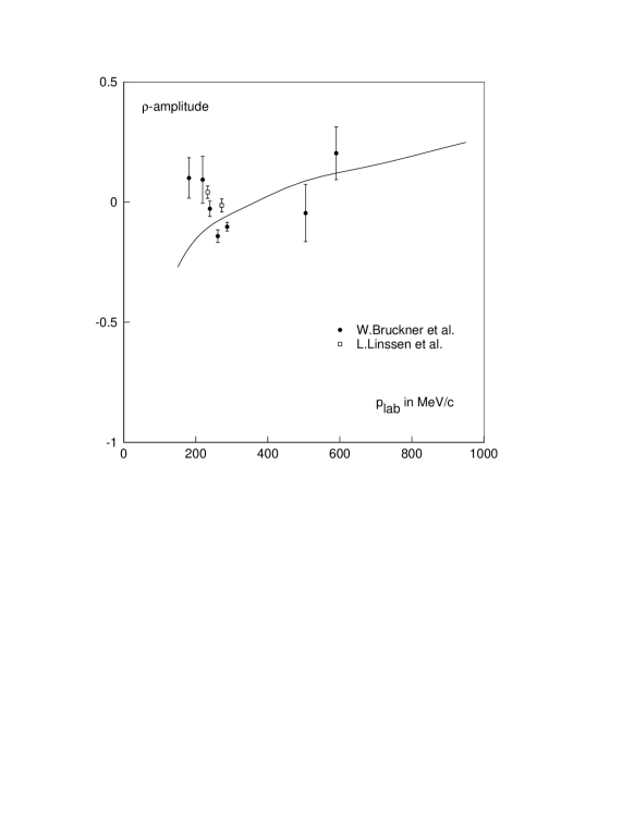
Figure 4: The $\rho$ amplitude. Data are from PS172 and PS173. The curve is the prediction from the Nijmegen PWA.

Another curious trend is the direct comparison between predictions of meson-exchange models and of simple quark-gluon models for the strangeness-exchange reaction. There are even serious proposals [54, 55] for experiments to distinguish between these models: it is proposed to measure the spin transfer in $\bar{p}p\rightarrow\bar{\Lambda}\Lambda$.

Let us make it clear from the outset, that we believe that all data must eventually be explained in terms of quark-gluon exchanges, because this is the underlying theory. However, for the analogous $N\!N$ interaction one has unfortunately not yet succeeded to give a proper explanation of the meson-exchange mechanism in terms of quarks and gluons exchanges. The theory is not so advanced yet. In the $\overline{N}\!N$ reactions we are of course in exactly the same situation. Using our PWA as a tool we determined the $\Lambda N\!K$ coupling constant and the mass of the exchanged kaon. This way we established beyond any doubt that the one-kaon-exchange potential is present in the transition potential and that again the tensor potential dominates. It is absolutely not necessary to measure the spin transfer to distinguish between the $K(494)$- and $K^{*}(892)$-exchange picture and a simple quark-gluon-exchange picture. This distinction has already been made using our PWA as a tool and using just the differential cross sections and polarizations.

It has become a fad to promote the measurements of spin-transfer and spin-correlation data, as if these data will solve all our troubles. For example in the already often mentioned Archamps Meeting Report [47] one can read that the longitudinal spin transfer is obviously a favorite of one of its authors. Somewhere else in the same report one finds the question: “Which new spin measurement would be crucial to confirm or rule out present models?” The answer to this last question is of course: None! When one measures differential cross sections, polarizations, spin transfers, or spin correlations, carefully enough, none of the present models will fit these new data, but adjustments will be made in the models in such a way that they do fit the data again. Physics is hard work from experimentalists as well as from theorists. One needs many and varied data and one single experiment has only a marginal influence.

Acknowledgments
Part of this work was included in the research program of the Stichting voor Fundamenteel Onderzoek der Materie (FOM) with financial support from the Nederlandse Organisatie voor Wetenschappelijk Onderzoek (NWO).

References

- [1] R.A. Kunne et al., Phys. Lett. B 206, 557 (1988); Nucl. Phys. B323, 1 (1989).
- [2] R. Bertini et al., Phys. Lett. B 228, 531 (1989); F. Perrot et al., ibid. 261, 188 (1991).
- [3] R.A. Kunne et al., Phys. Lett. B 261, 191 (1991).
- [4] R. Timmermans, Th.A. Rijken, and J.J. de Swart, Phys. Rev. Lett. 67, 1074 (1991).
- [5] R. Birsa et al., Phys. Lett. B 246, 267 (1990); ibid. 273, 533 (1991).
- [6] R. Birsa et al., Phys. Lett. B 302, 517 (1993).
- [7] P.D. Barnes et al., Phys. Lett. B 189, 249 (1987); ibid. 199, 147 (1987); 229, 432 (1989); Nucl. Phys. A526, 575 (1991).
- [8] P.D. Barnes et al., Phys. Lett. B 246, 273 (1990).
- [9] R. Timmermans, Th.A. Rijken, and J.J. de Swart, Phys. Lett. B 257, 227 (1991).
- [10] A. Pais and R. Jost, Phys. Rev. 87, 871 (1952); C. Goebel, Phys. Rev. 103, 258 (1956); T.D. Lee and C.N. Yang, Il Nuovo Cimento 3, 749 (1956).
- [11] M.S. Spergel, Il Nuovo Cimento 47A, 410 (1967).
- [12] O.D. Dal’karov and F. Myhrer, Il Nuovo Cimento 40A, 152 (1977).
- [13] A. Delville, P. Jasselette, and J. Vandermeulen, Am. J. Phys. 46, 907 (1978).
- [14] R.A. Bryan and R.J.N. Phillips, Nucl. Phys. B5, 201 (1968); ibid. B7, 481(E) (1968).
- [15] E. Eisenhandler et al., Nucl. Phys. B113, 1 (1976).
- [16] C.B. Dover and J.-M. Richard, Phys. Rev. C 21, 1466 (1980); ibid. 25, 1952 (1982).
- [17] M. Kohno and W. Weise, Nucl. Phys. A454, 429 (1986).
- [18] T. Hippchen, K. Holinde, and W. Plessas, Phys. Rev. C 39, 761 (1989).
- [19] J. Carbonell, O.D. Dal’karov, K.V. Protasov, and I.S. Shapiro, Nucl. Phys. A535, 651 (1991).
- [20] J. Côté, M. Lacombe, B. Loiseau, B. Moussallam, and R. Vinh Mau, Phys. Rev. Lett. 48, 1319 (1982).
- [21] M. Pignone, M. Lacombe, B. Loiseau, and R. Vinh Mau, Phys. Rev. Lett. 67, 2423 (1991).
- [22] M. Lacombe, B. Loiseau, J.-M. Richard, R. Vinh Mau, J. Côté, P. Pirès, and R. de Tourreil, Phys. Rev. C 21, 861 (1980).
- [23] P.H. Timmers, W.A. van der Sanden, and J.J. de Swart, Phys. Rev. D 29, 1928 (1984).
- [24] G.Q. Liu and F. Tabakin, Phys. Rev. C 41, 665 (1990).
- [25] O.D. Dal’karov, J. Carbonell, and K.V. Protasov, Sov. J. Nucl. Phys. 52, 1052 (1990), (Yad. Fiz. 52, 1670 (1990)).
- [26] R. Timmermans, Ph.D. thesis, University of Nijmegen (1991); R. Timmermans, Th. A. Rijken, and J.J. de Swart, in preparation.
- [27] J.R. Bergervoet, P.C. van Campen, W.A. van der Sanden, and J.J. de Swart, Phys. Rev. C 38, 15 (1988).
- [28] J.R. Bergervoet, P.C. van Campen, R.A.M. Klomp, J.-L. de Kok, T.A. Rijken, V.G.J. Stoks, and J.J. de Swart, Phys. Rev. C 41, 1435 (1990).
- [29] V.G.J. Stoks, R.A.M. Klomp, M.C.M. Rentmeester, and J.J. de Swart, Phys. Rev. C 48, 792 (1993).
- [30] R. Timmermans, Th.A. Rijken, and J.J. de Swart, submitted for publication.
- [31] M.M. Nagels, T.A. Rijken, and J.J. de Swart, Phys. Rev. D 17, 768 (1978).
- [32] J.J. de Swart and M.M. Nagels, Fortschr. Phys. 26, 215 (1978).
- [33] M. Alston-Garnjost et al., Phys. Rev. Lett. 43, 1901 (1979).
- [34] A.S. Clough et al., Phys. Lett. B 146, 299 (1984); D.V. Bugg et al., Phys. Lett. B 194, 563 (1987).
- [35] W. Brückner et al., Phys. Lett. B 197, 463 (1987); ibid. 199, 596(E) (1987); Zeit. Phys. A335, 217 (1990).
- [36] R. Timmermans, Th.A. Rijken, and J.J. de Swart, Nucl. Phys. A479, 383c (1988); Phys. Rev. D 45, 2288 (1992).
- [37] F. Tabakin and R.A. Eisenstein, Phys. Rev. C 31, 1857 (1985).
- [38] P.H. Timmers, Ph.D. thesis, University of Nijmegen (1985).
- [39] J.A. Niskanen, Helsinki preprint HU-TFT-85-28.
- [40] M. Kohno and W. Weise, Phys. Lett. B 179, 15 (1986); Phys. Lett. B 206, 584 (1988); Nucl. Phys. A479, 433c (1988).
- [41] S. Furui and A. Faessler, Nucl. Phys. A468, 669 (1987).
- [42] P. Kroll and W. Schweiger, Nucl. Phys. A474, 608 (1987).
- [43] M.A. Alberg, E.M. Henley, and L. Wilets, Phys. Rev. C 38, 1506 (1988); Z. Phys. A331, 207 (1988).
- [44] P. LaFrance, B. Loiseau, and R. Vinh Mau, Phys. Lett. B 214, 317 (1988); P. LaFrance and B. Loiseau, Nucl. Phys. A528, 557 (1991).
- [45] J. Haidenbauer, K. Holinde, and J. Speth, Nucl. Phys. A562, 317 (1993).
- [46] P.M.M. Maessen, Th.A. Rijken, and J.J. de Swart, Phys. Rev. C 40, 2226 (1989).
- [47] F. Bradamante, R. Hess, and J.-M. Richard, Few-Body Systems 14, 37 (1993).
- [48] V. Stoks, R. Timmermans, and J.J. de Swart, Phys. Rev. C 47, 512 (1993).
- [49] R.A. Arndt, Z. Li, L.D. Roper, and R.L. Workman, Phys. Rev. Lett. 65, 157 (1990).
- [50] W. Brückner et al., Phys. Lett. B 169, 302 (1986).
- [51] W. Brückner et al., Phys. Lett. B 158, 180 (1985).
- [52] W. Brückner et al., Phys. Lett. B 166, 113 (1986); Zeit. Phys. A335, 217 (1990).
- [53] L. Linssen et al., Nucl. Phys. A469, 726 (1987).
- [54] J. Haidenbauer, K. Holinde, V. Mull, and J. Speth, Phys. Lett. B 291, 223 (1992).
- [55] M.A. Alberg, E.M. Henley, L. Wilets, and P.D. Kunz, Seattle preprint DOE/ER/40427-31-N93.