Determination of $|V_{ts}|$ from $D\rightarrow K^{*}\ell\nu$ and $B\rightarrow K^{*}\gamma$ data
via heavy quark symmetry and perturbative QCD

Abstract

We use heavy quark effective theory (HQET) and perturbative QCD to study the heavy meson – light vector meson transitions involved in $D$ and $B$ decays. HQET is used to relate the measured $D\rightarrow K^{*}\ell\nu$ vector and axial-vector form factors at four-momentum transfer $q^{2}=0$ to the $B\rightarrow K^{*}\gamma$ tensor and axial-tensor form factors at $q^{2}=16.5$ $\mbox{GeV}^{2}$. Perturbative QCD is then used to find matching conditions for the $B$-meson form factors at $q^{2}=0$. A five parameter “vector dominance” type fit of the two HQET form factors, consisting of single pole, double pole, and subtraction terms, is used to match the data at $q^{2}=16.5$ $\mbox{GeV}^{2}$ to QCD at $q^{2}=0$. The values at $q^{2}=0$ are compared with recent data on the exclusive rate for $B\rightarrow K^{*}\gamma$ decay to extract a value for the Cabibbo-Kobayashi-Maskawa matrix element $\mbox{$|V_{ts}|$}\ =0.035$, with 28% experimental uncertainty, and 32% theoretical uncertainty from higher order QCD effects and violations of heavy quark symmetry.

PACS: 13.20.Fe, 13.20.Jf

I Introduction

Rare $B$ decays are a sensitive probe of flavor changing processes. In particular, the quark level process $b\rightarrow s\gamma$ occurs mainly via a “penguin” type diagram that is sensitive to the Cabibbo-Kobayashi-Maskawa matrix element $|V_{ts}|$. A proper analysis of the penguin requires a treatment of leading logarithmic strong interaction corrections[1]. At low energies, assuming only standard model physics, it corresponds to the effective Hamiltonian

$$H_{\gamma}=\eta\,m_{b}\,\bar{s}\,\sigma^{\mu\nu}(1+\gamma_{5})\,b\,F_{\mu\nu}+\ldots\ ,$$ (2)

$$\hbox{where \ \ }\eta={G_{F}\,e\over\sqrt{2}\,16\pi^{2}}\,V_{tb}\,V^{*}_{ts}\,F_{2}(m^{2}_{t}/m^{2}_{W})\ .$$ (3)

The parameter $F_{2}$ includes the leading logarithmic corrections and is mildly sensitive to the top quark mass. It ranges from $0.59$ for $m_{t}=120$ GeV to $0.68$ for $m_{t}=210$ GeV. We will use the value $F_{2}=0.63$, which corresponds to $m_{t}=150$ GeV.

Recently, experimental evidence for this penguin has been found by the CLEO collaboration via the exclusive decay $B\rightarrow K^{*}\gamma$[2]:

$${\rm B.R.}(\mbox{$B\rightarrow K^{*}\gamma$})=(4.5\pm 1.7)\times 10^{-5}\ .$$ (4)

This is related to the decay rate via $\Gamma={\rm B.R.}/\tau_{B}$, where we use the $B$ meson lifetime $\tau_{B}=(1.29\pm 0.05)$ ps[3]. The theoretical expression for the exclusive rate of is given by

$$\Gamma(\mbox{$B\rightarrow K^{*}\gamma$})={|\eta|^{2}m_{b}^{2}\,(A^{(b)}(0)+B^{(b)}(0))^{2}\over 4\pi m_{B}^{3}}(m_{B}^{2}-m_{K^{*}}^{2})^{3}\ ,$$ (5)

where $A^{(b)}(0)$ and $B^{(b)}(0)$ are tensor form factors[4] determined by the matrix element $\langle K^{*}|\bar{s}\,\sigma^{\mu\nu}(1+\gamma_{5})\,b|B\rangle$ at $q^{2}=0$ and defined explicitly in section two. In this paper, we will study the consistency of the standard model with this data, by extracting from it a value for $|V_{ts}|$. Throughout this paper we will take $V_{tb}=1$ in the context of the standard model with three generations[3], although it should be clear from eqn. (1b) that we are really calculating the combination $|V_{ts}^{*}V_{tb}|$.

Unitary of the Cabibbo-Kobayashi-Maskawa mixing with three generations of quarks places a severe constraint the mixing angle $|V_{ts}|$. Following the conventions of the particle data group[3], $|V_{ts}|\approx|V_{ud}||V_{cb}|=0.041\pm 0.007$. An additional quark generation or the presence of vectorlike down type quarks (which appear in $SO(10)$ unification) would invalidate this result. The penguin itself is quite sensitive to non-standard model physics, particularly to the exchange of charged Higgs bosons[1, 5, 6], which can easily suppress or enhance the parameter $F_{2}$ by a factor of two. In principle, this can be used to place constraints on supersymmetry breaking parameters[7].

Quark model calculations of the hadron matrix elements and the subsequent branching ratio vary by an order of magnitude[8], and are therefore unreliable as a test of the standard model result for $|V_{ts}|$. Instead, we shall apply heavy quark effective theory (HQET). This is a model independent framework that relates processes where a heavy quark of mass $m_{Q}\gg\Lambda_{QCD}$ exchanges momenta smaller than $m_{Q}$ with the light degrees of freedom inside the hadron. HQET makes manifest the symmetries of the QCD Lagrangian that occur in the infinite heavy quark limit: a flavor symmetry which relates the mass splittings and decay amplitudes of hadrons with different heavy quark content, and a spin symmetry which simplifies the mass spectrum and relates the decay amplitudes of hadrons with the same heavy quark content, but with different heavy quark spin. The spin symmetry is analogous to the proton spin symmetry in the hydrogen atom spectrum, which is broken only weakly by the hyperfine splittings. (For a review of HQET, see [9, 10] and references therein.) For example, all of the form factors relevant in the semileptonic decay of a $B$ to a $D$ or $D^{*}$ (charmed) meson can be given in terms of a single universal function, to leading order in an expansion in $\Lambda_{QCD}/m_{Q}$, where $m_{Q}$ corresponds to $b$ and $c$ quarks masses. This so called Isgur-Wise function depends only on the relative four velocities of the initial and final heavy quarks, and is absolutely normalized at zero recoil.

HQET also has implications in heavy hadron to light hadron (heavy – light) transitions. The process $B\rightarrow\pi\ell\nu$ ,i.e., the decay of a heavy pseudoscalar meson ($s^{\pi}=0^{-}$) to a light pseudoscalar meson, has recently been studied in this context[11]. For the case at hand, ($B\rightarrow K^{*}\gamma$), we will need to consider the decay of a heavy pseudo-scalar meson to a light vector meson ($s^{\pi}=1^{-}$). Therefore, in Section 2 we will use the tensor formalism[12] to establish the most general form of any transition amplitude between a heavy pseudoscalar meson and a light vector meson consistent with HQET. Again, the strange quark is not treated as heavy compared to the QCD scale $\Lambda_{QCD}$.

To extract $|V_{ts}|$ from the data, we need to determine the combination of tensor form factors $A^{(b)}(0)+B^{(b)}(0)$ which occur in the $B\rightarrow K^{*}\gamma$ decay rate, eqn. (5). Here we apply heavy quark symmetry to relate this combination to the form factors associated with $D\rightarrow K^{*}\ell\nu$ data,

$$\langle K^{*}(p^{\prime},\epsilon)|\bar{s}\,\gamma^{\mu}(1-\gamma_{5})\,c|D(p)\rangle= {2i\epsilon^{\mu\nu\alpha\beta}\over m_{K^{*}}m_{D}}\epsilon^{*}_{\nu}{p^{\prime}}_{\alpha}p_{\beta}V(q^{2})-(m_{D}+m_{K^{*}})\epsilon^{*\mu}A_{1}(q^{2})$$ (6)

$$+{A_{2}(q^{2})\over m_{D}+m_{K^{*}}} \epsilon^{*}\cdot p(p+{p^{\prime}})^{\mu}+{A_{3}(q^{2})\over m_{D}+m_{K^{*}}}\epsilon^{*}\cdot p(p-{p^{\prime}})^{\mu}\ ,\$$ (7)

where $q^{2}=(p-{p^{\prime}})^{2}$. The form factor $A_{3}$ leads to unmeasurable contributions proportional to the electron mass. For $A_{1}$, $A_{2}$, and $V$, we will use the averages over data from experiments E653[13] ($D\rightarrow K^{*}e\nu$) and E691[14] ($D\rightarrow K^{*}\mu\nu$) at Fermilab given in refs. [15, 16]:

$$V(0)=0.95\pm 0.20\ ,\ \ A_{1}(0)=0.48\pm 0.05\ ,\ \ A_{2}(0)=0.27\pm 0.11\ .$$ (8)

These are the values of the form factors given at zero invariant momentum transfer, $q^{2}=0$, for the $D\rightarrow K^{*}\ell\nu$ system, extrapolated with a simple pole ansatz for the form factors. (The results are relatively insensitive to the form of the ansatz, because the data is taken in the narrow region $q^{2}=0$ to $q^{2}\approx 1\ \mbox{GeV}^{2}$.)

Heavy quark symmetry will relate the two decay systems in in the following way: since to leading order the heavy quark form factors calculated from the effective theory are independent of the heavy quark mass, they are functions only of the $K^{*}$ mass and the dimensionless parameter

$$w={v\cdot p^{\prime}\over m_{K^{*}}}\ ,$$ (9)

where $v$ is the velocity of the heavy meson and $p^{\prime}$ is the momentum of the final state $K^{*}$ meson. On the other hand form factors are given as a function of

$$q^{2}=m_{Q}^{2}+m_{K^{*}}^{2}-2m_{Q}m_{K^{*}}w\ ,$$ (10)

where $m_{Q}$ is the mass of the heavy meson. This means that $q^{2}=0$ for the $B\rightarrow K^{*}\gamma$ decay corresponds to $w\equiv w_{B}\approx 3.04$, while for the $D\rightarrow K^{*}\ell\nu$ decay, $q^{2}=0$ corresponds to $w\equiv w_{D}\approx 1.29$. We will show in section 2 that the heavy quark flavor and spin symmetries relate the $D\rightarrow K^{*}\ell\nu$ data given by (8) to the tensor form factors of the $B\rightarrow K^{*}\gamma$ decay at $w=w_{D}$, which corresponds via eqn. (10) to $q^{2}\approx 16.5\ \mbox{GeV}^{2}$ for the $B$ decay system. We must then evolve the $B$ decay form factors down to $q^{2}=0$, or equivalently, from $w_{D}$ up to $w_{B}$.

To determine the interpolating functions that can be used to evolve the form factors from $w_{D}=1.29$ to $w=3.04$, which for $B\rightarrow K^{*}\gamma$ decay is the kinematical point corresponding to the emission of an on shell photon, we will use Perturbative QCD. This is the appropriate description of strong processes involving the exchange of hard gluons, and corresponds to heavy – light transitions with a large value of the kinematical variable $w$, that is, far away from the “zero recoil” point $w=1$. Therefore, in Section 3 we develop the Brodsky-Lepage formalism[17] of perturbative QCD to calculate the HQET heavy – light form factors for “large” $w$, to leading order in the heavy quark mass expansion, and to leading order in $\alpha_{s}.$ We argue that the method is reliable at $w=w_{B}$, (corresponding to $\alpha_{s}\approx 0.20$), and use this perturbative calculation to place “matching constraints” on the interpolating form factors. Furthermore, we use perturbation theory to determine the leading violations of HQET – the order $w\cdot m_{K^{*}}/m_{Q}$ corrections.

We will use the $D\rightarrow K^{*}\ell\nu$ data to constrain the interpolating form factors at $w_{D}$, and perturbative QCD to constrain them at $w_{B}$. As discussed in section 4, this will enable us to make a five parameter fit to the two relevant heavy-light form factors required for the determination of $|V_{ts}|$. The parametrization is in terms of single pole, double pole, and a single subtraction (constant piece), consistent with “vector dominance” ideas.

This is a better way of fitting to perturbative QCD than simply assuming a pole form for the vector and axial-vector form factors because we require the parametrization to match the heavy – light form factors in the perturbative regime. This is not the same as matching the perturbative result in the limit $w\rightarrow\infty$, with $m_{Q}$ fixed; in this limit, perturbative QCD counting rules[18] do indeed indicate single pole dominance, but this is due to the $w\cdot m_{K^{*}}/m_{Q}$ corrections from the point of view of the HQET. The HQET limit corresponds to taking $m_{Q}\rightarrow\infty$, with $w$ fixed, and this is the correct way of performing perturbation theory in our case, since the evolution of the form factors occurs for $w\cdot m_{K^{*}}/m_{B}<1$. In fact, as we shall show in section 2, assuming a simple pole form for these form factors, with no subtactions, is inconsistent with heavy quark symmetry to leading order in heavy quark mass.

As a self consistency check, we use the absolute normalization of the $B$ decay form factors, obtained by HQET matching to the $D$ decay data, to estimate of the B-decay constant $f_{B}$ to leading order in QCD perturbation theory. This check, and further error estimates, are contained in section 5.

Section 6 is devoted to a discussion on how to systematically improve these results, and our conclusions.

II Heavy – light form factors

We shall first apply the tensor method[12] to the case of a heavy pseudoscalar meson $M_{Q}(v)$ decaying into the light vector meson $K^{*}(\epsilon,{p^{\prime}})$. This method is usually applied to the derivation of heavy to heavy meson form factors[9, 10], and recently has been used for the case of the heavy meson to light meson transition $B\rightarrow\pi\ell\nu$[11]. We will determine the most general form of heavy psuedoscalar to light vector form factors consistent with Lorentz invariance and heavy quark spin symmetry.

It is useful to consider the matrix element of the general operator $\bar{s}\Gamma Q$, where $\Gamma$ is an arbitrary product of gamma matrices, and $Q$ is a heavy quark Dirac field. To leading order in the HQET, $Q$ is replaced by its projection onto the quark (versus antiquark) field via the replacement $Q\rightarrow h^{(Q)}_{v}$, where $h^{(Q)}_{v}(x)=\exp{(im_{Q}v\cdot x)}{1+{v\!\!\!/}\over 2}Q(x)$, and $v$ is the heavy meson velocity obeying $v^{2}=1$. The relevant matrix element takes the form

$$\langle K^{*}(p^{\prime},\epsilon)|\bar{s}\,\Gamma\,h^{(Q)}_{v}|M_{Q}(v)\rangle=\sqrt{m_{K^{*}}m_{Q}}\,{\rm Tr}\left\{\Theta(v,{p^{\prime}},\epsilon^{*})\,\Gamma\,{1+{v\!\!\!/}\over 2}\gamma_{5}\right\}\ ,$$ (11)

where $p^{\prime}_{\mu}=m_{K^{*}}{v^{\prime}}_{\mu}$ is the $K^{*}$ momentum, and $\epsilon$ is the $K^{*}$ polarization vector which satisfies $\epsilon^{*}\cdot{p^{\prime}}=0$. The ${1+{v\!\!\!/}\over 2}$ in Eq. (11) explicitly projects the matrix element onto the heavy quark components of the heavy quark spinor, since in the infinite quark mass limit heavy antiquarks are not produced, and the $\gamma_{5}$ describes the pseudoscalar nature of the heavy meson. A simple way to understand eqn. (11) is by parametrizing the initial heavy meson as $|h^{(Q)}_{v}\gamma_{5}\ell\rangle$, where $\ell$ describes all of the light degrees of freedom in the heavy meson, and using the heavy quark propagator[9] $\langle h^{(Q)}_{v}{\bar{h}}^{(Q)}_{v}\rangle=(1+{v\!\!\!/})/2$ . The matrix function $\Theta$ encapsulates all of our ignorance of the dynamics of the light degrees of freedom of the heavy meson and the $K^{*}$ meson. It is explicitly independent of the heavy quark mass to leading order in HQET. The $\sqrt{m_{Q}}$ in eqn. (11) comes from the usual normalization of the heavy meson with respect to its energy.

More specifically, the scalar matrix $\Theta$ must be proportional to the polarization of the $K^{*}$ meson: $\Theta={\cal M}_{1}{\epsilon\!\!/}^{*}+{\cal M}_{2}v\cdot\epsilon^{*}$, where the ${\cal M}_{i}$ are matrix functions of $m_{K^{*}}$ and $w$ defined in eqn. (9). Furthermore, using the fact that ${1+{v\!\!\!/}\over 2}{v\!\!\!/}={1+{v\!\!\!/}\over 2}$, the only possible matrix structure of each ${\cal M}_{i}$ within the trace is $\theta+{v\!\!\!/}^{\prime}\theta^{\prime}$, where the $\theta$ and $\theta^{\prime}$ are real functions of $v\cdot{p^{\prime}}$. Therefore, one can parametrize $\Theta$ in terms of only four linearly independent form factors, $\theta_{i}(m_{K^{*}},w)$,

$$\Theta=(\theta_{1}+{v\!\!\!/}^{\prime}\theta_{2}){\epsilon\!\!/}^{*}+(\theta_{3}+{v\!\!\!/}^{\prime}\theta_{4})v\cdot\epsilon^{*}\ .$$ (12)

We will refer to Eqs. (11,12) as the heavy – light matrix elements for the decay of a heavy pseudoscalar into a light vector. This is the relativistic generalization (where the heavy quark is not necessarily in its rest frame) of the heavy – light matrix elements obtained in Ref.[19]

Since the $b$ and $c$ quarks are not infinitely heavy, the relation between operators in QCD and in the heavy quark effective theory is non-trivial. In the leading logarithmic approximation, the relation between the QCD currents and heavy quark effective theory currents discussed above is $\bar{s}\Gamma Q=C_{Q}(\mu)\bar{s}\Gamma h_{v}^{(Q)}$, where the coefficient functions are[20] $C_{Q}(\mu)=\left[\alpha(m_{Q})/\alpha(\mu)\right]^{-6/(33-2N)}$, $N$ denotes the number of flavors below the $m_{Q}$ scale, and $\mu$ is the infrared subtraction point. It is useful to define $\theta^{(Q)}_{i}=C_{Q}\theta_{i}$. The $\theta^{(Q)}_{i}$ are subtraction point independent and satisfy

$$\theta^{(b)}_{i}=C_{cb}\,\theta^{(c)}_{i}\ ,\ \ C_{cb}=\left[{\alpha(m_{b})\over\alpha(m_{c})}\right]^{-6/25}\ .$$ (13)

We use $\alpha_{s}(m_{b})/\alpha_{s}(m_{c})=[\ln{(m_{D}^{2}/\Lambda_{QCD})}/\ln{(m_{B}^{2}/\Lambda_{QCD})}]$, which for $\Lambda_{QCD}=300$ MeV gives $C_{cb}=1.114$.

Eqs. (11, 12) place strong constraints between the form factors corresponding to different matrix elements. For $\Gamma=\sigma^{\mu\nu}$, the matrix element is given by

$$\langle K^{*}(p^{\prime},\epsilon)|\bar{s}\,\sigma^{\mu\nu}\,Q|M_{Q}(p)\rangle=\epsilon^{\mu\nu\alpha\beta}\left(A^{(Q)}\epsilon^{*}_{\alpha}p_{\beta}+B^{(Q)}\epsilon^{*}_{\alpha}{p^{\prime}}_{\beta}+C^{(Q)}\epsilon^{*}\cdot p\,p_{\alpha}{p^{\prime}}_{\beta}\right)\ .$$ (14)

Using the identity $\sigma^{\mu\nu}\gamma_{5}=-{1\over 2}i\epsilon^{\mu\nu\alpha\beta}\sigma_{\alpha\beta}$ one can immediately write the form factors for the $\Gamma=\sigma^{\mu\nu}\gamma_{5}$ matrix element,

$$\langle K^{*}(p^{\prime},\epsilon)|\bar{s}\,\sigma^{\mu\nu}\gamma_{5}\,Q|M_{Q}(p)\rangle=i\bigg{[} A(\epsilon^{*\mu}p^{\nu}-\epsilon^{*\nu}p^{\mu})+B(\epsilon^{*\mu}{p^{\prime}}^{\nu}-\epsilon^{*\nu}{p^{\prime}}^{\mu})$$ (16)

$$\mbox{}+C\epsilon^{*}\cdot p\,(p^{\mu}{p^{\prime}}^{\nu}-p^{\nu}{p^{\prime}}^{\mu})\bigg{]}\ .$$

Evaluating these matrix elements using Eqs. (11,12) gives relations between the “tensor” form factors $A,B,C$, and the heavy – light form factors $\theta_{i}$,

$$A^{(Q)}=-2\sqrt{m_{K^{*}}\over m_{Q}}\theta^{(Q)}_{1}\ ,\ \ B^{(Q)}=2\sqrt{m_{Q}\over m_{K^{*}}}\theta^{(Q)}_{2}\ ,\ \ C^{(Q)}={2\,\theta^{(Q)}_{4}\over m_{Q}^{3/2}m_{K^{*}}^{1/2}}\ .$$ (17)

The vector and axial-vector matrix elements can be parametrized as

$$\langle K^{*}(p^{\prime},\epsilon)|\bar{s}\,\gamma^{\mu}\,Q|M_{Q}(p)\rangle=iD^{(Q)}\epsilon^{\mu\nu\alpha\beta}p_{\nu}\epsilon^{*}_{\alpha}{p^{\prime}}_{\beta}\ ,$$ (19)

$$\langle K^{*}(p^{\prime},\epsilon)|\bar{s}\,\gamma^{\mu}\gamma_{5}\,Q|M_{Q}(p)\rangle=E^{(Q)}\epsilon^{*\mu}+F^{(Q)}\epsilon^{*}\cdot pp^{\mu}+G^{(Q)}\epsilon^{*}\cdot p{p^{\prime}}^{\mu}\ .$$ (20)

Evaluating these matrix elements using the heavy – light parameterization yields

$$D^{(Q)}={-2\,\theta^{(Q)}_{2}\over\sqrt{m_{K^{*}}m_{Q}}}\ ,\ \ E^{(Q)}=2\sqrt{m_{K^{*}}m_{Q}}\theta^{(Q)}_{1}-{2\,p\cdot{p^{\prime}}\over\sqrt{m_{K^{*}}m_{Q}}}\theta^{(Q)}_{2}\ ,$$ (22)

$$F^{(Q)}=-2\sqrt{m_{K^{*}}m_{Q}}{\theta^{(Q)}_{3}\over m_{Q}^{2}}\ ,\ \ G^{(Q)}={2(\theta^{(Q)}_{2}+\theta^{(Q)}_{4})\over\sqrt{m_{K^{*}}m_{Q}}}\ .$$ (23)

Since the seven form factors for the matrix elements are given in terms of only four heavy – light form factors, there are three relations relations between them for each heavy meson $M_{Q}$:

$$A={-E+(p\cdot{p^{\prime}})D\over m_{Q}}\ ,\ \ B=-m_{Q}D\ ,\ \ C={G+D\over m_{Q}}\ .$$ (24)

These relations explicitly relate the tensor form factors to the vector and axial-vector form factors for a given heavy meson $M_{Q}$ transition to $K^{*}$. They represent the explicit realization of the heavy quark spin symmetry for the heavy pseudoscalar meson decay to a light vector. Equivalent relations, determined via analysis in the heavy quark rest frame, are found in refs. [4, 19]. This confirms our analysis which led to eqns. (11,12).

The relationships between the heavy – light form factors at the kinematical point $w_{D}=(m_{D}^{2}+m_{K^{*}}^{2})/2m_{D}m_{K^{*}}\approx 1.29$ and the experimentally measured $D\rightarrow K^{*}\ell\nu$ form factors are

$$\theta^{(c)}_{1}(w_{D}) ={m_{D}+m_{K^{*}}\over 2\sqrt{m_{D}m_{K^{*}}}}\left[A_{1}(0)-{m_{K^{*}}^{2}+m_{D}^{2}\over(m_{D}+m_{K^{*}})^{2}}V(0)\right]\ ,$$ (26)

$$\theta^{(c)}_{2}(w_{D}) =-{\sqrt{m_{K^{*}}m_{D}}\over m_{K^{*}}+m_{D}}V(0)\ ,$$ (27)

$$\theta^{(c)}_{3}(w_{D}) -{m_{D}\over m_{K^{*}}}\theta^{(c)}_{4}(w_{D})=\sqrt{m_{D}\over m_{K^{*}}}{m_{D}\over m_{D}+m_{K^{*}}}[A_{2}(0)-V(0)]\ ,$$ (28)

$$\theta^{(c)}_{3}(w_{D}) +{m_{D}\over m_{K^{*}}}\theta^{(c)}_{4}(w_{D})=\sqrt{m_{D}\over m_{K^{*}}}{m_{D}\over m_{D}+m_{K^{*}}}[A_{3}(0)+V(0)]\ .$$ (29)

From the data, the values of $\theta_{1}$, $\theta_{2}$ and the combination $\theta_{3}-(m_{D}/m_{K^{*}})\theta_{4}$ at $w_{D}$ can be extracted,

$$\theta^{(c)}_{1}(w_{D})=-(0.06\pm 0.13)\ ,\ \ \theta^{(c)}_{2}(w_{D})=-(0.44\pm 0.09)\ ,$$ (31)

$$\theta^{(c)}_{3}(w_{D})-{m_{D}\over m_{K^{*}}}\theta^{(c)}_{4}(w_{D})=-(0.66\pm 0.22)\ ,$$ (32)

where we have quoted experimental uncertainty.

Treatment of the strange quark as heavy in the context of HQET has been considered in the literature[21]. Eqns. (II) indicate that $\Lambda_{QCD}/m_{s}$ corrections are large. In an expansion in terms of the strange quark mass, the trace formula eqn. (11) for the heavy – light form factor is modified by addition of ${\epsilon\!\!/}^{*}(1+{v\!\!\!/}^{\prime})/2$, to project onto the “heavy” strange quark (verses antiquark). This exercise gives in the standard result for the Isgur-Wise function $\xi$. Using the heavy – light parametrization, one finds that $\xi=\theta_{1}-\theta_{2}$, and further that $\theta_{1}+\theta_{2}$, $\theta_{3}$, and $\theta_{4}$ each vanish to leading order in the $1/m_{s}$ expansion. Clearly, the vanishing relations are strongly violated by the data given above.

Heavy quark flavor symmetry relates the heavy – light form factors for $D$ decay to those for $B$ decay, as given in equation (13). The data determines $\theta_{1}$ and $\theta_{2}$, which in turn give the tensor form factors required for the extraction of $|V_{ts}|$ via eqn. (17). We are then left to determine the running of the form factors from $w_{D}$ to $w_{B}$. This is a dynamical question, and the kinematical heavy quark symmetry cannot give us the answer.

There are two “straightforward” avenues of approach to this problem, QCD sum rules[22], and perturbative QCD[17]. In the next section, we will discuss the later approach. We note that in the literature, a third approach is discussed, which is to make an outright guess as to the $q^{2}$ dependence of the form factors, following vector dominance ideas. To see the danger in this, consider assuming the standard single pole vector dominance ansatz for the vector and axial vector form factors $V(q)$ and $A_{1}(q)$ for the $B$ meson decay. This means that $V$ and $A_{1}$ are of the form $m^{2}_{T}/(q^{2}-m^{2}_{T})$, where $m_{T}$ a vector or axial vector threshold mass above the $B$ meson mass. Via eqns. (9,10), in terms of the more relevant HQET variable $w$, single pole dominance is of the form $1/w$, plus order $\Lambda_{QCD}/m_{Q}$ corrections. However, now that we have correctly parametrized the heavy – light form factors, it becomes clear that this form is incompatible with leading order HQET. Since $V\propto\theta_{2}$, and $A_{1}\propto(\theta_{1}-w\theta_{2})$, $A_{1}$ must have a “large” subtraction if the vector form factor obeys single pole dominance.

III $B\rightarrow K^{*}\gamma$ form factors at large $w$ from perturbative QCD

In the previous section we have used HQET to relate the form factors in $D\rightarrow K^{*}e\nu$ with those in $B\rightarrow K^{*}\gamma$ at $w_{D}=1.29$. However the physical value of $w$ for $B\rightarrow K^{*}\gamma$ that corresponds to an on shell photon is $w_{B}=3.05$. This value for the $B$ decay is in the regime of large $w$ far from zero recoil. How does one estimate the behavior of the form factors in this regime? First consider the treatment of heavy meson to heavy meson transitions by heavy quark symmetry. All form factors are determined from the Isgur-Wise function $\xi(w)$ and heavy quark symmetry fixes the value $\xi(w)=1$. For large enough values of $w$ the Brodsky-Lepage method of determining form factors from perturbative QCD can be invoked. To leading order, the Brodsky- Lepage formalism essentially includes the exchange of a single hard gluon between the initial or final heavy quark and its spectator quark. Assumptions about the meson wave functions, motivated by QCD sum rules and experiment[22] are made to fix the soft behavior of the amplitude. This method determines[23] the behavior of the Isgur-Wise function at large $w$. For $m_{Q}/\Lambda_{QCD}>w\gg 1$, $\xi(w)\sim{\alpha_{s}(m_{Q})\over{w^{2}}}$. As discussed in the previous section, this corresponds to a dipole in the sense of a vector dominance model. For the true asymptotic regime of $w>m_{Q}/\Lambda_{QCD}$, $\zeta(w)\sim{\alpha_{s}(Q)\over{w}}$, where $Q^{2}=-q^{2}$. This is in accordance with QCD dimensional-counting rules[18].

We shall essentially follow the same procedure in discussing heavy meson to light meson transitions. In this case of course we have $\theta_{1},\theta_{2},\theta_{3}$ and $\theta_{4}$ instead of the single Isgur-Wise function. Although we don’t have the convenient normalization at $w=1$, we can use instead the $D\rightarrow K^{*}e\nu$ data to determine the thetas at $w=1.29$. The fact that the kinetic point corresponding to $B\rightarrow K^{*}\gamma$ at $w=3.05$ is far from zero recoil is a virtue; it is in just the right regime for both perturbative QCD and heavy quark symmetry to be valid. That is, if $w$ is close to $1$, perturbative QCD is not valid, while if $w>m_{Q}/\Lambda_{QCD}$, then $w\cdot\Lambda_{QCD}/m_{Q}$ corrections dominate the HQET.

We now briefly describe standard aspects of the Brodsky-Lepage formalism as it applies to the case at hand. The soft nonperturbative part of the physics is encapsulated in quark distribution amplitudes $\phi(x,P,Q)$, for each meson, which denote the fraction $0<x<1$ of momentum $P$ carried by the valence quark of the meson. To leading order in the calculation, the antiquark carries momentum $(1-x)$; it can be argued that gluon and non-valence quark corrections are small for large momentum exchange via the QCD dimensional-counting rules. The parameter $Q$ denotes the subtraction point at which the distribution amplitudes are evaluated. Given a distribution amplitude $\phi$ at $Q_{0}$, $\phi(Q)$, for $Q>Q_{0}$ can be determined[17]. The dependence is logarithmic in $Q$, and $\phi$ asymptotically approaches $\phi\propto x(1-x)$. We shall initially consider two distribution amplitudes for the $K^{*}$ meson, as shown in fig. 1,

FIG. 1.: Two choices for the $K^{*}$ distribution amplitude. The solid curve is $\bar{\phi}_{1}(x)$, and the dashed curve is $\bar{\phi}_{czz}(x)$, as defined in the text. Both are normalized to unit area.

$$\bar{\phi}_{1}=6x(1-x)\ .$$ (34)

$$\bar{\phi}_{czz}=-12x^{2}(1-x)^{2}+{42\over 5}x(1-x)\ .$$ (35)

The second of these is the Chernyak-Zhitnitsky-Zhitnitsky[24] distribution amplitude for the $K^{*}$ at $Q^{2}=1.5\ \mbox{GeV}^{2}$. The integrals over $x$ for the functions are both normalized. However, the correct normalization is given by $\phi=f_{K^{*}}\bar{\phi}/2\sqrt{6}$, where $f_{K^{*}}$ is the meson decay constant (With this normalization, the pion decay constant $f_{\pi}=131$ MeV[3]).

For the momentum fraction of the heavy $b$ quark inside the initial $B$, we use the peaking approximation. The distribution amplitude for heavy quarks must have a large maximum near the end point $x=1-{\bar{\Lambda}/m_{Q}}$, and width $\bar{\Lambda}/m_{Q}$, where $m_{Q}=m_{q}+\bar{\Lambda}$. We use[10] $\bar{\Lambda}=0.5\ \mbox{GeV}$ as the typical amount of mass in the heavy meson due to the light degrees of freedom and make the approximation

$$\phi_{Q}(x)={1\over 2\sqrt{6}}f_{Q}\delta(1-x-{\bar{\Lambda}\over m_{Q}})\ .$$ (36)

The error induced by this approximation is of order $\bar{\Lambda}/m_{Q}$, which we are systematically neglecting in this paper.

The initial and final states are given by convoluting the distribution amplitudes with on-shell spinors of the quark and antiquark,

$$\Psi=\phi\sum_{\lambda,\lambda^{\prime}}f_{\lambda\lambda^{\prime}}\,u_{\lambda}(xP)\,\bar{v}_{\lambda^{\prime}}((1-x)P)\ ,$$ (37)

where $\lambda$ and $\lambda^{\prime}$ denote sums over helicities. In the context of the peaking approximation, $({P\!\!\!/}-m_{Q})u_{\lambda}(xP)=0$, and $({P\!\!\!/}+m_{Q})v_{\lambda^{\prime}}=0$. By applying these equations to the helicity sums, we find

$$\Psi_{Q}={\phi_{Q}(x)\over\sqrt{2}}(m_{Q}+{P\!\!\!/})\gamma_{5}\ .$$ (38)

For the $K^{*}$, we replace the $\gamma_{5}$ with ${\epsilon\!\!/}$, and let $m_{Q}\rightarrow m_{S}$. The last substitution is strictly not rigorous, because we are not using a peaking approximation for the $K^{*}$ distribution amplitude. This will induce errors of order $m_{K^{*}}/M_{B}$ in the final results. Required for the calculation is the conjugate of the state, $\bar{\Psi}_{K^{*}}=\gamma^{0}\Psi_{K^{*}}^{\dagger}\gamma^{0}$,

$$\bar{\Psi}_{K^{*}}=-{\phi_{K^{*}}(x)\over\sqrt{2}}{\epsilon\!\!/}^{*}(m_{K^{*}}+{P\!\!\!/})\ .$$ (39)

Our calculation will include the exchange of a single hard gluon between the initial heavy or $s$ quark and its spectator quark. The two diagrams are shown in figure 2(a,b), representing respectively the single gluon exchange between the heavy or $s$ quark and its spectator. Here $\Gamma$ represents the operator responsible for the heavy to light transition, as in the previous section.

FIG. 2.: The two Born amplitudes contributing to $M_{Q}\rightarrow K^{*}$ decay. The symbol $\Gamma$ denotes an arbitrary Dirac matrix associated with the decay.

These diagrams yield the contribution to the hard scattering amplitude $T_{\Gamma}$ from perturbative QCD. We use the identity $T^{a}T^{a}={4\over 3}I_{c}$ where $I_{c}$ is the 3x3 identity matrix of color space. The Brodsky-Lepage formalism tells us that the full amplitude at large $w$ is given by

$$<K^{*}|\bar{s}\Gamma Q|M_{Q}>=\int dxdy\mbox{{\rm Tr}}\bar{\Psi}_{K^{*}}(y)T_{\Gamma}(y,x)\Psi_{Q}(x){\hbox{}}$$ (40)

Both diagrams are infared (IR) divergent when the momentum flowing through the gluon line vanishes. Fig. (2b) also has an IR divergence associated with the strange quark going on-shell for small but finite gluon momentum transfer. These IR divergences are fictitious[17] and irrelevant at large recoil. The region of $y$ integration associated with the IR problem corresponds to the Drell-Yan-West[25] end point region, which is assumed to be cut off by a Sudakov form factor. Physically, the mutually canceling effects of multi-gluon exchange cut off this region, due to the fact that the color singlet meson decouples from soft gluons in the IR limit.

Following the cited literature, we apply a transverse momentum cutoff to suppress IR effects. In the rest frame of the heavy quark, we have the following picture. The momentum of the $K^{*}$ is given by $m_{K^{*}}(\cosh\theta,0,0,\sinh\theta)$. In this frame, the variable $w=\cosh\theta$, and the spacelike gluon momentum is $k_{3}=(1-y)m_{K^{*}}\sinh\theta$. This is the transverse momentum of the gluon, associated with transverse momentum of $p-p^{\prime}$. Large transverse momentum means that this is larger than the typical momentum associated with the light degrees of freedom, $\bar{\Lambda}$. Therefore we apply the cutoff

$$1-y>{\bar{\Lambda}\over m_{K^{*}}\sqrt{w^{2}-1}}.$$ (41)

The calculation is done in Feynman gauge. To extract the heavy – light form factors, an expansion of the perturbative expression in powers of $1/m_{Q}$ must be done. The leading terms for the gluon, strange quark, and heavy quark denominators ($k^{2}-m^{2}$ in each case), in the peaking approximation, are given by

$$D_{g} = (1-y)^{2}m_{K^{*}}^{2}+\bar{\Lambda}^{2}-2\bar{\Lambda}m_{K^{*}}(1-y)w\ ,$$ (43)

$$D_{s} = m_{K^{*}}^{2}-m_{s}^{2}+\bar{\Lambda}^{2}-2\bar{\Lambda}m_{K^{*}}w\equiv m_{K^{*}}\Delta_{s}\ ,$$ (44)

$$D_{Q} = 2m_{Q}(\bar{\Lambda}-(1-y)m_{K^{*}}w)\equiv m_{Q}\Delta_{Q}$$ (45)

By comparing the perturbative expression to the heavy – light parametrization (11), we find

$$\theta_{1} = \kappa(I_{Q}-{{\bar{\Lambda}-m_{s}}\over m_{K^{*}}}I_{S})\ ,$$ (47)

$$\theta_{2} = -\kappa(I_{Q}+I_{S})\ ,$$ (48)

$$\theta_{3} = -\kappa{2\bar{\Lambda}\over m_{K^{*}}}I_{s}\ ,$$ (49)

$$\theta_{4} = 0\ ,$$ (50)

to leading order in the $1/m_{Q}$ expansion. The constant $\kappa$ is

$$\kappa=f_{K^{*}}f_{Q}{\sqrt{m_{K^{*}}m_{Q}}\over m_{K^{*}}^{3}}{4\pi\alpha_{s}\over 9}\ .$$ (51)

From general heavy quark symmetry arguments[10] and the perturbative calculation done here, one finds that $f_{Q}\sim 1/\sqrt{m_{Q}}$ for large mass $m_{Q}$, and therefore $\kappa$ is finite and non-vanishing in the infinite heavy quark limit. The scale of $\alpha_{s}$ is set by the $M_{Q}$ meson mass. We will use for the $B$ meson $\alpha_{s}=0.20$. The functions $I_{Q}$ and $I_{s}$ denote the integrals over the momentum fraction $y$ from figure (2a) and (2b) respectively,

$$I_{Q} = \int_{0}^{1-\epsilon}dy\bar{\phi}^{\dagger}_{K^{*}}(y){m_{K^{*}}^{3}\over\Delta_{Q}D_{g}}\ ,$$ (53)

$$I_{s} = \int_{0}^{1-\epsilon}dy\bar{\phi}^{\dagger}_{K^{*}}(y){m_{K^{*}}^{3}\over\Delta_{s}D_{g}}\ ,$$ (54)

where $\epsilon$ denotes the IR cutoff given by eqn. (41). We provide the exact integrals for arbitrary wave function and cutoff in appendix A. For the distribution amplitudes $\phi_{1}$ and $\phi_{czz}$ defined above, they are plotted in fig. 3.

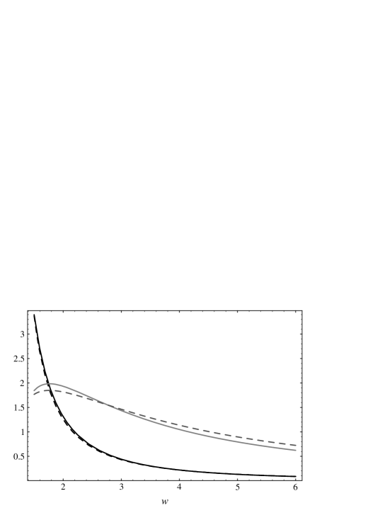
FIG. 3.: The two integrals $F_{S}$ (black curve) and $F_{Q}$ (gray curve) as defined in the text. The solid (dashed) curves are for the $\phi_{1}$ ($\phi_{czz}$) $K^{*}$ distribution amplitude.

From these figures, one can observe that the Drell-Yan-West region is turning over $I_{Q}$ at $w\sim 2$; that is, the loss of integral due to the IR cutoff is “beating” the IR divergence around this region. The integral $I_{Q}$ turns over at a smaller value of $w$ because of the additional strange quark pole. For the remainder of this paper, we will study only the $\phi_{1}$ case.

To study the region (in $w$) of validity of this calculation, one can compare the asymptotic expansion, in powers of $1/w$, to the full result for $\theta_{1}$ and $\theta_{2}$. To leading orders in this expansion,

$$\theta_{1}(w) \sim {\ln w\over w^{2}}\ ,$$ (56)

$$\theta_{2}(w) \sim {\ln w\over w^{2}}-{0.23\over w^{2}}\ .$$ (57)

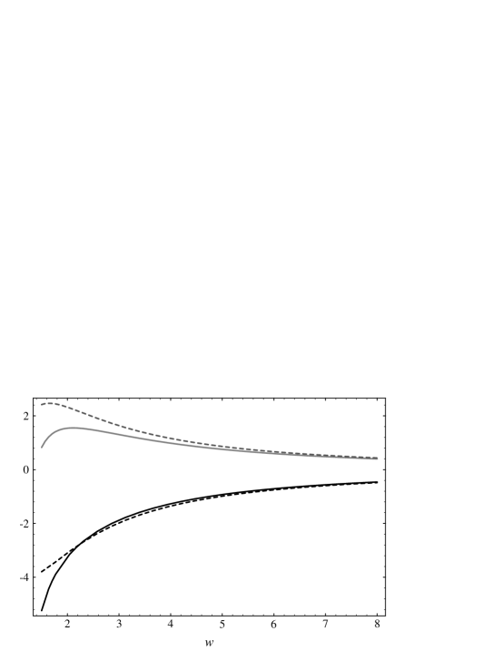
FIG. 4.: The un-normalized heavy-light form factors $\theta_{1}/\kappa$ (gray) and $\theta_{2}/\kappa$ (black), with their asymptotic behavior (dashed).

We note that $\theta_{1}$ also possesses a ${1/w^{2}}$ term but in our case it is numerically small. In fig. 4, the full and asymptotic (to order $1/w^{2}$) values of $\theta_{1}/\kappa$ and $\theta_{2}/\kappa$ are plotted, for the $\phi_{1}$ distribution amplitude. For $w<2$, less than two thirds of the integration region over $y$ is included by the Drell-Yan-West cutoff, indicating a large soft cutoff dependence to the amplitude. Our perturbative QCD result does not give a reliable estimate of the form factor in this regime. For $w=3$, the Drell-Yan-West region cuts off about $18\%$ of the momentum fraction integral, and the match between the full and asymptotic functions is reasonable, as shown in fig. 4. For $w>6$ the next to leading order $w\ m_{K^{*}}/m_{Q}$ corrections begin to dominate, and the leading order $\theta_{i}$ do not meaningfully describe the amplitude. We will discuss the effect of the next to leading order corrections in sec. 5.

Note that the parametric form of the thetas given by eqn. (III) has the correct heavy – heavy limit. As $m_{s}$ is taken to infinity, the integrals $I_{Q}$ and $I_{s}$ remain finite and non-vanishing, and $\xi=\theta_{1}-\theta_{2}$ is the leading contribution.

IV Interpolating functions and determination of $|V_{ts}|$

For $w$ less than or equal to about 2, interpolating functions for the heavy – light form factors are definitely required. Our strategy is to obtain such an interpolating function that is consistent with the data for $D\rightarrow K^{*}e\nu$ at $w=1.29$, matches the QCD calculation at $w=3.05$, and is consistent with vector dominance ideas. For the calculation of $V_{ts}$, we need to find interpolating functions for $\theta_{1}$ and $\theta_{2}$. As input to determine their forms, we use the two data points at $w=w_{D}$, and the three ratios

$$r_{1}={\theta_{1}^{\prime}(w_{B})\over\theta_{1}(w_{B})},\ \ r_{2}={\theta_{2}^{\prime}(w_{B})\over\theta_{2}(w_{B})},\ \ r_{3}={\theta_{1}(w_{B})\over\theta_{2}(w_{B})}\ .$$ (58)

These three ratios are determined by perturbative QCD in the context of the Brodsky - Lapage formalism. For the $\phi_{1}$ distribution amplitude, $r_{1}=0.2776$, $r_{2}=0.4403$, and $r_{3}=-0.6991$. These values can be systematically improved by higher order (in $\alpha_{s}$) calculations[29]. As discussed in the next section, we have reason to believe that the $\alpha_{s}$ contribution is a good approximation to the full result. We will consider a five parameter fit to the two form factors. Vector dominance ideas, that the amplitude is dominated by intermediate $b\bar{s}$ resonances, dictate that reasonable forms for the interpolating form factors are $1/w$ (single pole), $1/w^{2}$ (dipole), or a constant (subtraction). A subtraction is not considered for $\theta_{2}$ because the physical axial-vector form factor $E\sim(\theta_{1}-w\theta_{2})$, so that a constant term in $\theta_{2}$ would correspond to $E\sim w+\ldots$ which is “inconsistent” with vector dominance.

The interpolating functions used are

$$\theta_{1} = a\left({c\over w^{2}}+{d\over w}\right)+b\ ,$$ (60)

$$\theta_{2} = a\left({e\over w^{2}}+{f\over w}\right)\ .$$ (61)

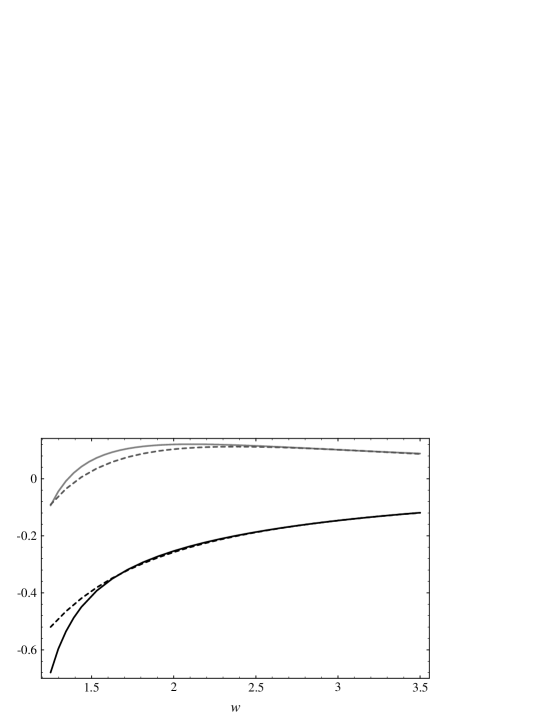
FIG. 5.: The normalized heavy-light form factors $\theta_{1}$ (gray) and $\theta_{2}$ (black), with their parametrizations with respect to the $K^{*}$ data (dashed).

The theoretical constraints, that the slopes of $\theta_{1},\theta_{2}$ and the ration $\theta_{1}/\theta_{2}$ at $w_{B}$ match the perturbative result give

$$c = -(r_{3}-b/a)w_{B}^{2}+r_{1}r_{3}w_{B}^{3}\ ,$$ (63)

$$d = 2w_{B}(r_{3}-b/a)-r_{1}r_{3}w_{B}^{2}\ ,$$ (64)

$$e = -w_{B}^{2}+r_{2}w_{B}^{3}\ ,$$ (65)

$$f = 2w_{B}-r_{2}w_{B}^{2}\ ,$$ (66)

so that experiment fixes $a$ and $b$. The fit to experiment is shown in fig. 5. The dashed lines refer to the parametrized fit, and solid lines refer to the full IR sensitive functions. By construction, the fit and original function match very well at $w=w_{B}$. (Actually, the full perturbative functions extrapolate to the data reasonably well without any fits. This is another indication that the perturbative calculation is sensible.). The propagation of experimental uncertainty for $V$ and $A_{1}$ from $w_{D}$ given by eqn. (5) to $w_{B}$ via our interpolating functions is shown in fig. 6. The dashed lines denote the boundaries of one standard deviation envelopes about the mean values.

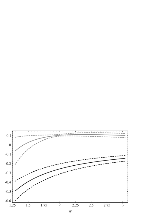
FIG. 6.: The parametrized heavy-light form factors $\theta_{1}$ (gray) and $\theta_{2}$ (black), with one standard deviation of uncertainty (with respect to the $D\rightarrow K^{*}\ell\nu$ data $V(0)$ and $A1(0)$) denoted by the dashed curves.

The relevant function for the calculation of $|V_{ts}|$ is the combination of tensor form factors $|A^{(b)}+B^{(b)}|$, as discussed in sec. 1, and defined in sec. 2. From eqns. (17) and the interpolating function displayed in fig. 6, we find

$$|A^{(b)}+B^{(b)}|(q^{2}=0)=0.78\pm 0.16\ (21\%)\ .$$ (67)

By combining the CLEO data for $B\rightarrow K^{*}\gamma$, the $B$ lifetime, and the theoretical decay rate, given in sec. 1, with this result, we find

$$\mbox{$|V_{ts}|$}=0.035\pm 0.010\ (28\%)\ .$$ (68)

Here we have quoted only the experimental uncertainty, about $21\%$ from $D\rightarrow K^{*}\ell\nu$ data, and $19\%$ from $B\rightarrow K^{*}\gamma$ data, which in turn are added in quadrature. The theoretical uncertainties are discussed in the next section.

This result compares quite well with the standard model value $\mbox{$|V_{ts}|$}=.041\pm.007\ (17\%\ {\rm total\ uncertainty})$ extracted from $V_{cb}$ and the unitarity of the CKM matrix (discussed in sec. 1). Therefore our analysis shows that the $B\rightarrow K^{*}\gamma$ data agrees with the standard model, and should be used to place constraints on non-standard model physics.

V Theoretical uncertainties and $f_{B}$

Now consider theoretical corrections to our result for $|V_{ts}|$ given by eqn. (68). We consider corrections to the heavy quark symmetry relations, to the $\alpha_{s}(m_{B})$ matching conditions, and uncertainty in the top quark mass.

The corrections to heavy quark symmetry relations are due to physics which violates the assumption that in the rest frame of the heavy meson, the heavy quark is also at rest. The first of this type is due to the QCD interactions with gluons and light quarks in the heavy meson. The correction factor is[10, 26] $\bar{\Lambda}/2m_{q}$, where $\bar{\Lambda}$ is the mass difference between the heavy meson and heavy quark. For a conservatively low value of $m_{c}=1.3$ GeV, this correction is roughly $15\%$ for the $D$ meson.

The second type of HQET correction occurs when the momentum transfer between initial and final mesons is large. Then, the emission of a hard gluon by the heavy quark before its decay can give the heavy quark a large velocity with respect to the meson rest frame. The naive estimate of this effect is[10, 11, 26] $(v\cdot{p^{\prime}})/2m_{q}\approx 1/4$ at zero $q^{2}$. However, studies of these QCD corrections indicate that the problem caused by the leading gluon exchange diagram is strongly suppressed by an order of magnitude[4, 27]. We have used the perturbative QCD calculation of sec. 3 to estimate these corrections. They are of the form

$$\Delta\theta_{1}^{(b)}=-\Delta\theta_{2}^{(b)}={w\ m_{K^{*}}\over m_{B}}C\ ,$$ (69)

where

$$C=\int_{0}^{1-\epsilon}dy{\phi^{\dagger}(y)\over\Delta_{Q}D_{G}}\ .$$ (70)

This correction comes from from the diagram of fig. (2a). We evaluated it for $\phi=\phi_{1}$ as defined in sec. 3, and plot the the ratios $\Delta\theta_{1}/\theta_{1}$, $\Delta\theta_{2}/\theta_{2}$, and $\Delta(A+B)/(A+B)$ in fig. 7.

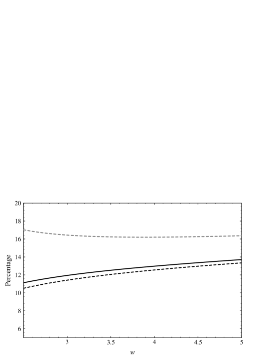
FIG. 7.: The percentage of heavy quark symmetry violating $w\ m_{K^{*}}/m_{B}$ corrections for $\theta_{1}$ (dashed gray), $\theta_{2}$ (dashed black), and $A+B$ for the $B\rightarrow K^{*}\gamma$ process (solid black).

As $w$ grows much larger than $m_{K^{*}}/m_{B}$, these corrections actually dominate the asymptotic behavior. The solid line of fig. 7 evaluated at $w=w_{B}$ gives an estimate of these corrections to $|V_{ts}|$ of about $12\%$. While the $w_{D}\ m_{K^{*}}/m_{D}$ corrections are impossible to estimate via perturbation theory because $w_{D}$ so close to one, heavy quark symmetry dictates that they should have the same form as the $w_{B}\ m_{K^{*}}/m_{B}$ corrections, that is, they are systematically correlated. The experimental values for the $\theta$’s at $w_{D}$ includes these corrections, while our perturbative analysis does not. Therefore these errors systematically compensate each other in the final result, so we use $12\%$ uncertainty total, including both corrections.

Another source of HQET violations are perturbative correction which cannot be included in the definitions of the heavy – light form factors $\theta_{i}$. From our perturbative calculation, we find that the dominant source of these corrections, which are proportional to $(1-{v\!\!\!/})/2$, are precisely the same algebraic form as the $w\cdot m_{K^{*}}/m_{B}$ corrections to the $\theta_{i}$ as discussed above. It is clearly difficult to assign a percentage of uncertainty to these corrections, since we have not calculated the precise way in which they feed into our calculation of $|V_{ts}|$, so we make a naive estimate of $6\%$ total uncertainty from them. This value is smaller than the naive estimate of $wm_{K^{*}}/m_{B}\sim 1/4$, but not by an order of magnitude as was hoped[4, 27].

We also need to estimate corrections to our perturbative QCD calculation of the matching conditions given by eqns. (58). That is, we wish to estimate the uncertainty due to the running of the form factors from $w=w_{D}$ to $w=w_{B}$. It has been suggested in the literature that the $\alpha_{s}$ contribution to the form factors may be producing only $10\%$ of the full result[4]. In this case, the matching conditions would be meaningless.

To check this, we use eqn. (51) to determine $f_{B}$. From the $D\rightarrow K^{*}\ell\nu$ data and our fits, we find

$$\kappa=f_{K^{*}}f_{B}{\sqrt{m_{K^{*}}m_{B}}\over m_{K^{*}}^{3}}{4\pi\alpha_{s}\over 9}=0.078\pm.022(28\%)\ ,$$ (71)

where we have quoted experimental uncertainties. To extract $f_{B}$ from eqn. (51), we use $\alpha_{s}(m_{B})=0.20$, and $f_{K^{*}}=212$ MeV from QCD sum rules[24]. This sum rule estimate of $f_{K^{*}}$ is supposedly is good to about $20\%$. This yields

$$f_{B}\approx 420\ {\rm MeV}.$$ (72)

This is a rather large value of $f_{B}$, when compared to numerous lattice estimates[3] of $200$ to $300$ MeV. However, it is not an order of magnitude larger than these values, which would be the case if the $\alpha_{s}$ corrections contributed only $10\%$ to the full result for the form factors. In addition, the calculation of $f_{B}$ done here assumes the leading HQET relations between the $D$ and $B$ meson systems. Decay constants are well known to receive large $1/m_{Q}$ corrections in the HQET[10], and these should be taken into account before a real prediction of $f_{B}$ is made via $D\rightarrow K^{*}\ell\nu$ and $B\rightarrow K^{*}\gamma$ data. A final note on this topic is that there is new evidence that the lattice calculations may systematically underestimate heavy quark decay constants. The recently measured[28] $f_{D_{s}}$ decay constant’s central value is about 1.5 times the central values of the lattice estimates. We conclude that the order $\alpha_{s}$ calculation is indeed dominating the form factor calculation at $w=w_{B}$. And a more proper way of calculating $f_{B}$ would be to include all $1/m_{B}$ corrections in the HQET.

Since the normalization of the form factors is set by experiment in our case, the error in $f_{B}$ is not directly correlated with error in $|V_{ts}|$. Our input for $|V_{ts}|$ from perturbative QCD are the ratios $r_{1},r_{2},r_{3}$ defined in equation (58). We currently have no systematic way of estimating their uncertainties due to higher order corrections, other that to apply that standard $\alpha_{s}/\pi$ rule for the next to leading order correction. This yields a naively small error estimate of $7\%$. Clearly, an explicit $\alpha^{2}_{s}$ calculation of the type given by Field et. al.[29] would pin this uncertainty down further. The uncertainty in $\alpha_{s}(m_{B})$ is about $10\%$. Our uncertainty in the soft physics which goes into the perturbative calculation can also be estimated. The peaking approximation for the heavy meson distribution amplitude yields about $\bar{\Lambda}/m_{B}=10\%$, and the uncertainty in the $K^{*}$ wavefunction about $m_{K^{*}}/m_{B}=17\%$.

In addition, our perturbative QCD calculation is sensitive to the IR cutoff used to regulate our perturbative momentum fraction integrals. This is the standard “solution” to the IR problem in heavy – light systems as discussed in the literature[4, 23, 30]. This aspect of the calculation definitively needs to be improved to given more confidence to the application of perturbative QCD to heavy quark systems. (Our philosophy in this paper has been to apply this “well known” QCD technology.) One way of estimating uncertainty due to this ambiguity is to perform the calculation for various distribution amplitudes. While the results were not displayed, we found that the $\phi_{czz}$ distribution amplitude gives essentially the same result for $|V_{ts}|$, to within about $10\%$ uncertainty. The similarity of the result is already evident from fig. 3. Finally, theoretical uncertainty from the top quark mass adds about $8\%$.

We combine the theoretical uncertainty into two parts. The first part consists of uncertainty due to corrections in HQET and the top quark mass. They give about $22\%$ when added in quadrature, with the dominant contributions comming from $w\cdot m_{K^{*}}/m_{Q}$ type corrections. The second type of theoretical uncertainties come from running the form factors from $w_{D}$ to $w_{B}$ via the perturbative QCD matching conditions. We estimate uncertainty of about $23\%$ from perturbative QCD uncertainties. Clearly, these are very difficult to estimate because we don’t know how the QCD corrections feed into the matching conditions eqns. (58). However, because we are using perturbative QCD rather than simply making a pole or dipole ansatz for the form factors, we can make an estimate that can be systematically improved as the perturbative calculations become more sophisticated. Hence we find a total estimated theoretical uncertainty of about $32\%$ from all sources when added in quadrature.

VI summary and conclusions

We find a value for the mixing angle of about

$$\mbox{$|V_{ts}|$}=0.035\pm.010\pm.011(28\%+32\%)$$ (73)

where the second one $\sigma$ uncertainty is a naive estimate of total theoretical errors. It is naive because it is an estimate of higher order corrections that we have not calculated. We believe that this factor can be substantially reduced by further work on $1/m_{Q}$ HQET corrections to the heavy quark matching between $D$ and $B$ systems, and an order $\alpha_{s}^{2}$ calculation of the perturbative QCD matching conditions for the heavy – light form factors at $w=w_{B}$. The most disturbing theoretical uncertainty seems, at this point, to be the IR sensitivity of the perturbative QCD calculation, which we have estimated to be $10\%$.

Our value compares very well with the standard model result[3] of $\mbox{$|V_{ts}|$}=0.041\pm.007(17\%)$, that is, our result is consistent with three generations of quarks, and the standard model contributions to the $b\rightarrow s\gamma$ penguin.

We can compare our result with recent lattice estimates of the hadronic tensor form factor for $B\rightarrow K^{*}\gamma$ decay. The UKQCD group[31] estimates $2T_{1}=|A+B|=.58^{+48}_{-56}$, and with an additional assumption of spectator mass independence, $|A+B|=.60^{+20}_{-14}$. Bernard et. al. [32] estimate $|A+B|=.40^{+04}_{-.12}$ using a pole form ansatz. These results should be compared to our result of $|A+B|=0.78\pm.16\pm.25\ (21\pm 32)\%$, where we quote separately experimental and theoretical uncertainty. (There is less experimental uncertainty than for $|V_{ts}|$ since we do not require $B\rightarrow K^{*}\gamma$ data for this parameter).

The QCD sum rule technique has also been applied to help determine the $B\rightarrow K^{*}\gamma$ form factors[33], and a single pole ansatz, with no subtractions, has been recently used[34]. As discussed in sec. 2, this ansatz is hard to reconcile with leading order HQET, so that $\bar{\Lambda}/m_{B}$ corrections play a significant role in determining the form factors by this method. However, both of these results are in rough agreement with ours.

As part of a self consistency check on the perturbative part of our analysis, we find the $B$ meson decay constant $f_{B}\approx 420$ MeV with $28\%\pm 32\%\pm 20\%$ uncertainty, where the last $20\%$ is the generic uncertainty in the $f_{K^{*}}$ decay constant from QCD sum rules. While our value of $|V_{ts}|$ is not directly correlated to this value, since we fix the normalization of our form factors from experiment, this value does indicate that the perturbative QCD calculation is correctly estimating the exclusive decay rate at large meson - meson recoil.

Appendix A: Calculation of integrals $I_{Q}$ and $I_{s}$

The QCD calculation for $\theta_{1}$, $\theta_{2}$ and $\theta_{3}$ is written in terms of two integrals over the light quark momentum fraction $y$. These integrals $I_{Q}$ and $I_{s}$ arise from the Feynman diagrams containing a heavy or strange quark propagator, figure 2a and 2b respectively. They are given by:

$$I_{Q}=\int_{\epsilon}^{1}d\bar{y}\bar{\phi}^{\dagger}_{K^{*}}(\bar{y}){m_{K^{*}}^{3}\over\Delta_{Q}D_{g}}$$

$$I_{s}=\int_{\epsilon}^{1}d\bar{y}\bar{\phi}^{\dagger}_{K^{*}}(\bar{y}){m_{K^{*}}^{3}\over\Delta_{s}D_{g}}$$

where $\Delta_{Q}$, $D_{s}$ and $D_{g}$ are given in eqns. (26) and $\bar{y}=1-y$. It is convenient to rewrite these integrals in terms of

$$I_{1}=-2wI_{Q}=\int_{\epsilon}^{1}d\bar{y}{\bar{\phi}^{\dagger}_{K^{*}}(\bar{y})\over(\bar{y}-{\bar{\Lambda}\over m_{K^{*}}w})(\bar{y}^{2}+{\bar{\Lambda}^{2}\over m_{K^{*}}^{2}}-2{\Lambda\over m_{K^{*}}}w\bar{y})}$$ (74)

and

$$I_{2}={\Delta_{s}\over m_{K^{*}}}I_{s}=\int_{\epsilon}^{1}d\bar{y}{\bar{\phi}^{\dagger}_{K^{*}}(\bar{y})\over\bar{y}^{2}+{\bar{\Lambda}^{2}\over m_{K^{*}}^{2}}-2{\Lambda\over m_{K^{*}}}w\bar{y}}$$ (75)

By partial fractions these integrals can be written in terms of a single function

$$I_{1} = {1\over a_{1}-a_{3}}{1\over a_{1}-a_{2}}(f(a_{1})-f(a_{3}))-{1\over a_{1}-a_{2}}I_{2}\ ,$$ (77)

$$I_{2} = {1\over a_{2}-a_{3}}(f(a_{2})-f(a_{3}))\ ,$$ (78)

where

$$a_{1} = {\bar{\Lambda}\over m_{K^{*}}w}\ ,$$ (80)

$$a_{2} = {\bar{\Lambda}\over m_{K^{*}}}(w+\sqrt{w^{2}-1})\ ,$$ (81)

$$a_{3} = {\bar{\Lambda}\over m_{K^{*}}}(w-\sqrt{w^{2}-1})\ ,$$ (82)

gives the position of possible poles in $1-y$, (before the Drell-Yan-West region has been cutoff), and the function $f(a_{i})$ is defined by

$$f(a_{i})=\int_{\epsilon}^{1}d\bar{y}{\bar{\phi}^{\dagger}_{K^{*}}(\bar{y})\over\bar{y}-a_{i}}\ .$$ (83)

The value of $f(a_{i})$ involves the cutoff prescription $\epsilon$ and the form of the $K{{}^{*}}$ wave function. In this paper we have employed the $w$ dependent cutoff $\epsilon={\bar{\Lambda}\over m_{K^{*}}\sqrt{w^{2}-1}}$. If the $K^{*}$ wave function is taken to be $\bar{\phi}^{\dagger}_{K^{*}}(\bar{y})=6y(1-y)$, then

$$f(a_{i})=3-6a_{i}+3\epsilon^{2}+6(a_{i}-1)\epsilon+6a_{i}(1-a_{i})\ln{|1-a_{i}|}-6a_{i}(1-a_{i})\ln{|\epsilon-a_{i}|}$$ (84)

Note that this function, together with $I_{Q}$, $I_{s}$ and $\theta_{1}$, $\theta_{2}$, $\theta_{3}$, depends only on ${\bar{\Lambda}\over m_{K^{*}}}$ and $w$, and is independent of $m_{Q}$ as required by heavy quark symmetry. The explicit form for the $\theta_{i}$ involves logarithms the largest of which goes like ${\ln{w}\over w^{2}}$ as found in the asymptotic expansions given by eqn. (30).

REFERENCES

- [1] B. Grinstein, R. Springer and M.B. Wise, Phys. Lett. B 202, 138 (1988), Nucl. Phys. B339, 269 (1990).
- [2] R. Ammar, et al., Preprint CLEO 93-06, (1993).
- [3] Particle Data Group, Phys. Rev. D 45 (1992).
- [4] G. Burdman and J.F. Donoghue, Phys. Lett. B 270 55 (1991). Note that our definition of , Eq. (1b), differs by an extra factor of from their Eq. (2).
- [5] J.L. Hewett, Phys. Rev. Lett. 70, 1045 (1993).
- [6] V. Barger, M.S. Berger, R.J.N. Phillips, Phys. Rev. Lett. 70, 1368 (1993).
- [7] R. Barbieri and G.F. Giudice, Phys. Lett. B 309, 86 (1993).
- [8] N.G. Deshpande et al., Phys. Rev. Lett. 59, 183 (1987); T. Altomari, Phys. Rev. D 37, 677 (1988); P.G. O’Donnell and H.K.K. Tung, Phys. Rev. D 44, 741 (1991).
- [9] N. Isgur and M.B. Wise, invited talk at Hadron 91, in B Physics, S. Stone (ed.), (1991) pp. 158 - 209.
- [10] M. Neubert, SLAC preprint SLAC-PUB-6263 (1993), to appear in Physics Reports.
- [11] G. Burdman, Z. Ligeti, M. Neubert, and Yosef Nir, preprint SLAC-PUB-6345 (1993).
- [12] J.D. Bjorken, SLAC-PUB-5278 (1990); A. Falk et al., Nucl. Phys. B 343, 1 (1990).
- [13] K. Kodama, et al., Phys. Rev. Lett. 66, 1819 (1991); Phys. Lett. B 263, 573 (1991); Phys. Lett. B 286, 187 (1992.)
- [14] J.C. Anjos, et al., Phys. Rev. Lett. 62, 1587 (1989); 65,2630 (1990); 67,1507 (1991).
- [15] R. Casalbuoni, et al., Phys. Lett. B 299, 139 (1993).
- [16] J.F. Amundson and J.L. Rosner, Phys. Rev. D 47, 1951 (1993).
- [17] G.P. Lepage and S.J. Brodsky, Phys. Rev. D 22, 2157 (1980).
-
[18]
G. R. Farrar and D.R. Jackson, Phys. Rev. Lett.
43, 246 (1979);
V.L. Chernyak and A.R. Zhitnitsky, JEPT Lett. 25, 510 (1977). - [19] N. Igur and M. Wise, Phys. Rev. D 42, 2388 (1990).
- [20] M.B. Voloshin and M.A. Shifman, Sov. J. Nucl. Phys. 45, 292 (1987); H.D. Politzer and M.B. Wise, Phys. Lett B 206 681 (1988).
-
[21]
A. Ali and T. Mannel, Phys. Lett. B 264, 447 (1991);
T. Ito, T. Morii, and M. Tanimoto, Phys. Lett. B 274, 449 (1992). - [22] V.I Chernyak and A.R. Zhitnitsky, Physics Reports 112, 173 (1984).
- [23] J.G. Körner and P.Kroll, Phys. Lett. B 293, 201 (1992).
- [24] V.I Chernyak, A.R. Zhitnitsky, and I.R. Zhitnitsky, Nucl. Phys. B 204, 477 (1982).
-
[25]
S.D. Drell and T.M. Yan, Phys. Rev. Lett. 24,
181 (1970);
G. West, Phys. Rev. Lett. 24, 181 (1970). - [26] A. Falk, M. Neubert, and M. Luke, Nucl. Phys. B 388, 363 (1992).
- [27] N. Isgur, Phys. Rev. D 43, 810 (1991).
- [28] CLEO Preprint CLNS 93-12-38 (1993).
- [29] R.D. Field, R. Gupta, S. Otto, and L. Chang, Nucl. Phys. B 186, 429 (1981).
- [30] A. Szczepaniak, E.M. Henley, and S.J. Brodsky, Phys. Lett. B 243, 287 (1990).
- [31] UKQCD Collaboration, Edinburgh Preprint 93/528, 1993.
- [32] C. Bernard, P. Hsieh, and A. Soni, Wash. Univ. Preprint 93-35, 1993.
- [33] P. Colangelo, C.A. Dominguez, G. Narduli, and N. Paver, Universitá Bari Preprint BARI-TH/93-150.
- [34] G. Narduli, Universitá Bari Preprint BARI-TH/93-156.