The $\epsilon$-expansion and the electroweak phase transition

Abstract

Standard perturbative (or mean field theory) techniques are not adequate for studying the finite-temperature electroweak phase transition in some cases of interest to scenarios for electroweak baryogenesis. We instead study the properties of this transition using the renormalization group and the $\epsilon$-expansion. This expansion, based on dimensional continuation from 3 to $4{-}\epsilon$ spatial dimensions, provides a systematic approximation for computing the effects of (near)-critical fluctuations. The $\epsilon$-expansion is known to predict a first-order transition in Higgs theories, even for heavy Higgs boson masses. The validity of this conclusion in the standard model is examined in detail. A variety of physical quantities are computed at leading and next-to-leading order in $\epsilon$. For moderately light Higgs masses (below 100 GeV), the $\epsilon$-expansion suggests that the transition is more strongly first order than is predicted by the conventional analysis based on the one-loop (ring-improved) effective potential. Nevertheless, the rate of baryon non-conservation after the transition is found to be larger than that given by the one-loop effective potential calculation. Detailed next-to-leading order calculations of some sample quantities suggests that the $\epsilon$-expansion is reasonably well behaved for Higgs masses below 100–200 GeV. We also compare the $\epsilon$-expansion with large-$N$ results (where $N$ is the number of scalar fields) and find that the $\epsilon$-expansion is less well behaved in this limit.

I Introduction

The electroweak phase transition has received considerable attention in the past few years because of its role in electroweak scenarios for baryogenesis [1]. Important problems include the determination of the order and strength of the phase transition as a function of the Higgs boson mass, and the calculation of the rate of baryon non-conservation near the transition. In most previous work, the principle tool for studying these problems has been the one-loop, ring-improved, finite-temperature effective potential for the Higgs field. As discussed below, the use of the ring-improved loop expansion appears untrustworthy in many applications, including the Higgs mass bounds for baryogenesis in the minimal standard model [2, 3]. The failure of the loop expansion is exactly analogous to the failure of mean field theory for describing critical behavior in condensed matter systems. One alternative method for studying critical systems, which has had considerable success in a variety of theories, is to use the $\epsilon$-expansion to improve the organization of the perturbation series. The $\epsilon$-expansion generalizes the three spatial dimensions of the theory to $4{-}\epsilon$ dimensions, solves the theory when $\epsilon$ is small, and then extrapolates to $\epsilon=1$ [4]. In this paper, we shall apply the $\epsilon$-expansion to the electroweak phase transition with the goal of estimating various parameters of the phase transition. We compute a number of observables at or near the transition including the scalar correlation length, latent heat, surface tension, free energy difference, bubble nucleation rate, and the sphaleron transition (or baryon non-conservation) rate. Next-to-leading order results are presented for the correlation length and the latent heat. We discuss in detail the expected reliability of the $\epsilon$-expansion results by (i) comparing leading and next-to-leading order contributions, (ii) comparing results of the $\epsilon$-expansion with standard perturbation theory in the limit of a small Higgs mass (where the ordinary loop expansion remains reliable), and (iii) comparing $\epsilon$-expansion results when the number of scalar fields is large to direct large-$N$ calculations.

In the remainder of the introduction, we review the need for detailed knowledge of the electroweak phase transition in order to determine the viability of electroweak baryogenesis scenarios, and discuss the reliability of the standard loop expansion. Then we briefly sketch the rather successful $\epsilon$-expansion results for critical behavior in simple $\phi^{4}$ theories, present an overview of the application of the $\epsilon$-expansion to the standard electroweak theory, and discuss some possible pitfalls of this approach. We also review the existence of a non-perturbative magnetic mass in SU(2) theory and discuss its implications for the $\epsilon$-expansion. Detailed calculations follow in subsequent sections, which will be outlined later in this introduction.

A Motivation

One of Sakharov’s three famous requirements for baryogenesis is that the universe be out of equilibrium. In electroweak scenarios, baryogenesis occurs during the electroweak phase transition and Sakharov’s condition is met if that transition is first order rather than second order. First-order transitions proceed by the nucleation, expansion, and coalescence of bubbles of the new phase inside the old—a highly non-equilibrium process. However, the phase transition must not merely be first order, it must be sufficiently strongly first order. In particular, one constraint arises from considering the rate of baryon number violation at the end of the phase transition, when baryogenesis is completed. This rate is exponentially sensitive to the expectation value $\langle\phi\rangle$ of the Higgs field responsible for symmetry breaking, behaving as $\Gamma_{\rm B}\sim\exp\{-({\rm const.})\beta\langle\phi\rangle/g\}$, where $\beta$ is the inverse temperature and $g$ the electroweak coupling. If $\langle\phi\rangle$ is too small after the phase transition, then baryon-number violation continues unabated after baryogenesis and the universe relaxes back to an equilibrium state of zero net baryon number. Any successful scenario requires that $\langle\phi\rangle$ be sufficiently large at the end of the transition so that baryon number violation is effectively shut off. Thus, one important goal of studies of the electroweak phase transition has been to determine the strength of the transition, as measured by the size of the discontinuity in $\langle\phi\rangle$ across the transition.

These issues have been previously studied using the one-loop ring-improved finite-temperature potential for the Higgs field $\phi$. With this approximation to the potential, one finds a first-order phase transition and the Higgs expectation value immediately after the transition can easily be evaluated. In particular, one may study the strength of the transition in the simplest interesting model: the minimal standard model with a single Higgs doublet. This is presumably only a toy model because, unlike multiple-Higgs models, it is unclear whether the minimal model incorporates sufficient CP violation for baryogenesis. Nevertheless, because of its small set of unknown parameters, the minimal model provides a relatively uncluttered testing ground for techniques used to analyze the phase transition. In this model, employing the one-loop ring-improved potential, Dine et al.[2] found that baryon number violation is turned off at the end of baryogenesis only if the zero-temperature Higgs mass $m_{\rm h}(0)$ is less than 35 to 40 GeV. A successful scenario for electroweak baryogenesis is then incompatible with the experimental limit $m_{\rm h}(0)>60$ GeV.

This disaster is avoidable in multiple-Higgs models, but in any model it will be important to understand the reliability of predictions based on the one-loop potential. So let us stick with the minimal model and review the reliability of the above constraints. The loop expansion parameter at high temperature is not simply $g^{2}$ but rather $g^{2}T/M$, where the characteristic mass scale is set by the $W$-boson mass (at temperature $T$), $M\sim g\phi$. Computing $M$ at the phase transition, one finds that the loop expansion parameter $g^{2}T/M$ is of order $\lambda/g^{2}$. (A review of this power counting may be found in section 2 of Ref. [5].) Hence, the loop expansion breaks down, and calculations based on the one-loop potential are unreliable, unless $\lambda\ll g^{2}$; that is, unless the Higgs mass $m_{\rm h}(0)$ at zero temperature is much less than the $W$-mass $M_{\rm W}(0)$. This criteria is not obviously satisfied by the $m_{\rm h}(0)$ bound of 35 to 40 GeV found by Dine et al., and the importance of higher-order corrections will be determined by all the detailed numerical factors left out of this facile estimate of the loop expansion parameter. To test the reliability of the one-loop results, two-loop corrections to the potential were computed in Refs. [5, 7] and are displayed at the critical temperature in Fig. 1 for $m_{\rm h}(0)=35$ GeV and a top quark mass $m_{\rm t}(0)=110$ GeV. Computed in Landau gauge, $\langle\phi\rangle$ increases by only 20% when two-loop corrections are included. But the height of the barrier in the potential increases by a factor of almost three! This dramatic change in the height suggests that the loop expansion is unreliable. One might optimistically hope that the correction to the logarithm of the baryon violation rate $\Gamma_{\rm B}$ will be small because $\ln\Gamma_{\rm B}$ is proportional to $\langle\phi\rangle$, which has a relatively small two-loop correction. However, this proportionality is only valid at leading order, and $\ln\Gamma_{\rm B}$ has its own, independent corrections controlled by $\lambda/g^{2}$. There is no obvious reason why these corrections might not be numerically large, similar to the correction to the hump in the potential.

FIG. 1.: The effective potential at the critical temperature for $m_{\rm h}(0)$ = 35 GeV and $m_{\rm t}(0)$ = 110 GeV. The dashed and solid lines are the one-loop and two-loop results respectively.

Because of these problems with the loop expansion, it is clearly appropriate to explore other techniques, such as the $\epsilon$-expansion, for studying the electroweak phase transition.

B A success story: pure scalar theory.

Before discussing the electroweak theory, it will be useful to review briefly the $\epsilon$-expansion in a much simpler model where it enjoys some success. Consider a real scalar field theory in $3+1$ spacetime dimensions at temperature $T$, with the Euclidean Lagrangian

$${\cal L}_{\rm E}={\textstyle{1\over 2}}(\partial\phi)^{2}-{\textstyle{1\over 2}}\nu^{2}\phi^{2}+{\textstyle{1\over 4!}}\lambda\phi^{4}\,.$$ (1)

One could attempt to analyze the phase transition by computing the one-loop ring-improved potential. With this approximation one would predict a first-order phase transition. However, this computation also yields a loop expansion parameter $\lambda T/m_{\rm eff}(T)$ of order 1 at the transition, and so the one-loop result cannot be trusted. In fact, this model is in the same universality class as the Ising model and is known to have a second-order phase transition.

The $\epsilon$-expansion analysis of this transition is well known and proceeds as follows. The study of a second-order phase transition requires exploring the infrared behavior of the theory. In the Euclidean formulation of equilibrium finite-temperature quantum field theory, space-time is periodic in the time direction with period $\beta\equiv 1/T$. For spatial distances $r$ large compared to $\beta$, fluctuations in the Euclidean time direction are irrelevant and the theory reduces to an effective three-dimensional theory. Up to corrections suppressed by powers of $\beta/r$, the only effect of decoupled temporal fluctuations is to renormalize the parameters of the three dimensional theory, i.e., masses and coupling constants, from their original four-dimensional values. The relationship between the three- and four-dimensional parameters is perturbatively calculable. In the case at hand, one finds that the mass parameters in the three- and four-dimensional theories are related by

$$m^{2}=-\nu^{2}+{\textstyle{1\over 24}}\,\lambda T^{2}+O(\lambda\nu^{2},\lambda^{2}T^{2})\,.$$ (2)

The second term is the standard one-loop thermal contribution to the mass and is responsible for the phase transition. By adjusting $T$, one can approach the phase transition by tuning the mass $m$ of the three-dimensional theory toward zero. The study of second-order (or weakly first-order) phase transitions is therefore the study of the infrared behavior of three-dimensional theories.

FIG. 2.: The renormalization group flow in $\lambda\phi^{4}$ theory.

Now consider this theory in $d=4{-}\epsilon$ spatial dimensions, instead of 3, where $\epsilon$ is finite but small compared to 1. The infrared behavior can be studied by following the flow of relevant couplings using the renormalization group (RG). For a scalar theory, one has

$$\mu{d\over d\mu}\lambda(\mu)=-\epsilon\lambda+\beta(\lambda).$$ (3)

The first term, which vanishes in the four-dimensional limit, reflects the trivial classical scaling arising from the fact that the interaction $\int d^{d}x\,\phi^{4}$ has engineering dimension $-\epsilon$. The function $\beta(\lambda)$ is the usual four-dimensional $\beta$-function given perturbatively by

$$\beta(\lambda)={3\over(4\pi)^{2}}\,\lambda^{2}+O(\lambda^{3})\,.$$ (4)

The renormalization group flow is depicted qualitatively in Fig. 2, where the arrows denote flows into the infrared (i.e., decreasing $\mu$). There is an infrared-stable fixed point at

$$\lambda_{*}={(4\pi)^{2}\!\over 3}\,\epsilon+O(\epsilon^{2})\,.$$ (5)

Such a fixed point indicates a second-order phase transition since, if the temperature has been adjusted so that $m$ is zero, the behavior of the theory at the fixed point in $\lambda$ will then look the same on all distance scales.

Note that the fixed point coupling is small, $\lambda\ll 1$, provided that $\epsilon\ll 1$. For this reason, the one-loop result for the $\beta$-function (4) is sufficient to find the fixed-point to leading order in $\epsilon$. Renormalization-group improved perturbation theory in $\lambda$ is therefore equivalent to an expansion in powers of $\epsilon$. It is for this reason that calculations of the phase transition are more tractable in $4{-}\epsilon$ dimensions, when $\epsilon$ is small, than in three dimensions.

By computing anomalous dimensions of various operators at the fixed point, one can extract the critical exponents associated with the phase transition. For instance, one finds in a three-loop calculation that the susceptibility exponent $\gamma$, defined by $\chi\sim|T-T_{\rm c}|^{\gamma}$ where $\chi$ is the susceptibility, is given by [4, 10]

$$\gamma=1+0.167\,\epsilon+0.077\,\epsilon^{2}-0.049\,\epsilon^{3}+O(\epsilon^{4})\,.$$ (6)

Perturbation expansions are asymptotic in $\lambda$, and the terms in the expansion start growing in magnitude at orders $n\,\,\vbox{\hbox{$\buildrel\displaystyle>\over{\sim}$}}\,\,O(1/\lambda)$. Expansions in $\epsilon$ are therefore also asymptotic, with terms growing in magnitude at orders $n\,\,\vbox{\hbox{$\buildrel\displaystyle>\over{\sim}$}}\,\,O(1/\epsilon)$. What does this imply when one finally returns to the three-dimensional theory by sending $\epsilon\to 1$? If one is lucky, $O(1/\epsilon)$ really means something like three or four when $\epsilon=1$ and the first few terms of the series will be useful. If one is unlucky, no terms in the expansion will be useful. Whether or not one will be lucky cannot be determined in advance of an actual calculation. From the result (6), we see that the terms displayed do indeed get smaller for $\epsilon=1$, and their sum in 1.195. This compares favorably with results determined by high-order Borel resummation techniques[11], which give $1.2405\pm 0.0015$. (This value is consistent with numerical results using lattice methods[12].) So the straightforward use of the $\epsilon$-expansion above appears to get within 4% of the true answer—a stunning achievement.

Another example, which isn’t quite as nicely behaved, is the anomalous dimension $\eta$ of the two-point correlation function, defined by $\langle\phi(r)\phi(0)\rangle\sim r^{2-d-\eta}$. Because its leading order contribution happens to vanish, the exponent $\eta$ is a small number. One finds [4, 13]

$$\eta=0.0185\,\epsilon^{2}+0.0187\,\epsilon^{3}-0.0083\,\epsilon^{4}+0.0359\,\epsilon^{5}+O(\epsilon^{6})\,.$$ (7)

If one takes $\epsilon\to 1$ and adds terms until they start increasing, one obtains $\eta=0.0289$. The correct answer is believed to be $\eta\approx 0.035$ [11, 12].

C Electroweak theory

We now turn to the application of the $\epsilon$-expansion to electroweak theory. We shall ignore the Weinberg mixing angle, and concentrate on an SU(2) gauge theory with a single complex Higgs doublet. One must first reduce the theory to an effective three-dimensional one, and then map out the renormalization group flows in $4{-}\epsilon$ dimensions. This procedure has been analyzed by Ginsparg for general non-Abelian gauge theories [17]. When constructing the three-dimensional theory, one finds that the $A_{0}$ component of the four-dimensional gauge field picks up a Debye screening mass of order $gT$. The three-dimensional theory then consists of the SU(2) Higgs doublet $\Phi(\vec{x})$, a three-dimensional SU(2) gauge field $\vec{A}(\vec{x})$, and a massive scalar $A_{0}(\vec{x})$ that is in the adjoint representation of SU(2). We are interested in the infrared behavior of the theory, however, and the massive $A_{0}$ field will decouple from distance scales large compared to $1/gT$. One may integrate out its effects as well, leaving a three-dimensional SU(2)-Higgs theory of $\Phi$ and $\vec{A}$.

Now consider instead a $4{-}\epsilon$ dimensional SU(2)-Higgs theory. The one-loop renormalization group equations have the form

$$\mu{dg^{2}\over d\mu} = -\epsilon\,g^{2}+\hat{\beta}_{0}\,g^{4},$$ (9)

$$\mu{d\lambda\over d\mu} = -\epsilon\,\lambda+(\hat{a}\,g^{4}+\hat{b}\,g^{2}\lambda+\hat{c}\,\lambda^{2}).$$ (10)

The precise numerical coefficients, as well as the explicit solution, will be given in section 2. One finds that the flows have the form shown in Fig. 3. There is no infrared stable fixed point, and all trajectories flow to the region $\lambda<0$ where the Higgs sector appears to become unstable. This instability, and the absence of stable fixed points, suggest that the phase transition is always first-order in $4{-}\epsilon$ dimensions [17].

FIG. 3.: The renormalization group flow for an SU(2)-Higgs theory. The dashed line is the trajectory which flows from the initial couplings $(g_{1}^{2},\lambda_{1})$ into the region where $\lambda\ll g^{2}$.

The last point deserves more careful analysis, which can be provided by recalling the previous discussion of the one-loop effective potential. Notice that, although the couplings may start at a point $(g_{1}^{2},\lambda_{1})$ where the naive loop expansion parameter $\lambda/g^{2}$ is not small, they eventually flow into the region $\lambda\ll g^{2}$. At this point one can apply the familiar analysis based on computing the effective potential. As we shall see, the phase transition is indeed first-order when $\epsilon$ is small and its properties can be reliably computed.

In order to make contact with $\epsilon=1$, it is useful to consider how Fig. 3 changes with $\epsilon$. The one-loop renormalization group equations have the interesting property that the trajectories in the ($g^{2}$,$\lambda$) plane are independent of $\epsilon$ if $g^{2}$ and $\lambda$ are rescaled by $\epsilon$, but the rate at which those trajectories are traversed is exponentially sensitive to $\epsilon$. Specifically, by rewriting

$$g^{2}\equiv\epsilon\,\tilde{g}^{2},\qquad\lambda\equiv\epsilon\,\tilde{\lambda},\qquad\mu\equiv\tilde{\mu}^{1/\epsilon},$$ (11)

the equations become independent of $\epsilon$,

$$\tilde{\mu}{d\tilde{g}^{2}\over d\tilde{\mu}} = -\tilde{g}^{2}+\hat{\beta}_{0}\,\tilde{g}^{4},$$ (13)

$$\tilde{\mu}{d\tilde{\lambda}\over d\tilde{\mu}} = -\tilde{\lambda}+(\hat{a}\,\tilde{g}^{4}+\hat{b}\,\tilde{g}^{2}\tilde{\lambda}+\hat{c}\,\tilde{\lambda}^{2})\,.$$ (14)

Hence, for these one-loop equations, Fig. 3 does not change with $\epsilon$ provided we label the axes as $g^{2}/\epsilon$ and $\lambda/\epsilon$.

We are now in a position to outline our basic approach for using the $\epsilon$-expansion to compute quantities associated with the phase transition. This approach is closely related to the methods used years ago by Chen, Lubensky, and Nelson to study U(1)-Higgs theory (i.e., superconductivity) [18] and before that by Rudnick to study the cubic anisotropy model [15]. Start by considering the original four dimensional theory and the effective three dimensional theory, regulating both with dimensional regularization and renormalizing at the scale $\mu_{1}=T$. Relate the three dimensional couplings to the four dimensional ones by computing perturbatively, in both theories, physical quantities characterized by the momentum scale $T$ and equating the results. For example, one can compute the four-point scalar amplitude when the external momenta are of order $T$. One finds a perturbative relation between the three- and four-dimensional couplings which is trivial at leading order:

$$g_{1}^{2} = \bar{g}^{2}(T)+O(\bar{g}^{3}),\qquad$$ (16)

$$\lambda_{1} = \bar{\lambda}(T)+O(\bar{g}^{3},\bar{\lambda}^{2}).$$ (17)

Here, $g_{1}^{2}$ and $\lambda_{1}$ are the three-dimensional couplings at a scale $\mu_{1}=T$, and $\bar{g}^{2}$ and $\bar{\lambda}$ are the couplings of the original 4-dimensional theory. The three dimensional couplings $g_{1}^{2}$ and $\lambda_{1}$ are the starting points for the renormalization group flow depicted in Fig. 3. Now go from three to $4{-}\epsilon$ dimensions while holding $g_{1}^{2}/\epsilon$ and $\lambda_{1}/\epsilon$ fixed, so that the relative position in Fig. 3 does not change. Finally, use the renormalization group to flow to an equivalent theory in the region $\lambda\ll g^{2}$. The phase transition in this theory can now be studied using a loop expansion to compute the effective potential. Note that, for small $\epsilon$, scaling the couplings $g_{1}^{2}$ and $\lambda_{1}$ to be $O(\epsilon)$ while holding $\lambda_{1}/g_{1}^{2}$ fixed, automatically implies that $g_{1}^{4}\ll\lambda_{1}\ll 1$.

In this paper, we shall not concern ourselves with the calculational details of the higher-order matching (I C) of the three-dimensional couplings with the original four-dimensional ones. We shall instead focus on the infrared behavior of the three-dimensional theory as predicted by the $\epsilon$-expansion. This is appropriate if the original four-dimensional couplings $\bar{g}^{2}$ and $\bar{\lambda}$ are taken to be very small while the ratio $\bar{\lambda}/\bar{g}^{2}$ is held fixed. So we shall study the limit

$$\bar{g}^{2},\bar{\lambda}\rightarrow 0,\qquad\hbox{with}\qquad{\bar{\lambda}/\bar{g}^{2}}~{}\hbox{fixed}.$$ (18)

In practice, this means that we will assume that $\bar{\lambda}\sim\bar{g}^{2}\ll 1$ but $\lambda\gg g^{3},~{}g^{4},$ etc. This is appropriate for the real electroweak theory if the Higgs mass is small compared to 1 TeV but not much smaller than the W-mass. We make this assumption that the couplings are small only to simplify the relationship between the four- and three-dimensional theories. When working within the three-dimensional theory itself, however, we shall generally present formulas that are valid even when $g_{1}^{2}$ and $\lambda_{1}$ are not assumed small.

D Outline

Our presentation in section II begins with the one loop analysis. The explicit solution of the one-loop renormalization group flow equations is presented, followed by the evaluation of the one-loop effective potential (in $4{-}\epsilon$ dimensions) when the scalar self-coupling vanishes. This information is then used to compute, to one-loop order within the $\epsilon$-expansion, the scalar correlation length at the phase transition in both the symmetric and asymmetric phases, the baryon violation and bubble nucleation rates at the transition, the latent heat of the transition, surface tension, and the free energy difference between symmetric and asymmetric phases near the transition. The predictions of the $\epsilon$-expansion for these physical quantities are then compared to the results obtained from one-loop perturbation theory directly in three dimensions, in the limit where $\lambda\ll g^{2}$.

Section III contains two loop analysis. The two-loop renormalization group equations are presented, along with their explicit solutions, followed by the two-loop effective potential for $\lambda=0$. Two-loop corrections to the scalar correlation length and latent heat are computed. We again compare results with direct three-dimensional perturbation theory in the $\lambda\ll g^{2}$ limit. More significantly, by examining the relative size of the two-loop corrections, we can test whether the $\epsilon$-expansion is well-behaved in the case $\lambda\,\,\vbox{\hbox{$\buildrel\displaystyle>\over{\sim}$}}\,\,g^{2}$ of moderate-to-heavy Higgs mass, where conventional perturbation theory fails.

Section IV examines the $\epsilon$-expansion when one increases the number of scalar fields, $N$. Near four dimensions, when the number of charged scalar fields is sufficiently large ($N>N_{\rm c}$), two additional renormalization group fixed points appear: an infrared stable fixed point and a tricritical point. We compute the first two terms in the $\epsilon$-expansion of the critical value $N_{\rm c}$ at which these fixed points first appear. We also examine the $N\to\infty$ limit of the slope $\lambda/g^{2}$ of the tricritical line separating theories with first and second order transitions, and compare the $\epsilon$-expansion result with that obtained directly in three-dimensions using large-$N$ methods.

The overall interpretation of our results is summarized in the conclusion. Various details of two-loop calculations are relegated to appendices.

E Possible Misgivings

Before embarking on explicit calculations using the $\epsilon$-expansion, it is worth considering whether the endeavor is doomed before it begins. In particular, the $\epsilon$-expansion predicts that the phase transition is always first order, even when $\lambda_{1}/g_{1}^{2}$ is arbitrarily large. Some authors have dismissed this result based on the apparent failure of analogous arguments for superconductivity. At large distances, simple superconductors are described by Landau-Ginzburg theory, which is just U(1) gauge theory with a single, charged, complex scalar field. The renormalization group equations in $4{-}\epsilon$ dimensions have the same form as Eq. (I C) with $\beta_{0}$ positive. The flow is shown in Fig. 4. As observed by Halperin et al., [21], the $\epsilon$-expansion predicts the superconducting phase transition to be always first order, even deep in the Type II regime, $\lambda_{1}\gg g_{1}^{2}$.

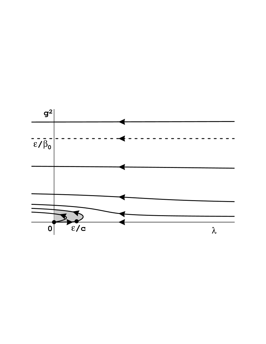
FIG. 4.: The renormalization group flow for a U(1)-Higgs theory with $N<N_{\rm c}$.

The predicted strength of the transition is too small to measure in superconductors, but detailed studies have been made of the critical properties of smectic-A liquid crystals, which are argued to be in the same universality class as superconductors [22]. The predicted first-order transition is often not observed. Motivated by this discrepancy, Dasgupta and Halperin [23] made a lattice study of the superconducting transition. They used a U(1) lattice gauge theory in three dimensions with a fixed-length Higgs field; that is, their bare theory had $\lambda_{1}\to\infty$ with $m^{2}/\lambda_{1}$ fixed. Simulating a bare theory that had $g_{1}^{2}=5$, they found no numerical evidence of a first-order phase transition.

Their numerical results are not ironclad. The height of the specific heat peak was measured on lattices of size $3^{3}$, $5^{3}$, $10^{3}$, and $15^{3}$. In a first-order phase transition, the height should grow like the volume ${\cal V}$ in the large-volume limit; for a second-order transition, it should grow like ${\cal V}^{2\alpha/3}$ (or $\ln{\cal V}$ if the specific heat exponent $\alpha\approx 0$) [23]. Results on these four lattice sizes did not support a linear relationship between the height and ${\cal V}$. However it is not clear if these simulations reached the large volume limit. As a rough guide, one may consider the predictions of the $\epsilon$-expansion. If we use the one-loop flows and set $\epsilon=1$, we find that the scale change necessary for the initial theory with $\lambda_{1}=\infty$ and $g_{1}^{2}=5$ to run to the region $\lambda<0$ is roughly 9. (Detailed formulas are given in section 2.) This suggests that the width of domain walls, or the minimal size of critical bubbles nucleated in a first-order phase transition, will be of order $9$ lattice units. Therefore, the linear growth of the specific-heat peak with ${\cal V}$ need not begin until the lattice size is larger than $O(9^{3})$. Given that the lattices of [23] range in size from $3^{3}$ to $15^{3}$, the reliability of the conclusions is clearly sensitive to whether the condition ${\cal V}\gg O(9^{3})$ really means something like ${\cal V}\geq 4^{3}$ versus something like ${\cal V}\geq 18^{3}$.

Nevertheless, given the other evidence from liquid crystals, let us put this concern aside and hypothesize that the phase transition studied in [23] is in fact second order. The presence of a continuous transition in a fixed-length U(1)-Higgs theory would imply that the $\epsilon$-expansion does a terrible job describing the flow of theories starting near $\lambda_{1}=\infty$. These theories must flow to some infrared-stable fixed point not seen within the $\epsilon$-expansion. However, as noted after Eq. (18), in the application to electroweak theory one is interested not in theories that start at strong coupling with $\lambda_{1}=\infty$, but in perturbative theories that start near the unstable Gaussian fixed point at $\lambda=g^{2}=0$. The latter theories need not lie within the domain of attraction of the putative fixed point, and might instead be correctly described by the $\epsilon$-expansion. Within the $\epsilon$-expansion, all theories which start near $\lambda=g^{2}=0$ stay inside the shaded region of Fig. 4. Recall that at leading order the $\epsilon$-expansion is based on renormalization-group improved one-loop perturbation theory. One way to view the success of the $\epsilon$-expansion in pure $\lambda\phi^{4}$ theory is to note that, even though the fixed point coupling $\lambda$ is formally $O(1)$ when $\epsilon\to 1$, the coupling is not such a large number that higher-order corrections in $\lambda$ cause dramatic changes. If we are similarly lucky, the couplings in the shaded region of Fig. 4 will not be so large when $\epsilon\to 1$ as to render the $\epsilon$-expansion useless.

FIG. 5.: The renormalization group flow for a U(1)-Higgs theory with $N>N_{\rm c}$. Point $A$ is an infrared-stable fixed point, while $B$ is a tricritical point. The dashed line is the tricritical line which separates theories with first and second order transitions.

An important general point is that phase transitions are more likely to be second order in lower dimensions due to the increased importance of long-distance fluctuations. A prediction of a second-order phase transition in $4{-}\epsilon$ dimensions may be more robust as $\epsilon\to 1$ than a prediction of a first-order phase transition. A useful setting for discussing this point is provided by the generalization of the single scalar U(1)-Higgs theory to a theory of $N$ charged scalars with a global U($N$) symmetry. For $N$ very large, one finds that the flow looks like Fig. 5 instead of Fig. 4. An infrared-stable fixed point and a tricritical point have appeared. Theories which start to the right of the dashed line have second-order phase transitions; those to the left undergo first-order transitions. Near four dimensions, the transition between Fig. 4 and Fig. 5 occurs at $N_{\rm c}(4)=183.0$. As the dimension $d$ is decreased and second-order transitions become more likely, the critical number of fields, $N_{\rm c}(d)$, should decrease. We would like to know whether $N_{\rm c}(3)<1$.

In section IV, we compute the first sub-leading correction to $N_{\rm c}$ within the $\epsilon$-expansion. This is only a computation of the slope of $N_{\rm c}(d)$ near $d=4$. However, for both U(1) and SU(2), when extrapolated to $\epsilon=1$, we find that the $O(\epsilon)$ term is larger than the leading order term and of opposite sign, so that $N_{\rm c}$ naively extrapolates to $N_{\rm c}(3)<1$. But one cannot trust this result because the series is clearly badly behaved. This in itself is somewhat discouraging because $N_{\rm c}$ is revealed to be an example of a physical quantity for which the $\epsilon$-expansion is not very well behaved.

We do not believe that there is any compelling evidence one way or the other as to whether the SU(2) phase transition, with one Higgs doublet, is first or second order for large Higgs mass. This is an issue to be resolved by lattice simulations or other techniques. If it is second order for large or moderate $\lambda_{1}/g_{1}^{2}$, then the $\epsilon$-expansion is doomed. Our philosophy will be to assume that the transition is indeed first-order and see what we can extract from the $\epsilon$-expansion.

Before closing this section, we note one other hurdle for the $\epsilon$-expansion posed by recent literature. One can solve the U(1) and SU(2) theories directly in three dimensions in the limit $N\to\infty$. Alternatively, one can compute to some finite order in the $\epsilon$-expansion, set $\epsilon=1$, and only then take the $N\to\infty$ limit of the result. A comparison of the two results gives a test of the $\epsilon$-expansion. In particular, one can compute the value of $\lambda/g^{2}$ for the line that divides first- from second-order transitions. This has been investigated in the large-$N$ expansion by Jain et al.[25]. Their result is completely different from that suggested by the $\epsilon$-expansion, differing even in the power of $N$. In section IV, we discuss the flaw in their analysis and redo their calculation. We find that the critical value of $\lambda/g^{2}$ scales like $1/N$ as $N\to\infty$ and that this behavior is in agreement with the $\epsilon$-expansion.

F The magnetic mass and non-perturbative physics

It is well known that unbroken non-Abelian gauge theories at high temperature (such as SU(2) electroweak theory in the symmetric $\phi=0$ phase) suffer a breakdown of perturbation theory beyond the first few orders. The loop expansion parameter is not just large; it is infrared divergent. This reflects the fundamentally non-perturbative nature of long distance physics in these theories. In this section, we discuss how this affects the $\epsilon$-expansion.

FIG. 6.: An example of an infrared divergent contribution to the transverse gauge field mass in three dimensions.

An easy way to see the problem is to study the effective three-dimensional theory and attempt to compute the transverse gauge field mass in perturbation theory. Gauge invariance and rotational invariance imply that the self-energy of the gauge field $\vec{A}$ should have the form

$$\Pi_{ij}(\vec{p}\,)=(\vec{p}^{\>2}\delta_{ij}-p_{i}p_{j})f(\vec{p}^{\>2})\,.$$ (19)

Unless $f(\vec{p}^{\>2})$ singular as $\vec{p}^{\>2}\rightarrow 0$, there will be no mass at any order in perturbation theory. However, fig. 6 shows a self energy graph which is infrared divergent. This divergence can be seen using simple three-dimensional power counting which shows this diagram gives the logarithmically-divergent contribution

$$g_{1}^{4}T^{2}\int{{\rm d}^{6}k\over k^{6}},$$ (20)

at zero external momentum. Higher order diagrams have increasingly severe divergences. Non-perturbative fluctuations produce a finite correlation length which serves to cut-off these divergences. The inverse correlation length (or magnetic mass) is of order $g_{1}^{2}T$ (or $g^{2}\mu$). If one now computes a three-loop diagram using this scale as an infrared cut-off, one finds a contribution of order

$$g_{1}^{6}T^{4}\int\nolimits_{g_{1}^{2}T}{{\rm d}^{9}p\over p^{10}}\sim g_{1}^{4}T^{2}.$$ (21)

This is the same size as the two-loop diagram, as are all higher-loop contributions! Perturbation theory is therefore inadequate to treat infrared physics at scales of order $g_{1}^{2}T$.

What happens to this problem in $4{-}\epsilon$ dimensions? The two-loop diagram of fig. 6 is no longer infrared divergent when $\epsilon<1$, and infrared problems do not arise until higher order. In particular, an $n$-loop contribution has the form

$$(g^{2}\mu^{\epsilon})^{n}\int{{\rm d}^{4-\epsilon}p\over p^{4n-2}}\,,$$ (22)

so that infrared divergences first appear at order $n=2/\epsilon$. Perturbation theory is useless beyond this order, which means that no quantity can be computed perturbatively with relative error smaller than $g^{n}=g^{2/\epsilon}$. Since $g^{2}$ is $O(\epsilon)$ in our procedure for the $\epsilon$-expansion, this relative error is $[O(\epsilon)]^{1/\epsilon}$. But this is just the same order as the uncertainty intrinsic to the $\epsilon$-expansion in any theory due to the fact that the expansion in $\epsilon$ is an asymptotic series; terms of order $\epsilon^{k}$ in the series start getting larger beyond order $k\sim 1/\epsilon$. So the non-perturbative physics related to the mass gap in three-dimensional non-Abelian gauge theories may not pose any problem for the $\epsilon$-expansion not already present from the asymptotic nature of the expansion.

Some physical quantities we will examine are infrared-safe as they depend only on physics in the asymmetric phase (where all particles have perturbative masses), or do not probe the symmetric phase over long distances. Other quantities, such as the scalar correlation length in the symmetric phase are, in three dimensions, infrared safe at lowest order but not at higher orders. How well the $\epsilon$-expansion will work, after extrapolating $\epsilon\to 1$, for such quantities remains unclear. This issue will be discussed further in section III C. We will, however, largely focus on infrared-safe quantities when computing beyond leading order.

II One-loop analysis

A Renormalization group flow

We are now ready to look in detail at the solutions to the one-loop renormalization-group equations. We shall quote results for both U(1) gauge theory with $N$ charged U($N$)-symmetric scalars, and SU(2) gauge theory with $N/2$ U($N/2$)-symmetric scalar doublets. $N$ will always denote the number of complex scalar degrees of freedom. The Lagrangians are

$${\cal L}_{\rm E}^{\rm U(1)} = {\textstyle{1\over 2}}\left|(\partial-i\mu^{\epsilon/2}gA)\vec{\Phi}\right|^{2}+{\textstyle{1\over 2}}\,m^{2}|\vec{\Phi}|^{2}+{\textstyle{1\over 4!}}\,\mu^{\epsilon}\lambda|\vec{\Phi}|^{4}+{\textstyle{1\over 4}}\,F_{\mu\nu}^{2}\,,$$ (24)

$${\cal L}_{\rm E}^{\rm SU(2)} = {\textstyle{1\over 2}}\left|(\partial-i\mu^{\epsilon/2}gA^{a}\tau_{a}/2)\vec{\Phi}\right|^{2}+{\textstyle{1\over 2}}\,m^{2}|\vec{\Phi}|^{2}+{\textstyle{1\over 4!}}\,\mu^{\epsilon}\lambda|\vec{\Phi}|^{4}+{\textstyle{1\over 4}}\,\left(F^{a}_{\mu\nu}\right)^{2}.$$ (25)

We will express potentials in terms of the scalar field modulus $\phi=|\vec{\Phi}|\equiv(\sum_{a}\Phi_{a}^{2})^{1/2}$, in terms of which the classical potential takes the canonical form,

$$V(\phi)={\textstyle{1\over 2}}\,m^{2}\phi^{2}+{\textstyle{1\over 4!}}\,\mu^{\epsilon}\lambda\,\phi^{4}\,.$$ (26)

We choose couplings $\lambda$ and $g^{2}$ to be dimensionless in any spacetime dimension and therefore need to include explicit powers of the renormalization point $\mu$ in the interaction terms.

The renormalization group will be used to run from a renormalization point $\mu_{1}=T$ to a final scale $\mu$. Our notation will later be more compact if we write $\mu=\mu_{1}/s$, where $s$ starts at 1 and grows to $\infty$ as one flows into the infrared. In place of the gauge couplings in (II A) with standard normalizations, it will also be convenient to use the “charge”,

$$q\equiv\cases{g,&{\rm U(1)}\cr g/2,&{\rm SU(2)} .}$$ (27)

The mass of the gauge boson is then $q\mu^{\epsilon}\phi$ in both theories. The introduction of the charge $q$ will allow us to write common expressions for most one-loop results in either gauge theory. The one-loop RG equations take the form

$$s{dq^{2}\over ds} = \epsilon\,q^{2}-\beta_{0}\,q^{4}\,,$$ (29)

$$s{d\lambda\over ds} = \epsilon\,\lambda-(a\,q^{4}+b\,q^{2}\lambda+c\,\lambda^{2})\,,$$ (30)

where the constants are given by

$$\beta_{0}={2(N-44\,C_{2})\over 3(4\pi)^{2}}\,,\qquad a={36\,n_{\rm g}\over(4\pi)^{2}}\,,\qquad b=-{12\,n_{\rm g}\over(4\pi)^{2}}\,,\qquad c={2(N+4)\over 3(4\pi)^{2}}\,,$$ (31)

where

$$n_{\rm g}\equiv\cases{1,&{\rm U(1)} ;\cr 3,&{\rm SU(2)} ,}\qquad$$ (32)

is the number of gauge bosons. $C_{2}$ is the quadratic Casimir which, for our two gauge groups of interest, equals $n_{\rm g}-1$. We shall later also need the renormalization group equation for the mass $m^{2}$,

$$s{dm^{2}\over ds}=-(l_{0}\,q^{2}+l_{1}\,\lambda)\,m^{2}\,,$$ (33)

where

$$l_{0}=-{6\,n_{\rm g}\over(4\pi)^{2}}\,,\qquad l_{1}={2(N+1)\over 3(4\pi)^{2}}\,.$$ (34)

We shall not need the renormalization group equation for the field $\phi$.

The solution of the RG equation for $q^{2}$ is

$$q^{2}(s)=s^{\epsilon}q_{1}^{2}\Bigm{/}\Bigl{[}1+{\beta_{0}\over\epsilon}(s^{\epsilon}{-}1)\,q_{1}^{2}\Bigr{]}\,.$$ (35)

The solution for $\lambda$ is most easily found by changing variables to the ratio $x\equiv\lambda/q^{2}$ whose RG equation,

$$s{dx\over ds}=-q^{2}[a+(b-\beta_{0})x+cx^{2}],$$ (36)

has the solution

$$x(s) = {1\over 2c}\,(\beta_{0}-b+\sqrt{\Delta}\,\tan\theta(s))\,,$$ (37)

where

$$\theta(s) \equiv \alpha-{\sqrt{\Delta}\over 2\beta_{0}}\ln\left[1+{\beta_{0}\over\epsilon}(s^{\epsilon}{-}1)\,q_{1}^{2}\right]\,,$$ (38)

$$\alpha \equiv {\rm Tan}^{-1}\left(2cx_{1}-(\beta_{0}-b)\over\sqrt{\Delta}\right)\,,$$ (39)

and

$$\Delta \equiv 4ac-(\beta_{0}-b)^{2}\,.$$ (40)

This is the form of the solution most convenient for the cases of Fig. 3 or Fig. 4, which occur when $\Delta>0$ and no stable fixed point exists. When $\Delta<0$, two new fixed points appear as shown in Fig. 5, and Eq. (37) may be put in the equivalent form:

$$x(s) = {1\over 2c}\left[\beta_{0}-b+\sqrt{-\Delta}\left(w(s)-1\over w(s)+1\right)\right],$$ (41)

where

$$w(s) \equiv \left(x_{1}-x_{-}\over x_{+}-x_{1}\right)\left[1+{\beta_{0}\over\epsilon}\,(s^{\epsilon}{-}1)\,q_{1}^{2}\right]^{\sqrt{-\Delta}/\beta_{0}},$$ (42)

and

$$x_{\pm} \equiv {1\over 2c}\,(\beta_{0}-b\pm\sqrt{-\Delta}).$$ (43)

The lines $x=x_{+}$ and $x=x_{-}$ pass respectively through the stable fixed point and the tricritical point shown in Fig. 5.

Return now to the solution (37) describing the purely first-order case with which we are mostly concerned. We want to flow to the region $\lambda\ll q^{2}$, where we will use perturbation theory. For the sake of simplifying formulas and derivations, it is particularly convenient to run precisely to $\lambda=0$. When $\lambda(s)=0$, the values of the scale factor $s$ and the charge $q^{2}$ extracted from Eq. (37) are

$$q^{2} = q_{0}^{2}-(q_{0}^{2}-q_{1}^{2})\exp\left\{-{2\beta_{0}\over\sqrt{\Delta}}\left[{\pi\over 2}-{\rm Tan}^{-1}\left(2a-x_{1}\,(\beta_{0}-b)\over x_{1}\,\sqrt{\Delta}\right)\right]\right\}$$ (44)

and

$$s^{\epsilon} = 1+{q_{0}^{2}\over q_{1}^{2}}\left(\exp\left\{{2\beta_{0}\over\sqrt{\Delta}}\left[{\pi\over 2}-{\rm Tan}^{-1}\left(2a-x_{1}\,(\beta_{0}-b)\over x_{1}\,\sqrt{\Delta}\right)\right]\right\}-1\right),$$ (45)

where we have defined

$$q_{0}^{2}\equiv{\epsilon\over\beta_{0}}.$$ (46)

The $x_{1}\to\infty$ limits of these formulae were used to derive the estimate of the scaling factor appearing in our discussion of the lattice simulations of Dasgupta and Halperin in section I E. By taking both the $x_{1}\to\infty$ and $q_{1}\to 0$ limits, one can extract the maximum value of $q$ in the shaded region of Fig. 4,

$$q_{\rm max}^{2}=q_{0}^{2}\left(1-\exp\left\{-{2\beta_{0}\over\sqrt{\Delta}}\left[{\pi\over 2}+{\rm Tan}^{-1}\left(\beta_{0}-b\over\sqrt{\Delta}\right)\right]\right\}\right).$$ (47)

B The one-loop potential

Having run to $\lambda\ll q^{2}$, and in particular $\lambda=0$, we now want to use ordinary perturbation theory to compute various quantities describing the phase transition. The tree-level Higgs potential is

$$V^{(0)}(\phi)={\textstyle{1\over 2}}\left[1+{1\over\epsilon}(l_{0}q^{2}+l_{1}\lambda-2\gamma_{\phi})\right]m^{2}\phi^{2}+{\textstyle{1\over 4!}}\mu^{\epsilon}\left[\lambda+{1\over\epsilon}(aq^{4}+bq^{2}\lambda+c\lambda^{2}-4\lambda\gamma_{\phi})\right]\phi^{4},$$ (48)

where we have included the one-loop counter-terms for the Minimal Subtraction (MS) scheme and $\gamma_{\phi}=\gamma_{\phi}(\lambda,q^{2})$ is the one-loop anomalous dimension of $\phi$. Working in Landau gauge, the one-loop potential is

$$V^{(1)}(\phi)=V^{(0)}(\phi)+{\cal I}(m^{2}{+}{\textstyle{1\over 2}}\lambda\bar{\phi}^{2})+(2N{-}1)\,{\cal I}(m^{2}{+}{\textstyle{1\over 6}}\lambda\bar{\phi}^{2})+n_{\rm g}\,(3{-}\epsilon){\cal I}(q^{2}\bar{\phi}^{2})\,,$$ (49)

where it is notationally convenient to introduce the dimension one field

$$\bar{\phi}\equiv\mu^{\epsilon/2}\phi.$$ (50)

The basic one-loop contribution ${\cal I}$ is given by the (dimensionally regularized) integral

$${\cal I}(z)={\textstyle{1\over 2}}\int{d^{d}k\over(2\pi)^{d}}\>\ln(k^{2}+z)\equiv-{\Gamma(-2+\epsilon/2)\over 2\,(4\pi)^{2-\epsilon/2}}\,z^{2-\epsilon/2}.$$ (51)

The arguments of the three ${\cal I}$ functions appearing in Eq. (49) are the masses of, respectively, the Higgs boson, the unphysical Goldstone boson, and the vector boson in the background of $\phi$.

There are a few technical points to mention before proceeding. First, we have ignored any $\phi$-independent constants in the effective potential. Such constants are not relevant to any of the quantities we shall be considering; including the constant term would require that we study its renormalization-group flow as well. Second, we emphasize again that our convention is $d=4{-}\epsilon$ and not $d=4-2\epsilon$. Finally, we have used MS regularization rather than, say, $\overline{\rm MS}$ renormalization. Including finite counter-terms to implement $\overline{\rm MS}$ regularization would not, of course, change the relationship between physical quantities. For example, an expansion of critical exponents of a second-order phase transition in terms of $\epsilon=4-d$, which is “physical,” would be independent of whether intermediate calculations were done in the MS or $\overline{\rm MS}$ scheme. However, in our application final results will also depend on $\lambda_{1}$ and $q_{1}^{2}$, whose definition are scheme dependent. But the difference between the MS and $\overline{\rm MS}$ definitions of $\lambda_{1}$ and $q_{1}^{2}$ is order $O(\lambda_{1}^{2},q_{1}^{4})$, and hence can be ignored under our working assumption (18) that $\lambda_{1}$ and $q_{1}^{2}$ are small (with $\lambda_{1}\gg q_{1}^{4}$).

Now substitute $\lambda=0$ into the above potential. Ignoring $\phi$-independent constants, only the vector contribution to the one-loop potential survives and one finds

$$\mu^{\epsilon}V^{(1)}(\phi) = {\textstyle{1\over 2}}\,m^{2}\bar{\phi}^{2}+{\textstyle{1\over 4!}}\,a(q\bar{\phi})^{4}\,{1\over\epsilon}\left[1-h(\epsilon)\left(q\bar{\phi}\over\bar{\mu}\right)^{-\epsilon}\right],$$ (52)

where

$$h(\epsilon) \equiv \epsilon\Bigl{(}1{-}{\epsilon\over 3}\Bigr{)}\Gamma(-2+{\textstyle{1\over 2}}\epsilon)e^{\epsilon\,{\gamma_{\rm\scriptscriptstyle E}}/2},$$ (53)

and where it’s convenient to introduce the $\overline{\rm MS}$ scale

$$\bar{\mu}\equiv\sqrt{4\pi\over e^{{\gamma_{\rm\scriptscriptstyle E}}}}\,\mu\,.$$ (54)

Some useful limits of $h(\epsilon)$ are

$$h(\epsilon) = 1+{5\over 12}\epsilon+\left({3\over 16}+{\pi^{2}\over 48}\right)\epsilon^{2}+O(\epsilon^{3}),$$ (55)

and

$$h(1) = {16\pi\over 9}\sqrt{e^{\gamma_{\rm\scriptscriptstyle E}}\over 4\pi}\,.$$ (56)

Expanded to leading order in $\epsilon$, the one-loop potential is

$$\mu^{\epsilon}V^{(1)}(\phi)={\textstyle{1\over 2}}\,m^{2}\bar{\phi}^{2}+{\textstyle{1\over 4!}}\,a(q\bar{\phi})^{4}\left[\ln\left(q\bar{\phi}\over\bar{\mu}\right)-{5\over 12}\right]+O(\epsilon)\,.$$ (57)

However, for the sake of later tests of the $\epsilon$-expansion, it will be convenient to keep the potential in the more general form of Eq. (52). Note that substituting $\epsilon=1$ into (52) produces the cubic $\phi^{3}$ term familiar from earlier studies of the electroweak phase transition employing the one-loop effective potential [1, 2, 26].

Recall that the three-dimensional mass $m$ is adjusted by changing the temperature in the original, four-dimensional theory. At the phase transition, the potential has two degenerate minima, so that $V(\phi_{\rm c})=V(0)$ and $(\partial/\partial\phi)V(\phi_{\rm c})=0$ where $\phi_{\rm c}$ is the non-zero Higgs condensate at the asymmetric minimum. Applying these conditions to the one-loop potential (52) yields

$$m_{\rm c}^{2} \equiv {aq^{2}\over 4!}\left(1-{\epsilon\over 2}\right)^{-1}f(\epsilon)^{2}\,\bar{\mu}^{2}$$ (58)

and

$$\bar{\phi}_{\rm c} \equiv {1\over q}f(\epsilon)\,\bar{\mu}\,,$$ (59)

where

$$f(\epsilon) \equiv \left[\left(1-{\epsilon\over 2}\right)h(\epsilon)\right]^{1/\epsilon}=e^{-1/12}\left[1+\left(-{7\over 288}+{\pi^{2}\over 48}\right)\epsilon+O(\epsilon^{2})\right].$$ (60)

It should be emphasized that these are the values of $m^{2}(\mu)$ and $\phi(\mu)$ at the scale $\mu$ where $\lambda(\mu)=0$, and not at the original scale $\mu_{1}=T$.

Before using these results to examine various physical quantities, we should make a few comments about our choice of scale so that $\lambda(s)=0$. First, recall that the vector contributions to the potential are the important ones, and so the most important physical scale which affects the phase transition is the vector mass $M\sim q\bar{\phi}$. One should therefore choose $\mu\sim M$ in order to avoid the appearance of what in four dimensions would be large logarithms $\ln(M/\mu)$ in the perturbation expansion and in $4{-}\epsilon$ dimensions are large factors of $[(M/\mu)^{\epsilon}-1]/\epsilon$. But, a posteriori, we see from (59) that this is precisely what we have done. This is an alternative phrasing for our previous criteria that perturbation theory is good when $\lambda/q^{2}$ is small. Slightly different choices of $\mu\sim M$ (for example, choosing $\lambda(s)=0.1\,q^{4}(s)$) will give the same results for physical quantities, order by order in perturbation theory.

But what would happen if we ran just a tiny bit further until $\lambda(s)<0$ while keeping $\lambda/q^{2}$ small? The classical potential (26) is then unbounded below! This disaster is illusory, however, because both the bare potential (48) with one-loop counter-terms and the one-loop potential (49) remain bounded below. It must be remembered that $\lambda$ in the MS scheme is not itself a physical quantity, and there is no reason why it can’t be negative for a sensible theory. This is why the running of $\lambda$ to negative values was only suggestive of a first-order transition for small $\epsilon$. Only by computing the effective potential, when $|\lambda|\ll q^{2}$, can one be sure.

C Applications

We are now in a position to put everything together and compute various quantities of physical interest. The most interesting qualitative conclusions will follow from our first two examples, the scalar correlation length and the rate of baryon number violation. We will also summarize results for a number of other quantities; these results will be useful when testing the $\epsilon$-expansion against unimproved perturbation theory (i.e., conventional perturbation theory without the renormalization group) at the end of this section. For the sake of these later tests, it will be helpful to have on hand full one-loop results in any dimension, rather than just the first term or two in the expansion around $\epsilon=0$.

1 Scalar correlation length, $\xi$

As a first example, consider the scalar correlation length $\xi_{\rm sym}=1/m_{\rm c}$ in the symmetric $\phi=0$ phase at the critical temperature. Using the one-loop result (58) for the critical mass, and the definitions $\mu=\mu_{1}/s=T/s$, we have

$$\xi_{\rm sym}={s\over T}\,(f(\epsilon)q(s))^{-1}\sqrt{{4!\over a}{e^{\gamma_{\rm\scriptscriptstyle E}}\over 4\pi}\left(1-{\epsilon\over 2}\right)}\>\{1+O(q^{2}(s))\},$$ (61)

where $q(s)$ and $s$ are given by Eqs. (44) and (45). Similarly, the correlation length at the critical temperature in the asymmetric phase where $\phi=\phi_{\rm c}$ is obtained from the curvature of the one-loop potential at $\phi_{\rm c}$:

$$\xi_{\rm asym}={s\over T}\,(f(\epsilon)q(s))^{-1}\sqrt{{4!\over 2a}{e^{\gamma_{\rm\scriptscriptstyle E}}\over 4\pi}}\>\{1+O(q^{2}(s))\}.$$ (62)

Recall that our implementation of the $\epsilon$-expansion involves holding $q_{1}^{2}/\epsilon$ and $\lambda_{1}/\epsilon$ fixed. Hence $q_{1}^{2}$, $q^{2}(s)$, $q_{0}^{2}$ and $\lambda_{1}$ are all of order $\epsilon$. From Eq. (45), it follows that $s^{\epsilon}$ is order $\epsilon^{0}$ and so the correlation length in either phase depends on $\epsilon$ as

$$\xi\sim\epsilon^{-1/2}\,e^{O(1/\epsilon)}.$$ (63)

For small $\epsilon$, the dominant effect is clearly the exponential dependence of $s$ on $\epsilon$. The $\epsilon$-dependence is not a simple power series expansion like we reviewed for critical exponents in section I B. It can be made similar by taking the logarithm:

$$\ln(\xi_{\rm asym}T) = {\ln(s^{\epsilon})\over\epsilon}-{\textstyle{1\over 2}}\ln\epsilon+\left[{\textstyle{1\over 2}}\ln\left(4!\,\epsilon\over 8\pi a\,q^{2}(s)\right)+{\textstyle{1\over 2}}{\gamma_{\rm\scriptscriptstyle E}}+{\textstyle{1\over 12}}\right]_{\phantom{}}+O(\epsilon)$$ (64)

$$= O(\epsilon^{-1})+O(\ln\epsilon)+O(\epsilon^{0})+\cdots.$$ (65)

Note that terms of $O(\epsilon^{0})$ in this formula which come from the computation of the one-loop potential are of the same order as the sub-leading corrections to $s^{\epsilon}$ in the first term. So, by the philosophy of the $\epsilon$-expansion, we should not keep the $O(\epsilon^{0})$ terms unless we also compute the corrections to $s^{\epsilon}$ using the two-loop renormalization group. We shall do so in section 3. Note that the leading $O(1/\epsilon)$ term in (64) gives nothing more than $\xi\sim s/T$.

Because this lowest-order calculation does not determine the overall normalization of the correlation length (e.g., it cannot distinguish between $\xi\sim s/q_{0}T$ and $\xi\sim s/(4\pi^{2}q_{0}T)$), it is not terribly useful for practical applications. However, one interesting comparison that is insensitive to an overall ($\epsilon$-independent) multiplicative factor is the ratio of the above result to what would have been found with straight one-loop perturbation theory in $4{-}\epsilon$ dimensions without using the renormalization group. The exponential dependence on $1/\epsilon$ of the RG unimproved result can be extracted by examining the one-loop potential (49) or, equivalently, by noting that the perturbative solution to the RG equation (36) is

$$x(s)=x_{1}-q_{1}^{2}(a+(b-\beta_{0})x_{1}+c\,x_{1}^{2})\left(s^{\epsilon}{-}1\over\epsilon\right)+O\!\left[q_{1}^{4}\left(s^{\epsilon}{-}1\over\epsilon\right)\right].$$ (66)

If only the first two terms in this expansion are retained, then the solution for $x(s)=0$ gives

$$s_{\rm pert}^{\epsilon}=1+{\epsilon\,x_{1}\over q_{1}^{2}(a+(b-\beta_{0})x_{1}+c\,x_{1}^{2})}\,.$$ (67)

FIG. 7.: The ratio of the RG-improved to unimproved values of the scale factor $s^{\epsilon}$ at one loop order for electroweak theory.

In Fig. 7, we plot the ratio of $s^{\epsilon}/s_{\rm pert}^{\epsilon}$ versus $\lambda_{1}/q_{1}^{2}$ for the SU(2) theory with a single Higgs doublet ($N=2$). $s^{\epsilon}$ is the RG-improved result of Eq. (45). We have fixed $q_{1}^{2}/\epsilon$ to be the value $(0.32)^{2}$ of electroweak theory and translated $\lambda_{1}/q_{1}^{2}$ into the zero-temperature Higgs mass $m_{\rm h}(0)$ using the tree-level relationship $m_{\rm h}^{2}(0)=(4\lambda_{1}/3g_{1}^{2})\,M_{\rm W}^{2}(0)$ with $M_{\rm W}(0)=80$ GeV. Fig. 7 suggests that, for light and moderate-mass Higgs bosons (up to roughly 130 GeV), the phase transition will be stronger than implied by the unimproved one-loop calculation. For heavier Higgs bosons, the transition will be weaker. The increased strength for light mass Higgs is qualitatively consistent with the results of explicit two-loop calculations in Refs. [5, 7].

Typically, most quantities with positive mass dimension, such as the latent heat, the Higgs expectation value (in a particular gauge), or the height of the free energy density barrier between the two vacua, will scale with a positive power of $s$. At leading order in the $\epsilon$-expansion, when compared to unimproved one-loop calculations, they will therefore have a behavior similar to that shown in Fig. 7. We shall examine these quantities in more detail later. First, however, we will examine the potentially more subtle behavior of the rate of baryon number violation.

2 Baryon violation rate, $\Gamma_{\rm B}$

The original motivation for this study was to understand whether baryon number violation is sufficiently slow in the asymmetric phase to be compatible with electroweak baryogenesis. For simplicity, we shall study this rate exactly at the critical temperature where the two vacua are degenerate. In the case of the real electroweak phase transition, there is actually a small amount of supercooling below this temperature before the phase transition completes.

Since the rate of baryon number non-conservation per unit volume has positive mass dimension, it will naively scale with a positive power of $s$ just like the latent heat or the Higgs expectation. By itself, this suggests that when the phase transition is stronger than predicted by an unimproved one-loop calculation, then the baryon violation rate will also be faster. However, this argument is overly simplistic. The scale factor $s$ is exponentially sensitive to $1/\epsilon$, which is why the dependence on $s$ dominates the small $\epsilon$ dependence for most quantities. As we shall discuss, the baryon violation rate has additional exponential sensitivity to $1/q^{2}(s)$. Since $q^{2}$ is $O(\epsilon)$, this provides an additional exponential dependence of the rate on $1/\epsilon$ that must be properly accounted for when analyzing the rate to leading order in the $\epsilon$-expansion.

The rate of baryon number violation, $\Gamma_{\rm B}$, is determined by the action of the electroweak sphaleron solution [27, 28]. To compute this rate within the $\epsilon$-expansion, we need the action of the sphaleron solution in the $4{-}\epsilon$ dimensional theory. This poses a problem because the sphaleron is intrinsically a three-dimensional object, intimately related to topologically non-trivial mappings of SU$(2)\to S^{3}$. There is no obvious generalization of the three-dimensional solution to a rotationally-symmetric solution in $4{-}\epsilon$ dimensions. On a concrete level, the problem can be highlighted by considering the standard form of the sphaleron solution in three dimensions [28]:

$$\vec{A}(r)={1\over r}F(r)\,\hat{r}\times\vec{\sigma},\qquad\Phi(r)=H(r)\,\hat{r}\cdot\sigma\left(0\atop 1\right).$$ (68)

There is no natural generalization of $\hat{r}\cdot\sigma$ and $\hat{r}\times\vec{\sigma}$ away from three dimensions.

In dimensions larger than three, we may instead consider solutions which have non-trivial structure in three dimensions and are translationally invariant in the remaining $d{-}3$ dimensions:

$$\vec{A}(\vec{x})=\vec{A}(x_{1},x_{2},x_{3}),\qquad\Phi(\vec{x})=\Phi(x_{1},x_{2},x_{3}).$$ (69)

Instead of computing the sphaleron action ${\cal S}_{\rm E}$, we shall compute the sphaleron action per unit $(d{-}3)$-volume, ${\cal S}_{\rm E}/{\cal L}^{d-3}$, where we imagine putting the system in a very large box of size ${\cal L}$.

The action of our sphaleron is determined by the appropriate stationary point of the functional

$${\cal S}_{\rm E}[\Phi,A]={\cal L}^{1-\epsilon}\int d^{3}x\left\{{\textstyle{1\over 2}}\,|D\Phi|^{2}+{\textstyle{1\over 4}}\,F_{\mu\nu}^{2}+V(\phi)\right\}.$$ (70)

As before, we shall first run to $\lambda(s)=0$ so that perturbative corrections will be small when $\epsilon$ is small. Note that at this point the one-loop potential, as given by Eqs. (52) and (58), depends on the coupling $q(s)$ only in the combination $q\phi$. We can make explicit all the parameter dependence at $T_{\rm c}$ by writing $V^{(1)}(\phi)=\mu^{4{-}\epsilon}v(q\phi/\mu^{1-\epsilon/2}).$ Now rescale all fields and dimensions,

$$A\to{\mu^{1-\epsilon/2}\over q}A,\qquad\Phi\to{\mu^{1-\epsilon/2}\over q}\Phi,\qquad x\to{x\over\mu},$$ (71)

to produce

$${\cal S}_{\rm E}={(\mu{\cal L})^{1-\epsilon}\over q^{2}}\int d^{3}x\left\{{\textstyle{1\over 2}}\left|\Bigl{(}\nabla_{i}-i{\vec{\tau}}\cdot\vec{A}_{i}\Bigr{)}\Phi\right|^{2}+{\textstyle{1\over 4}}\Bigl{(}\nabla_{i}\vec{A}_{j}-\nabla_{j}\vec{A}_{i}+\vec{A}_{i}\times\vec{A}_{j}\Bigr{)}^{2}+q^{2}v(\phi)\right\}.$$ (72)

Recall that $q^{2}(s)$ is $O(\epsilon)$. From this form of the action it is apparent that the details of the one-loop potential $v(\phi)$ do not affect the sphaleron action at leading order in $\epsilon$. However, the solution is already known in the case where the strength of the potential is negligible: it is the standard sphaleron solution for the classical potential $\lambda(\phi^{2}{-}v^{2})^{2}$ when $\lambda\to 0$. The action of the three dimensional sphaleron solution in this limit is ${\cal S}_{\rm E}=3.0405\,M_{\rm W}/\alpha_{\rm w}$ [28, 29]. In our case, this translates to

$${\cal S}_{\rm E} = 3.0405\,(\mu{\cal L})^{1-\epsilon}\>{\pi\bar{\phi}_{\rm c}\over q\mu}\>(1+O(\epsilon))$$ (73)

$$= 3.0405\,(\mu{\cal L})^{1-\epsilon}\>{\pi e^{-1/12}\over q^{2}}\sqrt{4\pi\over e^{\gamma_{\rm\scriptscriptstyle E}}}\>(1+O(\epsilon))$$ (74)

$$= {23.344\over q^{2}}\,(\mu{\cal L})^{1-\epsilon}\>(1+O(\epsilon)).$$ (75)

The only importance of the potential is to determine the asymptotic Higgs expectation value $\bar{\phi}_{\rm c}$ through Eq. (59).

In three spatial dimensions, the rate of baryon number violation per unit correlation time, $\xi\Gamma_{\rm B}$, is roughly $({\cal V}/\xi^{3})\exp(-{\cal S}_{\rm E})$ where ${\cal V}$ is the volume of space and $\xi$ is the correlation length. (The distinction between the scalar and vector correlation lengths, and the presence of additional prefactors to the exponential, will not matter at leading order in $\epsilon$.) For the moment, let us blithely ignore the $(\mu{\cal L})^{1-\epsilon}$ factor in Eq. (75) and recall that $\xi\sim s/T$. Then the leading-order result in the $\epsilon$-expansion is

$${\Gamma_{\rm B}\over\cal V}=T^{4}\exp\left[-{23.344\over q^{2}(s)}-{3\over\epsilon}\ln(s^{\epsilon})+O(\epsilon^{0})\right],$$ (76)

with $q^{2}(s)$ and $s^{\epsilon}$ given by Eqs. (44) and (45). Consider comparing this result to a straight perturbative calculation that was not improved by the renormalization group. We have already discussed this comparison for the explicit dependence on $s$. For $q^{2}(s)$, the corresponding unimproved result is $s_{\rm pert}^{\epsilon}q_{1}^{2}$. A plot of $q^{2}(s)/(s_{\rm pert}^{\epsilon}q_{1}^{2})$ versus $\lambda_{1}/q_{1}^{2}$ is given in Fig. 8. Inclusion of the renormalization group flow always increases $q^{2}(s)$, which drives the rate $\Gamma_{\rm B}$ larger. In Fig. 9, we put everything together and plot the ratio of the exponent in Eq. (76) to the result from unimproved perturbation theory.

FIG. 8.: The ratio of the RG-improved to the unimproved value of the gauge coupling $q(s)$ at one loop order for electroweak theory.

FIG. 9.: The ratio of the RG-improved to the unimproved value of the logarithm of the baryon violation rate at one loop order.

Our leading-order result of Fig. 9 suggests that the baryon violation rate is always larger than that deduced from one-loop perturbation theory. If this is a correct qualitative description of what happens when $\epsilon\to 1$, then the one-loop bound of $m_{\rm h}(0)<35$ GeV derived by Dine et al.[2], is indeed an upper bound on the Higgs mass for electroweak baryogenesis in the minimal standard model.

Having reached this punch line, we must return to an annoying technical point concerning the $(\mu{\cal L})^{1-\epsilon}$ factor in Eq. (75) which we ignored. Remember that $\mu=T/s$, so this factor is exponentially sensitive to $1/\epsilon$ but equals unity at $\epsilon=1$. If we retain the factor, it changes the relative importance of the ${\cal S}_{\rm E}$ term and the $\ln s$ term in the exponent of (76) in the $\epsilon$-expansion. Also, for $\epsilon<1$, these factors have different dependencies on the size ${\cal L}$ of the system in the extra $1{-}\epsilon$ dimensions, and so are not comparable for ${\cal L}\to\infty$. When one works to higher orders in the $\epsilon$-expansion some corrections to $\ln\Gamma_{\rm B}/{\cal V}$ will be proportional to $(\mu{\cal L})^{1-\epsilon}$, and serve to modify the sphaleron action, while other corrections are independent of $\cal L$ and modify the zero-mode prefactor. This suggests a natural approach for defining the $\epsilon$-expansion of the full baryon violation rate: separately extrapolate to $\epsilon=1$ the terms independent of $\cal L$, and the (coefficient of) terms proportional to $(\mu{\cal L})^{1-\epsilon}$. Combine the two contributions to $\ln\Gamma_{\rm B}$ only at $\epsilon=1$ where $(\mu{\cal L})^{1-\epsilon}$ may be replaced by unity. This procedure, to lowest order, yields Eq. (76) (evaluated at $\epsilon=1$) and the results shown in Fig. 9.

Performing a complete next-to-leading order calculation remains a problem for the future. However, as an example of corrections to the sphaleron action, consider the one-loop correction due to quantum fluctuations in modes other than the translational zero-modes. The prefactor to $\exp(-{\cal S}_{\rm E})$ depends on the determinant of the curvature operator $\Omega^{2}_{\rm sph}$ describing small fluctuations about the sphaleron solution. The non-zero mode contribution to the prefactor has the form

$${\cal P}=\left({\rm Det}^{\prime}_{4-\epsilon}(\Omega^{2}_{\rm sph})\over{\rm Det}_{4-\epsilon}(\Omega^{2}_{\rm vac})\right)^{-1/2}=\exp\left\{-{\textstyle{1\over 2}}L^{1-\epsilon}\int d^{1-\epsilon}\omega{\sum_{i}}\ln\left[{\omega^{2}+\lambda_{\rm sph}^{(i)}\over\omega^{2}+\lambda_{\rm vac}^{(i)}}\right]\right\}\,,$$ (77)

where $\Omega^{2}_{\rm vac}$ is the corresponding curvature operator around the ground state, the determinants are taken over fluctuations in $4{-}\epsilon$ dimensions, $\vec{\omega}$ is the momentum of a fluctuation in the $1{-}\epsilon$ transverse dimensions in which the sphaleron is static, and $\{\lambda^{(i)}\}$ are the eigenvalues of $\Omega^{2}$ in three dimensions. The prime on the determinant indicates the omission of the zero eigenvalues, which can’t be treated by Gaussian integration. Since the only scale in the problem is $\mu$, this prefactor must have the form of

$${\cal P}\sim\exp\{(\mu{\cal L})^{1-\epsilon}f(q,\epsilon)\}.$$ (78)

The exponent has the same $(\mu{\cal L})^{1-\epsilon}$ factor as does the sphaleron action in (75), and so $\ln{\cal P}$ generates an $O(q^{2})=O(\epsilon)$ correction to the classical action.

Another possible approach for defining the $\epsilon$-expansion of the baryon violation rate is to choose the length ${\cal L}$ of the extra $1{-}\epsilon$ dimensions to be order $\mu^{-1}$. This allows the zero-mode prefactors to be treated on the same footing as the action and other prefactors, but at the price of introducing an unphysical dimensionless parameter, $\mu{\cal L}$. Any calculation to finite order in $\epsilon$ would depend on the precise choice of $\mu{\cal L}$, in direct analogy to the dependence of calculations on the renormalization scale in conventional perturbation theory. As in conventional perturbation theory, the result should become less and less sensitive to the precise choice of $\mu{\cal L}$ when one computes to higher and higher orders in $\epsilon$. Which approach will yield the best systematic approximation for the baryon violation rate is not yet clear. We emphasize that the complications discussed here are specific to the baryon violation rate and will not be present for other quantities discussed below.

3 Latent heat, $\Delta Q$

The latent heat (per unit volume) of the phase transition is defined as the difference in energy density of the two coexisting phases at $T_{\rm c}$,

$$\Delta Q\equiv\Delta E\Bigr{|}_{T=T_{\rm c}}=T\Delta S\Bigr{|}_{T=T_{\rm c}}=-T{d\Delta F\over dT}\biggr{|}_{T=T_{\rm c}}\,.$$ (79)

Here, $\Delta E$, $\Delta S$, and $\Delta F$ denote respectively the energy, entropy, or free energy densities in the symmetric ($\phi=0$) phase minus that in the asymmetric ($\phi=\phi_{\rm c}$) phase. The free energy density $F$ is simply $TV_{\rm eff}$, where $V_{\rm eff}$ is the effective potential in the three-dimensional theory. Understanding the dominant sources of temperature dependence in $V_{\rm eff}$ requires returning to the relationship between the effective three-dimensional theory and the original four-dimensional theory at high temperature. There is explicit dependence from the initial choice of renormalization scale $\mu_{1}$ in the three-dimensional theory as equal to the temperature $T$. There is also implicit dependence from the variation of the effective three-dimensional mass $m_{1}=m(\mu_{1})$ with $T$, as was shown explicitly for pure scalar theory in (2). In gauge theories, this relationship has the form

$$m_{1}^{2}=-\nu^{2}+(c_{q}\,q^{2}+c_{\lambda}\,\lambda)T^{2}+O(q^{3}T^{2},\lambda^{3/2}T^{2}),$$ (80)

where $c_{g}$ and $c_{\lambda}$ are constants. Other sources of temperature dependence, such as the running of the original four-dimensional couplings or the coefficients of higher-dimensional interactions in the three-dimensional theory, will not contribute at leading order. Now, on dimensional grounds, the three-dimensional result for $\Delta V_{\rm eff}$ must have the form $\mu_{1}^{3}\,f(m_{1}^{2}/\mu_{1}^{2})$. Combining this with Eq. (80), plus the condition that $\Delta V_{\rm eff}(T_{\rm c})=0$ (by definition of $T_{\rm c}$), allows one to rewrite the latent heat as

$$\Delta Q=-T^{2}\left({\partial\over\partial\mu_{1}}+{\partial m_{1}^{2}\over\partial T}{\partial\over\partial m_{1}^{2}}\right)\Delta V_{\rm eff}\biggr{|}_{\mu_{1}=T=T_{\rm c}}={\nu^{2}T\over m_{1}^{2}}\,\mu_{1}{\partial\over\partial\mu_{1}}\Delta V_{\rm eff}\biggr{|}_{T_{\rm c}}\,,$$ (81)

neglecting corrections of order $g_{1}$ or $\sqrt{\lambda}_{1}$. The mass $m_{1}$ should be held fixed in the above derivative.

We can now turn to the computation of the (rescaled) latent heat $\Delta Q/\nu^{2}T$ in $4{-}\epsilon$ dimensions. We have previously determined $m(\mu)$ at the phase transition (Eq. (58)). The mass $m_{1}$ is related to $m(\mu)$ by the renormalization group equation (33), whose solution is

$$m^{2}(\mu) = m_{1}^{2}\>P(s^{\epsilon})\,,$$ (82)

where at one loop

$$P(s^{\epsilon}) = \exp\left[-{1\over\epsilon}\int\nolimits_{1}^{s^{\epsilon}}{d{s^{\prime}}^{\epsilon}\over{s^{\prime}}^{\epsilon}}\,\Bigl{(}l_{0}\,q^{2}(s^{\prime})+l_{1}\,\lambda(s^{\prime})\Bigr{)}\right]\,.$$ (83)

Unfortunately, we do not have a simple closed form for this integral. Note that the ratio $P(s^{\epsilon})=m^{2}(\mu)/m_{1}^{2}$ is $O(\epsilon^{0})$. Using the one-loop potential (52), one finds

$${\Delta Q\over\nu^{2}} = {T^{3-\epsilon}\over s^{2-\epsilon}q^{2}(s)}{4\pi\over e^{\gamma_{\rm\scriptscriptstyle E}}}f(\epsilon)^{2}P(s^{\epsilon})\>\{1+O(q^{2}(s))\}$$ (84)

$$= 5.972\,{T^{3-\epsilon}\over s^{2-\epsilon}q^{2}(s)}P(s^{\epsilon})\>(1+O(\epsilon)).$$ (85)

This is exponentially sensitive to $1/\epsilon$ because of the dependence on $s$. As with the correlation length, the overall numerical factor in (85) is not useful unless $s^{\epsilon}$ is computed using the 2-loop renormalization group. Phrased another way, the logarithm is

$$\ln\left(\Delta Q\over\nu^{2}T^{3-\epsilon}\right)={-2+\epsilon\over\epsilon}\ln(s^{\epsilon})-\ln\epsilon+\left[\ln\left(4\pi\epsilon P(s^{\epsilon})\over q^{2}(s)\right)-{\gamma_{\rm\scriptscriptstyle E}}-{\textstyle{1\over 6}}\right]+O(\epsilon),$$ (86)

and a 2-loop calculation of $s^{\epsilon}$ is needed to evaluate this result consistently through $O(\epsilon^{0})$. However, the need for the two-loop renormalization group is avoided if one computes the latent heat scaled by an appropriate power of the correlation length,

$${\xi_{\rm asym}^{2-\epsilon}\,\Delta Q\over\nu^{2}}=T\>{4!\,P(s^{\epsilon})\over 2a\>q^{4}(s)}\>(1+O(\epsilon))\,.$$ (87)

4 Free energy difference, $\Delta F(T)$

We now consider the free energy difference between the symmetric and asymmetric states as the temperature moves away from $T_{\rm c}$. It is convenient to use a dimensionless reduced temperature which we will define as

$$t\equiv{T-T_{0}\over T_{\rm c}-T_{0}}\,,$$ (88)

where $T_{0}$ is the temperature below $T_{\rm c}$ at which $\phi=0$ is no longer metastable. In terms of the three-dimensional theory, this corresponds to using

$$m^{2}=t\,m_{\rm c}^{2}\,,$$ (89)

(neglecting higher order corrections in $g_{1}^{2}$ and assuming that $|t|\,\,\vbox{\hbox{$\buildrel\displaystyle<\over{\sim}$}}\,\,1$). We shall not dwell on the computation of $T_{\rm c}-T_{0}$, which involves details of the connection between the original four-dimensional and effective three-dimensional theories that are beyond the scope of our present study.

To find $\Delta F(t)\equiv V_{\rm eff}(t,0)-V_{\rm eff}(t,\langle\phi\rangle)$  (where $\langle\phi\rangle$ is the expectation in the asymmetric phase at temperature $t$), it is convenient to write $\phi$ in terms of the rescaled field

$$\omega\equiv f(\epsilon)\,q\,\bar{\phi}/\bar{\mu}.$$ (90)

The one-loop potential then gives

$$\Delta F(t) = {T^{5-\epsilon}\over s^{4-\epsilon}}\,{a\over 4!\cdot 4}\left(4\pi\over e^{\gamma_{\rm\scriptscriptstyle E}}\right)^{2}\left(1-{\epsilon\over 4}\right)^{-1+4/\epsilon}h(\epsilon)^{4/\epsilon}D(t,\epsilon)\;\{1+O(q^{2}(s))\}$$ (91)

$$= 0.2302~{}n_{\rm g}\,T^{5-\epsilon}s^{\epsilon-4}D(t,\epsilon\to 0)\;(1+O(\epsilon))\,,$$ (92)

where

$$D(t,\epsilon)\equiv-\left(4-2\epsilon\over 4-\epsilon\right)^{-1+4/\epsilon}\min_{\omega}\left(2t\,\omega^{2}-{4\over\epsilon}\,\omega^{4-\epsilon}+{4-2\epsilon\over\epsilon}\omega^{4}\right)\,,$$ (93)

is the value of the right hand side at its non-zero local minimum. Note that $D(0,\epsilon)=1$, $D(1,\epsilon)=0$, and $D(t,\epsilon)$ is smooth as $\epsilon\to 0$.

Once again, the free energy density difference $\Delta F(t)$ is exponentially sensitive to $\epsilon$, but the free energy difference per unit correlation volume,

$$\xi_{\rm asym}^{4-\epsilon}\Delta F(t)={\textstyle{3\over 2}}\,{e\,T\over a\,q^{4}(s)}\>D(t,\epsilon\to 0)(1+O(\epsilon))\,,$$ (94)

is $O(\epsilon^{-2})$.

5 Surface tension, $\sigma$

At the transition temperature $T_{c}$, large domains of differing phases can coexist. Planar or nearly planar boundaries separating such domains will have a surface tension (or domain wall energy density) given, to leading order, by

$$\sigma=T\int\nolimits_{0}^{\phi_{\rm c}}d\phi\>\sqrt{2V(\phi)}.$$ (95)

Using the change of variables (90), this becomes

$$\sigma = {T^{4-\epsilon}\over s^{3-\epsilon}}\,\left(4\pi\over e^{\gamma_{\rm\scriptscriptstyle E}}\right)^{3/2}\left(a/\epsilon\over 4!\,q^{2}(s)\right)^{1/2}\left(1-{\epsilon\over 2}\right)^{-1/2}f(\epsilon)^{3}$$ (97)

$$\qquad\qquad\times\int\nolimits_{0}^{1}d\omega\,\omega\sqrt{\epsilon-2\,\omega^{2-\epsilon}+(2{-}\epsilon)\,\omega^{2}}\>\{\,1+O(q(s))\}$$

$$= 0.2987\,\sqrt{n_{\rm g}}\,{T^{4-\epsilon}\over s^{3-\epsilon}q(s)}~{}(\,1+O(\epsilon))\,.$$ (98)

6 Bubble nucleation rate, $\Gamma_{\rm N}$

The bubble nucleation rate $\Gamma_{\rm N}$ is of order $\mu^{4}\exp(-{\cal S}_{\rm E})$ where ${\cal S}_{\rm E}$ is the action of the Euclidean bounce solution [32]. The rate increases from zero as the temperature drops below $T_{\rm c}$. The relevant part of the action is the scalar contribution,

$${\cal S}_{\rm E}=\int d^{4-\epsilon}x\left({\textstyle{1\over 2}}(\partial\phi)^{2}+V(\phi)\right).$$ (99)

We shall look for O($4{-}\epsilon$)-symmetric bounce solutions. As discussed earlier, we may parameterize the deviation of the temperature from $T_{\rm c}$ by writing $m^{2}=t\,m_{\rm c}^{2}$. The one-loop potential at $\lambda(s)=0$ has the form $V^{(1)}(\phi)=\mu^{4-\epsilon}\,v(q\phi/\mu^{1-\epsilon/2},t)$. The rescaling

$$\phi\to{\mu^{1-\epsilon/2}\over q}\phi,\qquad x\to{x\over\mu q}\,,$$ (100)

moves the dependence on $q$ out in front of the action,

$${\cal S}_{\rm E}\to{1\over q^{4-\epsilon}}\int d^{4-\epsilon}x\left({\textstyle{1\over 2}}(\partial\phi)^{2}+v(\phi,t)\right)\,.$$ (101)

We shall not numerically compute the extremum of the integral above, which depends on $\epsilon$ and $t$. For small $\epsilon$ and fixed $t$, however, the $q^{-4+\epsilon}$ dependence of the action, together with fig. 8, implies that the nucleation rate is larger than would have been found with an unimproved one-loop calculation.

Instead of computing the action of an $O(4{-}\epsilon)$ symmetric bounce, one could also consider an $O(3)$ symmetric solution in analogy with the way we previously treated sphalerons.

D Testing the $\epsilon$-expansion when $\lambda_{1}\ll q_{1}^{2}$

The motivation for exploring the $\epsilon$-expansion was the breakdown of perturbation theory in three dimensions. When $\lambda_{1}\ll q_{1}^{2}$, however, the unimproved loop expansion is a reliable method for studying the phase transition directly in three dimensions. This provides an opportunity to test the $\epsilon$-expansion in a regime where answers are already known by another technique. In this section, we shall assume that $\lambda_{1}\ll q_{1}^{2}$ and expand our previous results in powers of $x_{1}=\lambda_{1}/q_{1}^{2}$. To simplify the expansion, we shall also assume in this section that the initial three-dimensional couplings $q_{1}^{2}$ and $\lambda_{1}$ are small while $\lambda_{1}/q_{1}^{2}$ is fixed. This corresponds to the formal limit (18) discussed in the introduction. When generalized to $4{-}\epsilon$ dimensions, our limit becomes

$${q_{1}^{2}\over\epsilon},\;\;{\lambda_{1}\over\epsilon}\rightarrow 0,\quad\hbox{with}\quad{\lambda_{1}\over q_{1}^{2}}\ll 1~{}\hbox{and fixed}.$$ (102)

The couplings $q_{1}^{2}$ and $\lambda_{1}$ are still numbers of $O(\epsilon)$, but they are assumed to be small numbers times $\epsilon$. In particular, we shall ignore $q_{1}^{4}$ compared to $\epsilon\lambda_{1}$.

In this limit, our results (44) and (45) for $q^{2}(s)$ and $s^{\epsilon}$ at $\lambda(s)=0$ become

$$q^{2}(s)\sim s^{\epsilon}q_{1}^{2}\sim{\epsilon\lambda_{1}\over aq_{1}^{2}}\ll 1,$$ (103)

which can also be extracted directly from the $x\ll 1$ limit of the renormalization group equations (II A) and (36). Since $q^{2}(s)$ is small, a one-loop calculation will be good to leading order in any dimension.

Consider the one-loop result (62) for the scalar correlation length in the asymmetric phase, where we had not yet assumed $\epsilon$ to be small. In any dimension, this result will be valid to leading order in $\lambda_{1}/q_{1}^{2}$. Expanding in powers of $\epsilon$ gives

$$\xi_{\rm asym} = {1\over T}\left(q_{1}^{2}\over\epsilon\lambda_{1}\right)^{1/2}\left(\epsilon\lambda_{1}\over aq_{1}^{4}\right)^{1/\epsilon}\bigl{[}1.41748-0.25701\,\epsilon+0.10441\,\epsilon^{2}-0.03710\,\epsilon^{3}$$ (105)

$$\qquad\qquad\qquad\qquad\qquad\qquad{}+0.01760\,\epsilon^{4}-0.00737\,\epsilon^{5}+O(\epsilon^{6})+O(x_{1})\bigr{]}\,.$$

We have chosen to factor out the leading power of $\epsilon$ and the exponential dependence on $1/\epsilon$ and then written the remainder as a series in $\epsilon$ starting at $\epsilon^{0}$. Alternatively, we could have expanded $\ln(\xi T)$ in powers of $\epsilon$ as in (64). We shall generally present expansions in the form shown above, however, for little more reason than that we find the formulas more aesthetic.

Consider the error which is introduced by truncating the series in (105) before setting $\epsilon$ to 1. Truncating at $O(\epsilon^{0})$ and neglecting all terms proportional to positive powers of $\epsilon$ yields an overestimate of $\xi_{c}$ which is 14% larger than the correct three-dimensional value. If one instead keeps terms through $O(\epsilon)$, then the result is 6% too small. Clearly, the $\epsilon$-expansion for the correlation length is quite well-behaved, at least for small $\lambda_{1}/g_{1}^{2}$. For arbitrary $\lambda_{1}/g_{1}^{2}$, keeping terms to $O(\epsilon)$ requires a two-loop calculation of $\xi_{\rm c}$ and the three-loop renormalization group. Unfortunately, the three-loop $\beta$-function for $\lambda$ is not yet known in either SU(2) or U(1) theory.

Expansions like (105) for some of the other quantities computed earlier are:

$$\xi_{\rm sym} = {1\over T}\left(q_{1}^{2}\over\epsilon\lambda_{1}\right)^{1/2}\left(\epsilon\lambda_{1}\over aq_{1}^{4}\right)^{1/\epsilon}\!\!\Bigl{[}2.00462-0.86462\,\epsilon+0.17588\,\epsilon^{2}-0.09368\,\epsilon^{3}$$ (107)

$$\>\;\qquad\qquad\qquad\qquad{}{}+0.03133\,\epsilon^{4}-0.01698\,\epsilon^{5}+O(\epsilon^{6})+O(x_{1})\Bigr{]}$$

$$\Delta Q = n_{\rm g}\nu^{2}T^{3-\epsilon}\left(q_{1}^{2}\over\epsilon\lambda_{1}\right)\left(\epsilon\lambda_{1}\over aq_{1}^{4}\right)^{-(2-\epsilon)/\epsilon}\!\!\Bigl{[}1.36153+0.49372\,\epsilon-0.06630\,\epsilon^{2}-0.00538\,\epsilon^{3}$$ (109)

$$\>\qquad\qquad\qquad\qquad\qquad\qquad{}{}-0.00509\,\epsilon^{4}-0.00021\,\epsilon^{5}+O(\epsilon^{6})+O(x_{1})\Bigr{]}$$

$$\sigma = n_{\rm g}T^{4-\epsilon}\left(q_{1}^{2}\over\epsilon\lambda_{1}\right)^{1/2}\left(\epsilon\lambda_{1}\over aq_{1}^{4}\right)^{-(3-\epsilon)/\epsilon}\!\!\Bigl{[}0.14260+0.09226\,\epsilon+0.00692\,\epsilon^{2}-0.00185\,\epsilon^{3}$$ (111)

$$\;\qquad\qquad\qquad\qquad\qquad\qquad{}{}-0.00069\,\epsilon^{4}-0.00028\,\epsilon^{5}+O(\epsilon^{6})+O(x_{1})\Bigr{]}$$

$$\Delta F(T_{0}) = n_{\rm g}T^{5-\epsilon}\left(\epsilon\lambda_{1}\over aq_{1}^{4}\right)^{-(4-\epsilon)/\epsilon}\!\!\Bigl{[}0.23025+0.31089\,\epsilon+0.19796\,\epsilon^{2}+0.10668\,\epsilon^{3}$$ (113)

$$\>\qquad\qquad\qquad\qquad{}{}+0.05882\,\epsilon^{4}+0.03215\,\epsilon^{5}+O(\epsilon^{6})+O(x_{1})\Bigr{]}$$

The multiplicative errors made by keeping only terms through $O(\epsilon^{0})$ or $O(\epsilon^{1})$ in the brackets are shown in table I. Note that the result for $\Delta F(T_{0})$ is especially sensitive to the $O(\epsilon^{1})$ term.

observable ratio		LO	NLO
asymmetric correlation length	$\xi_{\rm asym}$	1.14	0.94
symmetric correlation length	$\xi_{\rm sym}$	1.62	0.92
latent heat	$\Delta Q$	0.77	1.04
surface tension	$\sigma$	0.60	0.98
free energy difference	$\Delta F(T_{0})$	0.24	0.56

TABLE I.: The ratio of the $\epsilon$-expansion results, computing prefactors through leading order (LO) and next-to-leading order (NLO) in $\epsilon$, to the corresponding three-dimensional result when $\lambda_{1}\ll q_{1}^{2}$.

For most quantities, we find that a calculation through $O(\epsilon^{0})$ gives agreement to within a factor of 2, and inclusion of $O(\epsilon^{1})$ terms yields agreement within 10%. There is no guarantee, of course, that the convergence might not be worse when $\lambda_{1}/q_{1}^{2}$ is large. The expansion of the free energy difference is notably worse than the other observables. In this particular case, the behavior of the series for the logarithm, $\ln(\Delta F(T_{0})/T^{5-\epsilon})$, is rather different; next-to-leading order in $\epsilon$ reproduces the correct three dimensional answer to within 17%. We have not shown the expansion of the baryon number violation rate because, due to the way we constructed its $\epsilon$-expansion, the result is trivially the same as the three-dimensional answer when $\lambda_{1}\ll q_{1}^{2}$.

observable	C0	RG1	C1	RG2	C2	RG3
$\ln\xi_{\rm c}$, $\ln\Delta Q$, $\ln\Delta F$, $\ln\sigma$	–	$O(\epsilon^{-1})$	$O(\epsilon^{0})$	$O(\epsilon^{0})$	$O(\epsilon^{1})$	$O(\epsilon^{1})$
$\ln(\xi_{\rm c}^{2}\Delta Q)$, $\ln(\xi_{\rm c}^{3}\Delta F)$, $\ln(\xi_{\rm c}^{3}\sigma)$	–	$O(\epsilon^{0})$	$O(\epsilon^{0})$	$O(\epsilon^{1})$	$O(\epsilon^{1})$
$\ln\Gamma_{\rm B}$	$O(\epsilon^{-1})$	$O(\epsilon^{-1})$	$O(\epsilon^{0})$	$O(\epsilon^{0})$	$O(\epsilon^{1})$	$O(\epsilon^{1})$
$\ln\Gamma_{\rm N}$	$O(\epsilon^{-2})$	$O(\epsilon^{-2})$	$O(\epsilon^{-1})$	$O(\epsilon^{-1})$	$O(\epsilon^{0})$	$O(\epsilon^{0})$

TABLE II.: Calculations required for the $\epsilon$-expansion of various quantities discussed in the text. C₀ indicates a tree-level calculation, and $C_{n}$ an $n$-loop calculation, at $\lambda(s)=0$; RG_n indicates $n$-loop renormalization group flow. A computation through order $\epsilon^{n}$ requires all elements listed as $\epsilon^{n}$ in the table.

As we have seen, various observables have different exponential dependence on $1/\epsilon$ and $1/q^{2}$. Consequently, determining their overall normalization can require computing to different orders in perturbation theory. Table II summarizes the loop order needed for both the renormalization group flow and the final calculation in order to compute the observables we have discussed to a given order in $\epsilon$. One generally requires using renormalization group evolution which is one higher order than the final calculation. (This reflects the fact that the renormalization group scale factor $\ln s$ is $O(1/\epsilon)$.) The only exceptions are ratios, such as those in the second line of table II, in which the leading dependence on $s$ has been canceled.

III Two-loop analysis

A Renormalization group flow

The two-loop renormalization-group equations for the couplings have the form

$$s{dq^{2}\over ds} = \epsilon q^{2}-\beta_{0}\,q^{4}-\beta_{1}\,q^{6}\,,$$ (115)

$$s{d\lambda\over ds} = \epsilon\lambda-(a\,q^{4}+b\,q^{2}\lambda+c\,\lambda^{2}){}-(k_{0}\,q^{6}+k_{1}\,q^{4}\lambda+k_{2}\,q^{2}\lambda^{2}+k_{3}\,\lambda^{3})\,.$$ (116)

We shall later be computing the latent heat and so, as in the one-loop case, we also need the renormalization group equation for the mass,

$$s{dm^{2}\over ds}=-\left[(l_{0}\,q^{2}+l_{1}\lambda)+(n_{0}\,q^{4}+n_{1}\,q^{2}\lambda+n_{2}\,\lambda^{2})\right]\,m^{2}\,.$$ (117)

The new constants above have the following values:

$${\rm U(1)}:\quad(4\pi)^{4}\,\beta_{1} = -8N\,,$$ (118)

$$(4\pi)^{4}\,k_{0} = -8\,(45+7N)\,,$$ (119)

$$(4\pi)^{4}\,k_{1} = {\textstyle{2\over 3}}(87+71N)\,,$$ (120)

$$(4\pi)^{4}\,k_{2} = {\textstyle{8\over 3}}(5+2N)\,,$$ (121)

$$(4\pi)^{4}\,k_{3} = -{\textstyle{1\over 3}}(14+6N)\,,$$ (122)

$$(4\pi)^{4}\,n_{0} = {\textstyle{1\over 3}}(15+71N)\,,$$ (123)

$$(4\pi)^{4}\,n_{1} = {\textstyle{16\over 3}}(1+N)\,,$$ (124)

$$(4\pi)^{4}\,n_{2} = -{\textstyle{5\over 9}}(1+N)\,.$$ (125)

$${\rm SU(2)}:\quad(4\pi)^{4}\,\beta_{1} = -{\textstyle{8\over 3}}(544-13N)\,,$$ (127)

$$(4\pi)^{4}\,k_{0} = 168\,(73-N)\,,$$ (128)

$$(4\pi)^{4}\,k_{1} = -2\,(455-71N)\,,$$ (129)

$$(4\pi)^{4}\,k_{2} = 8\,(5+2N)\,,$$ (130)

$$(4\pi)^{4}\,k_{3} = -{\textstyle{1\over 3}}(14+6N)\,,$$ (131)

$$(4\pi)^{4}\,n_{0} = -527+71N\,,$$ (132)

$$(4\pi)^{4}\,n_{1} = 16\,(1+N)\,,$$ (133)

$$(4\pi)^{4}\,n_{2} = -{\textstyle{5\over 9}}(1+N)\,.$$ (134)

The constants for the flow of $\lambda$ and $q^{2}$ have been extracted from the general results given in Ref. [33]. As described in Appendix B, the $\beta$-function coefficients for the mass have been extracted from the results of Ref. [34], generalized to arbitrary $N$.

In contrast to the one-loop renormalization group flows, the two-loop trajectories are no longer independent of $\epsilon$. We will shortly derive the $O(\epsilon)$ correction to the one-loop solutions. Since we are eventually going to take $\epsilon\to 1$, it is tempting instead to simply plug $\epsilon=1$ into the equations (III A) and solve them numerically. This is not the same as solving for the expansion in $\epsilon$, truncating that expansion at next-to-leading order in $\epsilon$, and then taking $\epsilon\to 1$. It is also a temptation that should be resisted. Fig. 10 shows the result of solving the two-loop equations directly in three dimensions ($\epsilon=1$) for the U(1) gauge theory with $N=1$. The trajectories are qualitatively very different than the one-loop results of Fig. 3. This might at first seem like a disturbing problem for the $\epsilon$-expansion, but similar behavior occurs even in pure scalar theory, where the $\epsilon$-expansion is so successful. The line $q^{2}=0$ of Fig. 10 corresponds to a complex pure scalar theory (or the $xy$ model). The one-loop fixed point at $\lambda=1/c$ has completely disappeared! The two-loop equations with $\epsilon=1$ give no sign that the phase transition in the scalar theory is second order! This is equally true for the Ising model, which corresponds to $N=1/2$, and whose critical exponents we reviewed in section I B. The lesson is that one must keep strictly to the philosophy of the $\epsilon$-expansion: take $\epsilon$ to be small, compute results for physical quantities as a power series in $\epsilon$, truncate such series at some finite order, and only then send $\epsilon$ to 1.

FIG. 10.: Two-loop renormalization group flows in three dimensions ($\epsilon=1$) for U(1) gauge theory with a single complex scalar. The right-hand figure shows an enlarged view of the region near the origin.

FIG. 11.: Two-loop renormalization group flows in three dimensions ($\epsilon=1$) for SU(2) gauge theory with a single scalar doublet. Flows below the heavy line run to $\lambda=+\infty$ instead of curving back to $\lambda=0$.

For the sake of comparison, Fig. 11 shows the analog of Fig. 10 for SU(2) theory with a single Higgs doublet ($N=2$). The violence to the behavior of the one-loop flows is less severe, but it is still qualitatively different. Of course, the three-dimensional behavior of the theory might really look something like Fig. 11 instead of Fig. 3, with some flows running to $\lambda=+\infty$; but the goal of our current study is to investigate the predictions of the $\epsilon$-expansion, in which case we must follow the philosophy outlined above.

The $O(\epsilon)$ correction to $q^{2}(s)$ from the two-loop RG equation is

$$q^{2}(s)=q_{\rm a}^{2}(s)+q_{\rm b}^{2}(s)+O(\epsilon^{3})\,,$$ (135)

where $q_{\rm a}^{2}$ is the one-loop solution

$$q_{\rm a}^{2}(s)=s^{\epsilon}q_{1}^{2}\Bigm{/}\biggl{[}1+{q_{1}^{2}\over q_{0}^{2}}(s^{\epsilon}{-}1)\biggr{]}\,,$$ (136)

and $q_{\rm b}^{2}$ is the $O(\epsilon^{2})$ correction

$$q_{\rm b}^{2}(s)=-{\beta_{1}\over\beta_{0}}\,s^{-\epsilon}\,q_{\rm a}^{4}(s)\left[(s^{\epsilon}{-}1)-\left({q_{0}^{2}\over q_{1}^{2}}-1\right)\ln\left(s^{\epsilon}q_{1}^{2}\over q_{\rm a}^{2}(s)\right)\right].$$ (137)

To find $\lambda(s)$, it is again convenient to solve the renormalization group equation for the ratio $x=\lambda/q^{2}$,

$$s{dx\over ds}=-q^{2}\,[a+(b-\beta_{0})\,x+c\,x^{2}]-q^{4}\,[k_{0}+(k_{1}-\beta_{1})\,x+k_{2}\,x^{2}+k_{3}\,x^{3}],$$ (138)

whose solution is

$$x(s)=x_{\rm a}(s)+x_{\rm b}(s)+O(\epsilon^{2}),$$ (139)

where $x_{\rm a}(s)$ is the one-loop result from (37) and

$$x_{\rm b}(s) = -e^{K(s)}\int_{1}^{s}{ds^{\prime}\over s^{\prime}}\>e^{-K(s^{\prime})}\Bigl{\{}q_{\rm a}^{4}(s^{\prime})\,[k_{0}+(k_{1}-\beta_{1})\,x_{\rm a}(s^{\prime})+k_{2}\,x_{\rm a}^{2}(s^{\prime})+k_{3}\,x_{\rm a}^{3}(s^{\prime})]$$ (141)

$$\qquad\qquad\qquad\qquad\;{}+q_{\rm b}^{2}(s^{\prime})\,[a+(b-\beta_{0})\,x_{\rm a}(s^{\prime})+c\,x_{\rm a}^{2}(s^{\prime})]\Bigr{\}}\,.$$

Here,

$$K(s) \equiv \int_{1}^{s}{ds^{\prime}\over s^{\prime}}\>q_{\rm a}^{2}(s^{\prime})\,\Bigl{[}(\beta_{0}-b)-2c\,x_{\rm a}(s^{\prime})\Bigr{]}$$ (142)

$$= 2\ln\sec\left[\alpha-{\sqrt{\Delta}\over 2\beta_{0}}\ln\left(s^{\epsilon}q_{1}^{2}\over q_{\rm a}^{2}(s)\right)\right]-2\ln\sec\alpha\,,$$ (143)

with $\alpha$ and $\Delta$ given by Eqs. (39) and (40), respectively. Solving $x(s)=0$ for $s$ now yields

$$s^{\epsilon}=s_{\rm a}^{\epsilon}+s_{\rm b}^{\epsilon}+O(\epsilon^{2})\,,$$ (144)

where $s_{\rm a}$ is the one-loop result of (45) and

$$s_{\rm b}^{\epsilon}=-{\epsilon\,s_{\rm a}^{\epsilon-1}\,x_{\rm b}(s_{\rm a})\over(\partial x_{\rm a}(s_{\rm a})/\partial s_{\rm a})}={\epsilon\,s_{\rm a}^{\epsilon}\,x_{\rm b}(s_{\rm a})\over a\,q_{\rm a}^{2}(s_{\rm a})}\,.$$ (145)

Substituting this result into Eq. (135) yields the value of $q^{2}(s)$ when $\lambda(s)$ vanishes,

$$q^{2}(s) = q_{\rm a}^{2}(s_{\rm a})+\biggl{(}{s_{\rm b}^{\epsilon}\over\epsilon\,s_{\rm a}^{\epsilon-1}}\,{\partial q_{\rm a}^{2}(s_{\rm a})\over\partial s_{\rm a}}+q_{\rm b}^{2}(s_{\rm a})\biggr{)}+O(\epsilon^{3})$$ (146)

$$= q_{\rm a}^{2}(s_{\rm a})+\biggl{(}{s_{\rm b}^{\epsilon}\over\epsilon\,s_{\rm a}^{\epsilon}}\>[\epsilon\,q_{\rm a}^{2}(s)-\beta_{0}\,q_{\rm a}^{4}(s_{\rm a})]+q_{\rm b}^{2}(s_{\rm a})\biggr{)}+O(\epsilon^{3}).$$ (147)

B The two-loop potential

The two-loop potential is one of the ingredients needed to compute physical quantities, such as the correlation length, beyond the leading order in $\epsilon$. If the three-loop $\beta$-functions were known, the two-loop potential could be used to obtain $\ln\xi_{\rm c}$ to $O(\epsilon^{1})$. Without three-loop $\beta$-functions, the two-loop potential still allows one to determine ratios such as $\ln(\Delta Q/\xi_{\rm c}^{2-\epsilon})$ to $O(\epsilon^{1})$ as summarized in Table II.

The two-loop potential at $\lambda(s)=0$ can be extracted in Landau gauge, with small modifications, from the results of Ref. [34]. In order to simplify the calculation, it is useful to note from Eqs. (58) and (59) that within the $\epsilon$-expansion the ratio of scalar to vector masses is small near the asymmetric ground state at $T_{\rm c}$,

$${m^{2}\over M^{2}}={m^{2}\over q^{2}\bar{\phi}^{2^{\vphantom{|}}}}=O(q^{2})=O(\epsilon)\,.$$ (148)

Hence, if one neglects corrections suppressed by additional powers of $\epsilon$, then the scalar mass may be set to zero when computing the two-loop potential. The details of extracting the potential from Ref. [34], as well as the result for general $\epsilon$, are given in Appendix A. Here, we shall simply quote the result when $\epsilon\to 0$,

$$\mu^{\epsilon}V^{(2)}=\mu^{\epsilon}V^{(1)}+{q^{6}\bar{\phi}^{4}\over(4\pi)^{4}}\left[\,v_{2}\ln^{2}\left(q^{2}\bar{\phi}^{2}\over\bar{\mu}^{2}\right)+v_{1}\ln\left(q^{2}\bar{\phi}^{2}\over\bar{\mu}^{2}\right)+v_{0}\right]\;(1+O(\epsilon))\,.$$ (149)

The coefficients $v_{i}$ are:

$${\rm U(1)}:\>v_{2} = {\textstyle{1\over 4}}(9{+}N)\,,$$ (150)

$$v_{1} = -{\textstyle{1\over 3}}(27{+}4N)\,,$$ (151)

$$v_{0} = {\textstyle{1\over 12}}[123{+}19N-(1{-}N)\pi^{2}]\,,$$ (152)

(153)

$${\rm SU(2)}:\>v_{2} = {\textstyle{3\over 4}}(-61{+}N)\,,$$ (155)

$$v_{1} = 286{-}4N\,,\phantom{{1\over 3}}$$ (156)

$$v_{0} = {\textstyle{1\over 4}}[-19{+}19N-(2{-}N)\pi^{2}]$$ (157)

$$- 297\left[\,1+\sqrt{3}\,L\biggl{(}{\pi\over 6}\biggr{)}-\sqrt{3}\,{\pi\over 6}\ln 2\,\right]\!,\!\!\!\!\!\!\!\!{}$$ (158)

where $L(t)$ is Lobachevskiy’s function,

$$L(t) \equiv -\int\nolimits_{0}^{t}{\rm d}x\,\ln\,\cos x\,,$$ (159)

whose value at $$\pi/6$$ is

$$L(\pi/6) = 0.024617\,.$$ (160)

C The scalar correlation length

As a sample computation using the two-loop potential, we shall discuss the scalar correlation length $\xi_{\rm c}$ at the critical temperature. At one-loop order, the correlation length is completely determined by the curvature of the potential,

$$\Omega_{\rm c}^{2}\equiv{\partial^{2}V_{\rm eff}\over\partial\phi^{2}}\,.$$ (161)

At higher orders, one must be more careful to examine truly physical quantities because the curvature of the potential is both gauge- and scheme-dependent. The physical correlation length $\xi$ is determined by the pole position $p=i/\xi$ of the scalar propagator at zero frequency, which satisfies the dispersion relation

$$p^{2}+m^{2}+\Pi(p)=0\,,$$ (162)

with $p_{0}=0$. If one replaces $\Pi(p)$ by $\Pi(0)$, then the last two terms simply produce the curvature of the effective potential. The dispersion relation may therefore be rewritten as

$$p^{2}+\Omega_{\rm c}^{2}+[\Pi(p)-\Pi(0)]=0\,.$$ (163)

In the asymmetric state at $T_{\rm c}$, the curvature of the potential is order $g^{2}\mu^{2}$ while the momentum dependent part of the self energy, $\Pi(p)-\Pi(0)$, is order $g^{2}p^{2}\mu/M\sim g^{4}\mu^{2}$. Locating the pole to leading order in $g$ then requires only the one-loop effective potential, but at next-to-leading order one needs both the two-loop potential and a one-loop calculation of $\Pi(p)-\Pi(0)$.

At one loop order we computed the scalar correlation length in both the symmetric and asymmetric ground states. At two loops, the symmetric correlation length becomes problematical in SU(2). To see this, consider the two-loop potential directly in three dimensions (using the $\epsilon\to 1$ limit of the results of Appendix A). It takes the form

$$\mu V^{(2)}(\phi)\mathop{\rightarrow}\limits_{\epsilon=1}{\textstyle{1\over 2}}\bar{\phi}^{2}\left(m^{2}+{c_{1}\,q^{4}\over 1{-}\epsilon}+c_{1}\,q^{4}\ln\left(q^{2}\bar{\phi}^{2}\over\bar{\mu}^{2}\right)+c_{2}\,q^{4}\right)-O(q^{3})\,\mu\,\bar{\phi}^{3}+O(q^{4})\,\bar{\phi}^{4}\,,$$ (164)

where $c_{1}$ and $c_{2}$ are constants. We shall focus on the $\phi^{2}$ term. The divergence as $\epsilon\to 1$ is the usual logarithmic ultraviolet mass divergence arising at two loops in three dimensions from graphs such as those illustrated in Fig. 12. If we were doing perturbation theory directly in three dimensions, we would adopt a renormalization scheme that absorbed this divergence into the definition of a renormalized mass $m_{\rm ren}^{2}$; physical quantities would then have a finite relationship to $m_{\rm ren}^{2}$ (rather than $m^{2}$) as $\epsilon\to 1$. More troublesome than this ultraviolet divergence is the infrared behavior of the graphs in Fig. 12, which generate the $\phi^{2}\ln M\sim\phi^{2}\ln(q\phi)$ term in the potential (164). This term causes the curvature of the potential to diverge at $\phi=0$. For graphs (a) and (b) of Fig. 12, this divergence is an artifact of the approximation where we neglected the scalar mass when evaluating the potential. For the non-abelian graph (c), however, it is unavoidable. As discussed in section I F, such infrared divergences are cut off by the non-perturbative physics in the symmetric phase responsible for the $O(q^{2}\mu)$ mass gap for spatial gauge fields, and this scale will cut off the logarithm in the two-loop correction to the scalar correlation length. This infrared cut-off of the $\phi^{2}\ln(q\phi)$ term at scale where $q\phi\sim q^{2}\mu$ also remedies a potentially embarrassing feature of the perturbative result (164) when $c_{1}$ is positive (which occurs for sufficiently large $N>19$): $\phi=0$ is then a local maximum instead of minimum, with a nearby local minimum at $q\phi\sim\mu\exp[-O(1/q^{2})]$.

FIG. 12.: Some two-loop contributions to the scalar mass that are logarithmically divergent in three dimensions.

In the symmetric phase, the two-loop correlation length has a direct dependence on non-perturbative physics because this is the only source of an infrared cut-off. In the asymmetric phase, however, there is already a cut-off from the non-zero value of $q\phi$. We shall therefore focus exclusively on the asymmetric phase, where the two-loop correction to the correlation length remains sensible even when $\epsilon\to 1$. It would be interesting to compute multi-loop corrections to the symmetric phase correlation length within the $\epsilon$-expansion and investigate the extrapolation to $\epsilon=1$, but we have not done so.

To find the asymmetric phase correlation length, the first task is to compute the curvature of the two-loop potential at the asymmetric minimum $\phi_{\rm c}$. Perturb around the one-loop solution by writing $V=V^{(1)}+\delta V$, $\phi_{\rm c}=\phi_{\rm c}^{(1)}+\delta\phi_{\rm c}$, and $m_{\rm c}^{2}=[m_{\rm c}^{(1)}]^{2}+\delta m^{2}$, and then linearize the equations $V(\phi_{\rm c})=V(0)$ and $(\partial/\partial\phi)V(\phi_{\rm c})=0$ that determine the asymmetric state at the critical temperature. Solving for $\phi_{\rm c}$ and $m_{\rm c}^{2}$, one finds that

$$\delta\bar{\phi}_{\rm c} = -{4!\>\mu^{\epsilon}\over 2a\,q^{4}}\,{\partial\over\partial\bar{\phi}}\left({\delta V(\bar{\phi})-\delta V(0)\over\bar{\phi}^{2}}\right)\Biggr{|}_{\bar{\phi}=\bar{\phi}_{\rm c}^{(1)}}\,,$$ (165)

$$\delta m^{2} = -2\mu^{\epsilon}\left({\delta V(\bar{\phi})-\delta V(0)\over\bar{\phi}^{2}}\right)\Biggr{|}_{\bar{\phi}=\bar{\phi}_{\rm c}^{(1)}}\,,$$ (166)

and the curvature of the potential at $\phi_{\rm c}$ differs from its one-loop value by

$$\delta\Omega_{\rm asym}^{2}=\Bigl{(}\bar{\phi}^{2}{\partial^{2}\over\partial\bar{\phi}^{2}}-(3{-}\epsilon)\,\bar{\phi}{\partial\over\partial\bar{\phi}}\Bigr{)}\left(\delta V(\bar{\phi})-\delta V(0)\over\bar{\phi}^{2}\right)\Biggr{|}_{\bar{\phi}=\bar{\phi}_{\rm c}^{(1)}}\,.$$ (167)

Plugging in the general results for $\delta V$ from Appendix A yields

$$\Omega_{\rm asym}^{2}={T^{2}\over s^{2}}f(\epsilon)^{2}q^{2}(s){a\over 4!}\,{8\pi\over e^{\gamma_{\rm\scriptscriptstyle E}}}\left[1+{q^{2}(s)\over(4\pi)^{2}}\,S(\epsilon)+O(q^{4}(s))\right]\,,$$ (168)

where

$$S_{\rm U(1)}(\epsilon) = {\textstyle{4\over 3}}\Biggl{\{}{1\over\epsilon^{2}}\,{\left(1+{\epsilon\over 2}\right)\left(1-{\epsilon\over 4}\right)^{2}\over\left(1-{\epsilon\over 2}\right)\left(1-{\epsilon\over 3}\right)^{2}}\left[(N{-}1)\epsilon B\left(-{\epsilon/2},\epsilon\right)-{4\,(5-4\epsilon+\epsilon^{2})\over 2-\epsilon}\right]$$ (170)

$$\qquad\qquad\qquad\qquad\qquad{}+{9+N\over\epsilon^{2}}+{45+7N\over 6\epsilon}\left(1-{\epsilon\over 2}\right)\Biggr{\}}\,,$$

$$S_{\rm SU(2)}(\epsilon) = {\textstyle{4\over 3}}\Biggl{\{}^{\phantom{}}{1\over\epsilon^{2}}\,{\left(1+{\epsilon\over 2}\right)\left(1-{\epsilon\over 4}\right)^{2}\over\left(1-{\epsilon\over 2}\right)\left(1-{\epsilon\over 3}\right)^{2}}\Biggl{[}\left(-2+N-(11{-}4\epsilon)\,3^{(3-\epsilon)/2}\sin\left(\epsilon\pi/2\right)\right)\epsilon B\left(-{\epsilon/2},\epsilon\right)$$ (173)

$$\qquad\qquad\qquad\qquad\qquad{}-{4\,(20-35\epsilon+21\epsilon^{2}-4\epsilon^{3})\over 2-\epsilon}+9\,(11{-}4\epsilon)(1{-}\epsilon)\,r(\epsilon)\Biggr{]}$$

$$\qquad\qquad\qquad\qquad\qquad{}-{61-N\over\epsilon^{2}}-{7\,(73-N)\over 6\epsilon}\left(1-{\epsilon\over 2}\right)\Biggr{\}}\,.$$

Here, $B(\mu,\nu)$ is Euler’s Beta function, and the function $r(\epsilon)$ is defined in Eq. (A22) of the appendix. These results are indeed smooth as $\epsilon\to 1$. The result for small $\epsilon$ (which can be derived directly from the the $\epsilon\to 0$ limit of Eq. (149)) is

$$S(\epsilon)={1\over n_{\rm g}}\left({\textstyle{71\over 27}}v_{2}+{\textstyle{2\over 9}}v_{1}-{\textstyle{4\over 3}}v_{0}\right)\>[1+O(\epsilon)]\,.$$ (174)

FIG. 13.: One-loop graphs contributing to $\Pi(p)-\Pi(0)$. The black dot in the last graphs represents the one-loop counter term for wave-function renormalization.

To complete the calculation of the correlation length, we need a one-loop calculation of $\Pi(p)-\Pi(0)$ to order $q^{4}\mu^{2}$. The graphs which contribute to $\Pi(p)-\Pi(0)$ are shown in fig. 13. The calculation of these graphs may be simplified by remembering that $m^{2}/M^{2}\sim q^{2}\sim\epsilon$ at $T_{\rm c}$. So $m^{2}$ and $p^{2}$ may be treated as small perturbations compared to $M^{2}$ when evaluating these graphs. In Landau gauge, one finds

$$\Pi(p)-\Pi(0) \equiv {q^{2}p^{2}\over(4\pi)^{2}}\,\bar{S}(\epsilon)$$ (175)

with

$$\bar{S}(\epsilon) = n_{\rm g}\left[{6\over\epsilon}+\left(4\pi\mu^{2}\over M^{2}\right)^{\epsilon/2}(3{-}\epsilon)\left(1-{\epsilon\over 6}+{\epsilon^{2}\over 12}\right)\Gamma\!\left(-1{+}{\epsilon\over 2}\right)\right]\>\left[1+O\!\left({m^{2}\over M^{2}},{p^{2}\over M^{2}}\right)\right]$$ (176)

$$= -3n_{\rm g}\ln\left(\bar{\mu}^{2}\over M^{2}\right)~{}\left[1+O\!\left(q^{2},{q^{2}p^{2}\over m^{2}}\right)\right]\,.$$ (177)

Plugging in the value of $M=q\phi$ using (59) gives

$$\bar{S}(\epsilon) = {6n_{\rm g}\over\epsilon}\left[1-\left(1-{\epsilon\over 2}\right)^{-1}\left(1-{\epsilon\over 4}\right)\left(1-{\epsilon\over 6}+{\epsilon^{2}\over 12}\right)\right]\left[1+O\!\left(q^{2},{q^{2}p^{2}\over m^{2}}\right)\right]$$ (178)

$$= -{\textstyle{1\over 2}}n_{\rm g}~{}\left[1+O\!\left(\epsilon,\epsilon{p^{2}\over m^{2}}\right)\right]\,.$$ (179)

Inserting results (168) and (175) into the dispersion relation (163), the final result for the correlation length in the asymmetric phase is

$$\xi_{\rm asym}={s\over T}\,(f(\epsilon)q(s))^{-1}\sqrt{{4!\over 2a}{e^{\gamma_{\rm\scriptscriptstyle E}}\over 4\pi}}\left[1+{\textstyle{1\over 2}}\,{q^{2}(s)\over(4\pi)^{2}}\left(\bar{S}(\epsilon)-S(\epsilon)\right)+O(q^{4})\right]\,.$$ (180)

D Testing the $\epsilon$-expansion when $\lambda_{1}\ll q_{1}^{2}$

As we did for the one-loop case, it is interesting to compare our two-loop corrections to the correct three-dimensional results in the perturbative regime $\lambda_{1}\ll q_{1}^{2}$. We first need the expansions of $s^{\epsilon}$ and $q^{2}(s)$ in powers of $\lambda_{1}/q_{1}^{2}$ at $\lambda(s)=0$. The expansion of $s^{\epsilon}$ can be obtained with some sweat by expanding the two-loop result (139) for $x(s)$ and setting $x(s)=0$. It is much easier, however, to return to the original two-loop RG equations (II A) and solve them perturbatively in $x=\lambda/q^{2}$, recalling from the one-loop analysis (103) that $q^{2}(s)\sim s^{\epsilon}q_{1}^{2}\sim\epsilon x_{1}$. One finds,

$$q^{2}(s) = s^{\epsilon}q_{1}^{2}-s^{\epsilon}(s^{\epsilon}{-}1)\,{q_{1}^{4}\over\epsilon}\,\beta_{0}+O(\epsilon x_{1}^{3})\,,$$ (181)

$$x(s) = x_{1}-(s^{\epsilon}{-}1)\,{q_{1}^{2}\over\epsilon}\,(a+(b{-}\beta_{0})\,x_{1})+(s^{\epsilon}{-}1)^{2}{q_{1}^{4}\over 2\epsilon^{2}}\,ab-(s^{2\epsilon}{-}1)\,{q_{1}^{4}\over 2\epsilon}\,k_{0}$$ (183)

$$\qquad{}+O(x_{1}^{2}\,q^{2}(s)\ln s)\,.$$

Setting $x(s)$ to zero and, as usual, assuming $q_{1}^{2}$ is small by taking the limit $q_{1}^{2}\to 0$ with $x_{1}$ fixed yields

$$q^{2}(s) = {\epsilon x_{1}\over a}\left(1-{x_{1}\over 2a}\bigg{(}b+{\epsilon k_{0}\over a}\bigg{)}+O(x_{1}^{2})\right),$$ (184)

$$s^{\epsilon} = {\epsilon x_{1}\over aq_{1}^{2}}\left(1+{x_{1}\over 2a}\bigg{(}2\beta_{0}-b-{\epsilon k_{0}\over a}\bigg{)}+O(x_{1}^{2})\right).$$ (185)

Applying this expansion to our results (170) and (173) for the two-loop curvature yields

$$\xi_{\rm asym} = {1\over T}\sqrt{q_{1}^{2}\over\epsilon\lambda_{1}}\left(\epsilon\lambda_{1}\over aq_{1}^{4}\right)^{1/\epsilon}\bigl{[}M_{0}(\epsilon)+M_{1}(\epsilon)\,x_{1}+O(x_{1}^{2})\bigr{]}\,,$$ (186)

where $M_{0}(\epsilon)=1.41748-0.25701\epsilon+\cdots$ is the previous series in Eq. (105), and

$$M_{1}^{\rm U(1)}(\epsilon) \equiv {}(0.23625+0.02625\,N)\,\epsilon^{-1}+(0.03591+0.02587\,N)$$ (190)

$${}+(0.06521+0.03711\,N)\,\epsilon+(0.01481+0.02248\,N)\,\epsilon^{2}$$

$${}+(0.01249+0.02594\,N)\,\epsilon^{3}+(0.01041+0.00964\,N)\,\epsilon^{4}$$

$${}+({-}0.00035+0.01468\,N)\,\epsilon^{5}+O(\epsilon^{6})\,,$$

$$M_{1}^{\rm SU(2)}(\epsilon) \equiv {}\;({-}0.53374+0.00875\,N)\,\epsilon^{-1}+({-}0.76655+0.00862\,N)$$ (194)

$${}+(0.21722+0.01237\,N)\,\epsilon+({-}0.26359+0.00749\,N)\,\epsilon^{2}$$

$${}+(0.21748+0.00865\,N)\,\epsilon^{3}+({-}0.22786+0.00321\,N)\,\epsilon^{4}$$

$${}+(0.2219\ +0.00489\,N)\,\epsilon^{5}+O(\epsilon^{6})\,.$$

The correct, three-dimensional result is

$$M_{1}^{\rm U(1)}(1)=0.38119+0.17444N\,,\qquad M_{1}^{\rm SU(2)}(1)=-1.24695+0.05815N\,.$$ (195)

The convergence of the $\epsilon$-expansion for the $O(x_{1})$ terms seems somewhat worse for the SU(2) case than the leading $(x_{1})^{0}$ terms that we examined previously. Nevertheless, in the SU(2) case with $N=2$, when $\epsilon\to 1$ the terms through $O(\epsilon^{0})$ in the coefficient $M_{1}(\epsilon)$ of $x_{1}$ give a result differing from the three-dimensional result by 12%, and the sum of terms through $O(\epsilon^{1})$ err by only $-9$%. After that, higher-order terms give larger and larger contributions, which is the signal to stop. So, either the $O(\epsilon^{0})$ or $O(\epsilon^{1})$ results give reasonable approximations to the correct answer. Keep in mind that, since we have assumed $x_{1}$ is small, we are currently testing the $\epsilon$-expansion on a small correction to the total result.

E The latent heat as a test for $\lambda_{1}/q_{1}^{2}\,\,\vbox{\hbox{$\buildrel\displaystyle>\over{\sim}$}}\,\,1$.

We shall now test the $\epsilon$-expansion in the range $\lambda_{1}/q_{1}^{2}\,\,\vbox{\hbox{$\buildrel\displaystyle>\over{\sim}$}}\,\,1$, where unimproved perturbation theory fails, by computing a sample quantity to next-to-leading order and checking whether the correction to the leading-order result is large or small. Recall from the discussion in section II C that, without three-loop RG equations, we cannot consistently compute next-to-leading order corrections to the prefactors of quantities such as the correlation length or the latent heat. But we can compute the correction to the ratios such as $\xi_{\rm asym}^{2}\Delta Q$ with a purely two-loop calculation using the two-loop renormalization group. In this section, we do a next-to-leading order calculation of $\xi_{\rm asym}^{2}\Delta Q$ to test the behavior of the $\epsilon$-expansion.

We first need to compute $\Delta Q$ by using (81) and linearizing about the one-loop result. We won’t derive the two-loop result for arbitrary dimension but shall instead simply use the $\epsilon\to 0$ limit (149) for the two-loop potential. One finds

$${\Delta Q\over\nu^{2}} = {T^{3-\epsilon}\over s^{2-\epsilon}}\,{f(\epsilon)^{2}\over q^{2}(s)}\,{4\pi\over e^{\gamma_{\rm\scriptscriptstyle E}}}\,P(s^{\epsilon})\left\{1+{q^{2}(s)\over(4\pi)^{2}}{1\over n_{\rm g}}\left(\textstyle{11\over 27}v_{2}-\textstyle{10\over 9}v_{1}-\textstyle{4\over 3}v_{0}\right)+O(\epsilon^{2})\right\}\,,$$ (196)

and $\xi_{\rm asym}^{2}\Delta Q$ follows from the results (174), (179) and (180) for $\xi_{\rm asym}$,

$${\xi_{\rm asym}^{2}\Delta Q\over\nu^{2}} = {T^{1-\epsilon}\over s^{-\epsilon}}\,{4!\over 2a}\,{P(s^{\epsilon})\over q^{4}(s)}\left\{1-{q^{2}(s)\over(4\pi)^{2}}\left[{1\over n_{\rm g}}\left({\textstyle{4\over 3}}v_{1}+{\textstyle{20\over 9}}v_{2}\right)+{\textstyle{1\over 2}}n_{\rm g}\right]+O(\epsilon^{2})\right\}.$$ (197)

Here, $P(s^{\epsilon})$ is the two loop version of the ratio (83) of the running mass at the initial and final scales,

$$P(s^{\epsilon}) \equiv {m^{2}(\mu)\over m^{2}_{1}}=\exp\biggl{\{}-{1\over\epsilon}\int\nolimits_{1}^{s^{\epsilon}}{ds^{\prime\epsilon}\over s^{\prime\epsilon}}\>\Bigl{[}l_{0}\,q^{2}(s^{\prime})+l_{1}\,\lambda(s^{\prime})$$ (199)

$$\qquad\qquad\qquad\qquad\qquad\qquad{}+n_{0}\,q^{4}(s^{\prime})+n_{1}\,q^{2}(s^{\prime})\lambda(s^{\prime})+n_{2}\,\lambda^{2}(s^{\prime})\Bigr{]}\biggr{\}}$$

$$= P_{a}(s_{a}^{\epsilon})\>[1+\delta_{1}+O(\epsilon^{2})],$$ (200)

where $$P_{a}$$ is the one-loop mass ratio,

$$P_{a}(s_{a}^{\epsilon}) \equiv \exp\biggl{\{}-{1\over\epsilon}\int\nolimits_{1}^{s_{\rm a}^{\epsilon}}{ds^{\prime\epsilon}\over s^{\prime\epsilon}}\>q_{\rm a}^{2}(s^{\prime})\,[l_{0}+l_{1}\,x_{\rm a}(s^{\prime})]\biggr{\}}\,,$$ (201)

and $$\delta_{1}$$ is the two-loop correction,

$$\delta_{1} \equiv -{s_{\rm b}^{\epsilon}\over\epsilon\,s_{\rm a}^{\epsilon}}\,l_{0}\,q_{\rm a}^{2}(s_{\rm a})-{1\over\epsilon}\int\nolimits_{1}^{s_{\rm a}^{\epsilon}}{ds^{\prime\epsilon}\over s^{\prime\epsilon}}\>\biggl{\{}l_{0}\,q_{\rm b}^{2}(s^{\prime})+l_{1}\,[q_{\rm a}^{2}(s^{\prime})x_{\rm b}(s^{\prime})+x_{\rm a}(s^{\prime})q_{\rm b}^{2}(s^{\prime})]$$ (203)

$$\qquad\qquad\qquad\qquad\qquad\qquad{}+q_{\rm a}^{4}(s^{\prime})\,[n_{0}+n_{1}\,x_{\rm a}(s^{\prime})+n_{2}\,x_{\rm a}^{2}(s^{\prime})]\biggr{\}}\,.$$

Finally, we need the expansion (146) of $q^{2}(s)$ at $\lambda(s)=0$, or

$${1\over q^{4}(s)} = {1\over q_{\rm a}^{4}(s_{\rm a})}\>(1-2\delta_{2}+O(\epsilon^{2})),$$ (204)

where

$$\delta_{2} = {s_{\rm b}^{\epsilon}\over\epsilon\,s_{\rm a}^{\epsilon}}\left(\epsilon-\beta_{0}\,q_{\rm a}^{2}(s_{\rm a})\right)+{q_{\rm b}^{2}(s_{\rm a})\over q_{\rm a}^{2}(s_{\rm a})}\,.$$ (205)

Inserting these expansions of $q^{2}(s)$ and $P(s^{\epsilon})$, plus that of the scale $s^{\epsilon}$, in Eq. (144), into the result (197) yields

$${\xi_{\rm asym}^{2}\Delta Q\over\nu^{2}} = {T^{1-\epsilon}\over s_{\rm a}^{-\epsilon}}\,{4!\over 2a}\,{P_{a}(s_{\rm a}^{\epsilon})\over q_{\rm a}^{4}(s)}\;[1+\delta_{\rm tot}+O(\epsilon^{2})]\,,$$ (206)

where

$$\delta_{\rm tot} = \delta_{1}-2\delta_{2}+{s_{\rm b}^{\epsilon}\over s_{\rm a}^{\epsilon}}-{q_{\rm a}^{2}(s_{\rm a})\over(4\pi)^{2}}\left[{1\over n_{\rm g}}\left({\textstyle{4\over 3}}v_{1}+{\textstyle{20\over 9}}v_{2}\right)+{\textstyle{1\over 2}}n_{\rm g}\right]\,.$$ (207)

The relative size of this $O(\epsilon)$ correction is shown in Fig. 14 for the minimal standard model (in our approximation of ignoring the Weinberg mixing angle). The correction varies between roughly $\pm 30$% for (zero-temperature) Higgs masses up to 150 GeV. This suggests that the $\epsilon$-expansion is tolerably well-behaved for these masses. For larger masses, the correction does not increase indefinitely but is bounded by 80%. This gives hope that the $\epsilon$-expansion may be a useful qualitative description of the phase transition even for these larger masses where it does not work as well quantitatively.

FIG. 14.: The relative size of the next-to-leading order correction to $\xi_{\rm asym}^{2}\Delta Q$ in the $\epsilon$-expansion. The values are given as a function of the (tree-level) zero-temperature Higgs mass in minimal SU(2) theory ($N=2$) with $g=0.63$.

The comparatively small size of $\delta_{\rm tot}$ becomes more impressive when one examines the size of the four separate terms in (207). At $m_{\rm h}(0)=80$ and 250 GeV, they are

$$\delta_{\rm tot}(\phantom{2}80~{}\hbox{GeV}) = -0.45+\phantom{3}4.88-\phantom{2}0.94-3.79=-0.30\,,$$ (208)

$$\delta_{\rm tot}(250~{}\hbox{GeV}) = -4.42+34.83-20.00-9.66=\phantom{-}0.75\,.$$ (209)

These large cancellations clearly underscore the importance of examining physical quantities, rather than unphysical ones such as $q^{2}(s)$ or $s^{\epsilon}$, when testing the $\epsilon$-expansion.

IV Many scalar fields

In this section, we examine two calculations related to theories where the number of complex scalar fields, $N$, is large. As we shall see, the $\epsilon$-expansion is less well behaved in such theories.

A Critical $N_{\rm c}$

As noted in the introduction, a non-trivial infrared stable fixed point exists in both U(1) and SU(2) theories if the number of scalar fields is sufficiently large, $N\geq N_{c}$. As $\epsilon\to 0$, there can never be an infrared-stable fixed point if the gauge coupling $q^{2}$ is asymptotically free, since then the one-loop renormalization group equation (29) has no non-trivial zero. A critical number $N_{\rm c}$ of scalar fields exists for SU(2) only because $\beta_{0}$ becomes positive for $N>88$, thereby permitting a non-trivial fixed-point for sufficiently large $N$. If there is a fixed point, it must have

$$q_{*}^{2}={\epsilon\over\beta_{0}}+O(\epsilon^{2}).$$ (210)

A fixed point must also have $dx/ds=0$, where this derivative can be obtained from Eq. (138). As $N$ approaches $N_{\rm c}$ from above, the stable fixed point $A$ and the tricritical point $B$ shown in Fig. 5 merge. This provides a simple way to compute $N_{\rm c}$, for when the two fixed points touch not only must the right-hand side of the RG equation (138) vanish, so must its derivative with respect to $x$. In particular, the combination $(1-{1\over 2}x\partial/\partial x)$ must give zero when applied to the right-hand side, which implies that

$$\left(a+{\textstyle{1\over 2}}(b-\beta_{0})\,x_{*}\right)+q_{*}^{2}\left(k_{0}+{\textstyle{1\over 2}}(k_{1}-\beta_{1})x_{*}-{\textstyle{1\over 2}}k_{3}\,x_{*}^{3}\right)=0\,.$$ (211)

This has the solution

$$x_{*}={2a\over\beta_{0}-b}+{2q_{*}^{2}\over\beta_{0}-b}\left(k_{0}+{a\,(k_{1}-\beta_{1})\over\beta_{0}-b}-{4k_{3}\,a^{3}\over(\beta_{0}-b)^{3}}\right)+O(\epsilon^{2}).$$ (212)

Plugging back into the RG equation $dx/ds=0$ gives

$$N_{\rm c}=N_{\rm c}^{(0)}+\epsilon\,N_{\rm c}^{(1)}+O(\epsilon^{2})$$ (213)

where $N_{\rm c}^{(0)}$ is the value of $N$ for which $\Delta=4ac-(b-\beta_{0})^{2}$ is zero and $N_{\rm c}^{(1)}$ is

$$N_{\rm c}^{(1)}=-{4/\beta_{0}\over(\partial\Delta/\partial N)}\left[\,c\,k_{0}+{\textstyle{1\over 2}}(\beta_{0}-b)(k_{1}-\beta_{1})+ak_{2}+2a^{2}\,k_{3}/(\beta_{0}-b)\right]\biggr{|}_{N=N_{\rm c}^{(0)}}.$$ (214)

Inserting the coefficients from (III A) yields the results

$$N_{\rm c}^{\rm U(1)}(4{-}\epsilon) = 182.95-242.67\,\epsilon+O(\epsilon^{2})\,,$$ (215)

$$N_{\rm c}^{\rm SU(2)}(4{-}\epsilon) = 718-990.83\,\epsilon+O(\epsilon^{2}).$$ (216)

As noted in the introduction, these series clearly can not be used to obtain a reliable estimate of $N_{\rm c}$ when $\epsilon=1$.

B Tricritical slope $\lambda/q^{2}$

The goal of this section is to compute, for large $N$, the ratio $\lambda/q^{2}$ of the tricritical point separating the domains of first and second order phase transitions, as shown in Fig. 5. The lowest-order term in the $\epsilon$-expansion is given by the $N\to\infty$ limits of the expression (43) for $x_{-}$. The first order correction is easily determined by solving for the zero of the two loop renormalization group equation (138) to order $\epsilon$. One finds

$${\lambda\over q^{2}}=\left[\,54-126\,\epsilon+O(\epsilon^{2})\right]\,{n_{\rm g}\over N}+O\left({1\over N^{2}}\right)\,.$$ (217)

This $\epsilon$-expansion is also poorly behaved. We shall see below that, though the qualitative dependence on $N$ is correct, the leading-$O(\epsilon^{0})$ coefficient of $54$ differs from the correct three-dimensional coefficient by a factor of roughly five! It is important to emphasize, however, that the $\epsilon$-expansion alerts one to its own failure by producing a next-to-leading order correction that is significantly larger than the leading-order result when $\epsilon=1$.

Even the qualitative result that the critical $\lambda/q^{2}$ scales like $1/N$ is at odds with a large $N$ analysis in three dimensions by Jain and Papadopoulos [25]. One of the main purposes of this section is to redo their analysis and show that the $\epsilon$-expansion result is qualitatively correct. We shall closely follow their analysis, though our final result is different. It should be emphasized that large $N$ in the present context means a large number of scalars, not the replacement of the gauge group by SU($N$).

Before focusing on three dimensions, we note a qualitative feature of the $\epsilon$-expansion result which will help guide us in selecting the orders of parameters of interest in the three dimensional case. The tricritical point determined by (217) approaches the $\lambda=0$ axis as $N\to\infty$. Recalling that the value of $q^{2}$ at the tricritical point scales like $1/N$, the prediction for $\lambda$ at the tricritical point is $O(1/N^{2})$.

Now consider the three dimensional theory (with either U(1) or SU(2) gauge group). Taking a hint from the $\epsilon$-expansion, examine the regime where $q^{2}$ is order $1/N$ and $\lambda$ is order $1/N^{2}$. We want to compute the effective potential in the large-$N$ limit and determine whether its variation with $m^{2}$ yields a first- or second-order phase transition. Since the effective potential is a function of $\phi$, evaluating its large-$N$ limit depends on how $\phi$ scales with $N$. To get a hint, recall the results of naive one-loop perturbation theory. This produces a potential of the form

$$V(\phi)\sim{\textstyle{1\over 2}}m^{2}\phi^{2}-\kappa\,q^{3}\mu^{3/2}\phi^{3}+{\textstyle{1\over 4!}}\,\lambda\mu\,\phi^{4}\,,$$ (218)

where the constant $\kappa$ is $O(1)$. In the asymmetric phase at the transition, all three terms are of the same order, which implies that

$$\phi \sim {q^{3}\sqrt{\mu}\over\lambda}=O(\sqrt{N}),$$ (220)

$$m^{2} \sim \lambda\,\mu\,\phi^{2}=O\left(1/N\right)\,.$$ (221)

In this range of $\phi$ the vector mass $M$ is large compared to $m$,

$$M^{2}=q^{2}\mu\phi^{2}=O(N^{0})\,.$$ (222)

Using these parameters, we may easily compute the three-dimensional effective potential to leading order in $N$. The dominant graphs are shown schematically in Fig. 15 and are vector loops decorated by scalar rings. Any other type of graph is sub-leading in $N$. Hence, in Landau gauge, the leading-order potential (neglecting $\phi$-independent terms) is simply

$$V(\phi)={\textstyle{1\over 2}}m^{2}\phi^{2}+{\textstyle{1\over 4!}}\lambda\mu\phi^{4}+n_{\rm g}\int{d^{3}p\over(2\pi)^{3}}\>\ln(p^{2}+M^{2}+\Pi_{\rm v}(p))\,.$$ (223)

Here, $\Pi_{\rm v}(p)$ is the scalar contribution to the one-loop vector self-energy. The dominant momenta flowing through the ring graphs are of order $M$. Consequently, in the self energy $\Pi_{\rm v}(p)$ the scalar mass $m^{2}$ is small compared to $p^{2}$ and may be neglected. The leading contribution to $\Pi_{\rm v}(p)$ is then easily computed to be

$$\Pi_{\rm v}(p)={\textstyle{1\over 16}}Nq^{2}p\mu\,.$$ (224)

FIG. 15.: Dominant graphs in large $N$ for $\lambda/q^{2}\sim 1/N$.

We now need to evaluate the integral in (223). This integral must first be regulated and renormalized. Two subtractions are needed to render the integral finite, one $\phi$-independent and one proportional to $\phi^{2}$. The resulting finite, renormalized integral is

$$\int{d^{3}p\over(2\pi)^{3}}\>\left\{\ln\left({p^{2}+M^{2}+\Pi_{\rm v}(p)\over p^{2}+\Pi_{\rm v}(p)}\right)-{M^{2}\over p^{2}+\Pi_{\rm v}(p)}\right\}=-{\textstyle{1\over 3}}\,M^{3}f(z),$$ (225)

where

$$f(z)\equiv{z^{-3/2}\over\pi^{2}}\left[(z{-}4)\sqrt{z{-}1}\,{\rm Sec}^{-1}\sqrt{z}-\left({3\over 2}\,z-2\right)\ln\left(z\over 4\right)+z\,\right]\,,$$ (226)

and

$$z\equiv{1024\,M^{2}\over N^{2}q^{4}\mu^{2}}={1024\,\phi^{2}\over N^{2}q^{2}\mu}\,.$$ (227)

The resulting potential can then be written in the form

$$V(\tilde{\phi})=(Nq^{2}\mu)^{3}\left[{\textstyle{1\over 2}}\tilde{m}^{2}\tilde{\phi}^{2}-{\textstyle{1\over 3}}\,n_{\rm g}\tilde{\phi}^{3}f(1024\tilde{\phi}^{2})+{\textstyle{1\over 4!}}\,{N\lambda\over q^{2}}\,\tilde{\phi}^{4}\right],$$ (228)

where $\tilde{\phi}\equiv M/(Nq^{2}\mu)=\phi/(Nq\mu^{1/2})$. The condition for a first-order phase transition is that there exist a mass $\tilde{m}$ and field $\tilde{\phi}\not=0$ such that $V(\tilde{\phi})=V^{\prime}(\tilde{\phi})=0$. By applying $(1-{\textstyle{1\over 2}}(\tilde{\phi}\partial/\partial\tilde{\phi}))$ to Eq. (228), one may derive the constraint

$${\partial\over\partial\tilde{\phi}}\left(\tilde{\phi}f(1024\tilde{\phi}^{2})\right)={1\over 4n_{\rm g}}{N\lambda\over q^{2}}\,\tilde{\phi}\,.$$ (229)

The left-hand side is plotted in Fig. 16, and the right-hand side is depicted by the dashed line. Because the left-hand side is concave downward, it is clear that the maximum value of $N\lambda/q^{2}$ which satisfies the constraint is

$${N\lambda\over q^{2}}=4n_{\rm g}\left({\partial\over\partial\tilde{\phi}}\right)^{2}\left[\tilde{\phi}f(1024\tilde{\phi}^{2})\right]\biggr{|}_{\tilde{\phi}=0}={96\,n_{\rm g}\over\pi^{2}}.$$ (230)

This is precisely the condition that the coefficient of $\tilde{\phi}^{4}$ vanish in the expansion of $V(\tilde{\phi})$ about $\tilde{\phi}=0$, which is the standard mean-field criterion for a tricritical point.

FIG. 16.: Graphical representation of solution to Eq. (229).

Before comparing this result to the $\epsilon$-expansion result of (217), one must convert the definitions of $\lambda$ and $q^{2}$, which are scheme-dependent. In our three-dimensional analysis, $\lambda$ and $q^{2}$ have simply referred to the (dimensionless) bare couplings $\lambda_{0}$ and $q_{0}^{2}$, which do not require any ultraviolet renormalization. In the $\epsilon$-expansion, however, our $\lambda$ and $q^{2}$ were defined by minimal subtraction in four dimensions, so that

$$\lambda_{0} = \lambda+{1\over\epsilon}(a\,q^{4}+b\,q^{2}\lambda+c\,\lambda^{2})+O(q^{6}),$$ (231)

$$q_{0}^{2} = q^{2}+{1\over\epsilon}\beta_{0}\,q^{4}+O(q^{6}),$$ (232)

Amusingly, at leading order in $1/N$, $(\lambda_{0},q_{0}^{2})$ at the tricritical point is twice $(\lambda,q^{2})$ and so the ratio $\lambda/q^{2}$ is not changed by the redefinition.

The three-dimensional result (230) has the same $N$ and $n_{g}$ dependence as does the $\epsilon$-expansion result (217), but the coefficient differs from the first term of the $\epsilon$-expansion by a factor of roughly five. As discussed before, the ill-behaved $\epsilon$-expansion (217) clearly cannot be used to obtain a meaningful estimate of the overall coefficient at $\epsilon=1$.

The preceding discussion of the scheme-dependence of $\lambda$ and $q^{2}$ brings up an important point. The ratio $\lambda/q^{2}$ at the tricritical point is not a physical quantity; it is scheme-dependent and will change under generic finite renormalizations. At the very end of section III E we discussed the dangers of testing the $\epsilon$-expansion with unphysical quantities. One should really test the $\epsilon$-expansion in the case at hand with something physical. A good choice would to consider the RG flow line that connects the Gaussian fixed point at $\lambda=q^{2}=0$ with the tricritical point. The slope $\lambda/q^{2}$ of the line at the Gaussian fixed point is invariant under finite, perturbative redefinitions of the couplings because the couplings are arbitrarily small near the Gaussian fixed point. Within the $\epsilon$-expansion, the leading-order result for this slope is no different from the result $54\,n_{\rm g}/N$ at (217) for the tricritical point, and so again differs from the three-dimensional result by a factor of roughly five. We have not computed the expansion of this physical ratio $\lambda/q^{2}$ to higher orders in $\epsilon$.

Contrary to our results here, Jain and Papadopoulos saw no evidence of a first-order phase transition for any value of $\lambda/q^{2}$ of order $1/N$. They missed it because they did not look for the transition in the proper range of $\phi$ and $m^{2}$, as given by Eq. (220).

V Conclusions

We have applied $\epsilon$-expansion techniques to the study of first-order electroweak phase transitions. The $\epsilon$-expansion is not always reliable, but it provides its own diagnostic for failure. A comparison of whether sub-leading terms in the $\epsilon$-expansion are larger or smaller than the leading term provides an a posteriori indication of whether the $\epsilon$-expansion is likely to be a reasonable approximation for the problem at hand.

The $\epsilon$-expansion has had some spectacular successes, such as the computation of critical exponents in the Ising model. Assessing its utility in gauged Higgs theories is more complicated. By comparing with large $N$ calculations, we have found that the $\epsilon$-expansion works qualitatively but does not provide quantitatively useful predictions at $\epsilon=1$ when the number of scalar fields is large. Nevertheless, in this case, we reassuringly also found that the sub-leading terms in the $\epsilon$-expansion were large compared to the leading one; so the expansion diagnosed its own failure.

In contrast, our results for real problems of interest at small $N$ are much more encouraging. Several tests of the $\epsilon$-expansion in the perturbative regime $\lambda\ll g^{2}$, corresponding to very light Higgs masses, showed that the expansion is quite well-behaved. However, what we really want to know is how well the $\epsilon$-expansion does when $\lambda\,\,\vbox{\hbox{$\buildrel\displaystyle>\over{\sim}$}}\,\,g^{2}$ and conventional perturbation theory fails. We have made one non-trivial test in this case by computing to next-to-leading order in $\epsilon$ the latent heat of the transition (scaled by the correlation length squared). For Higgs masses below 100–200 GeV, this $\epsilon$-expansion does not seem too bad. In contrast, we know that for some quantities conventional perturbation theory fails badly for Higgs masses as small as 35 GeV. We have only made one such test of the $\epsilon$-expansion for $\lambda\,\,\vbox{\hbox{$\buildrel\displaystyle>\over{\sim}$}}\,\,g^{2}$, however, and more are certainly called for. It’s always possible that we happened to pick a particular quantity that is better behaved than most.

If, based on the above evidence, we tentatively assume that the $\epsilon$-expansion is a reasonable approximation, then we can glean insight from a number of relatively simple leading-order calculations. In particular, leading-order calculations predict that the transition is stronger than that given by conventional one-loop (ring-improved) perturbation theory when the Higgs mass is below roughly 130 GeV. However, in contrast to intuition based on the tree-level relation between the sphaleron mass and the Higgs expectation $\langle\phi\rangle$, the rate of baryon number non-conservation in the asymmetric phase is always larger. Even if, in the end, one finds that these calculations do not extrapolate well from $4{-}\epsilon$ to three dimensions, there is still an important lesson to extract. If the equilibrium properties of the electroweak phase transition are studied on a lattice [35], and if the phase transition is found to be considerably stronger than expected, this does not necessarily make electroweak baryogenesis more viable in the model studied; an unexpectedly strong transition is not necessarily one with an correspondingly small rate of baryon nonconservation at the completion of that transition.

Based on the success of our main test of the $\epsilon$-expansion, it is possible that the expansion will provide a useful quantitative as well as qualitative tool for cases of interest to electroweak baryogenesis. The particular application to the baryon nonconservation rate, however, forces one into awkward technical contortions related to the intrinsically three-dimensional nature of the sphaleron. More study will be needed to see if the suggestions we have made will really produce a successful method for computing this rate to next-to-leading order in the $\epsilon$-expansion.

This work was supported by the U.S. Department of Energy, grant DE-FG06-91ER40614. We thank Sergei Khlebnikov and Larry Sorensen for useful discussions.

A The two-loop potential

The two-loop potential can be extracted from Ref. [34] if one specializes to U(1) or SU(2), and changes the overall group factor for each diagram to generalize to an arbitrary number $N$ of complex scalar degrees of freedom. Setting $\lambda$ to zero and ignoring $m^{2}$ compared to $M^{2}$, the relevant terms in eqs. (5.4-5) of Ref. [34] become

$$\mu^{\epsilon}V^{(2)} = \mu^{\epsilon}V^{(1)}+V_{\rm SV}+V_{\rm V}\,,$$ (A1)

where

$$V_{\rm SV} = n_{\rm g}q^{2}\{{\textstyle{1\over 2}}NA(0,0,z)-z\,B(z,z,0)\}\,,$$ (A2)

$$V_{\rm V}^{\rm U(1)} = 0\,,$$ (A3)

$$V_{\rm V}^{\rm SU(2)} = q^{2}\{-2\Delta(z,z,z)+6\Sigma(z,z)-3A(0,0,z)\}\,.$$ (A4)

The functions $A$, $B$, $\Delta$ and $\Sigma$ are given in eqs. (5.8-15) of Ref. [34] and are:

$$A(0,0,z) = -z\,\hat{I}(z,0,0)-{2\,z\over 3}\bar{J}(z),$$ (A5)

$$B(z,z,0) = 3\hat{I}(z,z,0)-{1\over 2}\hat{I}(z,0,0)-2\,\bar{\epsilon}I(z,z,0)+{1\over 2\,z}\hat{J}(z,z)+3\bar{J}(z)\,,$$ (A6)

$$\Delta(z,z,z) = -{99\over 4}z\hat{I}(z,z,z)+{3\over 4}z\hat{I}(z,0,0)+18\,z\bar{\epsilon}I(z,z,z)$$ (A8)

$${}+9\,\hat{J}(z,z)-{3\over 2}\left({1\over 4{-}2\bar{\epsilon}}+4\right)\bar{\epsilon}J(z,z)-61\,z\bar{J}(z)\,,$$

$$\Sigma(z,z) = {27\over 4}\hat{J}(z,z)+\left({(3{-}2\bar{\epsilon})^{3}\over 4{-}2\bar{\epsilon}}-{27\over 4}\right)J(z,z)-9\,z\bar{J}(z),$$ (A9)

where

$$z\equiv q^{2}\bar{\phi}^{2}$$ (A10)

and we have defined $\bar{J}(x)$ in terms of their $J(x)$ by

$$\bar{J}(x)=J(x)/(4\pi)^{2}\,.$$ (A11)

Their definition of $\epsilon$, written as $\bar{\epsilon}$ in this appendix, is related to ours by

$$\bar{\epsilon} = \epsilon/2\,.$$ (A12)

The functions $J$, $\hat{J}$, $I$, and $\hat{I}$ are defined in Eqs. (3.1-5) of Ref. [34]. The special cases of these functions which are needed may be extracted from eqs. (4.13), (4.16-7) and (4.19) of Ref. [34] and are:

$$\bar{J}(z) = {z\over(4\pi)^{4}}\left({z\over 4\pi\mu^{2}}\right)^{-\bar{\epsilon}}\Gamma(-1{+}\bar{\epsilon})\,,$$ (A13)

$$J(z,z) = {z^{2}\over(4\pi)^{4}}\left({z\over 4\pi\mu^{2}}\right)^{-2\bar{\epsilon}}\Gamma(-1{+}\bar{\epsilon})^{2}\,,$$ (A14)

$$I(z,0,0) = {z\over(4\pi)^{4}}\left({z\over 4\pi\mu^{2}}\right)^{-2\bar{\epsilon}}{\Gamma(\bar{\epsilon})\Gamma(-1{+}2\bar{\epsilon})\Gamma(1{-}\bar{\epsilon})\over 1-\bar{\epsilon}}\,,$$ (A15)

$$I(z,z,0) = {z\over(4\pi)^{4}}\left({z\over 4\pi\mu^{2}}\right)^{-2\bar{\epsilon}}{\Gamma(\bar{\epsilon})\Gamma(-1{+}\bar{\epsilon})\over 1-2\bar{\epsilon}}\,,$$ (A16)

$$I(z,z,z) = {z\over(4\pi)^{4}}\left({z\over 4\pi\mu^{2}}\right)^{-2\bar{\epsilon}}{\textstyle{3\over 2}}\,r(2\bar{\epsilon})\,\Gamma(\bar{\epsilon})\Gamma(-1{+}\bar{\epsilon})+I(\sqrt{3}z,0,0)\sin(\bar{\epsilon}\pi)\,,$$ (A17)

$$\hat{J}(z,z) = J(z,z)+2\epsilon^{-1}z\bar{J}(z)\,,$$ (A18)

$$\hat{I}(z,0,0) = I(z,0,0)-\epsilon^{-1}\bar{J}(z)\,,$$ (A19)

$$\hat{I}(z,z,0) = I(z,z,0)-2\epsilon^{-1}\bar{J}(z)\,,$$ (A20)

$$\hat{I}(z,z,z) = I(z,z,z)-3\epsilon^{-1}\bar{J}(z)\,.$$ (A21)

We have also used the limiting values $J(0)=J(z,0)=\hat{J}(z,0)=C(z,0)=0$ to simplify the results of Ref. [34]. The function $r$ appearing in $I(z,z,z)$ is

$$r(2\bar{\epsilon})=2^{2\bar{\epsilon}}\int\nolimits_{0}^{1}{{\rm d}t\over(t^{2}+3)^{\bar{\epsilon}}}=\left(4\over 3\right)^{\bar{\epsilon}}\,{}_{2}F_{1}\left(\bar{\epsilon},{1\over 2};{3\over 2};-{1\over 3}\right)$$ (A22)

and has the limits

$$r(x) = 1+x\left[1-{\sqrt{3}\pi\over 6}\right]+x^{2}\left[1+\sqrt{3}L\left(\pi\over 6\right)-{\sqrt{3}\pi\over 6}(1+\ln 2-{\textstyle{1\over 2}}\ln 3)\right]+O(x^{3})\,,$$ (A23)

$$r(1) = 2\,{\rm Sinh}^{-1}(1/\sqrt{3})\,.$$ (A24)

Here, $L(t)$ is Lobachevskiy’s function, defined in Eq. (159). Note that to get a result for general $\bar{\epsilon}$, it is important to use formulas (3.3) and (4.19) of Ref. [34] where the limit $\bar{\epsilon}\rightarrow 0$ has not yet been taken.

Putting everything together, and switching from $\bar{\epsilon}$ to our canonical definition of $\epsilon$, gives the following results for U(1) and SU(2),

$$\mu^{\epsilon}V^{(2)}_{\rm U(1)} = \mu^{\epsilon}V^{(1)}_{\rm U(1)}+{q^{2}\mu^{4}\over(4\pi)^{2}}\Biggl{\{}\Biggl{[}-{3-\epsilon\over 1-\epsilon}\,\Gamma(-1{+}{\textstyle{1\over 2}}\epsilon)\,\Gamma({\textstyle{1\over 2}}\epsilon)-{\textstyle{1\over 2}}\Gamma(-1{+}{\textstyle{1\over 2}}\epsilon)^{2}$$ (A28)

$$\qquad\qquad\qquad\qquad{}+{1-N\over 2-\epsilon}\,\Gamma(1{-}{\textstyle{1\over 2}}\epsilon)\,\Gamma({\textstyle{1\over 2}}\epsilon)\,\Gamma(-1{+}\epsilon)\Biggr{]}\left(q^{2}\bar{\phi}^{2}\over 4\pi\mu^{2}\right)^{2-\epsilon}$$

$$\qquad\qquad\qquad{}+(9+N)\left({1\over\epsilon}-{1\over 3}\right)\Gamma(-1{+}{\textstyle{1\over 2}}\epsilon)\left(q^{2}\bar{\phi}^{2}\over 4\pi\mu^{2}\right)^{2-\epsilon/2}$$

$$\qquad\qquad\qquad{}+\left[{9+N\over\epsilon^{2}}-{45+7N\over 6\epsilon}\right]\left(q^{2}\bar{\phi}^{2}\over 4\pi\mu^{2}\right)^{2}\Biggr{\}}\times\left[1+O\left(m^{2}\over M^{2}\right)\right],$$

$$\mu^{\epsilon}V^{(2)}_{\rm SU(2)} = \mu^{\epsilon}V^{(1)}_{\rm SU(2)}+{3q^{2}\mu^{4}\over(4\pi)^{2}}\Biggl{\{}\Biggl{[}\left(-{3-\epsilon\over 1-\epsilon}+{9\over 4}\,(11-4\epsilon)\,r(\epsilon)\right)\Gamma(-1{+}{\textstyle{1\over 2}}\epsilon)\,\Gamma({\textstyle{1\over 2}}\epsilon)$$ (A33)

$$\qquad\qquad\qquad\qquad{}+{11-4\epsilon\over 2-\epsilon}\,3^{(3-\epsilon)/2}\pi\Gamma(-1{+}\epsilon)+(7-8\epsilon+2\epsilon^{2})\,\Gamma(-1{+}{\textstyle{1\over 2}}\epsilon)^{2}$$

$$\qquad\qquad\qquad\qquad{}+{2-N\over 2-\epsilon}\,\Gamma(1{-}{\textstyle{1\over 2}}\epsilon)\,\Gamma({\textstyle{1\over 2}}\epsilon)\,\Gamma(-1{+}\epsilon)\Biggr{]}\left({q^{2}\bar{\phi}^{2}\over 4\pi\mu^{2}}\right)^{2-\epsilon}$$

$$\qquad\qquad\qquad{}+(-61+N)\left({1\over\epsilon}-{1\over 3}\right)\Gamma(-1{+}{\textstyle{1\over 2}}\epsilon)\left({q^{2}\bar{\phi}^{2}\over 4\pi\mu^{2}}\right)^{2-\epsilon/2}$$

$$\qquad\qquad\qquad{}+\left[{-61+N\over\epsilon^{2}}+{7\,(73-N)\over 6\epsilon}\right]\left({q^{2}\bar{\phi}^{2}\over 4\pi\mu^{2}}\right)^{2}\Biggr{\}}\times\left[1+O\left(m^{2}\over M^{2}\right)\right].$$

B The two-loop scalar mass $\beta$-function

Ref. [34] gives standard model results for the $\beta$-function for the scalar mass. One may easily generalize these results to the case of an arbitrary number of scalar fields, just as was done for the two-loop potential in Appendix A. The only change necessary is to insert the appropriate $N$ dependence into the group factor of each graph, which changes Eqs. (5.2) and (5.4) of Ref. [34] to

$$V_{\rm S} = {-\lambda^{2}\phi^{2}\over 12}\left[\hat{I}(H,H,H)+{\textstyle{1\over 3}}(2N{-}1)\,\hat{I}(H,G,G)\right]$$ (B2)

$$\!\!\quad{}+{\lambda\over 8}\,\left[\hat{J}(H,H)+{\textstyle{2\over 3}}(2N{-}1)\,\hat{J}(H,G)+{\textstyle{1\over 3}}(4N^{2}{-}1)\,\hat{J}(G,G)\right],$$

$$V_{\rm SV} = {n_{\rm g}\,q^{2}\over 2}\>\Bigl{[}A(H,G,Z)+(N{-}1)\,A(G,G,Z)-2Z\,B(Z,Z,H)$$ (B4)

$$\quad\qquad{}+C(Z,H)+(2N{-}1)\,C(Z,G)\Bigr{]},$$

where

$$H = m^{2}+{\lambda\over 2}\,\phi^{2}\,,\qquad G=m^{2}+{\lambda\over 6}\,\phi^{2}\,,\qquad\hbox{and}\qquad Z=q^{2}\,\phi^{2}\,.$$ (B5)

Following the derivation of Ref. [34] and inserting the appropriate Landau gauge values of the scalar anomalous dimension [33],

$$\mu{d\phi\over d\mu} = -\left[\gamma^{(1)}+\gamma^{(2)}+O(\lambda^{3},q^{6})\right]$$ (B6)

with

$$(4\pi)^{2}\,\gamma^{(1)} = -3\,n_{\rm g}\,q^{2}\,,$$ (B7)

$$(4\pi)^{4}\,\gamma^{(2)}_{\rm U(1)} = {\textstyle{1\over 18}}\,(N{+}1)\,\lambda^{2}+{\textstyle{1\over 6}}\,(11N{+}9)\,q^{4}\,,$$ (B8)

$$(4\pi)^{4}\,\gamma^{(2)}_{\rm SU(2)} = {\textstyle{1\over 18}}\,(N{+}1)\,\lambda^{2}+{\textstyle{1\over 2}}\,(11N{-}533)\,q^{4}\,,$$ (B9)

then yields the $\beta$-functions given by our (III A). Because we are interested in non-zero values of $\lambda$, evaluating the resulting expressions is slightly more complicated than was the case for Appendix A; however it is also easier since one may restrict attention to the $\epsilon\to 0$ limit.

REFERENCES

- [1] A. Cohen, D. Kaplan and A. Nelson, UC San Diego preprint UCSD-PTH-93-02 (1993), to appear in Ann. Rev. Nucl. Part. Sci.; and references therein.
- [2] M. Dine, R. Leigh, P. Huet, A. Linde and D. Linde, Phys. Lett. B238, 319 (1992); Phys. Rev. D46, 550 (1992).
- [3] M. Shaposhnikov, JETP Lett. 44, 465 (1986); Nucl. Phys. B287, 757 (1987); Nucl. Phys. B299, 707 (1988).
- [4] K. Wilson and M. Fischer, Phys. Rev. Lett. 28, 40 (1972); K. Wilson and J. Kogut, Phys. Reports 12, 75–200 (1974), and references therein.
- [5] P. Arnold and O. Espinosa, Phys. Rev. D47, 3546 (1993).
- [6] C. Boyd, D. Brahm, and D. Hsu, Cal. Tech. preprint CALT-68-1858 (1993).
- [7] J. Bagnasco and M. Dine, Phys. Lett. B303, 308 (1993).
- [8] G. Farrar and M. Shaposhnikov, CERN preprint CERN-TH-6732-93 (1993); Phys. Rev. Lett. 70, 2833 (1993); ibid. 71, 210(E) (1993); M. Shaposhnikov, Phys. Lett. B277, 324 (1992); ibid. B282, 483(E) (1992).
- [9] See, for example, D. Gross, section 4.5, in Methods in Field Theory, R. Balian and J. Zinn-Justin, eds., North-Holland, 1976.
- [10] S. Gorishny, S. Larin, F. Tkachov, Phys. Lett. 101A, 120 (1984).
- [11] J. Le Guillou, J. Zinn-Justin, Phys. Rev. Lett. 39, 95 (1977); ibid., J. Physique Lett. 46, L137 (1985); ibid., J. Physique 48, 19 (1987); ibid., J. Phys. France 50, 1365 (1989); B. Nickel, Physica A177, 189 (1991).
- [12] C. Baillie, R. Gupta, K. Hawick and G. Pawley, Phys. Rev. B45, 10438 (1992); and references therein.
- [13] K. Chetyrkin, A. Kataev, F. Tkachov, Phys. Lett. 99B, 147 (1981); 101B, 457(E) (1981).
- [14] M. Alford and J. March-Russell, Cornell Laboratory of Nuclear Studies preprint CLNS-93/1244 (1993).
- [15] J. Rudnick, Phys. Rev. B11, 3397 (1975).
- [16] M. Gleisser and E. Kolb, Phys. Rev. D48, 1560 (1993).
- [17] P. Ginsparg, Nucl. Phys. B170 [FS1], 388 (1980).
- [18] J. Chen, T. Lubensky, and D. Nelson, Phys. Rev. B17, 4274 (1978).
- [19] D. Amit, Field Theory, the Renormalization Group, and Critical Phenomena, revised second edition (World Scientific: Singapore, 1984).
- [20] J. March-Russel, Princeton University preprint PUPT-92-1328 (1992).
- [21] B. Halperin, T. Lubensky, and S. Ma, Phys. Rev. Lett. 32, 292 (1974).
- [22] For a review, see T. Lubensky, J. de Chimie Physique 80, 31 (1983).
- [23] C. Dasgupta and B. Halperin, Phys. Rev. Lett. 47, 1556 (1981); J. Bartholomew, Phys. Rev. 28, 5378 (1983).
- [24] S. Hikami, Prog. Theor. Phys. 62, 226 (1979).
- [25] V. Jain, Nucl. Phys. B394, 707 (1993); Max Plank Institute preprint MPI-PH-92-72 (1992); V. Jain and A. Papadopoulos, Phys. Lett. B303, 315 (1993); ibid. B314, 95 (1993).
- [26] M. Carrington, Phys. Rev. D45, 2933 (1992).
- [27] V. Kuzmin, V. Rubakov, and M. Shaposhnikov, Phys. Lett. B308, 885 (1988).
- [28] F. Klinkhammer and N. Manton, Phys. Rev. D27, 1020 (1984).
- [29] L. Yaffe, Phys. Rev. D40, 3463 (1989).
- [30] P. Arnold and L. McLerran, Phys. Rev. D36, 581 (1987).
- [31] L. Carson, X. Li, L. McLerran, Phys. Rev. D42, 2127 (1990).
- [32] For a review, see S. Coleman, Aspects of Symmetry (Cambridge Univ. Press: 1985), chap. 7.
- [33] M. Machacek and M. Vaughn, Nucl. Phys. B222, 83 (1983); ibid. B236, 221 (1984); ibid. B249, 70 (1985).
- [34] C. Ford, I. Jack, and D. Jones, Nucl. Phys. B387, 373 (1992).
- [35] K. Kajantie, K. Rummukainen, and M. Shaposhnikov, Nucl. Phys. B407, 356 (1993).