MPI-Ph/93-77
TUM-T31-50/93
November 1993

Theoretical Uncertainties and Phenomenological Aspects of $B\rightarrow X_{s}\gamma$ Decay^∗

A. J. Buras,^1,2)  M. Misiak,${}^{1)}{}^{\dagger}$  M. Münz¹⁾  and  S. Pokorski${}^{2)}{}^{\dagger}$

¹⁾Physik-Department
Technische Universität München
D-85747 Garching, Germany

²⁾Max-Planck-Institut für Physik
Werner-Heisenberg-Institut
Föhringer Ring 6
D-80805 München, Germany

ABSTRACT

We analyze uncertainties in the theoretical prediction for the inclusive branching ratio $BR[B\rightarrow X_{s}\gamma]$. We find that the dominant uncertainty in the leading order expression comes from its $\mu$-dependence. We discuss a next-to-leading order calculation of $B\rightarrow X_{s}\gamma$ in general terms and check to what extent the $\mu$-dependence can be reduced in such a calculation. We present constraints on the Standard and Two-Higgs-Doublet Model parameters coming from the measurement of $b\rightarrow s\gamma$ decay. The current theoretical uncertainties do not allow one to definitively restrict the Standard Model parameters much beyond the limits coming from other experiments. The bounds on the Two-Higgs-Doublet Model remain very strong, though significantly weaker than the ones present in the recent literature. In the Two-Higgs-Doublet Model case, the $b\rightarrow s\gamma$, $Z\rightarrow b\bar{b}$ and $b\rightarrow c\tau\bar{\nu}_{\tau}$ processes are enough to give the most restrictive bounds in the $M_{H^{\pm}}-tan\beta$ plane.

                                            
^† On leave of absence from Institute of Theoretical Physics, Warsaw University.
^∗ Supported in part by the German Bundesministerium für Forschung und Technologie under contract 06 TM 732 and by the Polish Commitee for Scientific Research.

1. Introduction

The $b\rightarrow s\gamma$ decay is known to be extremely sensitive to the structure of fundamental interactions at the electroweak scale. As any Flavour Changing Neutral Current (FCNC) process, it does not arise at the tree level in the Standard Model (SM). The one-loop W-exchange diagrams that generate this decay at the lowest order in the SM (fig. 1) are small enough to be comparable to possible nonstandard contributions (charged scalar exchanges, SUSY one loop diagrams, $W_{R}$ exchanges in the L-R symmetric models, etc.).

Figure 1: Leading order one loop diagrams generating the $b\rightarrow s\gamma$ transition in the SM.

Among all FCNC processes, the $b\rightarrow s\gamma$ decay is particularly interesting because its rate is of order $G_{F}^{2}\alpha_{\scriptscriptstyle QED}$, while most of the other FCNC processes involving leptons or photons are of order $G_{F}^{2}\alpha_{\scriptscriptstyle QED}^{2}$. The long-range strong interactions are expected to play a minor role in the inclusive $B\rightarrow X_{s}\gamma$ decay. This is because the mass of the b-quark is much larger than the QCD scale $\Lambda$. Moreover, the only relevant intermediate hadronic states $\psi X_{s}$ are expected to give very small contributions, as long as we assume no interference between short- and long-distance terms in the inclusive rate [1]. Therefore, it has become quite common to use the following approximate equality to estimate the $B\rightarrow X_{s}\gamma$ rate

$$\frac{\Gamma[B\rightarrow X_{s}\gamma]}{\Gamma[B\rightarrow X_{c}e\bar{\nu}_{e}]}\simeq\frac{\Gamma[b\rightarrow s\gamma]}{\Gamma[b\rightarrow ce\bar{\nu}_{e}]}\equiv R(m_{t},\alpha_{s},\xi)$$ (1)

where the quantities on the r.h.s are calculated in the spectator model corrected for short-distance QCD effects. The normalization to the semileptonic rate is usually introduced in order to cancel the uncertainties due to the Cabibbo-Kobayashi-Maskawa (CKM) matrix elements and factors of $m_{b}^{5}$ in the r.h.s. of eq. (1).

As indicated above, this ratio depends only on $m_{t}$ and $\alpha_{s}$ in the Standard Model. In the extensions of the SM, additional parameters are present. They have been commonly denoted by $\xi$. The main point to be stressed here is that R is a calculable function of its parameters in the framework of a renormalization group improved perturbation theory. Consequently, the decay in question is particularly suited for the tests of the SM and its extensions.

One of the main difficulties in analyzing the inclusive $B\rightarrow X_{s}\gamma$ decay is calculating the short-distance QCD effects due to hard gluon exchanges between the quark lines of the leading one-loop electroweak diagrams. These effects are known [2]–[9] to enhance the $b\rightarrow s\gamma$ rate in the SM by 2–5 times, depending on the top quark mass. So the $b\rightarrow s\gamma$ decay appears to be the only known process in the SM that is dominated by two-loop contributions.

With the above conclusion in mind, one can realize how astonishing it is that the $b\rightarrow s\gamma$ decay is already measured! The recent CLEO report [10] gives the following branching ratio for the exclusive $B\rightarrow K^{*}\gamma$ decay

$$BR[B\rightarrow K^{*}\gamma]=(4.5\pm 1.5\pm 0.9)\times 10^{-5}.$$ (2)

Therefore, we can say that the inclusive $B\rightarrow X_{s}\gamma$ branching ratio is measured to be larger than the one in eq. (2), and smaller [10] than

$$BR[B\rightarrow X_{s}\gamma]<5.4\times 10^{-4}\hskip 36.135pt(at\;\;95\%\;\;C.L.).$$ (3)

These experimental findings are in the ball park of the SM expectations based on the leading logarithmic approximation. It is then not surprising that after announcement of the results (2) and (3) several analyses appeared in the literature with the purpose to restrict the parameters of the SM or put bounds on its extensions.

In view of these new developments, it is the purpose of the present paper to reanalyze the theoretical uncertainties in the calculation of the ratio (1). We find, in agreement with ref. [11], that the dominant uncertainty in the existing leading logarithmic calculations is due to choice of the renormalization scale $\mu$. Such an uncertainty, inherent in any finite order of perturbation theory, has been recently analyzed in several FCNC processes, such as $B^{0}$-$\bar{B}^{0}$ and $K^{0}$-$\bar{K}^{0}$ mixing or rare K- and B-decays [12, 13, 14]. It has been demonstrated in these papers, that the inclusion of next-to-leading order corrections reduces considerably the $\mu$-dependence of the relevant amplitudes.

Since $B\rightarrow X_{s}\gamma$ is dominated by QCD effects, it is not surprising that the scale-uncertainty in the leading order calculation of this decay rate is particularly large — it amounts to around $\pm 25\%$. It follows that the restrictions on the SM or its extensions which can be obtained with help of the experimental findings (2) and (3) and the leading order approximation are substantially weaker than found by other authors.

Unfortunately, it will take some time before the $\mu$-dependences present in $B\rightarrow X_{s}\gamma$ can be reduced in the same manner as it was done for the other decays [12, 13, 14]. As we will describe in the following, a full next-to-leading calculation of $B\rightarrow X_{s}\gamma$ would require calculation of three-loop mixings between certain effective operators. Before one undertakes such an effort, it is instructive to make a formal analysis of the considered decay at the next-to-leading level and to check to what extent the $\mu$-dependence can be reduced once all the necessary calculations have been performed.

Our paper is organized as follows: In section 2 we summarize the results of the leading logarithmic calculations. Subsequently, we discuss various uncertainties present in the existing formulae. In section 3 we analyze the restrictions from eq. (3) on the parameters of the Standard and Two-Higgs-Doublet Models, taking into account the uncertainties discussed in the previous section. In section 4 we generalize the renormalization group analysis beyond the leading logarithmic approximation, we list the calculations which have to be done (or have been already done), and demonstrate how the $\mu$-dependence will be reduced. Section 5 gives a brief summary of the paper.
 
2. Present status and theoretical uncertainties
 
Let us start by summarizing the results of the leading logarithmic calculations [3]–[9]. In a compact form, they can be written as follows:

$$R=\frac{\Gamma[b\rightarrow s\gamma]}{\Gamma[b\rightarrow ce\bar{\nu}_{e}]}=\frac{|V_{ts}^{*}V_{tb}|^{2}}{|V_{cb}|^{2}}\frac{6\alpha_{\scriptscriptstyle QED}}{\pi g(z)}|C^{(0)eff}_{7}(\mu)|^{2}$$ (4)

where

$$C^{(0)eff}_{7}(\mu)=\eta^{\frac{16}{23}}C^{(0)}_{7}(M_{W})+\frac{8}{3}\left(\eta^{\frac{14}{23}}-\eta^{\frac{16}{23}}\right)C^{(0)}_{8}(M_{W})+C^{(0)}_{2}(M_{W})\sum_{i=1}^{8}h_{i}\eta^{a_{i}}$$ (5)

with $z=\frac{m_{c}}{m_{b}}$, $\eta=\alpha_{s}(M_{W})/\alpha_{s}(\mu)$, and

$$g(z)=1-8z^{2}+8z^{6}-z^{8}-24z^{4}ln\;z.$$ (6)

The function $g(z)$ is the phase space factor in the semileptonic b-decay. The numbers $h_{i}$ and $a_{i}$ are given and discussed in the appendix. Here we only mention that the sum of all the $h_{i}$ vanishes. Finally, the Standard Model values of the coefficients $C^{(0)}_{i}(M_{W})$ are [15]

$$C^{(0)}_{2}(M_{W})=1$$ (7)

$$C^{(0)}_{7}(M_{W})=\frac{3x^{3}-2x^{2}}{4(x-1)^{4}}lnx+\frac{-8x^{3}-5x^{2}+7x}{24(x-1)^{3}}$$ (8)

$$C^{(0)}_{8}(M_{W})=\frac{-3x^{2}}{4(x-1)^{4}}lnx+\frac{-x^{3}+5x^{2}+2x}{8(x-1)^{3}}$$ (9)

where $x=\frac{m_{t}^{2}}{M_{W}^{2}}$. Some details of the derivation of eqs. (4)–(9), as well as the reason for introducing the symbol $C^{(0)eff}_{7}(\mu)$ will be given in section 4.

The renormalization scale $\mu$ present in eqs. (4) and (5) has to be of order $m_{b}$, but need not to be exactly equal to $m_{b}$. The QCD coupling constant $\alpha_{s}(\mu)$ at any renormalization scale $\mu$ can be expressed (as it has recently become popular) in terms of its value at $\mu=M_{Z}$. The leading logarithmic expression is just $\alpha_{s}(\mu)=\alpha_{s}(M_{Z})/v(\mu)$, where

$$v(\mu)=1-\beta_{0}\frac{\alpha_{s}(M_{Z})}{2\pi}ln\left(\frac{M_{Z}}{\mu}\right)$$ (10)

and $\beta_{0}=11-\frac{2}{3}f$. In our case, the number of active flavors $f$ equals 5.

Before starting the discussion of uncertainties, let us illustrate the relative numerical importance of the three terms in the expression (5) for $C^{(0)eff}_{7}$. For instance, for $m_{t}=130GeV$, $\mu=5GeV$ and $\alpha_{s}(M_{Z})=0.12$ one obtains

$$C^{(0)eff}_{7}(\mu)=0.689\;C^{(0)}_{7}(M_{W})\;\;+\;\;0.087\;C^{(0)}_{8}(M_{W})\;\;-\;\;0.161\;C^{(0)}_{2}(M_{W})=$$

$$=0.689\;(-0.161)\;\;+\;\;0.087\;(-0.086)\;\;-0.161\;\;=-0.280.$$ (11)

In the absence of QCD we would have $C^{(0)eff}_{7}(\mu)=C^{(0)}_{7}(M_{W})$ (in that case one has $\eta=1$). Therefore, the dominant term in the above expression (the one proportional to $C^{(0)}_{2}(M_{W})$) is the additive QCD correction that causes the enormous QCD-enhancement of the $b\rightarrow s\gamma$ rate. It originates solely from the two-loop diagrams. On the other hand, the multiplicative QCD correction (the factor 0.689 above) tends to suppress the rate, but fails in the competition with the additive contributions.

The equations (1) and (4)–(6) summarize the complete leading logarithmic (LL) expression for the $B\rightarrow X_{s}\gamma$ rate in the SM. Their important property is that they are exactly the same in many interesting extensions of the SM, such as the Two-Higgs-Doublet Model (2HDM) or the Minimal Supersymmetric Standard Model (MSSM). The only quantities that change are the coefficients $C^{(0)}_{2}(M_{W})$, $C^{(0)}_{7}(M_{W})$ and $C^{(0)}_{8}(M_{W})$ (see refs. [3, 17] for details).

Let us now have a critical look at eqs. (1) and (4)–(10), and list the theoretical and experimental uncertainties present in the prediction for BR[$B\rightarrow X_{s}\gamma$ ] that can be made with help of these equations.

(i) First of all, eq. (1) is based on the spectator model. For a long time there has been a question of how good this model is and what is its relation to QCD. Fortunately, during the past two years, this relation has been better understood. The spectator model has been shown to correspond to the leading order approximation in $1/m_{b}$ expansion. The next corrections appear at the ${\cal O}(1/m_{b}^{2})$ level. The latter terms have been studied by several authors [18] with the result that they affect BR[$B\rightarrow X_{s}\gamma$ ] and BR[$B\rightarrow X_{c}e\bar{\nu}_{e}$] by only a few percent, as long as one uses $m_{b}=m^{pole}_{b}$ in the leading term. In view of much larger uncertainties discussed below, the exact size of the ${\cal O}(1/m_{b}^{2})$ corrections is not essential. The effects due to the difference between $m^{pole}_{b}$ and $m_{b}(\mu=m_{b})$ are next-to-leading QCD effects which we discuss in point (v) below, and in section 4. In our phenomenological analysis presented in the next section, we will assume the error due to the use of spectator model in $B\rightarrow X_{s}\gamma$ to amount to $\pm 10\%$. This error is also meant to include interference between the short-distance contributions and contributions from the $\psi X_{s}$ intermediate states [1]. It could be significantly larger, had interference terms in all the exclusive channels the same signs, but we can see no reason for such a correlation.

(ii) As already mentioned, the normalization of the $B\rightarrow X_{s}\gamma$ rate to the semileptonic rate in eq. (1) has been introduced in order to cancel the factors of $m_{b}^{5}$ on the r.h.s. of this equation. It also drastically reduces uncertainties due to the CKM matrix elements (see point (iii) below). The price to pay is an additional uncertainty coming from the ratio $z=\frac{m_{c}}{m_{b}}$ in the phase-space factor for the semileptonic decay. However, this ratio is experimentally known better than the actual masses of both quarks. And this is the only combination in which these two masses enter our expressions (1) and (4)–(10).

The phase-space factor $g(z)$ changes rather fast with $z$ around $z=\frac{1}{3}$. In the next section we will use $z=0.316\pm 0.013$ [19]. The resulting error in the ratio R is then around 6%. The actual accuracy of determining $z$ can of course be subject to discussion. However, even if one assumes that the error due to $z$ is twice larger than 6%, it still remains significantly smaller than the ones we discuss below.

(iii) The error due to the ratio of the CKM parameters in eq. (4) is small. Assuming unitarity of the $3\times 3$ CKM matrix and imposing the constraint from the CP-violating parameter $\epsilon_{\scriptscriptstyle K}$ we find

$$\frac{|V_{ts}^{*}V_{tb}|^{2}}{|V_{cb}|^{2}}=0.95\pm 0.04$$ (12)

The quoted error corresponds to $0.036\leq|V_{cb}|\leq 0.047$ [20], $|V_{ub}/V_{cb}|=0.08\pm 0.02$ and $B_{K}=0.7\pm 0.2$. Eq. (12) has been obtained for $m_{t}$ set to 200 GeV. For smaller values of $m_{t}$ the central value is practically the same, and the error decreases down to 0.03 for $m_{t}=100\;GeV$.

(iv) There exists an uncertainty due to the determination of $\alpha_{s}$. This uncertainty is not small because of the importance of QCD corrections in the considered decay. Now all the extractions of $\alpha_{s}$ which give conservatively the range $0.11\leq\alpha_{s}(M_{Z})\leq 0.13$ [21] in the $\overline{MS}$ scheme, include next-to-leading order corrections both in the expressions for $\alpha_{s}$ and in the relevant processes used for $\alpha_{s}$ determination. Unfortunately, the next-to-leading order corrections to $B\rightarrow X_{s}\gamma$ are unknown at present. So for this decay it is not possible to consistently use $\alpha_{s}(M_{Z})$, say in $\overline{MS}$ scheme. For this reason, the usage of two-loop expressions for $\eta$ in eq. (5) can certainly be questioned. However, if one takes the same initial condition $\alpha_{s}(M_{Z})=\alpha_{\overline{MS}}(M_{Z})$ for the evolution of $\alpha_{s}(\mu)$, then the difference between $R$’s in eq. (4) resulting from using the two-loop and the one-loop expressions for $\alpha_{s}$ amounts only to 4–9%. On the other hand, the difference between the ratios R of eq. (4) obtained with help of $\alpha_{\overline{MS}}(M_{Z})=0.11$ and $0.13$, respectively, is between 15 and 22%. So the inaccuracy in determination of $\alpha_{s}(M_{Z})$ is more important here than the NLL effects in the evolution of $\alpha_{s}(\mu)$. In the next section we will use just the leading logarithmic expressions for $\alpha_{s}$ and include only errors due to varying $\alpha_{s}(M_{Z})$ between 0.11 and 0.13.

(v) The dominant uncertainty in eq. (1) comes from the unknown next-to-leading order contributions. This uncertainty is best signaled by the strong $\mu$-dependence of the leading order expression (4), which is shown by the solid line in fig. 2, for the case $m_{t}=150\;GeV$.

Figure 2: $\mu$-dependence of the theoretical prediction for the ratio R, for $m_{t}$=150 GeV and $\alpha_{s}(M_{Z})=0.12$. The solid line corresponds to the leading order prediction. The dashed lines describe possible next-to-leading results (see section 4).

One can see that when $\mu$ is varied by a factor of 2 in both directions around $m_{b}\simeq 5\;GeV$, the ratio (4) changes by around $\pm 25\%$, i.e. the ratios R obtained for $\mu=2.5\;GeV$ and $\mu=10\;GeV$ differ by a factor of 1.6. This is in a rough agreement with what has been found in ref. [11]. In section 4 we will argue why varying $\mu$ by a factor of 2 in both directions properly estimates the size of unknown next-to-leading QCD corrections.

The dashed lines in fig. 2 show the expected $\mu$-dependence of the ratio (4) once a complete next-to-leading calculation is performed. The $\mu$-dependence is then much weaker, but until one performs the calculation explicitly one cannot say which of the dashed curves is the proper one. The way the dashed lines are obtained is described in section 4.

For the purpose of the next section, we will estimate the size of the unknown next-to-leading terms by varying $\mu$ by a factor of 2 in both directions around $m_{b}\simeq 5\;GeV$ in the existing leading logarithmic expressions (4)–(5).

There is one more comment we should make at this point: The scale used in the numerator of the ratio $\eta=\alpha_{s}(M_{W})/\alpha_{s}(\mu)$ (the “matching” scale) does not have to be exactly equal $M_{W}$ but rather can also be varied by a factor of 2 around $M_{W}$. The resulting changes in the ratio R are then roughly twice smaller than the ones we have found by varying the low-energy scale around $m_{b}$. However, this uncertainty is also due to next-to-leading effects. So we will treat it as already taken into account in the estimate we have made by varying the low-energy scale, i.e. we will not vary the matching scale in our analysis described in the next section.

(vi) Finally, we have to mention that there exists a 4.6% error in determining $BR[B\rightarrow X_{s}\gamma]$ from eq. (1), which is due to the error in the experimental measurement of $BR[B\rightarrow X_{c}e\bar{\nu}_{e}]=(10.7\pm 0.5)\%$ [22].

We treat the $m_{t}$-dependence in eqs. (8)–(9) as an “interesting uncertainty”, i.e. all our predictions will be given as functions of $m_{t}$. We will never add this uncertainty to the other errors.

The above discussion of uncertainties is to a large extent model-independent. None of the errors listed in points (i)–(vi) was due to the coefficients $C^{(0)}_{2}(M_{W})$, $C^{(0)}_{7}(M_{W})$ and $C^{(0)}_{8}(M_{W})$ (except for NLL contributions to them). Therefore, in all extensions of the SM where only $C^{(0)}_{i}(M_{W})$ get modified (like in the 2HDM or the MSSM), the above estimates remain valid. Of course, in extensions of the SM, some additional uncertainties in $C^{(0)}_{i}(M_{W})$ may occur. Apart from the dependence of $C^{(0)}_{i}(M_{W})$ on the parameters of these models (like e.g. $tan\beta$ or charged scalar mass in the 2HDM), which is a welcome feature, we can also encounter additional uncertainties due to the SM parameters: For instance, $C^{(0)}_{i}(M_{W})$ in the MSSM contain ratios of the ordinary and SUSY-sector mixing angles (see ref. [17]).
 
3. Phenomenological consequences for the Standard and Two-Higgs-Doublet Models 
 
In the present section we describe in what manner the inclusion of theoretical uncertainties affects the limits on the Standard and Two-Higgs-Doublet Model parameters that can be obtained from $B\rightarrow X_{s}\gamma$ measurement.

Figure 3: Predictions for $B\rightarrow X_{s}\gamma$ in the SM, as a function of the top quark-mass, with the theoretical uncertainties taken into account (see the text).

Fig. 3 presents the SM prediction for the inclusive $B\rightarrow X_{s}\gamma$ branching ratio. In order to obtain the error bars presented in this figure, we have added in quadratures the errors (i)–(vi) listed in the previous section. Adding in quadratures does not mean, of course, that we can attribute any statistical meaning to these errors. However, it is the best one can do at present in order to estimate the total uncertainty in the theoretical prediction for BR[$B\rightarrow X_{s}\gamma$ ]. By adding in quadratures we want to take into account that there is no correlation between the errors (i)–(vi).

Comparing the theoretical SM prediction with the experimental results in fig. 3, one can conclude that it is rather improbable that the future measurements will contradict this prediction, in view of its large uncertainty. Comparison with experiment can become sharper only by making the theoretical prediction more precise — first of all by calculating the complete NLL short-distance effects.

One can also ask a related but somewhat different question of whether, assuming the present theoretical uncertainty, a future precise measurement of the inclusive $B\rightarrow X_{s}\gamma$ rate may tell us something about the SM parameters.

Fig. 4 presents the lower limits on the top-quark mass following from the assumption that the future experimental result will satisfy the inequality

$$BR^{theor}[B\rightarrow X_{s}\gamma]\;\;\;\;+\;\;\;\;2\times\left(\begin{array}[]{c}{\rm theoretical}\\ {\rm error\;\;\;bar}\end{array}\right)\;\;\;\;<\;\;\;\;\left(\begin{array}[]{c}{\rm measured}\\ {\rm decay\;\;\;rate}\end{array}\right)$$ (13)

for a certain value of $m_{t}$. Such $m_{t}$ is then treated as disallowed. The three curves correspond to different possible results of the measurement of BR[$B\rightarrow X_{s}\gamma$ ] (3, 4, and 5 times $10^{-4}$).

Figure 4: Lower limits for $m_{t}$ in the SM as a function of $\alpha_{s}(M_{Z})$ (see the text).

If we trust our estimation of the theoretical uncertainty, the conclusion is that we may get a useful lower bound on the top quark mass provided the branching ratio is close to the present experimental upper bound. It has to be stressed, however, that the limits in fig. 4 are quite sensitive to the treatment of the errors. Even if one only symmetrized our errors in fig. 3, these limits would move up by around 10%.

One could also ask what upper limits on the top quark mass (as functions of $\alpha_{s}(M_{Z})$) can be obtained by assuming BR[$B\rightarrow X_{s}\gamma$ ] is measured below the theoretical prediction, and the inequality

$$BR^{theor}[B\rightarrow X_{s}\gamma]\;\;\;\;-\;\;\;\;2\times\left(\begin{array}[]{c}{\rm theoretical}\\ {\rm error\;\;\;bar}\end{array}\right)\;\;\;\;>\;\;\;\;\left(\begin{array}[]{c}{\rm experimental}\\ {\rm upper\;\;\;bound}\end{array}\right)$$ (14)

is satisfied. We find that upper bounds for $m_{t}$ that lie below 200 GeV can be obtained only if one assumes that the inclusive rate will be measured smaller than around $1.7\times 10^{-4}$. This is not very encouraging, in view of the present measurement quoted in eq. (2), and the expectation that the $B\rightarrow K^{*}\gamma$ rate forms 10–20% of the inclusive rate [24, 25], depending on the model used for making such an estimate.

Let us now discuss the limits on the Two-Higgs-Doublet Model.

The relevant part of the 2HDM lagrangian [26] which is responsible for the nonstandard contributions to $b\rightarrow s\gamma$ has the following form:

$$L_{H}=\sqrt{\frac{4G_{F}}{\sqrt{2}}}H^{+}\left[X\bar{U}_{L}V_{CKM}M_{D}D_{R}+Y\bar{U}_{R}M_{U}V_{CKM}D_{L}\right]+h.c..$$ (15)

Here $H^{+}$ is the charged scalar field, U and D represent the column vectors of the up- and down-quarks, respectively, $V_{CKM}$ is the CKM matrix, and $M_{U}$ ($M_{D}$) is the diagonal mass matrix for the up- (down-) quarks. The quantities X and Y are given by $tan\beta=v_{2}/v_{1}$, i.e. the ratio of the vacuum expectation values of the two scalar doublets. In the most popular version of the 2HDM, usually called “Model II”, the masses of the down-quarks (up-quarks) are proportional to $v_{1}$ $(v_{2})$. Then one has

$$X=\frac{1}{Y}=tan\beta=\frac{v_{2}}{v_{1}}.$$ (16)

Figure 5: Charged scalar exchanges contributing to $b\rightarrow s\gamma$ in the 2HDM.

The charged scalar exchanges shown in fig. 5 create extra contributions to the coefficients $C^{(0)}_{7}(M_{W})$ and $C^{(0)}_{8}(M_{W})$ (see ref. [3]):

$$\Delta C^{(0)}_{7}(M_{W})=\frac{3y^{2}-2y}{6(y-1)^{3}}lny+\frac{-5y^{2}+3y}{12(y-1)^{2}}+\frac{1}{tan^{2}\beta}\left[\frac{3y^{3}-2y^{2}}{12(y-1)^{4}}lny+\frac{-8y^{3}-5y^{2}+7y}{72(y-1)^{3}}\right]$$

(17)

$$\Delta C^{(0)}_{8}(M_{W})=\frac{-y}{2(y-1)^{3}}lny+\frac{-y^{2}+3y}{4(y-1)^{2}}+\frac{1}{tan^{2}\beta}\left[\frac{-y^{2}}{4(y-1)^{4}}lny+\frac{-y^{3}+5y^{2}+2y}{24(y-1)^{3}}\right]$$

where $y=m_{t}^{2}/M_{H^{\pm}}^{2}$.

As we have already said, equations (4)–(6) remain unaltered. So from eq. (17) we can immediately obtain the 2HDM predictions for the $B\rightarrow X_{s}\gamma$ branching ratio. They are presented in fig. 6, for the case $tan\beta=2$ which is large enough to make the terms proportional to $1/tan^{2}\beta$ in eq. (17) practically irrelevant. For smaller $tan\beta$, the results grow rapidly as $tan\beta$ decreases.

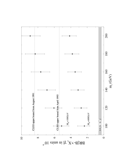
Figure 6: Predictions for $B\rightarrow X_{s}\gamma$ in the 2HDM, as a function of the top-quark mass, with the theoretical uncertainties taken into account (see the text).

For most of the top-quark masses, the results for $M_{H^{\pm}}=100GeV$ in fig. 6 are in contradiction with present measurements, even if the theoretical uncertainties are taken into account. On the other hand, comparing figs. 3 and 6 we can conclude that in the $M_{H^{\pm}}=600GeV$ case we are not able to distinguish between the SM and the 2HDM, independently of the accuracy of future measurements (but assuming the present accuracy of the theoretical predictions).

Figure 7: Lower limits for the charged Higgs boson mass as a function of $\tan\beta$ in the 2HDM (see the text).

Fig. 7 presents the limits in the $tan\beta$-$M_{H^{\pm}}$ plane, obtained by assuming that the excluded values of $tan\beta$ and $M_{H^{\pm}}$ are those for which the inequality (14) holds. The presented limits are found with help of the experimental input from eq. (3). The three solid curves represent lower bounds on $M_{H^{\pm}}$ obtained from $b\rightarrow s\gamma$ for three different values of the top quark mass: 120, 150 and 210 GeV. The dashed curves show bounds coming from the $Z\rightarrow b\bar{b}$ and $b\rightarrow c\tau\bar{\nu}_{\tau}$ decays. The shown $Z\rightarrow b\bar{b}$ bound is based on the results of ref. [27] and corresponds to $m_{t}=150\;GeV$. The $b\rightarrow c\tau\bar{\nu}_{\tau}$ bound is given by the simple formula [28]

$$\tan\beta<0.54\frac{M_{H}}{1GeV}.$$ (18)

The $b\rightarrow c\tau\bar{\nu}_{\tau}$ and $Z\rightarrow b\bar{b}$ bounds are complementary to the $b\rightarrow s\gamma$ bound. All other bounds in the $tan\beta$-$M_{H^{\pm}}$ plane (e.g. the ones coming from $B^{0}$-$\bar{B}^{0}$ mixing and other FCNC processes considered in refs. [29]) are weaker than the combination of the three above-mentioned ones.

Our $b\rightarrow s\gamma$ bounds are much weaker than the ones found in refs. [30, 31], because we have taken into account the uncertainties in the theoretical prediction. If we did not take them into account, our bound for $m_{t}$ = 210 GeV would lie as high as the dotted curve in fig. 7.

As one can see, the $b\rightarrow s\gamma$ bounds in fig. 7 are practically independent of $tan\beta$ for its values larger than 2. From the theoretical standpoint, large values of $tan\beta$ are interesting since $tan\beta\simeq m_{t}/m_{b}$ would naturally explain the large splitting between these two masses without necessity of introducing order-of-magnitude different Yukawa couplings [32]. For these $tan\beta$’s it is convenient to plot the $tan\beta$-independent bounds in the $m_{t}$-$M_{H^{\pm}}$ plane. They are presented in fig. 8.

Figure 8: The $b\rightarrow s\gamma$ lower limits for the charged Higgs boson mass as functions of $m_{t}$ for $\tan\beta=2$. See the text for the description of the curves.

The solid line in this figure shows the lower bound for $M_{H^{\pm}}$ obtained using the requirement described in eq. (14). If we require the theoretical prediction for BR[$B\rightarrow X_{s}\gamma$ ] be only one, not two error bars away from the experimental upper limit, then our lower bound on $M_{H^{\pm}}$ is described by the dashed curve in fig. 8. The dotted line in this figure corresponds to assuming that the theoretical prediction is given by its central value, with no uncertainties whatsoever. We present the three curves in order to demonstrate the relevance of taking the theoretical uncertainties into account.

Our limits are much weaker than found in ref. [30], and they do not exclude the $t\rightarrow H^{+}b$ decay of the top-quark. However, they still have to be considered very strong. For the most interesting values of $tan\beta$ they are still more restrictive than the bounds from the $Z\rightarrow b\bar{b}$ decay [27, 33], as well as the bounds from other FCNC processes [29]. The expected new data on $B\rightarrow X_{s}\gamma$ in the nearest future will further improve the bounds on the 2HDM, but the possible improvement is limited by the theoretical uncertainties. Comparison between figs. 3 and 6 shows that for $M_{H^{\pm}}$ larger than around 600 GeV, the present theoretical inaccuracy does not allow to distinguish the 2HDM and SM predictions.
 
4. The structure of $B\rightarrow X_{s}\gamma$ beyond leading logarithms
 
In this section we describe a complete next-to-leading calculation of $B\rightarrow X_{s}\gamma$ in general terms, and check to what extent the theoretical uncertainties due to the $\mu$-dependence can be reduced after performing such a calculation.

The QCD corrections to the $B\rightarrow X_{s}\gamma$ decay contain large logarithms $ln(M^{2}_{W}/m^{2}_{b})$ which have to be resummed with help of the Renormalization Group Equations (RGE). In order to do this, one introduces an effective hamiltonian built out of operators of dimension higher than 4.

$$H_{eff}=-V_{tb}V^{*}_{ts}\frac{G_{F}}{\sqrt{2}}\sum_{i=1}^{8}Q_{i}(\mu)C_{i}(\mu)\equiv-V_{tb}V^{*}_{ts}\frac{G_{F}}{\sqrt{2}}\vec{Q}^{T}(\mu)\vec{C}(\mu)$$ (19)

where $V_{ij}$ are the elements of the CKM matrix, $Q_{i}(\mu)$ are the relevant operators and $C_{i}(\mu)$ are the corresponding Wilson coefficients. The complete set of operators necessary in the $b\rightarrow s\gamma$ case is the following [3]:

$$\begin{array}[]{cc}Q_{1}=&(\bar{s}_{\alpha}c^{\beta})_{V-A}(\bar{c}_{\beta}b^{\alpha})_{V-A}\vspace{0.2cm}\\ Q_{2}=&(\bar{s}_{\alpha}c^{\alpha})_{V-A}(\bar{c}_{\beta}b^{\beta})_{V-A}\vspace{0.2cm}\\ Q_{3}=&(\bar{s}_{\alpha}b^{\alpha})_{V-A}\sum_{q}(\bar{q}_{\beta}q^{\beta})_{V-A}\vspace{0.2cm}\\ Q_{4}=&(\bar{s}_{\alpha}b^{\beta})_{V-A}\sum_{q}(\bar{q}_{\beta}q^{\alpha})_{V-A}\vspace{0.2cm}\\ Q_{5}=&(\bar{s}_{\alpha}b^{\alpha})_{V-A}\sum_{q}(\bar{q}_{\beta}q^{\beta})_{V+A}\vspace{0.2cm}\\ Q_{6}=&(\bar{s}_{\alpha}b^{\beta})_{V-A}\sum_{q}(\bar{q}_{\beta}q^{\alpha})_{V+A}\vspace{0.2cm}\\ Q_{7}=&\frac{e}{8\pi^{2}}m_{b}\bar{s}_{\alpha}\sigma^{\mu\nu}(1+\gamma_{5})b^{\alpha}F_{\mu\nu}\vspace{0.2cm}\\ Q_{8}=&\frac{g}{8\pi^{2}}m_{b}\bar{s}_{\alpha}\sigma^{\mu\nu}(1+\gamma_{5})(T^{a})^{\alpha}_{\beta}b^{\beta}G_{\mu\nu}^{a}\end{array}$$ (20)

where $(\bar{q}q^{\prime})_{V\pm A}=\bar{q}\gamma_{\mu}(1\pm\gamma_{5})q^{\prime}$ and $\sigma_{\mu\nu}=\frac{i}{2}[\gamma_{\mu},\gamma_{\nu}]$. $Q_{1,2}$ are the current-current operators, $Q_{3-6}$ the QCD penguin operators, and $Q_{7,8}$ the “magnetic penguin” operators. In the latter operators we have neglected the terms proportional to the s-quark mass since they give only a correction of order $m^{2}_{s}/m^{2}_{b}$ to the decay rate.

The inclusion of the couplings in the definition of $Q_{7}$ and $Q_{8}$ allows one to discuss the renormalization group evolution in the full analogy with the case of the usual $\Delta S=1$ or $\Delta B=1$ hamiltonians for nonleptonic decays.

Following [34] we write

$$\vec{C}(\mu)=\hat{U}(\mu,M_{W})\vec{C}(M_{W})$$ (21)

where the renormalization group evolution matrix is given generally by

$$\hat{U}(m_{1},m_{2})=T_{g}exp\int_{g(m_{2})}^{g(m_{1})}dg^{\prime}\frac{\hat{\gamma}^{T}(g^{\prime})}{\beta(g^{\prime})}$$ (22)

with $m_{1}<m_{2}$. Here $T_{g}$ denotes such ordering in the coupling constants that they increase from right to left. Next, $\hat{\gamma}(g)$ is the $8\times 8$ anomalous dimension matrix of the operators $Q_{i}$, and $\beta(g)$ is the usual renormalization group function which governs the evolution of $\alpha_{s}$.

Keeping the first two terms in the expansions for $\gamma(g)$ and $\beta(g)$

$$\hat{\gamma}(g)=\hat{\gamma}^{(0)}\frac{g^{2}}{16\pi^{2}}+\hat{\gamma}^{(1)}\frac{g^{4}}{(16\pi^{2})^{2}}\;\;;\;\;\;\;\;\;\;\;\;\;\;\;\;\;\;\;\;\;\;\;\;\beta(g)=-\beta_{0}\frac{g^{3}}{16\pi^{2}}-\beta_{1}\frac{g^{5}}{(16\pi^{2})^{2}},$$ (23)

where $\beta_{0}=11-\frac{2}{3}f$ and $\beta_{1}=102-\frac{38}{3}f$, one finds [34]:

$$\hat{U}(m_{1},m_{2})=\left(\hat{1}+\frac{\alpha_{s}(m_{1})}{4\pi}\hat{J}\right)\hat{U}^{(0)}(m_{1},m_{2})\left(\hat{1}-\frac{\alpha_{s}(m_{2})}{4\pi}\hat{J}\right)$$ (24)

where $\hat{U}^{(0)}(m_{1},m_{2})$ denotes the evolution matrix in the leading logarithmic approximation and $\hat{J}$ summarizes the next-to-leading corrections to this evolution. If

$$\hat{\gamma}^{(0)}_{D}\equiv\hat{V}^{-1}\hat{\gamma}^{(0)T}\hat{V};\hskip 85.35826pt\hat{G}\equiv\hat{V}^{-1}\hat{\gamma}^{(1)T}\hat{V}$$ (25)

where $\hat{\gamma}^{(0)}_{D}$ denotes a diagonal matrix whose diagonal elements are the components of the vector $\vec{\gamma}^{(0)}$, then

$$\hat{U}^{(0)}(m_{1},m_{2})=\hat{V}\left[\left(\frac{\alpha_{s}(m_{2})}{\alpha_{s}(m_{1})}\right)^{\vec{a}}\right]_{D}\hat{V}^{-1}\hskip 14.22636pt{\rm with}\hskip 14.22636pt\vec{a}=\frac{\vec{\gamma}^{(0)}}{2\beta_{0}}.$$ (26)

For the matrix $\hat{J}$ one gets

$$\hat{J}=\hat{V}\hat{S}\hat{V}^{-1}$$ (27)

where the elements of $\hat{S}$ are given by

$$S_{ij}=\delta_{ij}\gamma_{i}^{(0)}\frac{\beta_{1}}{2\beta_{0}^{2}}-\frac{G_{ij}}{2\beta_{0}+\gamma_{i}^{(0)}-\gamma_{j}^{(0)}}$$ (28)

with $\gamma_{i}^{(0)}$ denoting the elements of $\vec{\gamma}^{(0)}$ and $G_{ij}$ the elements of $\hat{G}$.

The ratio $\alpha_{s}(m_{2})/\alpha_{s}(m_{1})$ in eq. (26) has now to be calculated with help of the two-loop renormalization group equation for $\alpha_{s}(\mu)$. Once $\alpha_{s}(M_{Z})$ is treated as an initial condition for this equation, the corresponding solution takes the form

$$\alpha_{s}(\mu)=\frac{\alpha_{s}(M_{Z})}{v(\mu)}\left[1-\frac{\beta_{1}}{\beta_{0}}\frac{\alpha_{s}(M_{Z})}{4\pi}\frac{ln\;v(\mu)}{v(\mu)}\right]$$ (29)

where $v(\mu)$ is exactly as in eq. (10).

To the same level of accuracy we expand $\vec{C}(M_{W})$ as follows

$$\vec{C}(M_{W})=\vec{C}^{(0)}(M_{W})+\frac{\alpha_{s}(M_{W})}{4\pi}\vec{C}^{(1)}(M_{W}).$$ (30)

The nonvanishing $C^{(0)}_{i}(M_{W})$ have been given in eqs. (7)–(9).

The leading logarithmic approximation to $C_{i}(\mu)$ is completely known. It is obtained by setting $\hat{J}=0$ and $\vec{C}^{(1)}=0$ in eqs. (24) and (30) respectively. In the appendix, we explicitly give the matrix $\hat{\gamma}^{(0)}$ calculated [9] in a certain regularization scheme called the HV scheme. The scheme dependence of $\hat{\gamma}^{(0)}$ will be discussed below. Here we would like only to remark that the $6\times 6$ submatrix of $\hat{\gamma}^{(0)}$ describing mixing of $(Q_{1},Q_{2},...,Q_{6})$ and the $2\times 2$ submatrix for $(Q_{7},Q_{8})$ follow from one-loop calculations. On the other hand, the leading order mixing between these two sectors results from two-loop diagrams.

Let us enumerate what has been already calculated in the literature and which calculations are still required in order to complete the next-to-leading calculation of $C_{i}(\mu)$. Beyond the leading order, $\hat{\gamma}^{(1)}$ and $\vec{C}^{(1)}(M_{W})$ have to be calculated. Actually, the $6\times 6$ submatrix of $\hat{\gamma}^{(1)}$ describing the two-loop mixing of $(Q_{1},...,Q_{6})$ and the corresponding initial conditions in $\vec{C}^{(1)}(M_{W})$ have been already calculated in refs. [34, 35]. The remaining ingredients of a next-to-leading analysis of $\vec{C}(\mu)$ are:
 
(i) The two-loop mixing in the $(Q_{7},Q_{8})$ sector of $\hat{\gamma}^{(1)}$. This calculation is currently being performed [36].
 
(ii) The three-loop mixing between the sectors $(Q_{1},...,Q_{6})$ and $(Q_{7},Q_{8})$ which with our normalizations contribute to $\hat{\gamma}^{(1)}$.
 
(iii) The ${\cal O}(\alpha_{s})$ corrections to $C_{7}(M_{W})$ and $C_{8}(M_{W})$ in eqs. (8) and (9). This requires evaluation of two-loop penguin diagrams with internal W and top quark masses and a proper matching with the effective five-quark theory. An attempt to calculate the necessary two-loop Standard Model diagrams has been recently made in ref. [37]. The effective theory one-loop diagrams with $Q_{7}$ and $Q_{8}$ insertions have been calculated in ref. [24]. However, the finite parts of the effective theory two-loop diagrams with the insertions of the four-quark operators (see figs. 5 and 6 of ref. [7]) are still unknown.
 
All these calculations are very involved, and the necessary three-loop calculation is a truly formidable task! Yet, as will be evident from the following discussion, all these calculations have to be done if we want to reduce the theoretical uncertainties in $b\rightarrow s\gamma$ to around 10%.

It is important to stress that a next-to-leading calculation performed without resumming large logarithms $ln(M^{2}_{W}/m^{2}_{b})$ would not be more accurate than the present leading-order one where these logarithms are resummed. This is why the calculation of the three-loop mixing is unavoidable.
 
Once the evolution of the coefficients $C_{i}(\mu)$ down to the scale $\mu\sim m_{b}$ is performed, one has to evaluate the matrix elements of all the operators at this scale.

In the leading order, only the tree-level matrix element of $Q_{7}$ and the one-loop matrix elements of $Q_{1}-Q_{6}$ that are of order $\alpha_{s}^{0}$ have to be included. The latter matrix elements vanish for the on-shell photon in any 4-dimensional regularization scheme and also in the HV scheme, i.e. dimensional regularization with the ’t Hooft-Veltman definition of $\gamma_{5}$ [38]. All but the last [9] calculations of the leading order QCD corrections to $b\rightarrow s\gamma$ used the NDR scheme, i.e. the dimensional regularization with fully anticommuting $\gamma_{5}$. In this scheme, the one-loop $b\rightarrow s\gamma$ matrix elements of some of the four-quark operators $Q_{1},...,Q_{6}$ do not vanish for the on-shell photon but are proportional to the tree-level matrix element of $Q_{7}$ (even for the quarks off-shell).

The regularization scheme-dependence of leading order matrix elements is a peculiar feature of the $b\rightarrow s\gamma$ decay. It can arise because one-loop mixing between the $(Q_{1},...,Q_{6})$ and $(Q_{7},Q_{8})$ sectors vanishes. In consequence, what usually would be a next-to-leading order effect is only a leading one. And what would usually be next-next-to-leading (like the above-mentioned three-loop mixing) is only next-to-leading.

This peculiarity causes, that at the leading order it is convenient to introduce the so-called “effective coefficients” for the operators $Q_{7}$ and $Q_{8}$: First, we observe that in any regularization scheme one can write the one-loop matrix elements of the four-quark operators $Q_{1},...,Q_{6}$ as

$$\langle Q_{i}{}\rangle_{\scriptscriptstyle one\;\;loop}=y_{i}\langle Q_{7}\rangle_{\scriptscriptstyle tree},\hskip 28.45274pti=1,...,6$$ (31)

for the on-shell photon but quarks possibly off-shell. In consequence, the leading order $b\rightarrow s\gamma$ matrix element of $H_{eff}$ is equal to the tree level matrix element of

$$-V_{tb}V^{*}_{ts}\frac{G_{F}}{\sqrt{2}}C^{(0)eff}_{7}(\mu)O_{7}$$ (32)

where

$$C^{(0)eff}_{7}(\mu)=C^{(0)}_{7}(\mu)+\sum_{i=1}^{6}y_{i}C^{(0)}_{i}(\mu).$$ (33)

In the HV scheme all the $y_{i}$’s vanish, while in the NDR scheme $\vec{y}=(0,0,0,0,-\frac{1}{3},-1)$. This regularization scheme dependence is cancelled by a corresponding regularization scheme dependence in $\hat{\gamma}^{(0)}$ (see ref. [9] for details). Consequently, the quantity $C^{(0)eff}_{7}(\mu)$ defined in eq. (33) and used in eq. (4) is scheme-independent.

The numbers $y_{i}$ in eq. (31) come from divergent, i.e. purely short-distance parts of the one-loop integrals. So no reference to the spectator-model is necessary here. This is why one is allowed to treat the expression (32) as the proper effective hamiltonian that has to be inserted in between hadronic states in a calculation of, say, the $B\rightarrow K^{*}\gamma$ decay.

An “effective coefficient” for the operator $Q_{8}$ introduced in a similar way equals to

$$C^{(0)eff}_{8}(\mu)=C^{(0)}_{8}(\mu)+\sum_{i=1}^{6}z_{i}C^{(0)}_{i}(\mu)$$ (34)

where the numbers $z_{i}$ are defined by the one-loop $b\rightarrow s\;gluon$ on-shell matrix elements of the four-quark operators:

$$\langle Q_{i}\rangle_{\scriptscriptstyle one\;\;loop}=z_{i}\langle Q_{8}\rangle_{\scriptscriptstyle tree},\hskip 28.45274pti=1,...,6.$$ (35)

All the $z_{i}$’s vanish in the HV scheme, while in the NDR scheme we have $\vec{z}=(0,0,0,0,1,0)$.

For later convenience we introduce a scheme-independent vector

$$\vec{C}^{(0)eff}(\mu)=\left[C^{(0)}_{1}(\mu),....,C^{(0)}_{6}(\mu),C^{(0)eff}_{7}(\mu),C^{(0)eff}_{8}(\mu)\right].$$ (36)

From the RGE for $\vec{C}^{(0)}(\mu)$ it is straighforward to derive the RGE for $\vec{C}^{(0)eff}(\mu)$. It has the form

$$\mu\frac{d}{d\mu}C^{(0)eff}_{i}(\mu)=\gamma^{(0)eff}_{ji}C^{(0)eff}_{j}(\mu)$$ (37)

where

$$\gamma^{(0)eff}_{ji}=\left\{\begin{array}[]{cc}\gamma^{(0)}_{j7}+\sum_{k=1}^{6}y_{k}\gamma^{(0)}_{jk}-y_{j}\gamma^{(0)}_{77}-z_{j}\gamma^{(0)}_{87}&\mbox{when $i=7$ and $j=1,...,6$}\\ \gamma^{(0)}_{j8}+\sum_{k=1}^{6}z_{k}\gamma^{(0)}_{jk}-z_{j}\gamma^{(0)}_{88}&\mbox{when $i=8$ and $j=1,...,6$}\\ \gamma^{(0)}_{ji}&\mbox{otherwise.}\end{array}\right.$$ (38)

The matrix $\hat{\gamma}^{(0)eff}$ is a scheme-independent quantity. We give it explicitly in the appendix.

At the next-to-leading level the situation is not as simple. One has then to include one-loop $b\rightarrow s\gamma$ matrix elements of $Q_{7}$ and $Q_{8}$, and two-loop matrix elements of $Q_{1},...,Q_{6}$. As long as the photon and the external quarks are put on-shell, we can still formally write the considered matrix elements as proportional to the tree-level matrix element of $Q_{7}$. One could naively expect that the proportionality constants depend only on the ratio $\mu/m_{b}$ because after neglection of the s-quark mass, we have only a single scale in the process. Unfortunately, they also depend on the infrared regulator used in the calculation. However, their $\mu$-dependence is still a purely short-distance effect and can be found with help of the existing leading-order results.

As discussed in ref. [40], the $\mu$-dependence of $\langle\vec{Q}(\mu)\rangle$ can be calculated in a renormalization group improved perturbation theory, as long as $\mu$ is not too small. Taking the scale $m_{b}$ as a reference point, the $\mu$-dependence of $\langle\vec{Q}(\mu)\rangle$ is simply given by

$$\langle\vec{Q}^{T}(\mu)\rangle=\langle\vec{Q}^{T}(m_{b})\rangle\hat{U}(m_{b},\mu)$$ (39)

with $\hat{U}$ given already in eq. (24). The scale $m_{b}$ is chosen here only for convenience. Inserting eqs. (21) and (39) into the final expression for the $b\rightarrow s\gamma$ amplitude:

$$A(b\rightarrow s\gamma)=-V_{tb}V^{*}_{ts}\frac{G_{F}}{\sqrt{2}}\sum_{i=1}^{8}\langle Q_{i}(\mu)\rangle C_{i}(\mu)$$ (40)

one finds that the $\mu$-dependence present in $\vec{C}(\mu)$ is cancelled by the corresponding $\mu$-dependence in $\langle\vec{Q}(\mu)\rangle$.

Let us now write the sum of the tree and one-loop on-shell matrix elements of $Q_{7}$ and $Q_{8}$ calculated at $\mu=m_{b}$ as

$$\langle Q_{i}(m_{b})\rangle=\left[\delta_{i7}+\frac{\alpha_{s}(m_{b})}{4\pi}r_{i7}\right]\langle Q_{7}(m_{b})\rangle_{tree},\;\;\;\;\;\;\;i=7,8,$$ (41)

and the sum of one- and two-loop on-shell matrix elements of $Q_{1},...,Q_{6}$ as

$$\langle Q_{i}(m_{b})\rangle=\left[y_{i}+\frac{\alpha_{s}(m_{b})}{4\pi}r_{i7}\right]\langle Q_{7}(m_{b})\rangle_{tree},\;\;\;\;\;\;\;i=1,...,6.$$ (42)

As long as the infrared divergencies are regulated dimensionally, the $r_{i7}$’s do not contain dimensionful parameters, i.e. they are either pure numbers or depend only on the infrared regulator $\epsilon_{\scriptscriptstyle IR}$.

If $\mu\sim m_{b}$, there are no large logarithms present in $\langle\vec{Q}(\mu)\rangle$, and the resummation of logarithms is not needed in eq. (39). Therefore expanding eq. (39) around $\mu=m_{b}$ we can reproduce the $\mu$-dependent terms that would appear in the straightforward perturbative calculation of $\langle\vec{Q}(\mu)\rangle$. Using eqs. (39)–(42) and expanding the matrix $\hat{U}(m_{b},\mu)$ from eq. (39) around $\mu=m_{b}$ we find, that the $b\rightarrow s\gamma$ amplitude calculated in terms of the coefficients renormalized at any scale $\mu\sim m_{b}$ can be written in the following form:

$$A(b\rightarrow s\gamma)=-V_{tb}V^{*}_{ts}\frac{G_{F}}{\sqrt{2}}\;\;D\;\;\langle Q_{7}(m_{b})\rangle_{tree}$$ (43)

where

$$D=C_{7}^{eff}(\mu)+\frac{\alpha_{s}(m_{b})}{4\pi}\left(C_{i}^{(0)eff}(\mu)\gamma^{(0)eff}_{i7}ln\frac{m_{b}}{\mu}+C_{i}^{(0)}(\mu)r_{i7}\right).$$ (44)

All the $C_{i}$’s in the expression (33) for $C_{7}^{eff}(\mu)$ are now taken up to next-to-leading accuracy. The term proportional to $ln\frac{m_{b}}{\mu}$ comes solely from expanding $\langle\vec{Q}(\mu)\rangle$ around $\mu=m_{b}$. The tree-level matrix element of $Q_{7}$ is denoted as $\langle Q_{7}(m_{b})\rangle_{tree}$ in order to point out that the mass $m_{b}$ in the normalization of this operator is renormalized at the scale $\mu=m_{b}$.

A next-to-leading generalization of eq. (4) takes the following form:

$$R=\frac{\Gamma[b\rightarrow s\gamma]}{\Gamma[b\rightarrow ce\bar{\nu}_{e}]}=\frac{|V_{ts}^{*}V_{tb}|^{2}}{|V_{cb}|^{2}}\frac{6\alpha_{\scriptscriptstyle QED}}{\pi g(z)}F|D|^{2}.$$ (45)

with D defined in eq. (44), and the factor F given by

$$F=\left(\frac{m_{b}(\mu=m_{b})}{m_{b}^{pole}}\right)^{2}\frac{1}{\kappa(z)}.$$ (46)

The quantity $\kappa(z)$ is a sizable next-to-leading QCD correction to the semileptonic decay [41]

$$\kappa(z)\simeq 1-\frac{2\alpha_{s}(m_{b})}{3\pi}\left[(\pi^{2}-\frac{31}{4})(1-z)^{2}+\frac{3}{2}\right].$$ (47)

which tends to cancel with the other factor in eq. (46)

$$\left(\frac{m_{b}(\mu=m_{b})}{m_{b}^{pole}}\right)^{2}=1-\frac{8}{3}\frac{\alpha_{s}(m_{b})}{\pi},$$ (48)

and, in consequence, the expression (46) differs from unity by only around 8%.

The origin of the latter factor is very simple: We have normalized the $b\rightarrow s\gamma$ rate to the semileptonic rate in order to cancel factors $m_{b}^{5}$ in front of the spectator-model expressions. However, in the semileptonic case, all five factors of $m_{b}$ come from the on-shell external lines, while in the case of $b\rightarrow s\gamma$ two of the $m_{b}$’s come from the normalization of $Q_{7}$, and should be taken in the same renormalization scheme as the coefficients. This becomes even more obvious when one realizes that the anomalous dimension matrix element $\gamma^{(0)}_{77}=\frac{32}{3}$ is dominated by the anomalous dimension $\gamma^{(0)}_{m}=\frac{24}{3}=8$ of the mass $m_{b}$ which normalizes $Q_{7}$. If we did not include the running $m_{b}(\mu)$ in the operator normalization, then our coefficients would run differently than described in eq. (5).

Let us now return to the complete next-to-leading expressions (43)–(44) for the $b\rightarrow s\gamma$ amplitude. From eq. (44) and from the RGE (37) for $\vec{C}^{(0)eff}(\mu)$ one can easily see that the dominant $\mu$-dependence in the leading logarithmic coefficient $C^{(0)eff}_{7}(\mu)$ will be cancelled by the logarithms coming from the next-to-leading matrix elements. Consequently, the resulting $\mu$-dependence of the obtained result will be one order higher than the accuracy of the performed calculation, as it always must happen in any perturbative calculation.

We can explicitly check the cancellation of $\mu$-dependence, because the coefficients at the logarithms in eq. (44) are given by the matrix $\hat{\gamma}^{(0)eff}$ which is already known (see the appendix). However, any change of $\mu$ is equivalent to a shift in the unknown constant terms $r_{i7}$. Consequently, a meaningful analysis of the $\mu$-dependence must also include $r_{i7}$. These constants are generally renormalization-scheme dependent, and this dependence can only be cancelled by calculating $\hat{\gamma}^{(1)}$ in the same renormalization scheme. Since this point has been extensively discussed in several papers [34, 35, 40], we will not repeat this discussion here. However, it is clear from these remarks, that in order to address the $\mu$-dependence and the renormalization-scheme dependence as well as their cancellations, it is necessary to perform a complete next-to-leading order analysis of $\vec{C}(\mu)$ along the lines presented above, and to calculate the constants $r_{i7}$ in eqs. (41) and (42).

The program of calculating the complete next-to-leading contributions and reducing the $\mu$-dependence has been already accomplished in several other weak decays. In ref. [12] the $\mu$-dependence in top-quark contributions to $K^{0}$-$\bar{K}^{0}$ and $B^{0}$-$\bar{B}^{0}$ mixings have been considered. A similar analysis of the charm quark contribution to $K^{0}$-$\bar{K}^{0}$ mixing has been recently done in ref. [13]. Next, in ref. [14] the $\mu$-dependences in rare decays $K_{L}\rightarrow\pi^{0}\nu\bar{\nu}$, $K^{+}\rightarrow\pi^{+}\nu\bar{\nu}$, $K_{L}\rightarrow\mu\bar{\mu}$, $B\rightarrow l\bar{l}$ and $B\rightarrow X_{s}\nu\bar{\nu}$ have been studied. In all these papers it has been demonstrated explicitly that the inclusion of next-to-leading corrections considerably reduced the $\mu$-dependence present in the leading order expressions. The remaining $\mu$-dependence can be further reduced only by including still higher order terms in the renormalization group improved perturbation theory.

In view of the tremendous complexity of the next-to-leading calculations for $b\rightarrow s\gamma$, we are not yet in a position to make a similar analysis for this decay. We can however perform a simple exercise with the terms we already know, in order to get a rough idea by how much a future next-to-leading order calculation could reduce the $\mu$-dependence shown by the solid line in fig. 2.

We proceed as follows: We set $\hat{J}=0$ and $\vec{C}^{(1)}=0$ in eqs. (24) and (30) respectively, i.e. we calculate $\vec{C}^{eff}(\mu)$ in the leading logarithmic approximation. $C^{(0)eff}_{7}(\mu)$ has been already given in eq. (5). For the remaining coefficients we find

$$\begin{array}[]{ccc}\vspace{0.2cm}C^{(0)}_{1}(\mu)=&-\frac{1}{2}\eta^{-\frac{12}{23}}+\frac{1}{2}\eta^{\frac{6}{23}}&\\ \vspace{0.2cm}C^{(0)}_{2}(\mu)=&\frac{1}{2}\eta^{-\frac{12}{23}}+\frac{1}{2}\eta^{\frac{6}{23}}&\\ \vspace{0.2cm}C^{(0)}_{3}(\mu)=&\frac{1}{6}\eta^{-\frac{12}{23}}-\frac{1}{14}\eta^{\frac{6}{23}}&+0.0510\eta^{0.4086}-0.1403\eta^{-0.4230}-0.0113\eta^{-0.8994}+0.0054\eta^{0.1456}\\ \vspace{0.2cm}C^{(0)}_{4}(\mu)=&-\frac{1}{6}\eta^{-\frac{12}{23}}-\frac{1}{14}\eta^{\frac{6}{23}}&+0.0984\eta^{0.4086}+0.1214\eta^{-0.4230}+0.0156\eta^{-0.8994}+0.0026\eta^{0.1456}\\ \vspace{0.2cm}C^{(0)}_{5}(\mu)=&&-0.0397\eta^{0.4086}+0.0117\eta^{-0.4230}-0.0025\eta^{-0.8994}+0.0304\eta^{0.1456}\\ \vspace{0.2cm}C^{(0)}_{6}(\mu)=&&0.0335\eta^{0.4086}+0.0239\eta^{-0.4230}-0.0462\eta^{-0.8994}-0.0112\eta^{0.1456}\end{array}$$ (55)

and

$$C^{(0)eff}_{8}(\mu)=(C^{(0)}_{8}(M_{W})+\frac{313063}{363036})\eta^{\frac{14}{23}}-\hskip 284.52756pt$$

$$\hskip 128.0374pt-0.9135\eta^{0.4086}+0.0873\eta^{-0.4230}-0.0571\eta^{-0.8994}-0.0209\eta^{0.1456}$$

Next, we set $r_{i7}=0$ in eq. (43), except for $r_{27}$ for which we consider values $-2$, $0$ and $2$. It is clear from eqs. (41)–(42) that all the $r_{i7}$’s can take values of order 1. We choose to vary $r_{27}$ because it is the operator $Q_{2}$ that has the largest coefficient — the coefficient $C_{2}^{(0)}(m_{b})$ is around 1.1. The “next-to-leading” results for the ratio R found this way are presented as functions of $\mu$ by the dashed lines in fig. 2.

One can see that the $\mu$-dependence is much weaker than for the leading-order results (the solid line), but not completely absent. The initial $\pm 25\%$ uncertainty is reduced to around $\pm 3\%$. The dominant $\mu$-dependence caused by factors of order $\alpha_{s}(m_{b})ln(m_{b}/\mu)$ cancels out, but we still have noncancelling higher order terms like $\alpha_{s}^{2}(m_{b})ln^{2}(m_{b}/\mu)$ or $\alpha_{s}^{2}(m_{b})ln(m_{b}/\mu)$. We have organized our exercise in such a way that both kinds of the latter terms do appear, in spite of that we have set a lot of the next-to-leading corrections to zero. The higher order $\mu$-dependence could be, in principle, removed by including still higher order QCD corrections.

Now it is easy to see that, indeed, a reasonable variation in possible non-logarithmic next-to-leading terms, namely changing $r_{27}$ from $-2$ to $2$, causes a similar change in the final results as varying $\mu$ by a factor of 2 in the leading order terms. This supports the method we have used for estimating the size of the NLL corrections in our phenomenological discussion in section 3.

The simple exercise presented above explicitly illustrates the cancellation of the $\mu$-depen- dence present in the leading-order expressions. It cannot, however, replace the full next-to-leading order calculation. Indeed, we still do not know which of the dashed curves in fig. 2 is closest to the true next-to-leading result. Our exercise is, nevertheless, rather encouraging as it shows that the theoretical prediction for $B\rightarrow X_{s}\gamma$ will be considerably improved once all the next-to-leading calculations are completed.
 
5. Conclusions
 
i) Among many theoretical uncertainties present in the calculation of the $B\rightarrow X_{s}\gamma$ decay, the most important one is due to the absence of a complete calculation of next-to-leading short-distance QCD corrections to this decay. It causes around $\pm 25\%$ inaccuracy in the prediction for this decay rate, while all the other uncertainties are around or below 10%.

ii) Once the present experimental data are taken into account, it is quite improbable that a future precise measurement of the $B\rightarrow X_{s}\gamma$ rate will contradict the Standard Model prediction, in view of its large uncertainty. However, if the future measurement of the inclusive rate is close to the present upper bound, then some useful correlation between $m_{t}$ and $\alpha_{s}(M_{Z})$ will emerge.

iii) In spite of the theoretical uncertainties, the present experimental data still put quite strong bounds on the parameters of the Two-Higgs-Doublet Model. The $b\rightarrow s\gamma$, $Z\rightarrow b\bar{b}$ and $b\rightarrow c\tau\bar{\nu}_{\tau}$ processes are enough to give the most stringent bounds in the $M_{H^{\pm}}$-$tan\beta$ plane. However, our $b\rightarrow s\gamma$ bounds are weaker than found by other authors.

iv) The theoretical prediction can be significantly improved by making a systematic next-to-leading calculation within the framework of renormalization group improved perturbation theory. Such a calculation is very involved, since it requires a calculation of finite parts of many two-loop diagrams, and divergent parts of three-loop diagrams. However, it has to be done if we want to make the uncertainty coming from short-distance effects smaller than the other uncertainties.

v) The uncertainty in the leading order prediction is best signaled by its strong dependence on the renormalization scale $\mu$ at which the RGE evolution is terminated. We have described in detail how this dependence is reduced in a full next-to-leading result, and performed a simple exercise to check it numerically. As a result, we can conclude that once a next-to-leading result is found, its $\mu$-dependence should be below 5%, for $\mu$ changing from $m_{b}/2$ to $2m_{b}$.

Acknowledgements

We would like to thank the authors of refs. [27, 33] for sending their results to us prior to publication.

6. Appendix
 
Here we give the scheme-independent matrix $\hat{\gamma}^{(0)eff}$ defined in eq. (38) that governs the leading-logarithmic QCD corrections to $b\rightarrow s\gamma$ . In the HV scheme this matrix is equal to the matrix $\hat{\gamma}^{(0)}$ of eq. (23).

$$\hat{\gamma}^{(0)eff}=\left[\begin{array}[]{cccccccc}\vspace{0.2cm}-2&6&0&0&0&0&0&3\\ \vspace{0.2cm}6&-2&-\frac{2}{9}&\frac{2}{3}&-\frac{2}{9}&\frac{2}{3}&\frac{416}{81}&\frac{70}{27}\\ \vspace{0.2cm}0&0&-\frac{22}{9}&\frac{22}{3}&-\frac{4}{9}&\frac{4}{3}&-\frac{464}{81}&\frac{140}{27}+3f\\ \vspace{0.2cm}0&0&6-\frac{2}{9}f&-2+\frac{2}{3}f&-\frac{2}{9}f&\frac{2}{3}f&\frac{416}{81}u-\frac{232}{81}d&6+\frac{70}{27}f\\ \vspace{0.2cm}0&0&0&0&2&-6&\frac{32}{9}&-\frac{14}{3}-3f\\ \vspace{0.2cm}0&0&-\frac{2}{9}f&\frac{2}{3}f&-\frac{2}{9}f&-16+\frac{2}{3}f&-\frac{448}{81}u+\frac{200}{81}d&-4-\frac{119}{27}f\\ \vspace{0.2cm}0&0&0&0&0&0&\frac{32}{3}&0\\ \vspace{0.2cm}0&0&0&0&0&0&-\frac{32}{9}&\frac{28}{3}\\ \end{array}\right]$$

where f = u + d, and u (d) is the number of up- (down-) quarks in the effective theory. In our case $u=2$ and $d=3$.

The above matrix has been obtained under the assumption that the disagreements between refs. [7], [8] and [9] concerning $\gamma^{(0)}_{57}$, $\gamma^{(0)}_{58}$ and $\gamma^{(0)}_{68}$ in the NDR scheme are resolved in favour of ref. [9]. More information about these disagreements is contained in the appendix of ref. [39]. Here we only mention that these disagreements make the numerical leading order results differ by only around 1%, so they are irrelevant for our phenomenological discussion. Note, that our normalization of $Q_{7}$ and $Q_{8}$ differs from the one used in ref. [9].

The scheme-independent numbers $a_{i}$ and $h_{i}$ in eq. (5) are given by the eigenvalues and eigenvectors of $\hat{\gamma}^{(0)eff}$ . Their explicit values are given by

$$\begin{array}[]{ccccccccc}\vspace{0.2cm}a_{i}=(&\frac{14}{23},&\frac{16}{23},&\frac{6}{23},&-\frac{12}{23},&0.4086,&-0.4230,&-0.8994,&0.1456)\\ h_{i}=(&\frac{626126}{272277},&-\frac{56281}{51730},&-\frac{3}{7},&-\frac{1}{14},&-0.6494,&-0.0380,&-0.0186,&-0.0057)\end{array}$$ (56)

With help of Mathematica [42], all the above numbers can be found exactly. However, some of them are so complicated that it is much better to keep them numerically.

References

-
[1]
E. Golowich and S. Pakvasa, Phys. Lett. B205 (1988) 393;
M. R. Ahmady, D. Liu and Z. Tao, preprint IC/93/26 (hep-ph 9302209) -
[2]
S. Bertolini, F. Borzumati and A. Masiero,
Phys. Rev. Lett. 59 (1987) 180;
N. G. Deshpande, P. Lo, J. Trampetic, G. Eilam and P. Singer, Phys. Rev. Lett. 59 (1987) 183 - [3] B. Grinstein, R. Springer and M.B. Wise, Nucl. Phys. B339 (1990) 269
- [4] R. Grigjanis, P.J. O’Donnell, M. Sutherland and H. Navelet, Phys. Lett. B213 (1988) 355, Phys. Lett. B286 (1992) 413E
- [5] G. Cella, G. Curci, G. Ricciardi and A. Vicere, Phys. Lett. B248 (1990) 181
- [6] M. Misiak, Phys. Lett. B269 (1991) 161
- [7] M. Misiak, Nucl. Phys. B393 (1993) 23
- [8] K. Adel and Y.P. Yao, Modern Physics Letters A8 (1993) 1679
- [9] M. Ciuchini, E. Franco, G. Martinelli, L. Reina and L. Silvestrini, Phys. Lett. B316 (1993) 127
- [10] R. Ammar et. al., Phys. Rev. Lett. 71 (1993) 674
- [11] A. Ali, C. Greub and T. Mannel, “Rare decays in the Standard Model”, in Proc. ECFA Workshop on B-Meson Factory, eds. R. Aleksan and A. Ali, DESY, March 1993.
- [12] A. J. Buras, M. Jamin and P .H. Weisz, Nucl. Phys. B347 (1990) 491
- [13] S. Herrlich and U. Nierste, preprint TUM-T31-49/93 (hep-ph 9310311)
- [14] G. Buchalla and A. J. Buras, Nucl. Phys. B398 (1993) 285, Nucl. Phys. B400 (1993) 225, preprint TUM-T31-44/93 (hep-ph 9308272)
- [15] T. Inami and C. S. Lim, Prog. Theor. Phys. 65 (1981) 297, 65 (1981) 1772E
- [16] P. Cho and M. Misiak, preprint CALT-68-1893 (hep-ph 9310332)
-
[17]
S. Bertolini, F. Borzumati, A. Masiero and G. Ridolfi,
Nucl. Phys. B353 (1991) 591;
F. Borzumati, preprint DESY 93-090 (hep-ph 9310212) -
[18]
J. Chay, H. Georgi and B. Grinstein, Phys. Lett. B247 (1990) 399;
J. D. Bjorken, I. Dunietz and J. Taron, Nucl. Phys. B371 (1992) 111;
I. I. Bigi, B. Blok, M. Shifman, N. G. Uraltsev and A. I. Vainshtein, preprint NFF-ITP-92-156 (hep-ph 9212227), published in DPF conference proceedings (1992) p.610 - [19] R. Rückl, preprint MPI-Ph/36/89
- [20] V. Lüth, talk at Lepton-Photon Symposium, Cornell, August 1993.
- [21] see e.g. P. Langacker and N. Polonsky, Phys. Rev. D47 (1993) 4028
- [22] Review of Particle Properties, Phys. Rev. D45 (1992) No. 11, part II
- [23] P. Cho, B. Grinstein, Nucl. Phys. B365 (1991) 279
- [24] A. Ali and C. Greub, Phys. Lett. B259 (1991) 182
-
[25]
P. Ball, preprint TUM-T31-43/93, hep-ph 9308244;
P. Colangelo, C. A. Dominguez, G. Nardulli and N. Paver, preprint BARI-TH/93-150 (hep-ph 9308264);
A. Ali, T. Ohl and T. Mannel, Phys. Lett. B298 (1993) 195;
A. Ali and C. Greub, preprint ZU-TH 11/93;
P. J. O’Donnell and H. K. K. Tung, Phys. Rev. D48 (1993) 2145;
B. Holdom and M. Sutherland, preprint UTPT-93-22 (hep-ph 9308313);
T. Hayashi, M. Matsuda, M. Tanimoto, preprint AUE-01-93 - [26] L. F. Abott, P. Sikivie and M. B. Wise, Phys. Rev. D21 (1980) 1393
- [27] F. Cornet, W. Hollik, W. Mösle, to be published
-
[28]
P. Krawczyk and S. Pokorski, Phys. Rev. Lett. 60 (1988) 182;
G. Isidori, Phys. Lett. B298 (1993) 409 -
[29]
A. J. Buras, P. Krawczyk, M. E. Lautenbacher and
C. Salazar, Nucl. Phys. B337 (1990) 284;
J. Gunion and B. Grza̧dkowski, Phys. Lett. B243 (1990) 301 - [30] J. L. Hewett, Phys. Rev. Lett. 70 (1993) 1045
- [31] V. Barger, M. S. Berger and R. J. N. Phillips, Phys. Rev. Lett. 70 (1993) 1368
-
[32]
G. C. Branco, A. J. Buras, J. M. Gerard, Nucl. Phys. B259 (1985) 306;
S. Pokorski, “How is the isotopic spin symmetry of quark masses broken?”, in Proc. XII th Int. Workshop on Weak Interactions and Neutrinos, Ginosar, Israel, April 1989. - [33] G. Park, preprint CTP-TAMU-69/93 (hep-ph 9311207)
- [34] A. J. Buras, M. Jamin, M. E. Lautenbacher and P .H. Weisz, Nucl. Phys. B370 (1992) 69, Nucl. Phys. B400 (1993) 37
-
[35]
G. Altarelli, G. Curci, G. Martinelli and
S. Petrarca, Nucl. Phys. B187 (1981) 461;
A. J. Buras and P .H. Weisz, Nucl. Phys. B333 (1990) 66;
M. Ciuchini, E. Franco, G. Martinelli and L. Reina, preprint ROME 92/913 (hep-ph 9304257) - [36] M. Misiak and M. Münz, in preparation
- [37] K. Adel and Y.P. Yao, preprint UM-TH-93-20 (hep-ph 9308349)
-
[38]
G. ’t Hooft and M. Veltman, Nucl. Phys. B44 (1972) 189;
P. Breitenlohner and D. Maison, Commun. Math. Phys. 52 (1977) 11, 39, 55 - [39] M. Misiak, preprint TUM-T31-46/93 (hep-ph 9309236)
- [40] A. J. Buras, M. Jamin and M. E. Lautenbacher, Nucl. Phys. B408 (1993) 209
-
[41]
N. Cabibbo and L. Maiani, Phys. Lett B79 (1979) 109;
C. S. Kim and A. D. Martin, Phys. Lett. B225 (1989) 186 - [42] S. Wolfram, Mathematica, Addison-Wessley Publ. Comp., N.Y. 1988.