OKHEP-93-08
FINITE-ELEMENT QUANTUM ELECTRODYNAMICS

Abstract

We apply the finite-element lattice equations of motion for quantum electrodynamics to an examination of anomalies in the current operators. By taking explicit lattice divergences of the vector and axial-vector currents we compute the vector and axial-vector anomalies in two and four dimensions. We examine anomalous commutators of the currents to compute divergent and finite Schwinger terms. And, using free lattice propagators, we compute the vacuum polarization in two dimensions and hence the anomaly in the Schwinger model.

This paper summarizes the status of the finite-element approach to gauge theories, in which the Heisenberg operator equations of motion are converted to operator difference equations consistent with unitarity. A review of the entire program, from quantum mechanics to quantum field theory, is given in Ref. [1].

Lattice Propagators We begin by reminding the reader of the form of the free finite-element lattice Dirac equation:

$${i\gamma^{0}\over h}(\psi_{\overline{{\bf m}},n+1} - \psi_{\overline{{\bf m}},n})+{i\gamma^{j}\over\Delta}(\psi_{m_{j}+1,\overline{{\bf m}}_{\perp},\overline{n}}$$ (1)

$$- \psi_{m_{j},\overline{{\bf m}}_{\perp},\overline{n}})-\mu\psi_{\overline{{\bf m}},\overline{n}}=0.$$

Here $\mu$ is the electron mass, $h$ is the temporal lattice spacing, $\Delta$ is the spatial lattice spacing, $\bf m$ represents a spatial lattice coordinate, $n$ a temporal coordinate, and overbars signify forward averaging:

$$x_{\overline{m}}={1\over 2}(x_{m+1}+x_{m}).$$ (2)

It is a straightforward exercise to show that, apart from a contact term, the free electron Green’s function may be expressed as

$$G_{{\bf m},n;{\bf m}^{\prime},n^{\prime}}={h\over 4\pi}\int_{-\pi/h}^{\pi/h}d\hat{\Omega}e^{-ih\hat{\Omega}(n-n^{\prime})}$$

$$\quad\times{1\over L^{3}}\sum_{\bf p}e^{i{\bf p\cdot(m-m^{\prime})}2\pi/M}$$

$$\quad\times{\gamma^{0}\sin h\hat{\Omega}+(\mu-\mbox{\boldmath$\gamma$}\cdot\tilde{\bf p})h\cos^{2}h\hat{\Omega}/2\over\cos h(\Omega-i\epsilon)-\cos h\hat{\Omega}}.$$ (3)

Here the lattice momentum is given by

$$\tilde{\bf p}={2{\bf t}\over\Delta},\quad\tilde{\omega}=\tilde{p}^{0}=\sqrt{\tilde{\bf p}^{2}+\mu^{2}},\quad({{\bf t_{p}}})_{i}=\tan p_{i}\pi/M.$$ (4)

The quantity $\Omega$ is related to $\tilde{\omega}$ by

$$\tilde{\omega}={2\over h}\tan{h\Omega\over 2}.$$ (5)

We take $M$, the number of lattice points in a given spatial direction, to be odd, so that $\psi$ is periodic on the spatial lattice.

A similar expression can be derived for the free photon propagator.

This propagator (3) has been used to perform a calculation of the vacuum polarization in two-dimensional QED, with a result consistent with the anomaly in the Schwinger model, $e^{2}/\pi$. Some typical results are shown in Fig. 1.

Figure 1: Plot of the lattice vacuum polarization $\Pi(0)/(e^{2}/\pi)$ for $M=2533$ as a function of $\nu=\mu\Delta/2$. Shown are curves with $r=h/\Delta=0.1$, 0.75, 0.99.

A similar calculation of the anomaly in four-dimensional electrodynamics is in progress.

Interactions

Interactions of an electron with a background electromagnetic field is given in terms of a transfer matrix $T$:

$$\psi_{n+1}=T_{n}\psi_{n},$$ (6)

which is to be understood as a matrix equation in $\overline{\bf m}$. Explicitly, in the gauge $A^{0}=0$,

$$T=2U^{-1}-1,\quad U=1-{ih\mu\gamma^{0}\over 2}+{h\over\Delta}\gamma^{0}\mbox{\boldmath$\gamma$}\cdot\mbox{\boldmath${\cal D}$},$$ (7)

where

$${\cal D}^{j}_{{\bf m,m^{\prime}}} = (-1)^{m_{j}+m_{j}^{\prime}}[\epsilon_{m_{j},m_{j}^{\prime}}\cos\hat{\zeta}_{m_{j},m^{\prime}_{j}}$$ (8)

$$+ i\sin\hat{\zeta}_{m_{j},m^{\prime}_{j}}]\sec\zeta^{(j)}\,\delta_{{\bf m_{\perp},m^{\prime}_{\perp}}}.$$

Here

$$\epsilon_{m,m^{\prime}}=\left\{\begin{array}[]{ll}1,&m^{\prime}>m,\\ 0,&m^{\prime}=m,\\ -1,&m^{\prime}<m,\end{array}\right.$$ (9)

and (the following are local and unaveraged in ${\bf m}_{\perp}$, $n$)

$$\zeta_{m_{j}}={e\Delta\over 2}A^{j}_{\overline{m_{j}-1}},\quad\zeta^{(j)}=\sum_{m_{j}=1}^{M}\zeta_{m_{j}},$$ (10)

and

$$\hat{\zeta}_{m_{j},m_{j}^{\prime}}=\sum_{m_{j}^{\prime\prime}=1}^{M}{\rm sgn}\,(m_{j}^{\prime\prime}-m_{j}){\rm sgn}\,(m_{j}^{\prime\prime}-m_{j}^{\prime})\zeta_{m_{j}^{\prime\prime}},$$ (11)

with

$${\rm sgn}\,(m-m^{\prime})=\epsilon_{m,m^{\prime}}-\delta_{m,m^{\prime}}.$$ (12)

Because ${\cal D}$ is anti-Hermitian, it follows that $T$ is unitary, that is, that $\phi_{{\bf m},n}=\psi_{\overline{\bf m},n}$ is the canonical field variable satisfying the canonical anticommutation relations.

It is instructive, and very simple, to consider the Schwinger model, that is the case with dimension $d=2$ and mass $\mu=0$. We set $h=\Delta$ because the light-cone aligns with the lattice in that case. Then we see that the transfer matrix for positive or negative chirality, that is, eigenvalue of $i\gamma_{5}=\gamma^{0}\gamma^{1}$ equal to $\pm 1$, is

$$T_{\pm}={1\pm{\cal D}\over 1\mp{\cal D}}.$$ (13)

It is an immediate consequence of (8) that

$$(T_{+})_{m,m^{\prime}} = \delta_{m,m^{\prime}+1}e^{2i\zeta_{m}},$$ (14)

$$(T_{-})_{m,m^{\prime}} = \delta_{m+1,m^{\prime}}e^{-2i\zeta_{m^{\prime}}},$$ (15)

which simply says that the $+$ ($-$) chirality fermions move on the light-cone to the right (left), acquiring a phase proportional to the vector potential.

Using (14) and (15) the anomaly in the Schwinger model is easily computed. The corresponding calculation in four-dimensional electrodynamics will be presented elsewhere.

Anomalous Current Commutators

It is extremely interesting to compute commutators of the gauge-invariant lattice current, and compare with the anomalous commutators in the continuum:

$$\langle[J^{0}(0,{\bf x}),{\bf J}(0)]\rangle=iS\mbox{\boldmath$\nabla$}\delta({\bf x})+{id}\mbox{\boldmath$\nabla$}\nabla^{2}\delta({\bf x}),$$ (16)

where $S$ is the quadratically divergent Schwinger term [2], and $d=1/12\pi^{2}$ for the Bjorken-Johnson-Low regularization [3]. We have carried out a straightfoward evaluation of the current-current commutators on the lattice, and have performed a fit with lattice delta functions. The results of such fits for the coefficients of the first three odd derivatives of delta functions are shown in Fig. 2 for various lattice sizes. The coefficient of the first derivative is roughly consistent with the Schwinger result [2]. Similarly, the result for the coefficient of the third derivative term in the commutator is in decent agreement with the BJL result [3]; however, in both cases, there seem to be significant discrepancies.

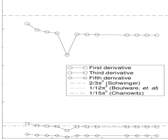
Figure 2: Coefficients of three spectral fit for different lattice sizes. ($\mu=0$) For the first derivative term, the coefficient shown is $S\Delta^{2}$.

Acknowledgements This work was supported in part by the U.S. Department of Energy and the U.S. Department of Education.

References

• [1] C. M. Bender, L. R. Mead, and K. A. Milton, “Discrete Time Quantum Mechanics,” preprint OKHEP-93-07, to be published in J. Computational and Applied Math.
• [2] J. Schwinger, Phys. Rev. Lett. 3 (1959) 296.
• [3] J. D. Bjorken, Phys. Rev. 148 (1966) 1467; K. Johnson and F. E. Low, Prog. Theor. Phys. Suppl. 37–38 (1966) 74; D. G. Boulware and R. Jackiw, Phys. Rev. 186 (1969) 1442.