Abstract

In this work the Feynman-Schwinger representation for the two-body Greens function is studied. After having given a brief introduction to the formalism, we report on the first calculations based on this formalism. In order to demonstrate the validity of the method, we consider the static case where the mass of one of the particles becomes very large. We show that the heavy particle follows a classical trajectory and we find a good agreement with the Klein-Gordon result.

1 Theory

Recently, the Feynman-Schwinger representation (FSR) was presented [1] as a new covariant formalism to calculate the relativistic two-body Greens function. It was shown that the FSR sums up all ladder and crossed diagrams and that it has the correct static limit if one of the masses of the two particles becomes very large. Furthermore it was argued that the formulation was well suited for essentially nonperturbative gauge theories such as QCD, since the formalism can be set up in a gauge invariant way and the possibility exists to include a vacuum condensate in the interaction kernel via the cumulant expansion. While the formalism neglects all valence particle loops, one has the possibility to include all self-energy and vertex-correction graphs as well. In this paper however, we will concentrate on the static limit.

In order to demonstrate the formalism we consider the $\phi^{3}$-theory for two charged particles $\chi_{1}$ and $\chi_{2}$ with masses $m_{1}$ and $m_{2}$ and charges $g_{1}$ and $g_{2}$, interacting through exchange of a third, neutral particle $\phi$ with mass $\mu$. The Euclidean action for this theory is:

$$S_{E} = \int{\rm d}^{4}x\left[\chi_{i}^{\dagger}\left(m_{i}^{2}-\partial_{\mu}^{2}+g_{i}\phi\right)\chi_{i}+\mbox{$\frac{1}{2}$}\phi\left(\mu^{2}-\partial_{\mu}^{2}\right)\phi\right]$$

$$\equiv \int{\rm d}^{4}x\left[\chi_{i}^{\dagger}\Lambda_{i}\chi_{i}+\mbox{$\frac{1}{2}$}\phi\left(\mu^{2}-\partial_{\mu}^{2}\right)\phi\right]$$

where summation over the index $i$ is implied. The Greens function is defined as the transition probability from the initial state $\Psi_{\rm i}=\chi^{\dagger}_{1}(x_{1})\chi_{2}(x_{2})$ to the final state $\Psi_{\rm f}=\chi_{1}(y_{1})\chi_{2}^{\dagger}(y_{2})$:

$$G(y_{1},y_{2}|x_{1},x_{2})\propto\int{\cal D}\chi_{1}{\cal D}\chi_{2}{\cal D}\phi\;\;\Psi_{\rm f}\Psi_{\rm i}\;\;{\rm e}^{-S_{E}}$$

$$\propto\int{\cal D}\phi\;\left(\det\Lambda_{1}(y_{1},x_{1})\Lambda_{2}(y_{2},x_{2})\right)^{-\frac{1}{2}}\;\Lambda_{1}^{-1}(y_{1},x_{1})\Lambda_{2}^{-1}(y_{2},x_{2})\;\;{\rm e}^{-\frac{1}{2}\int{\rm d}^{4}x\;\phi\left(\mu^{2}-\partial_{\mu}^{2}\right)\phi}$$ (2)

Next, in order to get the sum of all generalized ladder graphs, we neglect the determinant in (2). This corresponds to neglecting all the $\chi_{1}$- and $\chi_{2}$-loops and is often called the ‘quenched approximation’. We now wish to rewrite (2) in such a way that we can perform the integration over the remaining field $\phi$ as well. To this end we exploit the Feynman-Schwinger representation for $\Lambda^{-1}$:

$$\Lambda^{-1}(y,x)\;\;=\;\;\int_{0}^{\infty}{\rm d}s\left\langle y\left|{\rm e}^{-s(m^{2}-\partial_{\mu}^{2}+g\phi)}\right|x\right\rangle$$ (3)

$$= \left.\int_{0}^{\infty}{\rm d}s\lim_{N\rightarrow\infty}\left(\frac{N}{2\pi s}\right)^{2N}\int\prod_{n=1}^{N-1}{\rm d}^{4}z_{n}\;{\rm e}^{-m^{2}s-\frac{N}{4s}\sum_{i=1}^{N}\left(z_{i}-z_{i-1}\right)^{2}-\frac{gs}{N}\sum_{i=1}^{N}\phi\left(\frac{1}{2}(z_{i}+z_{i-1})\right)}\right|_{z_{0}=x}^{z_{N}=y}$$

$$= \int_{0}^{\infty}{\rm d}s\int\left({\cal D}z\right)_{xy}{\rm e}^{-m^{2}s-\frac{1}{4s}\int_{0}^{1}\dot{z}_{\mu}^{2}(\tau){\rm d}\tau-gs\int_{0}^{1}\phi(z(\tau)){\rm d}\tau}$$

Integrating over the $\phi$-field is now straightforward and yields:

$$G(y_{1},y_{2}|x_{1},x_{2})\;\;\propto$$

$$\int_{0}^{\infty}{\rm d}s_{1}\int_{0}^{\infty}{\rm d}s_{2}\int\left({\cal D}z_{1}\right)_{x_{1}y_{1}}\left({\cal D}z_{2}\right)_{x_{2}y_{2}}{\rm e}^{-m_{1}^{2}s_{1}-m_{2}^{2}s_{2}-\frac{1}{4s_{1}}\int_{0}^{1}\dot{z}_{1,\mu}^{2}(\tau_{1}){\rm d}\tau_{1}-\frac{1}{4s_{2}}\int_{0}^{1}\dot{z}_{2,\mu}^{2}(\tau_{2}){\rm d}\tau_{2}}\left\langle W_{\phi}\right\rangle$$ (4)

In case we leave out the self-energy contribution and the vertex-corrections, the Wilson loop $\left\langle W_{\phi}\right\rangle$ is simply given by:

$$\left\langle W_{\phi}\right\rangle = \exp\left[-\frac{g_{1}g_{2}s_{1}s_{2}}{N^{2}}\sum_{j,k=1}^{N}\Delta\left(\mbox{$\frac{1}{2}$}\left(z_{1,j}+z_{1,j-1}-z_{2,k}-z_{2,k-1}\right)\right)\right]$$ (5)

$$= \exp\left[-g_{1}g_{2}s_{1}s_{2}\int_{0}^{1}\int_{0}^{1}\Delta\left(z_{1}(\tau_{1})-z_{2}(\tau_{2})\right){\rm d}\tau_{1}{\rm d}\tau_{2}\right]$$

where $\Delta$ is the free scalar two-point function:

$$\Delta(z)=\frac{\mu}{4\pi^{2}\left|z\right|}K_{1}(\mu\left|z\right|)$$ (6)

This formulation for the Greens function has the great advantage that it is essentially a quantummechanical one in which the two valence particles interact via a nonlocal interaction. One can show that (4) and (5) sum up all ladder and crossed diagrams. Furthermore, if $m_{2}\rightarrow\infty$ then $G$ obeys the following Klein-Gordon equation:

$$\left(\partial_{\mu}^{2}-m_{1}^{2}-\frac{g_{1}g_{2}}{2m_{2}}V(\left|{\bf r}\right|)\right)G(r)=\delta^{(4)}(r)$$ (7)

with

$$V(\left|{\bf r}\right|)=\int_{-\infty}^{\infty}{\rm d}t\;\;\Delta\left(\sqrt{\left|{\bf r}\right|^{2}+t^{2}}\right)$$

which reduces to the instantaneous Coulomb interaction for the case $\mu\rightarrow 0$.

2 Results

For a Euclidean theory it is known that for large times $T=\frac{m_{1}(y_{1,4}-x_{1,4})+m_{2}(y_{2,4}-x_{2,4})}{m_{1}+m_{2}}$ the contributions to $G$ are dominated by the lowest lying states and that they fall off exponentially, $G=\sum_{i}c_{i}\exp(-E_{i}T)$. Hence, we can obtain the ground state energy by observing that:

$$E_{0}=-\lim_{T\rightarrow\infty}\frac{{\rm d}}{{\rm d}T}\log G=-\lim_{T\rightarrow\infty}\left(\frac{{\rm d}}{{\rm d}T}G\right)/G$$ (8)

The time derivative with respect to $T$ can be done explicitely.

We project the Greens function on a complete set of total and angular momentum states $\left|{\bf P},l,m\right\rangle$, but due to the nonlocal interaction (5) this does not imply that the degrees of freedom that are associated with the generators of the symmetries (${\bf P}$, $L^{2}$, $L_{z}$), can be integrated out.

For all our calculations we used the Metropolis Monte Carlo algorithm to perform the integrations over $s_{1}$, $s_{2}$ and all the coordinates. The value of $N$ in (3) and (5) that we needed to get reasonably stable results was typically 25, so that effectively we had to perform a 200-dimensional integral. Convergence was usually reached after $3\cdot 10^{8}$ points which took approximately 30 hours of CPU-time on our fastest workstation.

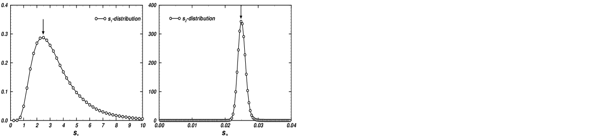
Figure 1: Normalized distributions of $s_{1}$ and $s_{2}$. The arrows indicate the classical values.

In order to demonstrate that it is indeed possible to determine the actual groundstate within this formalism, we have investigated the case of one light and one heavy particle interacting through exchange of a massless third particle ($m_{1}=1$, $m_{2}=100$ and $\mu=0$). For the strength of the coupling we took $g^{2}\equiv-g_{1}g_{2}=4500$. The distributions of the coordinates of particle 2 are confined to a very narrow region around their classical values, demonstrating that the heavy particle indeed follows a classical trajectory. Particle 1 shows much more quantum behavior; its distributions have finite widths. The normalized distributions of $s_{1}$ and $s_{2}$ are shown in figure 1. Note the difference in scales between both distributions.

In figure 2 we show the average of 5 runs as a function of the number of Monte Carlo points. The exact result for $m_{2}\rightarrow\infty$, obtained by solving the Klein-Gordon equation (7), is $E_{0}=100.55$ and is indicated by the arrow on the right hand side of the figure. The FSR-result fluctuates around this value and the average over the last $4\cdot 10^{8}$ Monte Carlo points is $E_{0}=100.57\pm 0.02$. This clearly demonstrates the feasibility of the method.

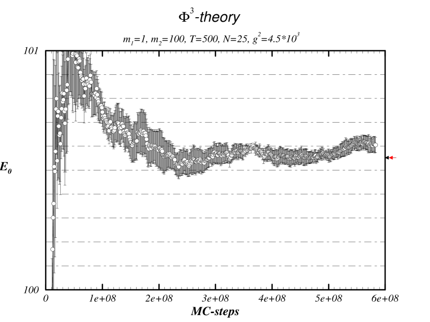
Figure 2: Bound-state mass in the static limit as a function of the number of Monte Carlo points. $T$ is given in units of the inverse total mass.

We have also studied in detail the situation where $m_{1}=m_{2}=1$ and $\mu=0$. This case is well suited to test the ladder approximation since the solution of the Bethe-Salpeter equation in the ladder approximation is known exactly [2, 3, 4]. For values of the coupling constant such that there is a binding energy of roughly 10% of the mass of the constituents, we find that the full results lie substantially below the ladder predictions.

In conclusion, we have demonstrated that the FSR is well suited for going beyond the ladder theory in the study of composite systems in field theory. In particular, ground state properties such as the binding energies and bound-state wave functions can readily be determined with this method.

References

• [1] Yu. A. Simonov and J. A. Tjon, The Feynman-Schwinger Representation for the Relativistic Two-Particle Amplitude in Field Theory, Ann. Phys., to be published.
• [2] N. Nakanishi, Behavior of the Solutions to the Bethe-Salpeter Equation, Prog. Theor. Phys. Suppl. 95 (1988) 1-117 and references therein.
• [3] G. C. Wick, Properties of Bethe-Salpeter Wave Functions, Phys. Rev. 96 (1954) 1124-1134.
• [4] R. E. Cutkosky, Solutions of a Bethe-Salpeter Equation, Phys. Rev. 96 (1954) 1135-1141.